Dive into the Power of Neuronal Heterogeneity

Abstract

The biological neural network is a vast and diverse structure with high neural heterogeneity. Conventional Artificial Neural Networks (ANNs) primarily focus on modifying the weights of connections through training while modeling neurons as highly homogenized entities and lacking exploration of neural heterogeneity. Only a few studies have addressed neural heterogeneity by optimizing neuronal properties and connection weights to ensure network performance. However, this strategy impact the specific contribution of neuronal heterogeneity. In this paper, we first demonstrate the challenges faced by backpropagation-based methods in optimizing Spiking Neural Networks (SNNs) and achieve more robust optimization of heterogeneous neurons in random networks using an Evolutionary Strategy (ES). Experiments on tasks such as working memory, continuous control, and image recognition show that neuronal heterogeneity can improve performance, particularly in long sequence tasks. Moreover, we find that membrane time constants play a crucial role in neural heterogeneity, and their distribution is similar to that observed in biological experiments. Therefore, we believe that the neglected neuronal heterogeneity plays an essential role, providing new approaches for exploring neural heterogeneity in biology and new ways for designing more biologically plausible neural networks.

1 Introduction

The biological neural network is an intricate system, and its high heterogeneity plays a vital role in learning and reasoning. In a biological neural network, the diversity of neurons endows the network with richer functionality and computational power. Different types of neurons can respond to different types of input features, thereby providing the network with better feature extraction capabilities [1; 2; 3]. The diversity of neurons enables the biological neural network to produce meaningful responses to external stimuli even without weight training. Furthermore, the heterogeneity of neurons is closely related to the plasticity of the brain and contributes to the robustness of neural networks [4; 5].

However, conventional Artificial Neural Networks (ANNs) mainly rely on homogeneous activation functions to simulate how neurons receive information and adapt to different tasks through training the connection weights. In this process, neurons are often simplified and homogenized. In contrast, spiking neurons offer higher flexibility, and researchers can achieve different spiking patterns by adjusting various parameters [6; 7]. Nevertheless, these studies still cannot completely separate the influence of connection weights and independently optimize heterogeneous neurons. This could potentially obscure the specific contribution of neuronal heterogeneity to network performance. To address this challenge, we discuss the computational capabilities exhibited by neuronal heterogeneity when using a network without modifying the connections. Such research helps us better understand how neuronal heterogeneity independently influences and provides valuable insights for future network designs.

The success of deep learning in the field is largely attributed to the backpropagation (BP) [8]. However, there is still debate regarding whether the brain performs precise derivative computations [9]. We first uncover the challenges faced by BP in optimizing Spiking Neural Networks (SNNs), particularly in terms of stability. Additionally, we discover that the Evolutionary Strategy (ES) without BP outperforms in optimizing the parameters of random networks, which aligns more closely with biological plausibility. Through experiments involving tasks like continuous control, working memory, and image recognition, we find that optimizing neuron properties not only allows neurons to exhibit diverse spiking patterns but also achieves performance that is comparable to, or even exceeds, that obtained by optimizing connection weights (as depicted in Fig.1).

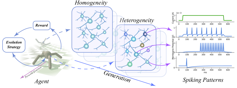
Figure 1: Diagram of Heterogeneous Neural Networks. Left: Heterogeneous SNNs with random weights can be applied to the continuous control tasks. Right: When the input current is constant, heterogeneous neurons can exhibit various spiking patterns.

Furthermore, our findings highlight the critical role of membrane time constants in neural heterogeneity. Interestingly, we observe that the distribution of these time constants in our model resembles that found in biological experiments. This suggests the significance of incorporating neglected neuronal heterogeneity in the design of biologically plausible SNNs and provides new opportunities for exploring neural heterogeneity in biology.

In particular, our contributions to the exploration of the role of neuronal heterogeneity are as follows:

• We highlight the challenges of BP in optimizing SNNs, particularly in long sequence tasks, and show that BP-free evolutionary algorithms can yield better results.

• We employ ES to optimize the properties of neurons in a network with random weights. Experimental results demonstrate that the random weight networks with heterogeneous neurons can achieve comparable or even higher performance than the network with homogeneous neurons and trainable weights.

• Our ablation analysis underscores the importance of membrane time constants in neural heterogeneity and their distribution similarities with biological experiments.

2 Related Works

2.1 Neural heterogeneity

Recent studies highlight the critical role of heterogeneous neurons in enhancing the robustness and performance of SNNs [10; 11]. This heterogeneity extends to neuron connectivity, synaptic properties, learning rules, and characteristics. For instance, the use of Hebbian learning rules for dynamic weight optimization allows networks to better adapt to unforeseen damages, enhancing their resilience and performance [12]. Similarly, dynamic neuron heterogeneity can distinguish temporal patterns [13], while the Heterogeneous Recurrent SNN (HRSNN) outperforms homogeneous SNNs in video activity recognition and classification [14].

Neuronal properties, such as membrane time constants, greatly influence brain dynamics and functions [15; 16; 17]. Despite this, few studies have modeled neuron heterogeneity in SNNs. Such modeling can enhance SNNs’ performance in real-time tasks [18] and accelerate learning [6]. However, optimization of both synaptic weights and neuronal properties is challenging and makes it hard to determine the specific impact of neuronal heterogeneity. Previous research has concentrated on analyzing membrane time constants, often overlooking other spiking neurons properties like threshold voltage and resting potential. In response to these gaps in the existing literature, our work focuses on investigating the importance of heterogeneous neurons in a network with random weights, and the distinct contributions of different neuronal properties.

2.2 Randomized Networks

Weight Agnostic Neural Networks (WANNs), first introduced by Gaier and Ha [19], deviate from conventional deep learning by prioritizing architecture over weight fine-tuning. This approach allows WANNs to perform tasks effectively with random or shared weights, resulting in efficient and lightweight models. Network training is achieved by adjusting the architecture and neuron activation functions, employing a minimalistic algorithm, NeuroEvolution of Augmenting Topologies (NEAT) [20], for evolving network architectures.

Despite using suboptimal weights, WANNs perform competitively on tasks like CartPole, bipedal locomotion, and MNIST [21]. However, their use of continuous non-linear activation functions and limited weight evaluation per structure can increase training costs, posing a challenge for efficient learning.

Following the pioneering work of Gaier and Ha [19], we examine the role of neuron heterogeneity in fixed, randomly initialized SNNs without the influence of other optimizable parameters.

3 Method

3.1 Heterogeneous Spiking Neuron

The Leaky Integrate-and-Fire (LIF) neuron is a simplified neuron model used to study the dynamic behavior of neural networks. It is an abstraction from the behavior of biological neurons, describing neurons’ charging and discharging process through a relatively simple mathematical model. The LIF neuron model is widely used in computational neuroscience because it strikes a good balance between capturing the essential dynamic characteristics of neurons and computational complexity. The basic formula of the LIF neuron model can be expressed as follows:

$$\tau_{m}\frac{\partial v}{\partial t}=-(v-v_{rest})+RI(t)$$ (1)

In Eq. 1, $\tau_{m}$ is the membrane time constant, determining the speed of the neuron’s charging and discharging processes. $I(t)$ represents the input current, and $v_{rest}$ is the resting potential, which determines the neuron’s membrane potential when there is no input current. $R$ is the membrane resistance, and $v_{th}$ is the threshold potential. When the membrane potential reaches $v_{th}$, the neuron fires a spike, and the membrane potential returns to the resting potential. It is often necessary to discretize the LIF neuron model to perform numerical simulations. The neuron dynamics equation can be discretized using the Euler method:

$$u(t) =v(t-\Delta t)+\frac{\Delta t}{\tau_{m}}(R\sum_{i}w_{i}s_{i}(t)-v(t-\Delta t)+v_{rest})$$ (2)

$$s(t) =g(u(t)-v_{th})$$

$$v(t) =u(t)(1-s(t))+v_{reset}s(t)$$

In Eq. LABEL:lif, $\Delta t$ is the time step, $v_{reset}$ is the reset potential, $u(t)$ and $v(t)$ represent pre- and post-spike membrane potentials, and $g(\cdot)$ is the Heaviside function modeling spiking behavior. Synaptic weights, represented as $w_{i}$, are often prioritized in conventional neural networks. Despite this, our study focuses on the overlooked aspect of neuronal heterogeneity in randomly weighted SNNs, aiming to optimize neuron parameters like membrane time constant, membrane resistance, resting potential, and threshold voltage. In the experimental section, we make $v_{reset}=v_{rest}$ for simplicity.

3.2 Spiking Neurons: Iterative Dynamical System

In control theory and reinforcement learning, the primary objective is to optimize a control variable towards a specific objective function along a trajectory. For instance, we aim to find a policy that minimizes the expected total cost or maximizes the expected total reward within a finite time horizon. To evaluate the quality of a policy, it is common to define a loss function that measures the performance of the policy over a finite number of steps $N$. For example, when considering the output of a neural network as the membrane potential of its last layer, we can define the following loss function, which sums up the losses $L_{n}$ computed up to a finite step $N$.

$$L(\theta)=\frac{1}{N}\sum_{n=0}^{N-1}l_{n}(v(n\Delta t);\theta)$$ (3)

In Eq. 3, $\theta$ denotes the set of trainable parameters. In this context, the trainable parameters are the neuron parameters, i.e., $\theta=\{\tau_{m},v_{th},v_{rest},R\}$. For gradient-based optimization methods, the derivative of the loss function is of particular interest. The derivative of the loss function at time $t$ can be expressed as:

$$\frac{\partial L_{n}}{\partial\theta} =\frac{\partial l_{t}}{\partial v(t)}\frac{\partial v(t)}{\partial\theta}+\frac{\partial l_{t}}{\partial v(t)}\frac{\partial v(t)}{\partial v(t-\Delta t)}\frac{\partial v(t-\Delta t)}{\partial\theta}+\dots+\frac{\partial l_{t}}{\partial v(t)}\dots\frac{\partial v(\Delta t)}{\partial v(0)}\frac{\partial v(0)}{\partial\theta}$$ (4)

$$=\sum_{k=0}^{n}\frac{\partial l_{n}}{\partial v(t)}(\prod_{i=k+1}^{n}\frac{\partial v(i\Delta t)}{\partial v((i-1)\Delta t)})\frac{\partial v(k\Delta t)}{\partial\theta}$$

According to Eq. 3, the total gradient of $L(\theta)$ with respect to $\theta$ is:

$$\nabla_{\theta}L(\theta)=\frac{1}{N}\sum_{n=0}^{N}[\sum_{k=0}^{n}\frac{\partial l_{n}}{\partial v(t)}(\prod_{i=k+1}^{n}\frac{\partial v(i\Delta t)}{\partial v((i-1)\Delta t)})\frac{\partial v(k\Delta t)}{\partial\theta}]$$ (5)

Eq. 5 involves a cumulative product of the Jacobian matrix, which corresponds to the membrane potential transfer function of the LIF neuron. According to Eq. LABEL:lif, its recursive form can be derived.

$$\frac{\partial v(t)}{\partial v(t-\Delta t)}=[1-s(t)+(v_{rest}-u(t))g^{\prime}(u(t)-v_{th})](1-\frac{\Delta t}{\tau_{m}})$$ (6)

In Eq. 6, $g^{\prime}$ represents the derivative of the Heaviside function. Due to its non-differentiability, an approximate form is often used, known as a surrogate function [22]. The surrogate gradient provides the convenience of optimizing SNNs through backpropagation but also introduces inaccuracies in gradient estimation. When some or all of the eigenvalues in $\prod_{i=k+1}^{n}(\frac{\partial v(i\Delta t)}{\partial v((i-1)\Delta t)})$ of Eq. 5 are larger than $1$, the system may diverge [23]. Additionally, $u(t)$ represents the membrane potential before the spike, which is generally considered unbounded and can have large absolute values in practice [24]. This makes it challenging to ensure the stability of the dynamical system, especially for long sequence tasks, when using backpropagation to optimize SNNs. To mitigate this issue, some studies disconnect the gradient flow for $v(t)$ and $s(t)$ in applications [25] to ensure that the magnitude of Eq. 6 is smaller than $1$, thereby ensuring system stability. However, this approach also results in exponentially decaying gradients along the time dimension, limiting the long-term memory capacity of SNNs.

3.3 Evolutionary Strategy

A viable approach discards gradients and uses black-box methods to estimate the optimization direction, alleviating the storage cost issue of storing all trajectories in BP Through Time (BPTT) [26]. We explore neuronal heterogeneity using BP-free evolutionary methods, contrasting with gradient-based methods.

Specifically, we estimate the gradient more robustly by adding perturbations. Assuming the standard deviation of the perturbation is $\sigma$, the initial neuron parameters are $\theta_{0}$, and $M$ perturbations $\epsilon_{i}\sim\mathcal{N}(0,I)$ are sampled from a standard normal distribution. Then, the estimate of the gradient of the loss with respect to the perturbation is:

$$\nabla_{\theta}L_{ES}(\theta)=\mathbb{E}_{\epsilon\sim\mathcal{N}(0,I)}\{\frac{\epsilon}{\sigma}L(\theta+\sigma\epsilon)\}=\mathbb{E}_{\epsilon\sim\mathcal{N}(0,I)}\{\frac{\epsilon}{\sigma}(L(\theta+\sigma\epsilon)-L(\theta))\}$$ (7)

According to Eq. 7, the update of the neuron parameters can be expressed as follows, given a learning rate of $\alpha$:

$$\theta_{t+1}\leftarrow\theta_{t}+\frac{\alpha}{\sigma M}\sum_{j=0}^{M}L(\theta_{t}+\sigma\epsilon_{j})$$ (8)

Like natural selection in biological systems, ES uses random search strategies to optimize neural network parameters. These strategies can reduce estimation errors, especially in continuous control contexts [27], compared to BPTT.

4 Result

In this section, we first compare the impact of optimizing connection weights in homogeneous neural networks and optimizing neuron properties in heterogeneous neural networks on working memory and continuous control tasks while keeping the same number of trainable parameters. We then conduct ablation analysis on different properties of neurons and compare the distribution of membrane time constants in biological neurons and SNNs. Afterward, we test heterogeneous SNNs with random weights on image classification tasks to demonstrate the generality of heterogeneous neurons. Lastly, we compare the performance of BP and ES in optimizing connection weights and neuron heterogeneity in some classic control tasks of the Gymnax environment [28]. Details regarding the network architecture, neuron parameters, hyperparameter settings, and training methods can be found in Tab. 4.

4.1 Neuronal Heterogeneity on Memory Tasks

Working memory constitutes a pivotal component of a cognitive system, allowing us to hold and manipulate task-relevant information in the short term. Neuronal heterogeneity potentially serves as a critical neural foundation for memory. Therefore, we validate this hypothesis in the memory length task within bsuite [29]. This environment is a stylized T-maze [30], consisting of $N$ steps per episode. Each state can be represented as $s_{t}=(c_{t},\frac{t}{N})$, for all $t=0,\dots,N-1$. The action space is $\mathcal{A}=\{-1,+1\}$, where $c_{0}\sim Unif(A)$ and $c_{t}=0$ for all $t\geq 1$. The reward for the memory task is $r_{N-1}=Sign(a_{N-1}=c_{0})$. The task requires the agent to remember and reproduce the initial stimulus in the final step. We conduct experiments on randomly-weighted SNNs with heterogeneous neurons and weight-trainable SNNs for diverse experimental settings, using different random seeds and repeating the experiments $50$ times of varying lengths.

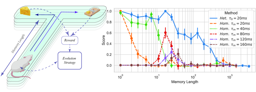
Figure 2: Left: Illustration of the memory length environment. Right: Performance of SNNs when optimizing only neuron properties and only connection weights at different memory steps.

As shown in Fig 2, SNNs with heterogeneous neurons achieve significantly better memory performance than conventional SNNs, even in the case of non-optimizable synaptic weights. With increased task difficulty, the heterogeneous SNNs can maintain a reward of about $0.9$ at $25$ steps. In contrast, the performance of homogeneous SNNs sharply decreases as the memory length increases, even with adjustments to the connection weights. To ensure the robustness of our conclusions, we conducted a hyperparameter search for the membrane time constant of homogeneous SNNs, as depicted in the right of Fig 2. For homogeneous SNNs, different membrane time constants can only achieve limited memory lengths, whereas heterogeneous SNNs demonstrate greater robustness and superior generalization, adapting well to both long-term and short-term memory tasks. It is worth noting that in this experiment, we only use feedforward SNNs, which means we rely solely on the time characteristics of neurons rather than recurrent structures to achieve working memory. This effectively demonstrates the critical role of neuron heterogeneity in memory.

4.2 Neuronal Heterogeneity on Continuous Control Tasks

We evaluate the performance of heterogeneous random-weight SNNs on a benchmark of continuous robot control problems in Google Brax library [31] and compare them with homogeneous SNNs with trainable connection weights. For all simulated environments, we reported the mean and standard deviation of the accumulated rewards across $5$ individual experiments with different random seeds.

Ant (Ant), HalfCheetah (Hc), Hopper (Hp), and Walker2d (Wal) are reinforcement learning environments in the Brax, mainly used for research and experimentation in robot motion control. The primary objective of these environments is to enable robots to move forward as swiftly as possible while maintaining a stable standing position in specific scenarios. For detailed descriptions of these environments, please refer to Section 6.3.

As shown in Fig. 3, SNNs with neuronal heterogeneity exhibit comparable or even better performance than conventional SNNs used as a baseline, with the same number of trainable parameters. As the number of trainable parameters increases, we observe that the performance of the random network with neuronal heterogeneity also improves. In contrast, the relationship between the performance of conventional SNNs and the number of trainable parameters is insignificant. This indicates that random networks with neuronal heterogeneity can better utilize the diversity of neurons, capture the relationships in the data, and improve the network’s generalization performance. In contrast, the neuronal structure of conventional SNNs is relatively simple and may not fully utilize the increased number of trainable parameters.

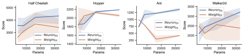
Figure 3: Comparison of rewards obtained from training neurons’ properties and connection weights on continuous control tasks.

4.3 Ablation Study of Neuronal Properties

We conduct ablation studies on heterogeneous neural networks to investigate the impact of four key properties on network performance, including membrane time constant, resting potential, threshold voltage, and membrane resistance. The experiments involve removing one or more of these four properties and evaluating their importance by observing changes in network performance. In all SNNs, the number of trainable parameters is set to $16,384$.

Table 1: Ablation study of neuronal properties. $\checkmark$ indicates that the neuron property is trainable, while others indicate that the neuron property is fixed to its default initial value.

Neuronal Properties				Reward (mean/stdev)
$\tau_{m}$	$v_{th}$	$v_{rest}$	$R$	Hc	Ant	Hp	Wal
✓	-	-	-	$3967\pm 171$	$1180\pm 200$	$1796\pm 9$	$2580\pm 351$
-	✓	-	-	$101\pm 24$	$431\pm 18$	$399\pm 12$	$750\pm 254$
-	-	✓	-	$3544\pm 236$	$680\pm 19$	$1502\pm 9$	$2286\pm 549$
-	-	-	✓	$3264\pm 528$	$732\pm 60$	$1654\pm 29$	$2143\pm 551$
✓	✓	-	-	$3110\pm 749$	$1046\pm 11$	$1982\pm 154$	$2866\pm 402$
✓	-	✓	-	$3887\pm 637$	$1160\pm 215$	$2016\pm 94$	$2184\pm 669$
✓	-		✓	$3460\pm 331$	$953\pm 50$	$2031\pm 13$	$3140\pm 216$
-	✓	✓	-	$3335\pm 248$	$765\pm 172$	$448\pm 89$	$2880\pm 174$
-	✓	-	✓	$2679\pm 406$	$838\pm 14$	$1771\pm 12$	$2674\pm 99$
-	-	✓	✓	$3587\pm 193$	$457\pm 413$	$1902\pm 9$	$2286\pm 549$
✓	✓	✓	-	$3924\pm 342$	$967\pm 57$	$1914\pm 21$	$2431\pm 19$
✓	✓	-	✓	$3724\pm 472$	$1119\pm 85$	$1828\pm 15$	$2880\pm 174$
✓	-	✓	✓	$3982\pm 319$	$1276\pm 18$	$1943\pm 34$	$2779\pm 73$
-	✓	✓	✓	$3214\pm 204$	$978\pm 21$	$1790\pm 26$	$2529\pm 38$
✓	✓	✓	✓	$4221\pm 413$	$1221\pm 35$	$2142\pm 27$	$2699\pm 404$

As shown in Tab. 1, the results show that the membrane time constant significantly impacts the network performance, while other properties’ influence is relatively minor. To further quantitatively analyze the correlations between different neuron attributes and their impact on model performance, we utilized Shapley Value analysis to assess the average expected boundary contributions of various attributes, as shown in Fig. 4. This suggests that the membrane time constant is crucial when designing networks with heterogeneous neurons and requires special attention for optimizing network performance.

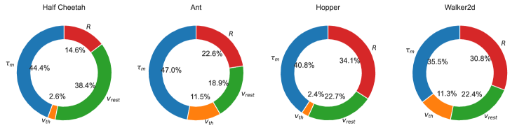
Figure 4: Analysis of different properties of heterogeneous neurons by Shapley values.

4.4 Comparison of Membrane Time Constants Distributions and Experimental Data

In this subsection, we compare our model’s membrane time constant distributions with some experimental biological data to verify whether our heterogeneous neurons are consistent with biological phenomena. We visualize the membrane time constant distribution learned from models with homogeneous initial values and compare it with that observed in layer $4$ spiny cells in mouse primary visual cortex [32] and spiny cells in the temporal lobe gyrus of humans [33], as shown in Fig. 5.

Although our model is only designed for a single task, the distribution of membrane time constants of the neurons in the model exhibits a substantial similarity to some biological evidence, which shows a long-tail distribution. For the memory length task, we find that for short delays, the membrane potential distribution is more concentrated, while for longer memory tasks, the membrane time constant increases to adapt to longer delays. To quantify this similarity, we fit the data using both lognormal distribution and gamma distribution, and the results are shown in Fig. 5 and Tab. 2.

The similarity with biological neurons suggests that the constructed model can simulate some characteristics of the biological nervous system to a certain extent. This similarity may provide neuroscientists with a better understanding of the distribution of membrane time constants of neurons and also indicates that heterogeneous neurons may have a higher effectiveness in simulating the behavior of biological neurons. This also provides confidence for further research using this model.

Table 2: Fitting results of membrane time constants for reinforcement learning tasks and biological experiments. The location parameter is set to $0$.

Distributions		Hc	Ant	Hp	Wal	Mouse V1	Human MTG
gamma	shape	$1.46$	$1.85$	$2.20$	$1.85$	$1.64$	$3.18$
	scale	$14.6$	$11.7$	$10.0$	$11.8$	$13.4$	$9.11$
log normal	shape	$0.26$	$0.28$	$0.30$	$0.28$	$0.27$	$0.33$
	scale	$20.6$	$20.7$	$20.9$	$20.8$	$21.1$	$27.3$

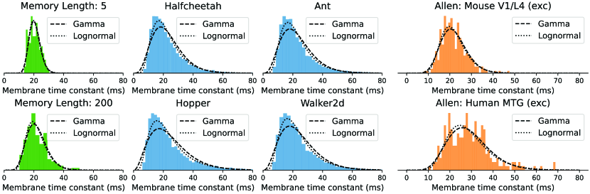
Figure 5: Left: Distribution of membrane time constants in reinforcement learning tasks. Right: Distribution of membrane time constants in biological experiments.

4.5 Heterogeneous Spiking Neural Networks on Classification Tasks

Although the model is designed for a single reinforcement learning task, the similarity between its membrane time constant distribution and experimental biological data suggests that the model may have some universality and can be applied to other similar tasks.

The results of the reinforcement learning task validate the crucial role of neural heterogeneity, even when the model cannot learn new knowledge through updating synaptic weights. We further test our model on higher-dimensional image classification tasks to verify the potential of heterogeneous SNNs in other tasks. Specifically, we test our model on two commonly used image datasets: MNIST [21] and FashionMNIST [34]. MNIST consists of 10-digit classes, while FashionMNIST contains $10$ different types of clothing. Since static image data requires a shorter simulation time, the total simulation time for both datasets was set to $4$ simulation steps.

Table 3: Comparison of heterogeneous SNNs and conventional SNNs on image classification tasks.

Parameter	MNIST		FashionMNIST
Neuron / Weight	Neuron	Weight	Neuron	Weight
4096 / 3970	$\bf 80.96\%$	$78.66\%$	$\bf 76.35\%$	$48.33\%$
8192 / 7940	$85.64\%$	$\bf 88.69\%$	$\bf 77.64\%$	$58.15\%$
16384 / 16674	$88.89\%$	$\bf 90.59\%$	$79.31\%$	$\bf 80.41\%$
32768 / 33348	$90.84\%$	$\bf 91.29\%$	$80.90\%$	$\bf 81.22\%$

Tab .3 shows the test accuracy of heterogeneous and homogeneous SNNs on the image classification task. When the number of parameters is low, heterogeneous SNNs may utilize their internal diversity to capture input data features better. Compared to homogeneous SNNs, the neurons in heterogeneous SNNs have different characteristics, which can help the network learn more diverse representations. As the number of parameters increases, homogeneous SNNs may gradually overcome the limitations caused by their simple structure. Increasing the number of parameters may give the network more expressive power, thereby partially compensating for the shortcomings of homogeneous SNNs in processing complex data. Herefore, in cases with low parameters, heterogeneous SNNs are more suitable for handling complex tasks because they can use diversity to capture the features of the data.

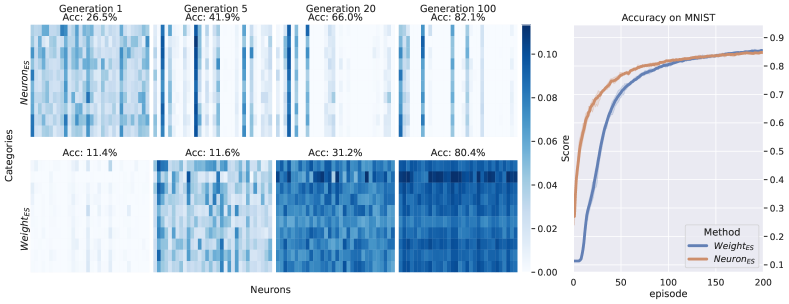
Figure 6: Spike frequency of randomly selected $32$ neurons in different generations for different categories on the MNIST dataset.

In addition to the conclusions related to accuracy, we have uncovered an intriguing phenomenon: notable distinctions in the activity patterns of neurons in heterogeneous networks compared to homogeneous SNNs. As depicted in Fig. 6, we randomly select a subset of neurons and visualize their average spiking rates for different input stimuli representing different categories. It is observed that during the initial stages of training, nearly all neurons in the heterogeneous SNNs exhibit spiking activity, resulting in faster convergence of the model. As training progressed, only a minority of neurons maintain high firing rates, while most remain silent. These active neurons can efficiently respond to stimuli from different categories through their special firing rates. In contrast, homogeneous SNNs exhibit an increasing trend in neuron firing rates during weight optimization. Although homogeneous models eventually achieve high performance, it comes at the cost of higher average firing rates of neurons.

4.6 Discussion on Backpropagation and Evolutionary Strategies

As discussed in Section 3.2, BP may lead to divergent results when applied to dynamic systems of unstable nature. In the case of LIF neurons, which are non-differentiable, surrogate gradient functions need to be introduced to establish an approximate BP pathway. However, this estimation may cause inaccurate gradient estimates. As the length of the task sequence increases, the resulting variance of the gradient estimation can lead to a more unstable system. Therefore, we use gradient-free ES for optimizing heterogeneous SNNs. Although we lose a dimension of the efficiency factor, we can obtain more stable estimates of the optimization direction. To verify the above theory, we compared the performance of gradient-based optimization methods [35] and black-box optimization methods on homogeneous and heterogeneous SNNs in some classical control tasks.

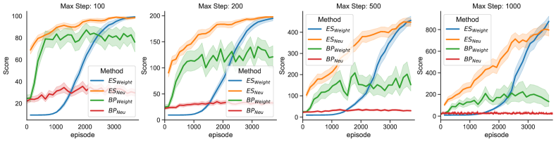
Figure 7: Performance of different optimization methods on homogeneous/heterogeneous SNNs on CartPole-v1 environment.

As shown in Fig 7, we study the effect of different sequence lengths on the model’s performance in the CartPole-v1 task. We tested the model’s performance with a maximum number of steps set to $100$, $200$, $500$, and $1000$, and repeated each experiment $100$ times with different random seeds. For ES, the population size is set to 128, and the number of iterations was set to $30$, which means a total of $3,840$ episodes of interaction with the environment. The y-axis represents the cumulative reward of the agent, which means the number of steps where the pole angle is less than $12^{\circ}$.

For homogeneous SNNs, the BP-based method converges faster than ES. However, as the sequence length increases, BP-based SNNs struggle to converge to the optimal value, while ES can robustly converge higher rewards. Furthermore, BP-based methods cannot handle untrainable weights, whereas ES can efficiently interact with the environment and achieve better results than BP-based methods in fewer episodes. This suggests that ES can better exploit the diversity of neural elements when searching the solution space and thus find better solutions in some cases. Additionally, ES evaluates and optimizes policies by directly interacting with the environment, which may be closer to the learning process in biological neural systems.

5 Discussion

In this study, we investigate the role of neuronal heterogeneity in SNNs, with a particular focus on optimizing neuronal properties without modifying the connection weights. Our research reveals the challenges faced by BP-based methods in optimizing spiking neurons, especially in dealing with long sequence tasks. As an alternative approach, we find that evolutionary strategies perform better in optimizing neuronal parameters in random networks. Through experiments on tasks such as working memory, continuous control, and image recognition, we demonstrate that optimizing neuronal properties can achieve comparable or even superior performance compared to optimizing connection weights. This highlights the importance of neuronal heterogeneity in network performance, particularly in tasks with rich temporal structures. We emphasize the role of membrane time constants in neuronal heterogeneity, and our model distribution reflects observations from biological experiments. This work contributes to the understanding of neuronal heterogeneity in both biological and SNNs, providing insights for future research in biologically-inspired neural networks.

While our study contributes to understanding neuronal heterogeneity in biological and SNNs, there are limitations that should be acknowledged. We used simplified models of spiking neurons, and real biological neurons exhibit more complex behaviors influenced by various physiological factors, all of which contribute to neuronal heterogeneity. Therefore, the behavior of our model may not fully capture the behavior of biological neurons.

In our future work, we plan to address these limitations by studying more complex neuronal models, integrating more biological observations, exploring novel optimization methods, and testing in broader tasks and domains. By delving deeper into these areas, we aim to advance our understanding of neural networks and enhance their capabilities.

6 Network Settings and Training Details

6.1 Spiking Neurons: System Stability Analysis

The spiking neuron can be regarded as an iterative dynamic system. When using gradient optimization for optimization, as mentioned in the text, the gradient of the reset membrane potential over time can be represented as follows:

$$\frac{\partial v(t)}{\partial v(t-\Delta t)}=[1-s(t)+(v_{rest}-u(t))g^{\prime}(u(t)-v_{th})](1-\frac{\Delta t}{\tau_{m}})$$ (9)

In Eq 9, $u(t)$ represents the membrane potential before the reset, which is unbounded. We visualize the membrane time constants of neurons when training SNNs with BPTT on the CartPole-v1. The neuron parameters are the same as those in Tab. 4.

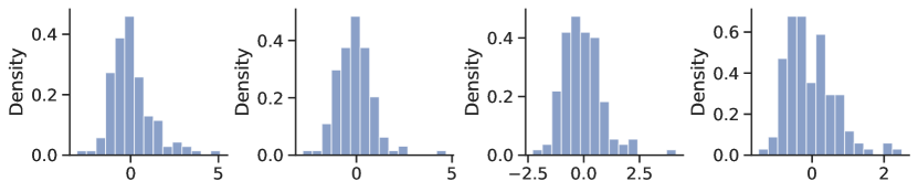
Figure 8: The distribution of membrane potentials in four different episodes of the CartPole-v1.

As shown in Fig 8, in practice, $u(t)$ is unbounded and can reach approximately $5$. This can result in the magnitude of $\frac{\partial v(t)}{\partial v(t-\Delta t)}$ being greater than $1$, leading to system divergence. Additionally, in Eq. 9, there is a term $1-s(t)$, which means that as long as $(v_{rest}-u(t))g^{\prime}(u(t)-v_{th})\geq 0$ and the neuron is not firing, there is a risk of system divergence.

Due to the non-differentiability of the Heaviside function, it is necessary to approximate the gradient of $g(\cdot)$ using a surrogate gradient [22]. One commonly used proxy gradient function can be represented as follows:

$$g^{\prime}(u(t)-v_{th})=\frac{1}{v_{th}^{2}}\max(0,v_{th}-\left|u(t)-v_{th}\right|)$$ (10)

In practical applications, there are two strategies for optimizing spiking neurons. One approach considers the impact of spikes and resets on the neuron, as shown in Eq. 9. The other approach ignores the influence of resets on gradients and can be represented as follows:

$$\frac{\partial v(t)}{\partial v(t-\Delta t)}=[1-s(t)](1-\frac{\Delta t}{\tau_{m}})$$ (11)

Eq. 11 neglects the term $\frac{\partial v(t)}{\partial s(t)}$, which ensures that $\left|\frac{\partial v(t)}{\partial v(t-\Delta t)}\right|<1$, thereby maintaining system stability. However, this leads to the exponential decay of the temporal gradients with increasing sequence length, making it challenging for the network to establish robust temporal dependencies and limiting its ability to handle tasks with strong temporal correlations. Specifically, for neuron properties, this also removes $v_{rest}$ and $v_{th}$ from the temporal gradient path, further restricting the potential of heterogeneous SNNs.

6.2 Network Structure and Hyperparameters

Table 4: Initial parameters of the spiking neurons.

Parameter	Value	Description
$\Delta t$	$5$ ms	Simulation time step
$\tau_{m}$	$20$ ms	Membrane time constant
$v_{th}$	$0.5$ V	Membrane threshold
$v_{rest}$	$0$ mV	Resting & Reset potential
$R$	$5\times 10^{7}\Omega$	Membrane Resistance

We conduct experiments using the Jax framework [36] with NVIDIA A100 40G GPU. In all experiments, the network architecture is set as a 2-layer perception, with varying trainable parameters achieved by adjusting the number of neurons in the hidden layer. The LIF model is shown in Eq. LABEL:lif, and the same method as [37] controls the neuron’s spiking. When training the connection weights, the parameters of the neurons are set as shown in Tab. 4. When optimizing heterogeneous neurons, synaptic weights were fixed, and neuron parameters, including $\tau_{m},v_{th},v_{rest},R$, are set as trainable parameters with the same initial values as when training connection weights. For $\tau_{m}$, an indirect optimization of the membrane time constant is performed using $k(\tau_{m})=\frac{1}{1+e^{-\tau_{m}}}$.

For all cases, connection weights are initialized using LeCun initialization [38]. PGPE [39] is used as the optimization algorithm, with a population size of $256$, and unless otherwise specified, trained for $1000$ generations. The average reward and standard deviation of all individuals in the last generation are reported. The center learning rate $lr_{center}$ is set to $0.15$, the learning rate for the standard deviation of the Gaussian distribution $lr_{std}$ is set to $0.1$, and the initial standard deviation $\sigma_{0}$ are set to $0.1$.

For comparison experiments using BPTT, the optimizer is Adam [40], with a learning rate $lr_{bp}=3\times 10^{-2}$. To address the non-differentiability issue of spiking neurons, the same surrogate gradient function as in [25] is used to establish the backward propagation path of the SNNs.

In the context of backpropagation, several parameters can influence the stability of the optimization process, such as the learning rate and, uniquely for SNNs, the shape and parameters of the surrogate gradient function. Therefore, to demonstrate the robustness of the conclusions in this paper, we conducted a search for hyperparameters, including learning rates and surrogate gradient-related parameters, when optimizing on the CartPole-v1 task using backpropagation.

Table 5: Hyperparametric search for learning rate $lr_{bp}$ on CartPole-v1 task.

	Max step	$1\times 10^{-3}$	$1\times 10^{-2}$	$3\times 10^{-2}$	$0.1$	$0.3$
WeightBP	100	55.7	84.3	81.2	90.2	39.9
	200	64.7	124.6	127.3	146.1	94.6
	500	52.3	161.5	183.7	201.1	34.6
	1000	52.9	114.8	190.7	228.3	40.6
NeuronBP	100	46.9	55.4	55.3	62.2	50.4
	200	55.42	63.9	62.3	63.1	57.6
	500	60.0	73.4	63.5	74.4	61.0
	1000	50.4	73.9	76.4	80.5	62.9

Table 6: Hyperparametric search for surrogate function on CartPole-v1 task.

Surrogate Function		$g(x)=\frac{1}{\pi}\arctan(\frac{\pi}{2}\alpha x)+\frac{1}{2}$				$g(x)=\mathrm{NonzeroSign}(x)\log(|\alpha x|+1)$
	Max step	$a=0.5$	$a=1$	$a=2$	$a=4$	$a=0.5$	$a=1$	$a=2$	$a=4$
WeightBP	100	87.1	87.3	81.2	85.7	79.8	84.7	85.7	81.3
	200	120.4	157.6	127.3	146.7	117.5	124.6	119.3	102.6
	500	201.3	232.6	183.7	177.7	166.7	159.3	172.8	161.3
	1000	197.6	259.1	190.7	201.4	285.2	217.5	228.7	217.6
NeuronBP	100	54.2	57.8	55.3	64.5	41.3	46.8	57.8	65.3
	200	56.4	70.8	62.3	70.1	45.0	44.2	73.0	82.8
	500	65.9	65.2	63.5	63.2	51.3	55.3	74.4	81.2
	1000	70.8	68.2	76.4	69.1	51.2	48.3	75.8	74.3

As shown in Tab. 5 and Tab. 6, the relationship between hyperparameters such as surrogate gradient functions and learning rates and performance in the CartPole task is not very pronounced. This observation further underscores the robustness of the conclusions in the manuscript. Particularly, for heterogeneous SNNs, optimizing them with backpropagation presents a challenge, and their performance is significantly inferior to evolution-based optimization strategies.

6.3 Introduction to the Continuous Control Environments

Ant (Ant), HalfCheetah (Hc), Hopper (Hp), and Walker2d (Wal) are reinforcement learning environments in the Google Brax library [31], mainly used for research and experimentation in robot motion control. The main goal of these environments is to use learning strategies to enable robots to move forward as quickly as possible and maintain stable standing positions in some environments. All environments provide feedback information about the robot’s position, velocity, angle, and joint angles for state evaluation and decision-making.

• Ant: Simulation of a quadruped robot with rewards based on movement speed and survival time.

• Hc: Simulation of a bipedal robot resembling a half-cheetah with rewards based on movement speed.

• Hp: Simulation of a monopod robot with rewards based on movement speed and survival time.

• Wal: Simulation of a bipedal walking robot with rewards based on movement speed and survival time.

References

- [1] Krishnan Padmanabhan and Nathaniel N Urban. Intrinsic biophysical diversity decorrelates neuronal firing while increasing information content. Nature neuroscience, 13(10):1276–1282, 2010.
- [2] Charles Petitpré, Haohao Wu, Anil Sharma, Anna Tokarska, Paula Fontanet, Yiqiao Wang, Françoise Helmbacher, Kevin Yackle, Gilad Silberberg, Saida Hadjab, et al. Neuronal heterogeneity and stereotyped connectivity in the auditory afferent system. Nature communications, 9(1):3691, 2018.
- [3] Johannes Lengler, Florian Jug, and Angelika Steger. Reliable neuronal systems: the importance of heterogeneity. PloS one, 8(12):e80694, 2013.
- [4] Fleur Zeldenrust, Boris Gutkin, and Sophie Denéve. Efficient and robust coding in heterogeneous recurrent networks. PLoS computational biology, 17(4):e1008673, 2021.
- [5] Alfonso Renart, Pengcheng Song, and Xiao-Jing Wang. Robust spatial working memory through homeostatic synaptic scaling in heterogeneous cortical networks. Neuron, 38(3):473–485, 2003.
- [6] Wei Fang, Zhaofei Yu, Yanqi Chen, Timothee Masquelier, Tiejun Huang, and Yonghong Tian. Incorporating Learnable Membrane Time Constant to Enhance Learning of Spiking Neural Networks. In 2021 IEEE/CVF International Conference on Computer Vision (ICCV), pages 2641–2651. IEEE, 2021.
- [7] Ahmed Shaban, Sai Sukruth Bezugam, and Manan Suri. An adaptive threshold neuron for recurrent spiking neural networks with nanodevice hardware implementation. Nature Communications, 12(1):4234, 2021.
- [8] David E. Rumelhart, Geoffrey E. Hinton, and Ronald J. Williams. Learning representations by back-propagating errors. Nature, 323(6088):533–536, 1986.
- [9] Francis Crick. The recent excitement about neural networks. Nature, 337:129–132, 1989.
- [10] Xueyuan She, Saurabh Dash, Daehyun Kim, and Saibal Mukhopadhyay. A Heterogeneous Spiking Neural Network for Unsupervised Learning of Spatiotemporal Patterns. Frontiers in Neuroscience, 14, 2021.
- [11] R. Rossi Pool and G. Mato. Spike-Timing-Dependent Plasticity and Reliability Optimization: The Role of Neuron Dynamics. Neural Computation, 23(7):1768–1789, 2011-07.
- [12] Elias Najarro and Sebastian Risi. Meta-Learning through Hebbian Plasticity in Random Networks. In Advances in Neural Information Processing Systems, volume 33, pages 20719–20731. Curran Associates, Inc., 2020.
- [13] Xueyuan She, Saurabh Dash, and Saibal Mukhopadhyay. Sequence approximation using feedforward spiking neural network for spatiotemporal learning: Theory and optimization methods. In International Conference on Learning Representations, 2021.
- [14] Biswadeep Chakraborty and Saibal Mukhopadhyay. Heterogeneous neuronal and synaptic dynamics for spike-efficient unsupervised learning: Theory and design principles. arXiv preprint arXiv:2302.11618, 2023.
- [15] Gustavo Deco, Josephine Cruzat, and Morten L. Kringelbach. Brain songs framework used for discovering the relevant timescale of the human brain. Nature Communications, 10(1):583, 2019.
- [16] Maurizio Mattia and Paolo Del Giudice. Population dynamics of interacting spiking neurons. Physical Review E, 66(5):051917, 2002.
- [17] Michael E. Hasselmo and Chantal E. Stern. Mechanisms underlying working memory for novel information. Trends in Cognitive Sciences, 10(11):487–493, 2006.
- [18] Nicolas Perez-Nieves, Vincent C. H. Leung, Pier Luigi Dragotti, and Dan F. M. Goodman. Neural heterogeneity promotes robust learning. Nature Communications, 12(1):5791, 2021-10-04.
- [19] Adam Gaier and David Ha. Weight agnostic neural networks. Advances in neural information processing systems, 32, 2019.
- [20] Kenneth O. Stanley and Risto Miikkulainen. Evolving Neural Networks through Augmenting Topologies. Evolutionary Computation, 10(2):99–127, 2002.
- [21] Yann LeCun, Corinna Cortes, and Christopher J. C. Burges. The mnist database of handwritten digits. ATT Labs [Online]. Available: http://yann. lecun. com/exdb/mnist, 2, 1998.
- [22] Sander M Bohte. Error-backpropagation in networks of fractionally predictive spiking neurons. In Artificial Neural Networks and Machine Learning–ICANN 2011: 21st International Conference on Artificial Neural Networks, Espoo, Finland, June 14-17, 2011, Proceedings, Part I 21, pages 60–68. Springer, 2011.
- [23] Erik M Bollt. Controlling chaos and the inverse frobenius–perron problem: global stabilization of arbitrary invariant measures. International Journal of Bifurcation and Chaos, 10(05):1033–1050, 2000.
- [24] Yufei Guo, Xinyi Tong, Yuanpei Chen, Liwen Zhang, Xiaode Liu, Zhe Ma, and Xuhui Huang. Recdis-snn: rectifying membrane potential distribution for directly training spiking neural networks. In Proceedings of the IEEE/CVF Conference on Computer Vision and Pattern Recognition, pages 326–335, 2022.
- [25] Yujie Wu, Lei Deng, Guoqi Li, Jun Zhu, and Luping Shi. Spatio-temporal backpropagation for training high-performance spiking neural networks. Frontiers in neuroscience, 12:331, 2018.
- [26] Zeping Yu and Gongshen Liu. Sliced recurrent neural networks. arXiv preprint arXiv:1807.02291, 2018.
- [27] Paavo Parmas, Carl Edward Rasmussen, Jan Peters, and Kenji Doya. Pipps: Flexible model-based policy search robust to the curse of chaos. In International Conference on Machine Learning, pages 4065–4074. PMLR, 2018.
- [28] Robert Tjarko Lange. gymnax: A JAX-based reinforcement learning environment library, 2022.
- [29] Ian Osband, Yotam Doron, Matteo Hessel, John Aslanides, Eren Sezener, Andre Saraiva, Katrina McKinney, Tor Lattimore, Csaba Szepesvari, Satinder Singh, et al. Behaviour suite for reinforcement learning. arXiv preprint arXiv:1908.03568, 2019.
- [30] John O’Keefe and Jonathan Dostrovsky. The hippocampus as a spatial map: preliminary evidence from unit activity in the freely-moving rat. Brain research, 1971.
- [31] C. Daniel Freeman, Erik Frey, Anton Raichuk, Sertan Girgin, Igor Mordatch, and Olivier Bachem. Brax - a differentiable physics engine for large scale rigid body simulation, 2021.
- [32] Ed S Lein, Michael J Hawrylycz, Nancy Ao, Mikael Ayres, Amy Bensinger, Amy Bernard, Andrew F Boe, Mark S Boguski, Kevin S Brockway, Emi J Byrnes, et al. Genome-wide atlas of gene expression in the adult mouse brain. Nature, 445(7124):168–176, 2007.
- [33] Michael J Hawrylycz, Ed S Lein, Angela L Guillozet-Bongaarts, Elaine H Shen, Lydia Ng, Jeremy A Miller, Louie N Van De Lagemaat, Kimberly A Smith, Amanda Ebbert, Zackery L Riley, et al. An anatomically comprehensive atlas of the adult human brain transcriptome. Nature, 489(7416):391–399, 2012.
- [34] Han Xiao, Kashif Rasul, and Roland Vollgraf. Fashion-mnist: a novel image dataset for benchmarking machine learning algorithms. arXiv preprint arXiv:1708.07747, 2017.
- [35] Ronald J Williams. Simple statistical gradient-following algorithms for connectionist reinforcement learning. Reinforcement learning, pages 5–32, 1992.
- [36] James Bradbury, Roy Frostig, Peter Hawkins, Matthew James Johnson, Chris Leary, Dougal Maclaurin, George Necula, Adam Paszke, Jake VanderPlas, Skye Wanderman-Milne, and Qiao Zhang. JAX: composable transformations of Python+NumPy programs, 2018.
- [37] Dongcheng Zhao, Yi Zeng, and Yang Li. Backeisnn: A deep spiking neural network with adaptive self-feedback and balanced excitatory–inhibitory neurons. Neural Networks, 154:68–77, 2022.
- [38] Günter Klambauer, Thomas Unterthiner, Andreas Mayr, and Sepp Hochreiter. Self-normalizing neural networks. Advances in neural information processing systems, 30, 2017.
- [39] Frank Sehnke, Christian Osendorfer, Thomas Rückstieß, Alex Graves, Jan Peters, and Jürgen Schmidhuber. Parameter-exploring policy gradients. 23(4):551–559.
- [40] Diederik P Kingma and Jimmy Ba. Adam: A method for stochastic optimization. arXiv preprint arXiv:1412.6980, 2014.