IJCAI–23 Formatting Instructions

Graph Propagation Transformer for Graph Representation Learning

Abstract

This paper presents a novel transformer architecture for graph representation learning. The core insight of our method is to fully consider the information propagation among nodes and edges in a graph when building the attention module in the transformer blocks. Specifically, we propose a new attention mechanism called Graph Propagation Attention (GPA). It explicitly passes the information among nodes and edges in three ways, i.e., node-to-node, node-to-edge, and edge-to-node, which is essential for learning graph-structured data. On this basis, we design an effective transformer architecture named Graph Propagation Transformer (GPTrans) to further help learn graph data. We verify the performance of GPTrans in a wide range of graph learning experiments on several benchmark datasets. These results show that our method outperforms many state-of-the-art transformer-based graph models with better performance. The code will be released at https://github.com/czczup/GPTrans.

1 Introduction

In many real-world scenarios, information is usually organized by graphs, and graph-structured data can be used in many research areas, including communication networks and molecular property prediction, etc. For instance, based on social graphs, lots of algorithms are proposed to classify users into meaningful social groups in the task of social network research, which can produce many useful practical applications such as user search and recommendations. Therefore, graph representation learning has become a hot topic in pattern recognition and machine learning Cai and Lam (2020); Ying et al. (2021); Brossard et al. (2020).

With the development of deep learning, many methods have been developed for graph representation learning Perozzi et al. (2014); Zhang et al. (2019); Ying et al. (2021); Hussain et al. (2021); Rampášek et al. (2022). In general, these methods can be approximately divided into two parts. The first category mainly focuses on performing Graph Neural Networks (GNNs) on graph data. These methods follow the convolutional pattern to define the convolution operation in the graph data, and design effective neighborhood aggregation schemes to learn node representations by fusing the node and graph topology information. The representative method is Graph Convolutional Network (GCN) Kipf and Welling (2016), which learns the representation of a node in the graph by considering fusing its neighbors. After that, many GCN variants Xu et al. (2018); Chen et al. (2020); Liu et al. (2021a); Bresson and Laurent (2017) containing different neighborhood aggregation schemes have been developed. The second kind of method is to build graph models based on the transformer architecture. For example, Cai and Lam Cai and Lam (2020) utilized the explicit relation encoding between nodes and fused them into the encoder-decoder transformer network for effective graph-to-sequence learning. Graphormer Ying et al. (2021) established state-of-the-art performance on graph-level prediction tasks by transforming the structure and edge features of the graph into attention biases.

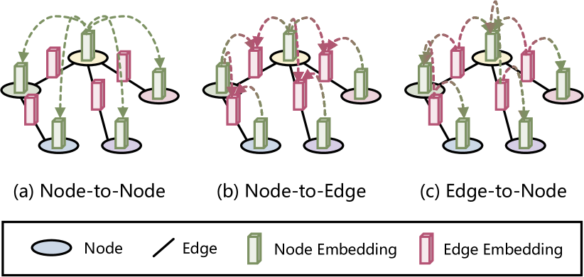
Figure 1: Illustration of the three ways for graph information propagation. Circles and black lines indicate nodes and edges, and green and pink cubes represent node embeddings and edge embeddings. Our GPTrans achieves better graph representation learning by explicitly constructing three ways for information propagation in the proposed Graph Propagation Attention (GPA) module, including (a) node-to-node, (b) node-to-edge, and (c) edge-to-node.

Although recent transformer-based methods report promising performance for graph representation learning, they still suffer the following problems. (1) Not explicitly employ the relationship among nodes and edges in the graph data. Recent transformer-based methods Cai and Lam (2020); Ying et al. (2021) only simply fuse nodes and edges information by using positional encodings. However, due to the complexity of graph structure, how to fully employ the relationship among nodes and edges for graph representation learning remains to be studied. (2) Inefficient dual-FFN structure in the transformer block. Recent works resort to the dual-path structure in the transformer block to incorporate the edge information. For instance, the Edge-augmented Graph Transformer (EGT) Hussain et al. (2021) adopted dual feed-forward networks (FFN) in the transformer block to update the edge embeddings, and let the structural information evolve from layer to layer. However, this paradigm learns the information of edges and nodes separately, which introduces more calculations and easily leads to the low efficiency of the model.

To overcome these issues, we propose an efficient and powerful transformer architecture for graph learning, termed Graph Propagation Transformer (GPTrans). A key design element of GPTrans is its Graph Propagation Attention (GPA) module. As illustrated in Figure 1, the GPA module propagates the information among the node embeddings and edge embeddings of the preceding layer by modeling three connections, i.e., node-to-node, node-to-edge, and edge-to-node, which significantly enhances modeling capability (see Table 1). This design benefits us no longer the need to maintain an FFN module specifically for edge embeddings, bringing higher efficiency than previous dual-FFN methods.

The contributions of our work are as follows:

$(1)$ We propose an effective Graph Propagation Transformer (GPTrans), which can better model the relationship among nodes and edges and represent the graph.

$(2)$ We introduce a novel attention mechanism in the transformer blocks, which explicitly passes the information among nodes and edges in three ways. These relationships play a critical role in graph representation learning.

$(3)$ Extensive experiments show that the proposed GPTrans model outperforms many state-of-the-art transformer-based methods on benchmark datasets with better performance.

2 Related Works

2.1 Transformer

The past few years have seen many transformer-based models designed for various language Vaswani et al. (2017); Radford et al. (2019); Brown et al. (2020) and vision tasks Parmar et al. (2018); Liu et al. (2021b). For example, in the field of vision, Dosovitskiy et al. Dosovitskiy et al. (2021) presented the Vision Transformer (ViT), which decomposed an image into a sequence of patches and captured their mutual relationships. However, training ViT on large-scale datasets can be computationally expensive. To address this issue, DeiT Touvron et al. (2021) proposed an efficient training strategy that enabled ViT to deliver exceptional performance even when trained on smaller datasets. Nevertheless, the complexity and performance of ViT remain challenging. To overcome these limitations, researchers further proposed many well-designed models Liu et al. (2021b); Wang et al. (2021, 2022a); Chen et al. (2023); Ji et al. (2023); Chen et al. (2022); Wang et al. (2022b).

Recently, the self-attention mechanism and transformer architecture have been gradually introduced into the graph representation learning tasks, such as graph-level prediction Ying et al. (2021); Hussain et al. (2021), producing competitive performance compared to the traditional GNN models. The early self-attention-based GNNs focused on adopting the attention mechanism to a local neighborhood of each node in a graph, or directly on the whole graph. For example, Graph Attention Network (GAT) Veličković et al. (2017) and Graph Transformer (GT) Dwivedi and Bresson (2020) utilized self-attention mechanisms as local constraints for the local neighborhood of each node. In contrast to employing local self-attention for graph learning, Graph-BERT Zhang et al. (2020) introduced the global self-attention mechanism in a revised transformer network to predict one masked node in a sampled subgraph.

In addition, several works have attempted to use the transformer architecture to tackle graph-related tasks directly. Two notable examples are Cai and Lam (2020) and Graphormer Ying et al. (2021). The former method adopted explicit relation encoding between nodes and integrated them into the encoder-decoder transformer network, to enable graph-to-sequence learning. The latter mainly regarded the structure and edges of the graph as the attention biases, which were incorporated into the transformer block. With the help of these attention biases, Graphormer achieved leading performance on graph-level prediction tasks (e.g., classification and regression on molecular graphs).

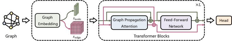
Figure 2: Overall architecture of GPTrans. It contains a graph embedding layer, $L$ transformer blocks, and a head. The graph embedding layer transforms the graph data into node embeddings $x_{\rm node}$ and edge embeddings $x_{\rm edge}$, as the input of the transformer blocks. Each transformer block comprises a Graph Propagation Attention (GPA) and a Feed-Forward Network (FFN). It is worth noting that we no longer need to maintain an FFN module specifically for edge embeddings due to the proposed GPA module, which improves the efficiency of our method. Finally, a head of two fully-connected layers is employed on the output embeddings for various graph tasks.

2.2 Graph Convolutional Network

Graph Convolutional Network (GCN) is a kind of deep neural network that extends the CNN from grid data (e.g., image and video) to graph-structured data. Generally speaking, GCN methods can be approximately divided into two types: spectral-based methods Bruna et al. (2013); Defferrard et al. (2016); Henaff et al. (2015); Kipf and Welling (2016) and non-spectral methods Chen et al. (2018); Gilmer et al. (2017); Scarselli et al. (2008); Veličković et al. (2017).

Spectral GCN methods are designed under the theory of spectral graphs. For instance, Spectral GCN Bruna et al. (2013) resorted to the Fourier basis of a graph to conduct convolution operation in the spectral domain, which is the first work on spectral graph CNNs. Based on Bruna et al. (2013), Defferrard et al. Defferrard et al. (2016) designed a strict control over the local support of filters and avoided an explicit use of the Graph Fourier basis in the convolution, which achieved better accuracy. Kipf and Welling Kipf and Welling (2016) adopted the first-order approximation of the spectral graph convolution to simplify commonly used GNN.

On the other hand, non-spectral methods directly define convolution operations on the graph data. GraphSage Hamilton et al. (2017) proposed learnable aggregator functions in the network to fuse neighbors’ information for effective graph representation learning. In GAT Veličković et al. (2017), different weight matrices are used for nodes with different degrees for graph representation learning. In addition, another line of GCN methods is mainly designed for specific graph-level tasks. For example, some techniques such as subsampling Chen et al. (2017) and inductive representation for a large graph Hamilton et al. (2017) have been introduced for better graph representative learning.

3 GPTrans

3.1 Overall Architecture

An overview of the proposed GPTrans framework is depicted in Figure 2. Specifically, it takes a graph $G=(V,E)$ as input, in which nodes $V=\{v_{1},v_{2},\dots,v_{n}\}$, $E$ indicates edges between nodes, and $n$ means the number of nodes. The pipeline of GPTrans can be divided into three parts: graph embedding, transformer blocks, and prediction head.

In the graph embedding layer, for each given graph $G$, we follow Ying et al. (2021); Hussain et al. (2021) to add a virtual node $[v_{0}]$ into $V$, to aggregate the information of the entire graph. Thus, the newly-generated node set with the virtual node is represented as $V^{\prime}=\{[v_{0}],v_{1},v_{2},\dots,v_{n}\}$, and the number of nodes is updated to $|V^{\prime}|=1+n$. For more adequate information propagation across the whole graph, each node and edge is treated as a token. In detail, we transform the input nodes into a sequence of node embeddings $x_{\rm node}\in\mathbb{R}^{(1+n)\times d_{1}}$, and encode the input edges into a tensor of edge embeddings $x_{\rm edge}\in\mathbb{R}^{(1+n)\times(1+n)\times d_{2}}$.

Then, $L$ transformer blocks with our re-designed self-attention operation (i.e., Graph Propagation Attention) are applied to node embeddings and edge embeddings. Both these embeddings are fed throughout all transformer blocks. After that, GPTrans generates the representation of each node and edge, in which the output embedding of the virtual node takes along the representation of the whole graph.

Finally, the head of our GPTrans is composed of two fully-connected (FC) layers. For graph-level tasks, we employ it on top of the output embedding of the virtual node. For node-level or edge(link)-level tasks, we apply it to the output node embeddings or edge embeddings. In summary, benefiting from the proposed novel Graph Propagation Attention, our GPTrans can better support various graph tasks with only a little additional computational cost compared to the previous method Graphormer Ying et al. (2021).

3.2 Graph Embedding

The role of the graph embedding layer is to transform the graph data as the input of transformer blocks. As we know, in addition to the nodes, edges also have rich structural information in many types of graphs, e.g., molecular graphs Hu et al. (2021) and social graphs Huang et al. (2022). Therefore, we encode both nodes and edges into embeddings to fully utilize the structure of the input graph.

For nodes in the graph, we transform each node into node embedding. Specifically, we follow Ying et al. (2021) to exploit the node attributes and the degree information, and add a virtual node $[v_{0}]$ into the graph to collect and propagate graph-level features. Without loss of generality, taking a directed graph as an example, its node embeddings $x_{\rm node}\in\mathbb{R}^{(1+n)\times d_{1}}$ can be expressed as:

$$x_{\rm node}=x_{\rm node\_attr}+x_{\rm deg^{-}}+x_{\rm deg^{+}},$$ (1)

where $x_{\rm node\_attr}$, $x_{\rm deg^{-}}$, and $x_{\rm deg^{+}}$ are embeddings encoded from node attributes, indegree, and outdegree statistics, respectively. $d_{1}$ is the dimension of node embeddings.

For edges in the graph, we also transform them into edge embeddings to help the learning of graph representation. In our implementation, the edge embeddings $x_{\rm edge}\in\mathbb{R}^{(1+n)\times(1+n)\times d_{2}}$ are defined as:

$$x_{\rm edge}=x_{\rm edge\_attr}+x_{\rm rel\_pos},$$ (2)

where $x_{\rm edge\_attr}$ is encoded from the edge attributes, and $x_{\rm rel\_pos}$ is a relative positional encoding that embeds the spatial location of node pairs. $d_{2}$ means the dimension of edge embeddings. We adopt the encoding of the shortest path distance by default following  Ying et al. (2021). In other words, for the position $(i,j)$, $x_{\rm edge}^{ij}\in\mathbb{R}^{d_{2}}$ represents the learned structural embedding of the edge (path) between node $v_{i}$ and node $v_{j}$ in the graph $G$.

It is worth noting that, unlike Graphormer Ying et al. (2021) that encodes edge attributes and spatial position as attention biases and shares them across all blocks, we optimize the edge embeddings $x_{\rm edge}$ in each transformer block by the proposed Graph Propagation Attention. Then, the updated edge embeddings are fed into the next block. Therefore, each block of our model could adaptively learn different ways to exploit edge features and propagate information. This more flexible way is beneficial for graph representation learning, which we will show in later experiments.

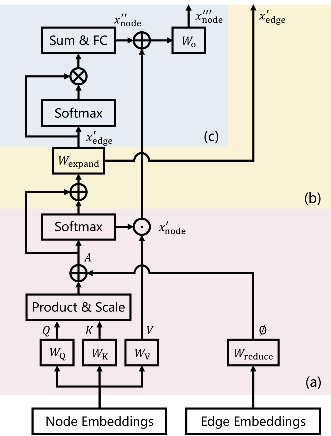
Figure 3: Illustration of Graph Propagation Attention. It explicitly builds three paths for information propagation among node embeddings and edge embeddings, including (a) node-to-node, (b) node-to-edge, and (c) edge-to-node.

3.3 Graph Propagation Attention

In recent years, many works Ying et al. (2021); Shi et al. (2022); Hussain et al. (2021) show global self-attention could serve as a flexible alternative to graph convolution and help better graph representation learning. However, most of them only consider part of the information propagation paths in graph, or introduce a lot of extra computational overhead to utilize edge information. For instance, Graphormer Ying et al. (2021) only used edge features as shared bias terms to refine the attention weights of nodes. GT Dwivedi and Bresson (2020) and EGT Hussain et al. (2021) designed dual-FFN networks to fuse edge features. Inspired by this, we introduce Graph Propagation Attention (GPA), as an efficient replacement for vanilla self-attention in graph transformers. With an affordable cost, it could support three types of propagation paths, including node-to-node, node-to-edge, and edge-to-node. For simplicity of description, we consider single-head self-attention in the following formulas.

3.3.1 Node-to-Node

Following common practices Ying et al. (2021); Shi et al. (2022); Hussain et al. (2021), we adopt global self-attention Vaswani et al. (2017) to perform node-to-node propagation. First, we use parameter matrices $W_{\rm Q}$, $W_{\rm K}$, and $W_{\rm V}\in\mathbb{R}^{d_{1}\times d_{1}}$ to project the node embeddings $x_{\rm node}$ to queries $Q$, keys $K$, and values $V$:

$$Q=x_{\rm node}W_{\rm Q},\ \ K=x_{\rm node}W_{\rm K},\ \ V=x_{\rm node}W_{\rm V}.$$ (3)

Unlike Graphormer Ying et al. (2021) that used shared attention biases in all blocks, we employ a parameter matrix $W_{\rm reduce}\in\mathbb{R}^{d_{2}\times{n_{\rm head}}}$ to predict layer-specific attention biases $\phi\in\mathbb{R}^{(1+n)\times(1+n)\times n_{\rm head}}$ from the edge embeddings $x_{\rm edge}$, which can be written as:

$$\phi=x_{\rm edge}W_{\rm reduce}.$$ (4)

Then, we add $\phi$ to the attention map of the query-key dot product and compute the output node embeddings $x^{\prime}_{\rm node}$. This process can be formulated as:

$$A=\frac{QK^{T}}{\sqrt{d_{\rm head}}}+\phi,\ \ \ \ x^{\prime}_{\rm node}={\rm softmax}(A)V,$$ (5)

where $A\in\mathbb{R}^{(1+n)\times(1+n)\times n_{\rm head}}$ represents the output attention map, and $d_{\rm head}$ refers to the dimension of each head. In summary, since $\phi$ are projected from higher dimensional edge embeddings by the learnable matrix, our attention map $A$ will have more flexible patterns to aggregate node features.

3.3.2 Node-to-Edge

To propagate node features to edges, we make some additional use of the attention map $A$. According to the definition of self-attention Vaswani et al. (2017), attention map $A$ captures the similarity between node embeddings. Therefore, considering both local and global connections, we add $A$ with its softmax confidence, and expand its dimension to as same as $x_{\rm edge}$ through the learnable matrix $W_{\rm expand}\in\mathbb{R}^{n_{\rm head}\times d_{2}}$. This operation is designed to perform explicit high-order spatial interactions, which can be written as follows:

$$x^{\prime}_{\rm edge}=(A+{\rm softmax}(A))W_{\rm expand}.$$ (6)

In this way, we achieve node-to-edge propagation without relying on an additional FFN module like GT Dwivedi and Bresson (2020) and EGT Hussain et al. (2021).

3.3.3 Edge-to-Node

In this part, we delve into the following question: How to generate dynamic weights for edge embeddings $x_{\rm edge}$ and fuse them into node embeddings $x_{\rm node}$? Due to the computational efficiency, we do not additionally perform attention operation, but directly apply the softmax function to the just generated $x^{\prime}_{\rm edge}\in\mathbb{R}^{(1+n)\times(1+n)\times d_{2}}$ in Eqn. 6 and calculate element-wise product with itself:

$$x^{\prime\prime}_{\rm node}={\rm FC}({\rm sum}(x^{\prime}_{\rm edge}\cdot{\rm softmax}(x^{\prime}_{\rm edge}),{\rm dim}=1)),$$ (7)

in which the fully-connected (FC) layer is used to align the dimension of edge embeddings and node embeddings. This process again explicitly introduces high-order spatial interactions. Finally, we add these two types of node embeddings, and employ a learnable matrix $W_{\rm O}\in\mathbb{R}^{d_{1}\times d_{1}}$ to fuse them. Then we have the updated node embeddings:

$$x^{\prime\prime\prime}_{\rm node}=(x^{\prime}_{\rm node}+x^{\prime\prime}_{\rm node})W_{\rm O}.$$ (8)

3.3.4 GPA in Transformer Blocks

Equipped with our proposed GPA module, the block of our GPTrans can be calculated as follows:

$$\hat{x}^{l}_{\rm node},x^{l}_{\rm edge}\mathrel{{+}{=}}{\rm GPA}({\rm LN}(x^{l-1}_{\rm node}),x^{l-1}_{\rm edge}),$$ (9)

$$x^{l}_{\rm node}={\rm FFN}({\rm LN}(\hat{x}^{l}_{\rm node}))+\hat{x}^{l}_{\rm node},$$ (10)

where $\rm LN(\cdot)$ means layer normalization Ba et al. (2016). $\hat{x}^{l}_{\rm node}$ and $x^{l}_{\rm edge}$ denote the output node embeddings and edge embeddings of the GPA module for block $l$. And $x^{l}_{\rm node}$ represents the output node embeddings of the FFN module. Overall, our GPA module effectively extends the ability of our GPTrans to various graph tasks, but only introduces a small amount of extra overhead compared with previous methods Hussain et al. (2021); Ying et al. (2021).

3.4 Architecture Configurations

		PCQM4M$\downarrow$		PCQM4Mv2$\downarrow$
Model	#Param	Validate	Test	Validate	Test-dev
Non-transformer-based Methods
GCN	2.0M	0.1684	0.1838	0.1379	0.1398
GIN	3.8M	0.1536	0.1678	0.1195	0.1218
GCN-VN	4.9M	0.1510	0.1579	0.1153	0.1152
GIN-VN	6.7M	0.1396	0.1487	0.1083	0.1084
GINE-VN	13.2M	0.1430	$-$	$-$	$-$
DeeperGCN-VN	25.5M	0.1398	$-$	$-$	$-$
Transformer-based Methods
GPS-Small	6.2M	$-$	$-$	0.0938	$-$
GPTrans-T (ours)	6.6M	0.1179	$-$	0.0833	$-$
Graphormer-S	12.5M	0.1264	$-$	0.0910	$-$
EGT-Small	11.5M	0.1260	$-$	0.0899	$-$
GPS-Medium	19.4M	$-$	$-$	0.0858	$-$
GPTrans-S (ours)	13.6M	0.1162	$-$	0.0823	$-$
TokenGT	48.5M	$-$	$-$	0.0910	$-$
Graphormer-B	47.1M	0.1234	$-$	0.0906	$-$
GRPE-Standard	46.2M	0.1225	$-$	0.0890	0.0898
EGT-Medium	47.4M	0.1224	$-$	0.0881	$-$
GPTrans-B (ours)	45.7M	0.1153	$-$	0.0813	$-$
GT-Wide	83.2M	0.1408	$-$	$-$	$-$
GraphormerV2-L	159.3M	0.1228	$-$	0.0883	$-$
EGT-Large	89.3M	$-$	$-$	0.0869	0.0872
EGT-Larger	110.8M	$-$	$-$	0.0859	$-$
GRPE-Large	118.3M	$-$	$-$	0.0867	0.0876
GPS-Deep	138.1M	$-$	$-$	0.0852	0.0862
GPTrans-L (ours)	86.0M	0.1151	$-$	0.0809	0.0821

Table 1: Results on PCQM4M and PCQM4Mv2. The metric is the Mean Absolute Error (MAE), and the lower the better. “$-$” denotes results are not available since the labels of test and test-dev sets are not public. Highlighted are the best results for each model size.

We build five variants of the proposed model with different model sizes, namely GPTrans-Nano, Tiny, Small, Base, and Large. Note that the number of parameters of our GPTrans is similar to Graphormer Ying et al. (2021) and EGT Hussain et al. (2021). The dimension of each head is set to 10 for our nano model, and 32 for others. Following common practices, the expansion ratio of the FFN module is $\alpha=1$ for all model variants. The architecture hyper-parameters of these five models are as follows:

• GPTrans-Nano: $d_{1}=80$, $d_{2}=40$, layer number = $12$

• GPTrans-Tiny: $d_{1}=256$, $d_{2}=32$, layer number = $12$

• GPTrans-Small: $d_{1}=384$, $d_{2}=48$, layer number = $12$

• GPTrans-Base: $d_{1}=608$, $d_{2}=76$, layer number = $18$

• GPTrans-Large: $d_{1}=736$, $d_{2}=92$, layer number = $24$

The model size and performance of the model variants on the large-scale PCQM4M and PCQM4Mv2 benchmarks Hu et al. (2021) are listed in Table 1, and the analysis of model efficiency is provided in Table 6. More detailed model configurations are presented in the appendix.

Model	#Param	Test AP(%)$\uparrow$
Non-transformer-based Methods
DeeperGCN-VN-FLAG Li et al. (2020)	5.6M	28.42 $\pm$ 0.43
PNA Corso et al. (2020)	6.5M	28.38 $\pm$ 0.35
DGN Beaini et al. (2021)	6.7M	28.85 $\pm$ 0.30
GINE-VN Brossard et al. (2020)	6.1M	29.17 $\pm$ 0.15
PHC-GNN Le et al. (2021)	1.7M	29.47 $\pm$ 0.26
GIN-VN† Xu et al. (2018)	3.4M	29.02 $\pm$ 0.17
Transformer-based Methods
GRPE-Standard† Park et al. (2022)	46.2M	30.77 $\pm$ 0.07
GPTrans-B† (ours)	45.7M	31.15 $\pm$ 0.16
GRPE-Large† Park et al. (2022)	118.3M	31.50 $\pm$ 0.10
Graphormer-L† Ying et al. (2021)	119.5M	31.39 $\pm$ 0.32
EGT-Larger† Hussain et al. (2021)	110.8M	29.61 $\pm$ 0.24
GPTrans-L† (ours)	86.0M	32.43 $\pm$ 0.22

Table 2: Results on MolPCBA. ^† indicates the model is pre-trained on PCQM4M or PCQM4Mv2. The higher the better. Highlighted are the best results for each model size.

Model	#Param	Test AUC(%)$\uparrow$
Non-transformer-based Methods
DeeperGCN-FLAG Li et al. (2020)	532K	79.42 $\pm$ 1.20
PNA Corso et al. (2020)	326K	79.05 $\pm$ 1.32
DGN Beaini et al. (2021)	110K	79.70 $\pm$ 0.97
PHC-GNN Le et al. (2021)	114K	79.34 $\pm$ 1.16
GIN-VN† Xu et al. (2018)	3.3M	77.80 $\pm$ 1.82
Transformer-based Methods
Graphormer-B† Ying et al. (2021)	47.0M	80.51 $\pm$ 0.53
EGT-Larger† Hussain et al. (2021)	110.8M	80.60 $\pm$ 0.65
GRPE-Standard† Park et al. (2022)	46.2M	81.39 $\pm$ 0.49
GPTrans-B† (ours)	45.7M	81.26 $\pm$ 0.32

Table 3: Results on MolHIV. ^† indicates the model is pre-trained on PCQM4M or PCQM4Mv2. The higher the better. Highlighted are the best results.

4 Experiments

		ZINC	PATTERN	CLUSTER	TSP
Model	#Param	Test MAE$\downarrow$	Accuracy(%)$\uparrow$	Accuracy(%)$\uparrow$	F1-Score$\uparrow$
Non-transformer-based Methods
GCN Kipf and Welling (2016)	505K	0.367 $\pm$ 0.011	71.892 $\pm$ 0.334	68.498 $\pm$ 0.976	$-$
GraphSage Hamilton et al. (2017)	505K	0.398 $\pm$ 0.002	50.492 $\pm$ 0.001	63.884 $\pm$ 0.110	$-$
GIN Xu et al. (2018)	510K	0.526 $\pm$ 0.051	85.387 $\pm$ 0.136	64.716 $\pm$ 1.553	$-$
GAT Veličković et al. (2017)	531K	0.384 $\pm$ 0.007	78.271 $\pm$ 0.186	70.587 $\pm$ 0.447	$-$
GatedGCN Bresson and Laurent (2017)	505K	0.214 $\pm$ 0.013	86.508 $\pm$ 0.085	76.082 $\pm$ 0.196	0.838 $\pm$ 0.002
PNA Corso et al. (2020)	387K	0.142 $\pm$ 0.010	$-$	$-$	$-$
Transformer-based Methods
GT Dwivedi and Bresson (2020)	589K	0.226 $\pm$ 0.014	84.808 $\pm$ 0.068	73.169 $\pm$ 0.622	$-$
SAN Kreuzer et al. (2021)	509K	0.139 $\pm$ 0.006	86.581 $\pm$ 0.037	76.691 $\pm$ 0.650	$-$
Graphormer-Slim Ying et al. (2021)	489K	0.122 $\pm$ 0.006	86.650 $\pm$ 0.033	74.660 $\pm$ 0.236	0.698 $\pm$ 0.007
EGT Hussain et al. (2021)	500K	0.108 $\pm$ 0.009	86.821 $\pm$ 0.020	79.232 $\pm$ 0.348	0.853 $\pm$ 0.001
GPS Rampášek et al. (2022)	424K	0.070 $\pm$ 0.004	86.685 $\pm$ 0.059	78.016 $\pm$ 0.180	$-$
GPTrans-Nano (ours)	554K	0.077 $\pm$ 0.009	86.731 $\pm$ 0.085	78.069 $\pm$ 0.154	0.832 $\pm$ 0.004

Table 4: Results on four benchmarking datasets, including graph regression (ZINC), node classification (PATTERN and CLUSTER), and edge classification (TSP) tasks. The arrow next to the metric means higher or lower is better. “$-$” denotes the results are not available. Highlighted are the top first and second results.

4.1 Graph-Level Tasks

4.1.1 Datasets

We verify the following graph-level tasks:

(1) PCQM4M Hu et al. (2021) is a quantum chemistry dataset that includes 3.8 million molecular graphs and a total of 53 million nodes. The task is to regress a DFT-calculated quantum chemical property, e.g., HOMO-LUMO energy gap.

(2) PCQM4Mv2 Hu et al. (2021) is an updated version of PCQM4M, in which the number of molecules slightly decreased, and some of the graphs are revised.

(3) MolHIV Hu et al. (2020) is a small-scale molecular property prediction dataset. It has $41,127$ graphs with a total of $1,048,738$ nodes and $1,130,993$ edges.

(4) MolPCBA Hu et al. (2020) is another property prediction dataset, which is larger than MolHIV. It contains $437,929$ graphs with $11,386,154$ nodes and $12,305,805$ edges.

(5) ZINC Dwivedi et al. (2020) is a popular real-world molecular dataset for graph property regression. It has $10,000$ train, $1,000$ validation, and $1,000$ test graphs.

4.1.2 Settings

For the large-scale PCQM4M and PCQM4Mv2 datasets, we use AdamW Loshchilov and Hutter (2018) with an initial learning rate of 1e-3 as the optimizer. Following common practice, we adopt a cosine decay learning rate scheduler with a 20-epoch warmup. All models are trained for 300 epochs with a total batch size of 1024. When fine-tuning the MolHIV and MolPCBA datasets, we load the PCQM4Mv2 pre-trained weights as initialization. For the ZINC dataset, we train our GPTrans-Nano model from scratch. More detailed training strategies are provided in the appendix.

4.1.3 Results

First, we benchmark our GPTrans method on PCQM4M and PCQM4Mv2, two datasets from OGB large-scale challenge Hu et al. (2021). We mainly compare our GPTrans against a set of representative transformer-based methods, including GT Dwivedi and Bresson (2020), Graphormer Ying et al. (2021), GRPE Park et al. (2022), EGT Hussain et al. (2021), GPS Rampášek et al. (2022), and TokenGT Kim et al. (2022). As reported in Table 1, our method yields the state-of-the-art validate MAE score on both datasets across different model complexities.

Further, we take the PCQM4Mv2 pre-trained weights as the initialization and fine-tune our models on the OGB molecular datasets MolPCBA and MolHIV, to verify the transfer learning capability of GPTrans. All experiments are performed five times with different random seeds, and we report the mean and standard deviation of the results. From Table 2 and 3, we can see that GPTrans outperforms many strong counterparts, such as GRPE Park et al. (2022), EGT Hussain et al. (2021), and Graphormer Ying et al. (2021).

Moreover, we follow previous methods Park et al. (2022); Ying et al. (2021) to train the GPTrans-Nano model with about 500K parameters on the ZINC subset from scratch. As demonstrated in Table 4, our model achieves a promising test MAE of 0.077 $\pm$ 0.009, bringing 36.9% relative MAE decline compared to Graphormer Ying et al. (2021). The above inspiring results show that the proposed GPTrans performs well on graph-level tasks.

4.2 Node-Level Tasks

4.2.1 Datasets

PATTERN and CLUSTER Dwivedi et al. (2020) are both synthetic datasets for node classification. Specifically, PATTERN has $10,000$ training, $2,000$ validation, and $2,000$ test graphs, and CLUSTER contains $10,000$ training, $1,000$ validation, and $1,000$ test graphs.

4.2.2 Settings

For the PATTERN and CLUSTER datasets, we train our GPTrans-Nano up to 1000 epochs with a batch size of 256. We employ the AdamW Loshchilov and Hutter (2018) optimizer with a 20-epoch warmup. The learning rate is initialized to 5e-4, and is declined by a cosine scheduler. More training details can be found in the appendix.

4.2.3 Results

In this part, we compare our GPTrans-Nano with various GCN variants and recent graph transformers. As shown in Table 4, our GPTrans-Nano produces the promising accuracy of 86.731 $\pm$ 0.085$\%$ and 78.069 $\pm$ 0.154$\%$ on the PATTERN and CLUSTER datasets, respectively. These results outperform many Convolutional/Message-Passing Graph Neural Networks by large margins, showing that the proposed GPTrans can serve as an alternative to traditional GCNs for node-level tasks. Moreover, we find that our method exceeds Graphormer Ying et al. (2021) on the CLUSTER dataset by significant gaps of 3.4% accuracy, which suggests that the three propagation ways explicitly constructed in the GPA module are also helpful for node-level tasks.

4.3 Edge-Level Tasks

4.3.1 Datasets

TSP Dwivedi et al. (2020) is a dataset for the Traveling Salesman Problem, which is an NP-hard combinatorial optimization problem. The problem is reduced to a binary edge classification task, where edges in the TSP tour have positive labels. TSP dataset has $10,000$ training, $1,000$ validation, and $1,000$ test graphs.

Model	#Param	FLOPs	Validate MAE$\downarrow$
Baseline (Graphormer-S)	12.5M	0.399G	0.0928
+ Node-to-Node	13.3M	0.402G	0.0874
++ Node-to-Edge	13.3M	0.405G	0.0865
+++ Edge-to-Node	13.5M	0.417G	0.0854
GPTrans-Swider	13.5M	0.417G	0.0854
GPTrans-Sdeeper (ours)	13.6M	0.472G	0.0835

Table 5: Ablation studies of GPTrans. FLOPs is calculated using a graph with 20 nodes. We build our baseline based on Graphormer-S with a shorter schedule of 100 epochs, and decline its validate MAE on the PCQM4Mv2 dataset from 0.0928 to 0.0854 by gradually introducing our GPA module. Moreover, we find that the deeper model outperforms the wider model with a similar number of parameters.

4.3.2 Settings

We experiment on the TSP dataset in a similar setting to that used in the PATTERN and CLUSTER datasets. Details are shown in the appendix.

4.3.3 Results

Table 4 compares the edge classification performance of our GPTrans-Nano model and previously transformer-based methods on the TSP dataset. We observe GPTrans can outperform Graphormer Ying et al. (2021) with a large margin and is comparable with EGT Hussain et al. (2021), showing that the proposed GPA module design is competitive when used for edge-level tasks. By applying the GPA module, we avoid designing an inefficient dual-FFN network, which boosts the efficiency of our method. We will analyze the efficiency of GPTrans in detail in Section 4.4.

4.4 Ablation Study

We conduct several ablation studies on the PCQM4Mv2 Hu et al. (2021) dataset, to validate the effectiveness of each key design in our GPTrans. Due to the limited computational resources, we adopt GPTrans-S as the base model, and train it with a shorter schedule of 100 epochs. Other settings are the same as described in Section 4.1.

4.4.1 Graph Propagation Attention

To investigate the contribution of each key design in our GPA module, we gradually extend the Graphormer baseline Ying et al. (2021) to our GPTrans. As shown in Table 5, the model gives the best performance when all three information propagation paths are introduced. It is worth noting that the improvement from our node-to-node propagation is most significant, thanks to learning the attention biases for a particular layer rather than sharing them across all layers. In summary, our proposed GPA module collectively brings a large gain to Graphormer, i.e., 8.0% relative validate MAE decline on the PCQM4Mv2 dataset.

4.4.2 Deeper vs. Wider

Here we explore the question of whether the transformers for graph representation learning should go deeper or wider. For fair comparisons, we build a deeper but thinner model under comparable parameter numbers, by increasing the depth from 6 to 12 layers and decreasing the width from 512 to 384 dimensions. As reported in Table 5, the validate MAE of the PCQM4Mv2 dataset is declined from 0.0854 to 0.0835 by the deeper model, which shows that depth is more important than width for graph transformers. Based on this observation, we prefer to develop GPTrans with a large model depth.

		Train	Inference	PCQM4Mv2
Model	#Param	(min / ep.)	(graph / s)	Validate MAE$\downarrow$
EGT-Small	11.5M	7.6	10291.8	0.0899
GPTrans-S	13.6M	5.5	11391.2	0.0823
EGT-Medium	47.4M	11.3	4840.8	0.0881
GPTrans-B	45.7M	7.7	6670.6	0.0813
EGT-Large	89.3M	15.5	3759.4	0.0869
GPTrans-L	86.0M	9.6	4193.4	0.0809

Table 6: Efficiency analysis of GPTrans. These experiments are conducted with PyTorch1.12 and CUDA11.3. Training time is measured on 8 A100 GPUs with half-precision training, and the inference throughput is tested on a single A100 GPU.

4.4.3 Efficiency Analysis

As shown in Table 6, we benchmark the training time and inference throughputs of our GPTrans and EGT Hussain et al. (2021). Specifically, we employ PyTorch1.12 and CUDA11.3 to perform these experiments. For a fair comparison, the training time of these two methods is measured using 8 Nvidia A100 GPUs with half-precision training and a total batch size of 1024. The inference throughputs of PCQM4Mv2 models in Table 6 are tested using an A100 GPU with a batch size of 128, where our GPTrans is slightly faster in inference than EGT under a similar number of parameters. This preliminary study shows a good signal that the proposed GPTrans, equipped with the GPA module, could be an efficient model for graph representation learning.

5 Conclusion

This paper aims for graph representation learning with a Graph Propagation Transformer (GPTrans), which explores the information propagation among nodes and edges in a graph when establishing the self-attention mechanism in the transformer block. Especially in the GPTrans, we propose a Graph Propagation Attention (GPA) mechanism to explicitly pass the information among nodes and edges in three ways, i.e., node-to-node, node-to-edge, and edge-to-node, which is essential for learning graph-structured data. Extensive comparisons with state-of-the-art methods on several benchmark datasets demonstrate the superior capability of the proposed GPTrans with better performance.

Contribution Statement

Zhe Chen and Hao Tan contributed equally to this work.

Dataset	#Graphs	Avg. Nodes	Avg. Edges	Task Type	Metric
PCQM4M Hu et al. (2021)	3,803,453	14.1	14.6	Graph Regression	Mean Absolute Error
PCQM4Mv2 Hu et al. (2021)	3,746,619	14.1	14.6	Graph Regression	Mean Absolute Error
MolHIV Hu et al. (2021)	41,127	25.5	27.5	Graph Classification	ROC-AUC
MolPCBA Hu et al. (2021)	437,929	26.0	28.1	Graph Classification	Average Precision
ZINC Dwivedi et al. (2020)	12,000	23.2	49.8	Graph Regression	Mean Absolute Error
PATTERN Dwivedi et al. (2020)	14,000	117.5	4749.2	Node Classification	Accuracy
CLUSTER Dwivedi et al. (2020)	12,000	117.2	4301.7	Node Classification	Accuracy
TSP Dwivedi et al. (2020)	12,000	275.6	6894.0	Edge Classification	F1 Score

Table 7: Overview of the datasets used in our experiments, covering graph-level, node-level, and edge-level tasks.

Appendix A Datasets

In Table 7, we list the information of the datasets used for training and evaluation. Next, we describe them in detail.

PCQM4M Hu et al. (2021) is a large-scale molecular dataset that includes 3.8 million molecular graphs and a total of 53 million nodes. The task is to regress a DFT-calculated quantum chemical property, e.g., the HOMO-LUMO energy gap of a given molecule. The HOMO-LUMO gap is one of the most practically relevant quantum chemical properties of molecules. Using efficient and accurate deep learning models to approximate DFT enables diverse downstream applications, e.g., drug discovery.

PCQM4Mv2 Hu et al. (2021) is an updated version of PCQM4M. In PCQM4Mv2, the number of molecules slightly decreased, and some of the graphs were revised.

MolHIV Hu et al. (2020) is a small-scale molecular property prediction dataset, and is part of the Open Graph Benchmark Hu et al. (2021). Specifically, the MolHIV dataset is a molecular tree-like dataset consisting of $41,127$ graphs, with an average number of 25.5 nodes and 27.5 edges per graph. The task is to predict whether a molecule inhibits HIV virus replication.

MolPCBA Hu et al. (2020) is a medium-scale molecular property prediction dataset featuring 128 imbalanced binary classification tasks. It contains $437,929$ graphs with $11,386,154$ nodes and $12,305,805$ edges.

ZINC Dwivedi et al. (2020) is the most popular real-world molecular dataset to predict graph property regression for constrained solubility, which is an important chemical property for designing generative GNNs for molecules. To be specific, ZINC has 12,000 graphs, usually used as a benchmark for evaluating GNN performances.

PATTERN and CLUSTER Dwivedi et al. (2020) are node classification datasets synthesized with Stochastic Block Model. In PATTERN, the task is to tell if a node belongs to one of the randomly generated 100 patterns in a large graph. In CLUSTER, every graph comprises 6 SBM clusters, and each graph only contains one labeled node with a feature value set to the cluster ID. The task is to predict the cluster ID of every node.

TSP Dwivedi et al. (2020) is an edge classification dataset, where edges in graphs have binary labels corresponding to the TSP tour of that graph. Specifically, the label of an edge is set to 1 if it belongs to the TSP tour and is set to 0 otherwise. The TSP problem is one of the NP-hard combinatorial optimization problems, and the utilization of machine learning methods to solve them has been intensively researched in recent years.

Hyper-parameter	Nano/Tiny/Small/Base/Large
#Layers	12/12/12/18/24
Dimension $d_{1}$	80/256/384/608/736
Dimension $d_{2}$	40/32/48/76/92
FFN Ratio $\alpha$	1.0
#Attention Head	8/8/12/19/23
Dimension of Each Head	10/32/32/32/32
Layer Scale	✗/✓/✓/✓/✓

Table 8: Model configurations of GPTrans. We build 5 variants of GPTrans with different model sizes, namely GPTrans-Nano, Tiny, Small, Base, and Large.

Hyper-parameter	Tiny/Small/Base/Large
FFN Dropout	0.1/0.1/0.1/0.2
Embedding Dropout	0.1/0.1/0.1/0.2
Attention Dropout	0.1/0.1/0.1/0.2
Drop Path Rate	0.1/0.1/0.2/0.4
Max Epochs	300
Warm-up Epochs	20
Peak Learning Rate	1e-3
Batch Size	1024
Learning Rate Decay	Cosine
Adam $\epsilon$	1e-8
Adam $(\beta_{2},\beta_{2})$	(0.9, 0.999)
Weight Decay	0.05
EMA	✓

Table 9: Hyper-parameters on PCQM4M and PCQM4Mv2.

Appendix B Model Configurations

We build 5 variants of GPTrans with different model sizes, called GPTrans-Nano, Tiny (T), Small (S), Base (B), and Large (L). Specifically, we follow EGT Hussain et al. (2021) and Graphormer Ying et al. (2021) to scale up our GPTrans. The dimension of each head is set to 10 for our nano model, and 32 for others. The expansion ratio of the FFN modules is $\alpha=1$ for all model variants. Other hyper-parameters of these models can be found in Table 8.

Appendix C Training Strategies

C.1 PCQM4M and PCQM4Mv2

We first report the hyper-parameters of the experiments on PCQM4M and PCQM4Mv2 datasets in Table 9. Empirically, for our GPTrans-T/S/B models, the dropout ratios of FFN, embedding, and attention are set to 0.1 by default, while for the GPTrans-L model, it is set to 0.2. Besides, the drop path rates are set to 0.1/0.1/0.2/0.4 for these variants along with the model scaling up.

Dataset	MolHIV	MolPCBA
Model	Base	Base/Large
Initialization	PCQM4Mv2	PCQM4Mv2
FFN Dropout	0.1	0.1/0.2
Embedding Dropout	0.1	0.1/0.2
Attention Dropout	0.1	0.1/0.2
Drop Path Rate	0.1	0.1/0.4
Max Epochs	10	50
Peak Learning Rate	2e-4	4e-4
Min Learning Rete	1e-4	1e-9
Batch Size	128	128
Warm-up Epochs	1	1
Learning Rate Decay	Cosine	Cosine
Adam $\epsilon$	1e-8	1e-8
Adam $(\beta_{2},\beta_{2})$	(0.9, 0.999)	(0.9, 0.999)
Weight Decay	0.0	0.0
EMA	✓	✓

Table 10: Hyper-parameters on MolHIV and MolPCBA.

Dataset	ZINC/PATTERN/CLUSTER/TSP
FFN Dropout	0.3
Embedding Dropout	0.3
Attention Dropout	0.5
Drop Path Rate	0.3
Max Epochs	10000/1000/1000/1000
Peak Learning Rate	5e-4
Batch Size	256/256/256/32
Warm-up Epochs	20
Learning Rate Decay	Cosine
Weight Decay	0.05
EMA	✓

Table 11: Hyper-parameters on 4 benchmarking datasets.

C.2 MolHIV and MolPCBA

We fine-tune our GPTrans-B on MolHIV and GPTrans-B/L on MolPCBA datasets, and load the PCQM4Mv2 pre-trained weights as initialization. Most of the hyper-parameters are consistent with the pre-training stage, see Table 10 for details. In addition, each experiment in these datasets is run 5 times with 5 different random seeds, and the results are used to calculate the mean and standard deviations of the metric.

C.3 ZINC/PATTERN/CLUSTER/TSP

For the 4 benchmarking datasets from Dwivedi et al. (2020), i.e., ZINC, PATTERN, CLUSTER, and TSP, we employ the AdamW optimizer Loshchilov and Hutter (2018) with a 20-epoch warmup, and reduce the learning rate by a cosine learning rate scheduler. The dropout ratios of FFN, embedding, and attention are set to 0.3, 0.3, and 0.5, respectively. The weight decay is set to 0.05. Each experiment is run 5 times with 5 different random seeds, and the results are used to calculate the mean and standard deviations of the metric.

References

- Ba et al. [2016] Jimmy Lei Ba, Jamie Ryan Kiros, and Geoffrey E Hinton. Layer normalization. arXiv preprint arXiv:1607.06450, 2016.
- Beaini et al. [2021] Dominique Beaini, Saro Passaro, Vincent Létourneau, Will Hamilton, Gabriele Corso, and Pietro Liò. Directional graph networks. In Proceedings of International Conference on Machine Learning, pages 748–758. PMLR, 2021.
- Bresson and Laurent [2017] Xavier Bresson and Thomas Laurent. Residual gated graph convnets. arXiv preprint arXiv:1711.07553, 2017.
- Brossard et al. [2020] Rémy Brossard, Oriel Frigo, and David Dehaene. Graph convolutions that can finally model local structure. arXiv preprint arXiv:2011.15069, 2020.
- Brown et al. [2020] Tom Brown, Benjamin Mann, Nick Ryder, Melanie Subbiah, Jared D Kaplan, Prafulla Dhariwal, Arvind Neelakantan, Pranav Shyam, Girish Sastry, Amanda Askell, et al. Language models are few-shot learners. Advances in Neural Information Processing Systems, 33:1877–1901, 2020.
- Bruna et al. [2013] Joan Bruna, Wojciech Zaremba, Arthur Szlam, and Yann LeCun. Spectral networks and locally connected networks on graphs. arXiv preprint arXiv:1312.6203, 2013.
- Cai and Lam [2020] Deng Cai and Wai Lam. Graph transformer for graph-to-sequence learning. In Proceedings of the AAAI Conference on Artificial Intelligence, pages 7464–7471, 2020.
- Chen et al. [2017] Jianfei Chen, Jun Zhu, and Le Song. Stochastic training of graph convolutional networks with variance reduction. arXiv preprint arXiv:1710.10568, 2017.
- Chen et al. [2018] Jie Chen, Tengfei Ma, and Cao Xiao. Fastgcn: fast learning with graph convolutional networks via importance sampling. In Proceedings of International Conference on Learning Representations, 2018.
- Chen et al. [2020] Deli Chen, Yankai Lin, Wei Li, Peng Li, Jie Zhou, and Xu Sun. Measuring and relieving the over-smoothing problem for graph neural networks from the topological view. In Proceedings of the AAAI Conference on Artificial Intelligence, pages 3438–3445, 2020.
- Chen et al. [2022] Guo Chen, Sen Xing, Zhe Chen, Yi Wang, Kunchang Li, Yizhuo Li, Yi Liu, Jiahao Wang, Yin-Dong Zheng, Bingkun Huang, et al. Internvideo-ego4d: A pack of champion solutions to ego4d challenges. arXiv preprint arXiv:2211.09529, 2022.
- Chen et al. [2023] Zhe Chen, Yuchen Duan, Wenhai Wang, Junjun He, Tong Lu, Jifeng Dai, and Yu Qiao. Vision transformer adapter for dense predictions. In International Conference on Learning Representations, 2023.
- Corso et al. [2020] Gabriele Corso, Luca Cavalleri, Dominique Beaini, Pietro Liò, and Petar Veličković. Principal neighbourhood aggregation for graph nets. Proceedings of Advances in Neural Information Processing Systems, 33:13260–13271, 2020.
- Defferrard et al. [2016] Michaël Defferrard, Xavier Bresson, and Pierre Vandergheynst. Convolutional neural networks on graphs with fast localized spectral filtering. In Proceedings of Advances in Neural Information Processing Systems, 2016.
- Dosovitskiy et al. [2021] Alexey Dosovitskiy, Lucas Beyer, Alexander Kolesnikov, Dirk Weissenborn, Xiaohua Zhai, Thomas Unterthiner, Mostafa Dehghani, Matthias Minderer, Georg Heigold, Sylvain Gelly, et al. An image is worth 16x16 words: Transformers for image recognition at scale. In Proceedings of International Conference on Machine Learning, 2021.
- Dwivedi and Bresson [2020] Vijay Prakash Dwivedi and Xavier Bresson. A generalization of transformer networks to graphs. arXiv preprint arXiv:2012.09699, 2020.
- Dwivedi et al. [2020] Vijay Prakash Dwivedi, Chaitanya K Joshi, Thomas Laurent, Yoshua Bengio, and Xavier Bresson. Benchmarking graph neural networks. arXiv preprint arXiv:2003.00982, 2020.
- Gilmer et al. [2017] Justin Gilmer, Samuel S Schoenholz, Patrick F Riley, Oriol Vinyals, and George E Dahl. Neural message passing for quantum chemistry. In Proceedings of International Conference on Machine Learning, pages 1263–1272, 2017.
- Hamilton et al. [2017] Will Hamilton, Zhitao Ying, and Jure Leskovec. Inductive representation learning on large graphs. In Proceedings of Advances in Neural Information Processing Systems, 2017.
- Henaff et al. [2015] Mikael Henaff, Joan Bruna, and Yann LeCun. Deep convolutional networks on graph-structured data. arXiv preprint arXiv:1506.05163, 2015.
- Hu et al. [2020] Weihua Hu, Matthias Fey, Marinka Zitnik, Yuxiao Dong, Hongyu Ren, Bowen Liu, Michele Catasta, and Jure Leskovec. Open graph benchmark: Datasets for machine learning on graphs. In Proceedings of Advances in Neural Information Processing Systems, 2020.
- Hu et al. [2021] Weihua Hu, Matthias Fey, Hongyu Ren, Maho Nakata, Yuxiao Dong, and Jure Leskovec. Ogb-lsc: A large-scale challenge for machine learning on graphs. In Proceedings of Conference on Neural Information Processing Systems Datasets and Benchmarks Track, 2021.
- Huang et al. [2022] Xuanwen Huang, Yang Yang, Yang Wang, Chunping Wang, Zhisheng Zhang, Jiarong Xu, and Lei Chen. Dgraph: A large-scale financial dataset for graph anomaly detection. arXiv preprint arXiv:2207.03579, 2022.
- Hussain et al. [2021] Md Shamim Hussain, Mohammed J Zaki, and Dharmashankar Subramanian. Global self-attention as a replacement for graph convolution. arXiv preprint arXiv:2108.03348, 2021.
- Ji et al. [2023] Yuanfeng Ji, Zhe Chen, Enze Xie, Lanqing Hong, Xihui Liu, Zhaoqiang Liu, Tong Lu, Zhenguo Li, and Ping Luo. Ddp: Diffusion model for dense visual prediction. arXiv preprint arXiv:2303.17559, 2023.
- Kim et al. [2022] Jinwoo Kim, Tien Dat Nguyen, Seonwoo Min, Sungjun Cho, Moontae Lee, Honglak Lee, and Seunghoon Hong. Pure transformers are powerful graph learners. arXiv preprint arXiv:2207.02505, 2022.
- Kipf and Welling [2016] Thomas N Kipf and Max Welling. Semi-supervised classification with graph convolutional networks. arXiv preprint arXiv:1609.02907, 2016.
- Kreuzer et al. [2021] Devin Kreuzer, Dominique Beaini, Will Hamilton, Vincent Létourneau, and Prudencio Tossou. Rethinking graph transformers with spectral attention. In Proceedings of Advances in Neural Information Processing Systems, pages 21618–21629, 2021.
- Le et al. [2021] Tuan Le, Marco Bertolini, Frank Noé, and Djork-Arné Clevert. Parameterized hypercomplex graph neural networks for graph classification. In Proceedings of International Conference on Artificial Neural Networks, pages 204–216, 2021.
- Li et al. [2020] Guohao Li, Chenxin Xiong, Ali Thabet, and Bernard Ghanem. Deepergcn: All you need to train deeper gcns. arXiv preprint arXiv:2006.07739, 2020.
- Liu et al. [2021a] Meng Liu, Zhengyang Wang, and Shuiwang Ji. Non-local graph neural networks. IEEE Transactions on Pattern Analysis and Machine Intelligence, 2021.
- Liu et al. [2021b] Ze Liu, Yutong Lin, Yue Cao, Han Hu, Yixuan Wei, Zheng Zhang, Stephen Lin, and Baining Guo. Swin transformer: Hierarchical vision transformer using shifted windows. In Proceedings of the IEEE International Conference on Computer Vision, pages 10012–10022, 2021.
- Loshchilov and Hutter [2018] Ilya Loshchilov and Frank Hutter. Decoupled weight decay regularization. In Proceedings of International Conference on Learning Representations, 2018.
- Park et al. [2022] Wonpyo Park, Woong-Gi Chang, Donggeon Lee, Juntae Kim, et al. Grpe: Relative positional encoding for graph transformer. In Proceedings of ICLR2022 Machine Learning for Drug Discovery, 2022.
- Parmar et al. [2018] Niki Parmar, Ashish Vaswani, Jakob Uszkoreit, Lukasz Kaiser, Noam Shazeer, Alexander Ku, and Dustin Tran. Image transformer. In Proceedings of the International Conference on Machine Learning, pages 4055–4064, 2018.
- Perozzi et al. [2014] Bryan Perozzi, Rami Al-Rfou, and Steven Skiena. Deepwalk: Online learning of social representations. In Proceedings of ACM SIGKDD International Conference on Knowledge Discovery and Data Mining, pages 701–710, 2014.
- Radford et al. [2019] Alec Radford, Jeffrey Wu, Rewon Child, David Luan, Dario Amodei, Ilya Sutskever, et al. Language models are unsupervised multitask learners. OpenAI blog, 1(8):9, 2019.
- Rampášek et al. [2022] Ladislav Rampášek, Mikhail Galkin, Vijay Prakash Dwivedi, Anh Tuan Luu, Guy Wolf, and Dominique Beaini. Recipe for a general, powerful, scalable graph transformer. arXiv preprint arXiv:2205.12454, 2022.
- Scarselli et al. [2008] Franco Scarselli, Marco Gori, Ah Chung Tsoi, Markus Hagenbuchner, and Gabriele Monfardini. The graph neural network model. IEEE Transactions on Neural Networks, 20(1):61–80, 2008.
- Shi et al. [2022] Yu Shi, Shuxin Zheng, Guolin Ke, Yifei Shen, Jiacheng You, Jiyan He, Shengjie Luo, Chang Liu, Di He, and Tie-Yan Liu. Benchmarking graphormer on large-scale molecular modeling datasets. arXiv preprint arXiv:2203.04810, 2022.
- Touvron et al. [2021] Hugo Touvron, Matthieu Cord, Matthijs Douze, Francisco Massa, Alexandre Sablayrolles, and Hervé Jégou. Training data-efficient image transformers & distillation through attention. In Proceedings of International Conference on Machine Learning, pages 10347–10357, 2021.
- Vaswani et al. [2017] Ashish Vaswani, Noam Shazeer, Niki Parmar, Jakob Uszkoreit, Llion Jones, Aidan N Gomez, Łukasz Kaiser, and Illia Polosukhin. Attention is all you need. In Proceedings of Advances in Neural Information Processing Systems, 2017.
- Veličković et al. [2017] Petar Veličković, Guillem Cucurull, Arantxa Casanova, Adriana Romero, Pietro Lio, and Yoshua Bengio. Graph attention networks. arXiv preprint arXiv:1710.10903, 2017.
- Wang et al. [2021] Wenhai Wang, Enze Xie, Xiang Li, Deng-Ping Fan, Kaitao Song, Ding Liang, Tong Lu, Ping Luo, and Ling Shao. Pyramid vision transformer: A versatile backbone for dense prediction without convolutions. In Proceedings of the IEEE International Conference on Computer Vision, pages 568–578, 2021.
- Wang et al. [2022a] Wenhai Wang, Jifeng Dai, Zhe Chen, Zhenhang Huang, Zhiqi Li, Xizhou Zhu, Xiaowei Hu, Tong Lu, Lewei Lu, Hongsheng Li, et al. Internimage: Exploring large-scale vision foundation models with deformable convolutions. arXiv preprint arXiv:2211.05778, 2022.
- Wang et al. [2022b] Yi Wang, Kunchang Li, Yizhuo Li, Yinan He, Bingkun Huang, Zhiyu Zhao, Hongjie Zhang, Jilan Xu, Yi Liu, Zun Wang, et al. Internvideo: General video foundation models via generative and discriminative learning. arXiv preprint arXiv:2212.03191, 2022.
- Xu et al. [2018] Keyulu Xu, Weihua Hu, Jure Leskovec, and Stefanie Jegelka. How powerful are graph neural networks? arXiv preprint arXiv:1810.00826, 2018.
- Ying et al. [2021] Chengxuan Ying, Tianle Cai, Shengjie Luo, Shuxin Zheng, Guolin Ke, Di He, Yanming Shen, and Tie-Yan Liu. Do transformers really perform badly for graph representation? In Proceedings of Advances in Neural Information Processing Systems, pages 28877–28888, 2021.
- Zhang et al. [2019] Chuxu Zhang, Ananthram Swami, and Nitesh V Chawla. Shne: Representation learning for semantic-associated heterogeneous networks. In Proceedings of ACM International Conference on Web Search and Data Mining, pages 690–698, 2019.
- Zhang et al. [2020] Jiawei Zhang, Haopeng Zhang, Congying Xia, and Li Sun. Graph-bert: Only attention is needed for learning graph representations. arXiv preprint arXiv:2001.05140, 2020.