PastNet: Introducing Physical Inductive Biases for Spatio-temporal Video Prediction

Abstract.

In this paper, we investigate the challenge of spatio-temporal video prediction, which involves generating future videos based on historical data streams. Existing approaches typically utilize external information such as semantic maps to enhance video prediction, which often neglect the inherent physical knowledge embedded within videos. Furthermore, their high computational demands could impede their applications for high-resolution videos. To address these constraints, we introduce a novel approach called Physics-assisted Spatio-temporal Network (PastNet) for generating high-quality video prediction. The core of our PastNet lies in incorporating a spectral convolution operator in the Fourier domain, which efficiently introduces inductive biases from the underlying physical laws. Additionally, we employ a memory bank with the estimated intrinsic dimensionality to discretize local features during the processing of complex spatio-temporal signals, thereby reducing computational costs and facilitating efficient high-resolution video prediction. Extensive experiments on various widely-used datasets demonstrate the effectiveness and efficiency of the proposed PastNet compared with a range of state-of-the-art methods, particularly in high-resolution scenarios. Our code is available at https://github.com/easylearningscores/PastNet.

1. Introduction

Figure 1. Performance comparison of different video prediction methods on MovingMNIST. Our PastNet outperforms previous models in terms of training time and image quality. Specifically, the PastNet achieves the lowest MSE and highest MS-SSIM scores when trained for 100 epochs, and its training time is remarkably shorter than other models. The small bubble of the PastNet indicates that it consumes the least amount of time during training.

Spatial-temporal forecasting has emerged as a significant area of interest within the multimedia research community (Liu et al., 2022; Zhao et al., 2022; Xu et al., 2022; Cheng et al., 2019). Among numerous practical problems, the objective of video prediction is to generate future video frames by leveraging historical frames (Chen and Wang, 2019; Wu et al., 2021). This problem bears considerable relevance to an array of applications, including human motion prediction (Babaeizadeh et al., 2017), climate change analysis (Shi et al., 2015), and traffic flow forecasting (Wang et al., 2019b).

In literature, a multitude of methods have been devised for efficacious video prediction, integrating deep neural networks to capture complex correlations within spatio-temporal signals (Chang et al., 2022). Early approaches (Shi et al., 2015; Lotter et al., 2017; Villegas et al., 2017; Wu et al., 2022) amalgamate convolutional neural networks (CNNs) and recurrent neural networks (RNNs) to extract features from RGB frames and predict future trends, respectively. Several techniques also employ deep stochastic models to generate video prediction while taking into account diverse potential results (Villegas et al., 2019; Franceschi et al., 2020; Xu et al., 2020; Babaeizadeh et al., 2017; Xu et al., 2022). More recently, a range of algorithms has sought to enhance video prediction by incorporating external information such as optical flow, semantic maps, and human posture data (Liu et al., 2017; Lee et al., 2021; Wang et al., 2018; Pan et al., 2019). For example, SADM (Bei et al., 2021) combines semantic maps with flow fields to supply contextual information exhibiting superior compatibility. Nevertheless, these external inputs could not be readily available in practical situations (Pan et al., 2019; Wu et al., 2020; Hu et al., 2023a). In light of this consideration, a recent study (Gao et al., 2022) demonstrates that a basic CNN-based model can achieve state-of-the-art performance through end-to-end optimization.

Despite their remarkable achievements, the performance of existing approaches remains far from satisfactory for the following reasons: (1) Neglect of Underlying Physical Principles. Current methods typically employ deep neural networks to extract information from spatial space and the associated visual domains (Liu et al., 2017; Lee et al., 2021; Wang et al., 2018; Gao et al., 2022). However, video frames could be governed by underlying physical principles, such as partial differential equations (PDEs) (Guen and Thome, 2020; Raissi, 2018; Long et al., 2018). For instance, climate videos are typically dominated by high-order equations. As a consequence, it is anticipated to explore these physical principles for effective video prediction. (2) Low Efficiency. As a dense prediction problem (Ranftl et al., 2021), the scalability of neural network models is critical for high-resolution video prediction (Chang et al., 2022). Regrettably, the majority of existing models rely on complex neural networks, such as deep CNNs and Vision Transformers (Rao et al., 2021; Ye and Bilodeau, 2022), which entail significant computational costs and render them unsuitable for large-scale high-resolution videos.

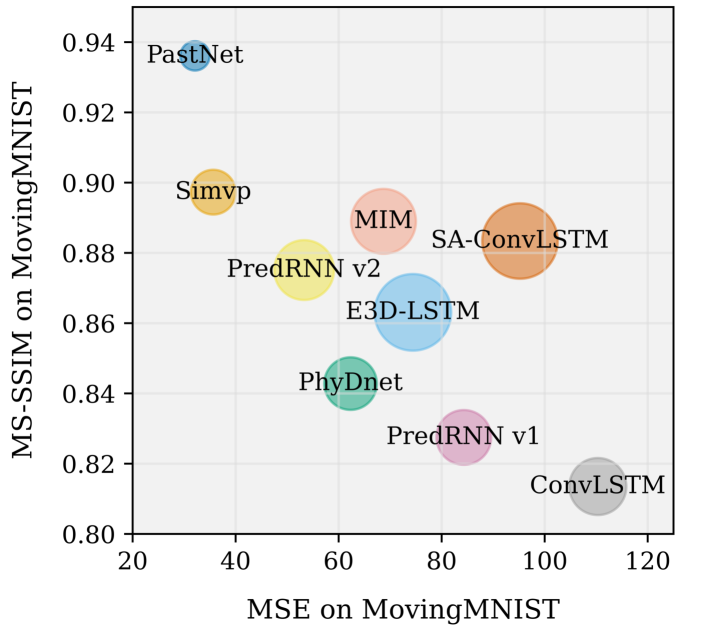
To address these concerns, this paper introduces a novel approach called Physics-assisted Spatio-temporal Network (PastNet) for high-quality video prediction. The croe of our PastNet is to introduce inductive physical bias using the data itself, which holds the potential to solve underlying PDEs. Specifically, we introduce a convolution operator in the spectral space that initially transfers video frames into the Fourier domain, followed by efficient parallelizable channel fusion (Guibas et al., 2021a). Subsequently, we employ an inverse Fourier transform to generate the outputs. Furthermore, to enhance efficiency for high-resolution video implementation, our PastNet introduces a discrete spatio-temporal module, which not only estimates intrinsic dimensionality but also introduces memory banks to discretize local features during the processing of complex spatio-temporal signals, replacing local features with their nearest queries from the memory bank. Finally, a deconvolution decoder is incorporated to output the predictions, which are combined with outputs from the spectral space. Comprehensive experiments on various benchmark datasets substantiate the effectiveness and efficiency of our proposed PastNet. A glimpse of the compared results by various approaches is provided in Figure 1 and we can observe the huge superiority of our PastNet on MovingMNIST. Our main contributions can be summarized as follows:

• New Perspective. We open up a new perspective to connect spatio-temporal video prediction with physical inductive biases, thereby enhancing the model with data itself.

• Novel Methodology. Our PastNet not only employs a convolution operator in the spectral space to incorporate physical prior but also discretizes local features using a memory bank with the estimated intrinsic dimensionality to boost efficiency for high-resolution video prediction.

• High Performance and Efficiency. Comprehensive experiments on a variety of datasets demonstrate that the PastNet exhibits competitive performance in terms of both effectiveness and efficiency.

2. Related Work

2.1. Spatio-temporal Video Prediction

Video prediction has emerged as an essential topic within the multimedia research community, and numerous methods have been proposed to address this challenge. Initial studies frequently examine spatio-temporal signals extracted from RGB frames (Shi et al., 2015; Lotter et al., 2017; Villegas et al., 2017; Wu et al., 2022; Wang et al., 2022). For instance, ConvLSTM (Shi et al., 2015) employs convolutional neural networks (CNNs) to encode spatial data, which is subsequently integrated with an LSTM model to capture temporal dependencies. PredNet (Lotter et al., 2017) draws inspiration from neuroscience, enabling each layer to make local predictions for video sequences. MCnet (Villegas et al., 2017) introduces multiple pathways to encode motion and content independently, which are combined into an end-to-end framework. Various approaches strive to merge video prediction with external information from optical flow, semantic maps and human posture data (Liu et al., 2017; Lee et al., 2021; Wang et al., 2018; Pan et al., 2019). As a representative unsupervised method, DVF (Liu et al., 2017) predicts missing frames using masked ones. HVP (Lee et al., 2021) treats this problem as video-to-video translation from semantic structures, inspired by hierarchical models. SADM (Bei et al., 2021) combines semantic maps and flow fields to provide more compatible contextual information. However, this external information could be inaccessible in real-world applications (Pan et al., 2019; Wu et al., 2020; Hu et al., 2023a). Furthermore, the efficiency and effectiveness of current solutions remain suboptimal for high-resolution videos. To surmount these obstacles, we propose a novel method that incorporates both physical inductive biases and quantization operations for high-quality video prediction.

2.2. Physics-Informed Machine Learning

Various machine learning problems can benefit from the incorporation of physical knowledge (Karniadakis et al., 2021). Modern physics-informed machine learning approaches can leverage knowledge from three aspects, i.e., observational biases, inductive biases, and learning biases. Observational biases primarily arise from the data itself (Lu et al., 2021; Li et al., 2020; Yang and Perdikaris, 2019), offering a range of data augmentation strategies to expand datasets. Inductive biases guide the specific design of neural networks such as graph neural networks (Bronstein et al., 2017) and equivariant networks (Cohen et al., 2019), which possess properties of respecting additional symmetry groups (Bronstein et al., 2017). Learning biases pertain to the process of imposing distinct constraints by incorporating loss objectives during optimization (Geneva and Zabaras, 2020), adhering to the principles of multi-task learning. For instance, physics-inspired neural networks (Raissi et al., 2019) (PINNs) typically include constraints related to derivatives from PDEs, resulting in superior performance in modeling dynamical systems and predicting molecular properties. To bolster predictive performance, our PastNet introduces inductive biases from the underlying PDEs of video frames by integrating learnable neural networks in the Fourier domain.

Figure 2. An overview of the proposed PastNet, which consists of a Fourier-based Physics-guided (FPG) and a Discrete Spatio-temporal (DST) module. The PFI module first divides video frames into non-overlapping patches and introduce Fourier-based spectral filter with the introduction of physical biases. Then, its also extract spatial signals with convolutional neural networks. The DST module is an encoder-decoder architecture, which introduces a memory bank to discretize local features in estimated intrinsic dimensionality.

2.3. Data Compression

Compressing large-scale data is essential for enhancing the efficiency of both training and inference processes (Morozov and Babenko, 2019). Learning to hash is a widely employed technique that accomplishes this by mapping continuous vectors to compact binary codes while preserving similarity relationships, which achieves extensive progress in approximate nearest neighbor search (Cao et al., 2017). Another line to address this challenge is neural quantization. For instance, multi-codebook quantization (Zhu et al., 2023) is akin to the process of k-means clustering, which stores centroids and assignments in the codebooks. Recently, VQ-VAE (Van Den Oord et al., 2017) has integrated neural quantization with auto-encoders, using discrete codes to reconstruct input images and leading to efficient models for large-scale applications. VQ-VAE has been successfully applied in various scenarios, including video generation (Yan et al., 2021), image inpainting (Peng et al., 2021), and semantic communication (Hu et al., 2023b). In this paper, our DST module is inspired by VQ-VAE, discretizing local features to improve efficiency in high-resolution video prediction.

3. Methodology

3.1. Overview

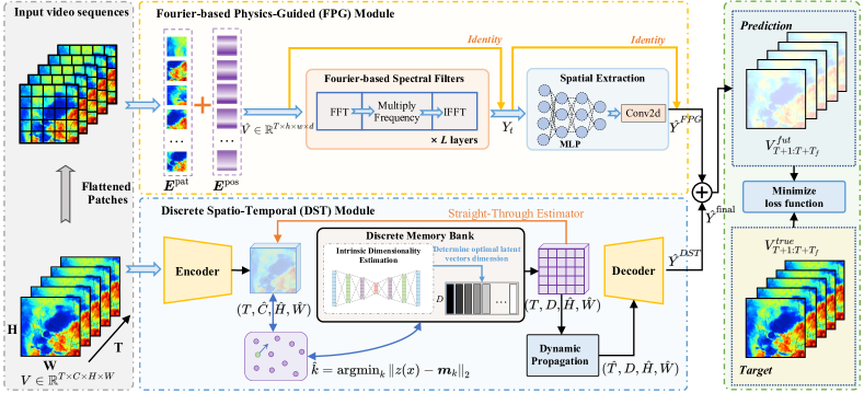
This paper studies the problem of spatio-temporal video prediction and existing solutions usually neglect underlying physical principles and suffer from larger computational space. To tackle this, our proposed PastNet introduces both Fourier-based physics-guided (FPG) module and discrete spatio-temporal (DST) module for effectively and efficiently video prediction as in Figure 2. In particular, our FPG module first divides frame into non-overlapping patches and then introduce a Fourier-based priori spectral filters with the introduction of physical inductive biases. Then, our DST module not only estimates intrinsic dimensionality but also introduces a discrete memory bank to effectively and efficiently capture spatio-temporal signals. Following is the problem definition and the detailed description of these key components of our proposed PastNet.

Problem Definition. To enhance clarity, we offer a comprehensive explanation of the relevant concepts. Assume a video trajectory represents a dynamic physical system in the temporal domain, consisting of $T$ time steps, denoted as $\bm{V}_{1:T}=\{\bm{V}_{1},\cdots,\bm{V}_{T}\}$. Each snapshot captures $C$ color space measurements over time at all locations within a spatial region, represented by an $H\times W$ grid. From a spatial viewpoint, the observation of these $C$ measurements at any specific time step $i$ can be depicted as a tensor, $\bm{V}_{i}\in\mathbb{R}^{C\times H\times W}$. Our objective is to leverage spatio-temporal data to deduce underlying physical priors and integrate feature representation learning in both spatial and temporal dimensions and predict the most probable future sequence of length $T_{f}$, denoted as ${\bm{V}}^{fut}_{T+1:T+T_{f}}=\{\bm{V}_{T+1},\cdots,\bm{V}_{T+T_{f}}\}$.

3.2. Fourier-based Physics-Guided (FPG) Module

Our primary insight focuses on utilizing prior physical signals to achieve effective spatio-temporal video prediction. In fact, spatio-temporal data is often subject to complex, high-dimensional nonlinear physical equations (e.g., Navier-Stokes equation), which are challenging to capture. Inspired by previous studies (Li et al., 2020; Guibas et al., 2021a), we employ spectral methods and develop an algorithm that seamlessly combines trainable neural networks with Fourier-based a priori spectral filters. It has been shown that the features transformed through Fourier transformation in the frequency domain correspond precisely with the coefficients of the underlying physical partial differential equation (Li et al., 2020; Guibas et al., 2021b). As a result, we can utilize neural networks to approximate the analytical solution of the latent PDE. To be specific, we initially divide video frames into non-overlapping patches with initialized embeddings and subsequently transform them into a spectral space. The features within the frequency domain are fused, followed by an inverse transformation returning them to the spatial domain. This innovation supports a physical inductive bias derived from data, demonstrating significant potential for solving PDEs. Then, we introduce our FPG module in detail.

Embedding Initialization. Given the input video $\bm{V}\in\mathbb{R}^{T\times C\times H\times W}$, we extract the high-level learnable representations following ViT (Dosovitskiy et al., 2020). In particular, we divide the frame into non-overlapping $N=HW/hw$ patches of size $h\times w$ and then project them into patch embeddings $\bm{E}^{pat}\in\mathbb{R}^{T\times h\times w\times d}$, where $d$ denotes the embedding dimension. Position embeddings $\bm{E}^{pos}\in\mathbb{R}^{h\times w\times d}$ are also applied to get the initial token representation matrix $\hat{\bm{V}}\in\mathbb{R}^{T\times h\times w\times d}$. In formulation,

(1) $$\hat{\bm{V}}_{t}=\bm{E}^{pat}_{t}+\bm{E}^{pos},$$

where $\hat{\bm{V}}_{t}=\hat{\bm{V}}[t,:,:]\in\mathbb{R}^{h\times w\times d}$ makes up the matrix $\hat{\bm{V}}$.

Fourier-based Spectral Filter. We apply $\hat{\bm{V}}$ as input to $L$ layers of filters, each layer containing three essential components, i.e., Fourier transform, separate mixing and inverse Fourier transform. Firstly, a 2D fast Fourier transform (FFT) is leveraged to generate the frequency domain token $\mathcal{K}_{t}\in\mathbb{R}^{h\times w\times d}$ at time step $t$:

(2) $$\mathcal{K}_{t}(u,v)=\sum_{x=0}^{h-1}\sum_{y=0}^{w-1}\hat{\bm{V}}_{t}(x,y)e^{-2\pi i(\frac{u}{h}x+\frac{v}{w}y)},$$

where $i$ is the imaginary unit, and $u$ and $v$ are the indices of rows and columns in the frequency domain, respectively.

Secondly, the complex-valued token $\mathcal{K}=\mathcal{K}_{1:T}$ is then split into its real and imaginary parts and concatenated along the channel dimension. To enhance the integration of feature information, we utilize token mixing across different channels, which allows for richer Fourier mode representations to emerge through greater fusion of channel-wise signals. It is implemented with separate MLPs for the real and imaginary parts separately as follows:

(3) $$\Re\mathcal{\hat{K}}_{t}(u,v)=\operatorname{MLP}_{\theta_{1}}(\Re\mathcal{K}_{t}(u,v)),\Im\mathcal{\hat{K}}_{t}(u,v)=\operatorname{MLP}_{\theta_{2}}(\Im\mathcal{K}_{t}(u,v)),$$

where $\Re$ and $\Im$ denotes the operator to obtain the real part and imaginary part, respectively. Performing token mixing mixes different modes across the Fourier domain. As the Fourier domain possesses global attributes, it further explore long-range relationships for underlying physical features.

Lastly, the mixed tokens are then transformed back to the spatial domain using the 2D inverse Fourier transform to obtain the output of spectral filter layers $\bm{Y}\in\mathbb{R}^{T\times h\times w\times d}$ as follows:

(4) $$\begin{split}\bm{Y}_{t}(x,y)&=\frac{1}{hw}\sum_{u=0}^{h-1}\sum_{v=0}^{\frac{w}{2}}\mathcal{\hat{K}}_{t}(u,v)e^{2\pi i(\frac{u}{h}x+\frac{v}{w}y)}\\ &+\frac{1}{hw}\sum_{u=0}^{h-1}\sum_{v=\frac{w}{2}+1}^{w-1}\mathcal{\hat{K}}_{t}(u,v)e^{2\pi i(\frac{u}{h}x+\frac{v-w}{w}y)},\end{split}$$

where ${\bm{Y}}_{t}={\bm{Y}}[t,:,:]\in\mathbb{R}^{N\times M}$ makes up the matrix $\bm{Y}$.

Spatial Extraction. To better extract the latent spatial information, we introduce classic convolutional neural networks as a supplement of the priori spectral filters, which can be formulated as follows:

(5) $${\bm{\hat{Y}}}^{FPG}_{t}=\operatorname{Tanh}(\operatorname{Conv2d}(\operatorname{MLP}(\bm{Y}_{t})+\bm{Y}_{t})),$$

The convolutional layer is known for its ability to extract features in the spatial domain through its local receptive fields. By leveraging these learned features as filters in the frequency domain, the convolutional layer can effectively mine potential physical information from the input data. The extracted physical information can significantly enhance the performance of spatiotemporal prediction.

Overall, the Fourier-based physics-guided module transforms the spatial domain of latent physical information into the frequency domain using Fourier transforms, and learns the analytical solutions of PDEs using neural networks. This approach allows PastNet to handle complex geometries and high-dimensional problems.

3.3. Discrete Spatio-temporal (DST) Module

Our discrete spatio-temporal (DST) module aims to explore spatio-temporal signals in video frames in an efficient manner. To achieve this, we not only estimate the intrinsic dimensionality for the hidden space, but also introduces a memory bank to vector quantization. In particular, it consists of four different modules, i.e., encoder, intrinsic dimensionality estimation, discrete quantization, dynamic propagation and decoder. Then, we introduce them in detail.

Encoder. The encoder contains $K_{e}$ ConvNormReLU blocks to capture spatial signals. Given $\bm{Z}^{(0)}=\bm{V}$ and an activation function $\sigma$, we have:

(6) $$\bm{Z}^{(i)}=\sigma\left(\operatorname{LayerNorm}\left(\operatorname{Conv2d}\left(\bm{Z}^{(i-1)}\right)\right)\right),1\leq i\leq K_{e},$$

where $\bm{Z}^{(i-1)}$ and $\bm{Z}^{(i)}$ denote the input and output of the $i$-th block with the shapes $(T,C,H,W)$ and $(T,\hat{C},\hat{H},\hat{W})$, respectively.

Intrinsic Dimensionality Estimation. How to decide the dimensionality of the hidden space remains a challenging problem (Chen et al., 2022). In particular, too large dimensionality would bring in redundant computational time and potential overfitting while too small one would underfit data. Here, we turn to Levina–Bickel algorithm (Levina and Bickel, 2004) to acquire intrinsic dimensionality.

In particular, we start with a large dimensionality followed by mapping $\bm{Z}^{(K_{e})}$ back to the input using a decoder and minimize the reconstruction loss objective as $L_{rec}=||\bm{V}-\hat{\bm{V}}||$ where $\hat{\bm{V}}$ is the reconstructed frame. Then, we identify the $R$ nearest neighbours for each vector $\bm{h}_{j}\in\bm{Z}^{(K_{e})}$, i.e., $\{\bm{h}_{j_{1}},\cdots,\bm{h}_{j_{R}}\}$ and calculate the local estimator for the vector as:

(7) $$D_{j}=\frac{1}{R-2}\sum_{m=1}^{R-1}\log\frac{d(\bm{h}_{j},\bm{h}_{j_{R}})}{d(\bm{h}_{j},\bm{h}_{j_{m}})},$$

where $d(\cdot,\cdot)$ denotes the cosine distance between two vectors. Finally, we take the average all local estimators to generate the final estimator:

(8) $$D=\frac{1}{J}\sum_{j=1}^{J}D_{j},$$

where $J$ is the number of vectors in $\bm{Z}^{(K_{e})}$ and $\cdot$ denotes the ceiling function. After generating final estimated optimal dimension, we utilize $D$ as the hidden embedding instead.

Discrete Quantization. Previous methods usually process video features directly using spatio-temporal convolution modules. However, directly feeding video features into these modules would bring in huge computational cost. Therefore, we introduce a discrete memory bank to discretize feature vectors, which are constructed by an variational autoencoder (Van Den Oord et al., 2017; Yan et al., 2021). In this way, computational costs can be largely reduced to fit for large-scale video prediction.

In detail, we initialize the memory bank with variational autoencoder. Here, each embedding vector $\bm{z}$ from $\bm{Z}^{(K_{e})}$ from the output of the encoder is mapped to the nearest point in the memory bank. The number of embeddings in the memory is set to $D^{2}$ empircally. Given the memory bank with $D^{2}$ embedding vectors, $\{\bm{m}_{1},\cdots,\bm{m}_{D^{2}}\}$, we construct a mapping $VQ$:

(9) $$VQ(\bm{z})=\bm{m}_{\hat{k}},\quad\text{ where }\quad\hat{k}=\operatorname{argmin}_{k}\left\|\bm{z}(\bm{x})-\bm{m}_{k}\right\|_{2},$$

where each embedding $\bm{z}$ is concatenated to generate matrix $\bar{Z}=VQ(\bm{Z}^{(K_{e})})$. The mapping connects continuous vectors with given vectors in the memory bank to save the computational cost. Then, to minimize the information loss, we map the concatenated matrix back to the input using a new decoder, i.e., $\tilde{\bm{V}}=Dec(\bar{Z})$. The whole framework is optimized using the following objective as:

(10) $$\mathcal{L}=||\bm{V}-\tilde{\bm{V}}||+\left\|\operatorname{sg}\left[\bar{Z}\right]-\bm{Z}^{(K_{e})}\right\|_{2}^{2}+\beta\left\|\bar{Z}-\operatorname{sg}[\bm{Z}^{(K_{e})}]\right\|_{2}^{2},$$

where $\beta$ denotes a parameter to balance these objective and $\operatorname{sg}(\cdot)$ is the stopgradient operator to cut off the gradient computation during back propagation. Here, the first term denotes the reconstruction loss and the last two terms minimize the quantization loss between continuous embedding vectors and their neighbours in the memory bank.

Dynamic Propagation. After training the variational autoencoder, we remove the decoder, and then feed the quantized vector into temporal convolution on $T\times D$ channels. In particular, each temporal convolution block involves a bottleneck followed by group convolution operator:

(11) $$\bm{Z}^{(i)}=\operatorname{GroupConv2d}(\operatorname{Bottleneck}(\bm{Z}^{(i-1)})),K_{e}<i\leq K_{e}+K_{t},$$

where $\operatorname{Bottleneck}$ denotes the 2D convolutional layer with $1\times 1$ kernel and $K_{t}$ is the number of blocks. The shape of input $\bm{Z}^{(i-1)}$ and output $\bm{Z}^{(i)}$ are $(T,D,\hat{H},\hat{W})$ and $(\hat{T},D,\hat{H},\hat{W})$, respectively.

Decoder. Finally, our decoder contains $K_{d}$ unConvNormReLU blocks to output the final predictions $\hat{\bm{Y}}^{DST}=\bm{Z}^{(K_{e}+K_{t}+K_{d})}$. In formulation, we have:

(12) $$Z^{(i)}= \sigma\left(\operatorname{LayerNorm}\left(\operatorname{unConv2d}\left(Z^{(i-1)}\right)\right)\right),$$

$$K_{e}+K_{t}+1\leq i\leq K_{e}+K_{t}+K_{d},$$

where $\operatorname{unConv2d}$ is implemented using ConvTranspose2d (Dumoulin and Visin, 2016). The shape of input $\bm{Z}^{(i-1)}$ and output $\bm{Z}^{(i)}$ are $(\hat{T},D,\hat{H},\hat{W})$ and $(T,C,H,W)$, respectively.

3.4. Framework Summarization

Finally, we combine the output of both FPG and DST modules, which result in the final prediction:

(13) $$\hat{\bm{Y}}^{final}=\hat{\bm{Y}}^{FPG}\oplus\hat{\bm{Y}}^{DST},$$

where $\oplus$ represents element-wise addition. The whole framework would be optimizing by minimizing the vanilla MSE loss between the predictions and the target frame.

4. Experiment

4.1. Experimental Setups

Datasets. In this paper, the datasets studied can be classified into two categories from the perspective of PDE modeling or physics equation description: Non-natural Phenomenon datasets and Natural Phenomenon datasets. The former includes MovingMNIST (Srivastava et al., 2015), TrafficBJ (Zhang et al., 2017), and KTH datasets (Schuldt et al., 2004). Although they do not correspond to natural phenomena, the dynamic evolutionary processes expressed in these datasets can still be described by PDEs. The latter includes the Storm EVent ImagRy (SEVIR) (Veillette et al., 2020), Reaction Diffusion System (RDS), Elastic Double Pendulum System (EDPS), and Fire System (FS) datasets (Chen et al., 2022), which correspond to natural phenomena such as meteorology, chemical reactions, mechanical vibrations, and fire. These datasets are often used in the study of PDE modeling and the description of physics equations to better understand and predict the evolution of natural phenomena. We conduct experiments on seven datasets for evaluation. Here we summarize the details of the datasets used in this paper, The statistics are shown in the Table 1.

Table 1. Statistics of the datasets used in the experiments. The number of training and test sets of the dataset are $N\_train$ and $N\_test$ respectively, where the size of each image frame is ($C,H,W$), and the length of the input and prediction sequences are $T$, $K$ respectively.

Dataset	$N\_train$	$N\_test$	($C,H,W$)	$T$	$K$
MovingMNIST	9000	1000	(1, 64, 64)	10	10
TrafficBJ	19627	1334	(2, 32, 32)	4	4
KTH	108717	4086	(1, 128, 128)	10	20
SEVIR	4158	500	(1, 384, 384)	10	10
RDS	2000	500	(3, 128, 128)	2	2
EDPS	2000	500	(3, 128, 128)	2	2
FS	2000	500	(3, 128, 128)	2	2

Evaluation metrics. We adopt Mean Squared Error (MSE), Mean Absolute Error (MAE), Multi-Scale Structural Similarity (MS-SSIM), Peak Signal-to-Noise Ratio (PSNR), and Learned Perceptual Image Patch Similarity (LPIPS) to evaluate the quality of the predictions. Lower values of MSE, MAE, and LPIPS and higher values of SSIM and PSNR imply better performance.

Implementation details. The PastNet model features a consistent backbone architecture for all datasets, in which the FPG component is composed of 8-$layer$ Fourier-based Spectral Filter. The DSM encoder incorporates 3-$layer$ convolution block layers and 3-$layer$ residual blocks, while the decoder utilizes 1-$layer$ convolution block, 4-$layer$ residual blocks, and 2-$layer$ deconvolution blocks. All experiments in this paper were conducted on an NVIDIA A100-PCIE-40GB.

4.2. Performance Comparison

Table 2. Quantitative prediction results of PastNet compared to Baselines on various Non-natural Phenomenon datasets. The evaluation metrics selected for this study are MSE $\downarrow$, MAE $\downarrow$, MS-SSIM $\uparrow$, and PSNR $\uparrow$, with a lower value ($\downarrow$) indicating better performance for MSE and MAE, and a higher value ($\uparrow$) indicating better performance for MS-SSIM and PSNR. The best result is indicated in boldface, while the second-best result is indicated with an underline in the table caption.

Method	MovingMNIST				TrafficBJ				KTH
	MSE	MAE	MS-SSIM	PSNR	MSE x 100	MAE	MS-SSIM	PSNR	MSE	MAE / 10	MS-SSIM	PSNR
ConvLSTM	105.41	188.96	0.7498	26.27	48.45	18.921	0.9782	37.72	126.15	128.32	0.7123	23.58
PredRNN-V1	81.87	147.31	0.8697	29.99	46.49	17.784	0.9789	38.11	101.52	99.21	0.8292	25.55
E3D LSTM	67.25	136.99	0.8907	31.02	44.89	17.219	0.9731	38.71	86.17	85.55	0.8663	27.92
SA-ConvLSTM	79.76	142.21	0.8692	30.21	43.99	17.093	0.9672	38.98	89.35	87.20	0.8372	27.25
PhyDnet	58.22	145.76	0.9012	32.13	42.21	16.975	0.9821	39.94	66.95	56.73	0.8831	28.02
MIM	66.28	119.87	0.9017	31.12	43.98	16.645	0.9712	38.99	56.59	54.86	0.8666	28.97
PredRNN-V2	48.42	126.18	0.8912	33.19	43.89	16.982	0.9723	39.02	51.15	50.64	0.8919	29.92
SimVP	32.22	90.12	0.9371	37.17	43.32	16.897	0.9822	39.29	40.99	43.39	0.9061	33.72
PastNet	31.77	89.33	0.9447	38.38	42.93	16.405	0.9876	39.42	33.83	35.26	0.9279	35.28

Table 3. Quantitative prediction results of PastNet compared to Baselines on various Natural Phenomenon datasets. The evaluation metrics selected for this study are MSE $\downarrow$, MAE $\downarrow$, MS-SSIM $\uparrow$, and PSNR $\uparrow$, with a lower value ($\downarrow$) indicating better performance for MSE and MAE, and a higher value ($\uparrow$) indicating better performance for MS-SSIM and PSNR. The best result is indicated in boldface, while the second-best result is indicated with an underline in the table caption.

Dataset	Model	MSE	MAE	MS-SSIM	PSNR
	DLP	300.42	140.82	0.6772	36.59
	PhyDnet	97.70	72.22	0.7137	43.03
SEVIR	NLDM	295.93	170.73	0.6982	36.71
	SimVP	68.68	47.71	0.7231	49.09
	PastNet	66.13	44.84	0.7568	49.78
	DLP	1.38	2.08	0.9763	44.52
	PhyDnet	0.51	1.25	0.9874	47.01
RDS	NLDM	1.03	1.78	0.9594	46.56
	SimVP	0.15	0.67	0.9896	51.06
	PastNet	0.13	0.63	0.9997	51.79
	DLP	3.53	281.82	0.9337	42.53
	PhyDnet	1.08	167.23	0.9983	45.92
EDPS	NLDM	2.51	237.43	0.9455	42.83
	SimVP	0.93	150.11	0.9882	46.25
	PastNet	0.94	168.53	0.9991	45.98
	DLP	7.78	426.12	0.9266	38.38
	PhyDnet	4.41	327.32	0.9423	40.47
FS	NLDM	7.21	411.14	0.9392	38.62
	SimVP	3.01	261.19	0.9647	42.03
	PastNet	2.19	222.08	0.9861	43.24

Figure 3. Example of prediction results for the Moving MNIST dataset. Top: input motion digital sequence; Middle: future real motion digital sequence; Bottom: PastNet predicted motion digital sequence.

Figure 4. Example of prediction results on the TrafficBJ dataset. Top: input Traffic flow; Middle: future real Traffic flow; Bottom: PastNet predicted Traffic flow.

Table 4. Experimental results of ablation with different model structures on the SEVIR dataset.The evaluation metrics selected for this study are MSE $\downarrow$, MAE $\downarrow$, MS-SSIM $\uparrow$, and Time(h) $\uparrow$, with a lower value ($\downarrow$) indicating better performance for MSE, MAE and Time(h), and a higher value ($\uparrow$) indicating better performance for MS-SSIM.

Model	MSE	MAE	SSIM	Time (h)
PastNet w/o FPG	133.8	103.6	0.67	3.19
PastNet w/o FPG + UNet	115.4	99.35	0.61	16.54
PastNet w/o FPG + ViT	287.3	139.5	0.49	23.87
PastNet w/o FPG + SwinT	321.8	158.7	0.54	24.12
PastNet w/o DST	192.3	118.5	0.64	4.92
PastNet	73.21	52.31	0.74	4.16

Figure 5. Example of prediction results on the SEVIR dataset. Top: input weather sequence; Middle: future real weather sequence; Bottom: PastNet predicted weather sequence.

Figure 6. Inputs: The input weather sequences; Targets: Thefuture real weather sequences; I: PastNet predicts the weather sequences; II: PastNet w/o FPG predicts the weather sequences; III: PastNet w/o FPG + UNet predicts the weather sequences; IV: PastNet w/o FPG + ViT predicts the weather sequences; V: PastNet w/o FPG + SwinT predicts the weather sequences; VI: PastNet w/o DST predicts the weather sequences.

Figure 7. PastNet outperforms other models in terms of efficiency and convergence rate on the MovingMNIST dataset. Specifically, it achieves the lowest LPIPS score in the shortest training time, as shown on the Left side of the figure. In addition, it achieves the highest MS-SSIM and PSNR scores within the same epochs, as depicted in the Middle and Right sides of the figure, respectively.

Table 5. Performance metrics for solving PDE equations using PastNet. The table shows the mean squared error (MSE), mean absolute error (MAE), and time per epoch (in seconds) for the Navier-Stokes equations (NSE) and Shallow-Water equations (SWE) in their 2D forms.

PDE	Evaluation Criterion
	MSE	MAE	Time per epoch (s)
NSE	0.3021	28.4952	218
SWE	0.0185	8.0391	223

Figure 8. (a) presents qualitative visualization results for NSE, while (b) displays the qualitative visualization results for SWE. The examples of the input PDE equations flow are denoted by $I$, examples of future PDE equations are denoted by $II$, predicted PDE equation examples are denoted by $III$, and the error between predicted and true results is denoted by $IV$, which is measured using the relative L2 error metric. Specifically, the relative L2 errors are calculated to be 0.0072 and 0.0007 for NSE and SWE, respectively. The formula for calculating the relative L2 error is given by ${\rm Relative}\ L2\ {\rm Error}=\frac{\|\mathbf{y}-\hat{\mathbf{y}}\|_{2}}{\|\mathbf{y}-\bar{\mathbf{y}}\|_{2}}$, where $\mathbf{y}$ represents the true values, $\hat{\mathbf{y}}$ represents the predicted values, $\bar{\mathbf{y}}$ represents the mean of the true values, and $\|\cdot\|_{2}$ denotes the L2 norm. These results suggest that the model is able to make accurate predictions, with a particularly low relative L2 error for SWE.

We conduct a thorough evaluation of PastNet by comparing it with several baseline models on both non-natural and natural phenomena datasets. This includes competitive RNN architectures such as ConvLSTM (Shi et al., 2015), PredRNN-V1-2 (Wang et al., 2022), E3D LSTM (Wang et al., 2019a), SA-ConvLSTM (Lin et al., 2020), PhyDnet (Guen and Thome, 2020), and MIM (Wang et al., 2019b). We also evaluate state-of-the-art CNN architecture SimVP (Gao et al., 2022) for non-natural phenomena datasets. For natural phenomenon datasets, we evaluate models that incorporate physical information, such as DLP (de Bezenac et al., [n.d.]), which uses an advection-diffusion flow model and achieves state-of-the-art performance on the SST dataset, it is commonly used for generic physical processes. We also evaluate NLDM (Chen et al., 2022), which combines manifold learning theory and autoencoder to discover fundamental variables hidden in physical experimental data for spatiotemporal prediction, as well as PhyDnet and SimVP. Our evaluation is meticulous to ensure the validity of the results.

Table 2 demonstrates that PastNet outperforms other models on non-natural phenomena datasets. Specifically, PastNet achieves the best MSE and MAE metrics on MovingMNIST, with values that are 20% and 10% lower than SimVP, respectively. Moreover, PastNet also achieves higher MS-SSIM and PSNR metrics than other models, indicating better prediction ability for dynamic changes in videos. On TrafficBJ, while PhyDnet has the best MSE and PSNR performance, PastNet comes in second place and achieves top spot for MAE and MS-SSIM. On KTH, PastNet achieves the best MSE and MAE performance, with values that are 33.6% and 35.8% lower than the second-place MIM model, respectively. Overall, PastNet shows significant advantages over other baseline methods in all evaluation metrics.

Results in Table 3 show that PastNet achieves the best performance in most evaluation metrics for all natural phenomena datasets. On the SEVIR dataset, PastNet achieves the lowest MSE and MAE scores, significantly better than other methods such as DLP, PhyDnet, and NLDM. On the RDS dataset, PastNet achieves the lowest MSE x 100 score, significantly better than other methods. On the EDPS dataset, PastNet achieves the highest MS-SSIM score, significantly better than SimVP. Overall, these results demonstrate that PastNet is highly effective in accurately predicting physical quantities and preserving structural information in various physical datasets, outperforming other state-of-the-art methods such as DLP, PhyDnet, NLDM, and SimVP.

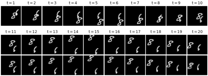
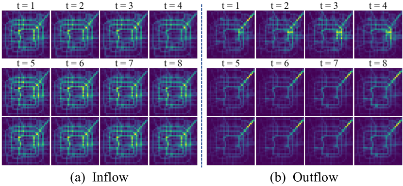
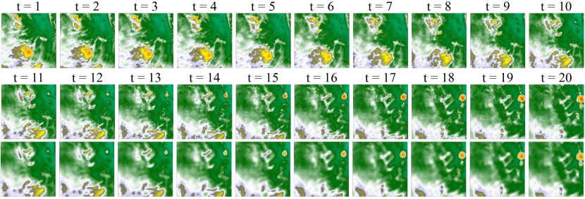
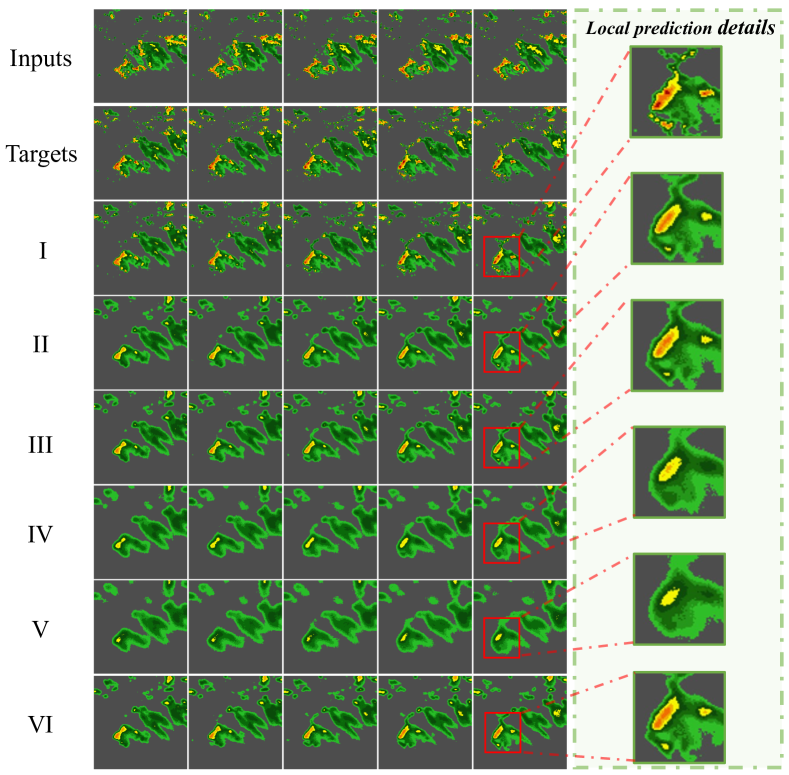
We present the qualitative prediction results of PastNet for various datasets, highlighting its capability to accurately predict future images. Our findings demonstrate that PastNet can accurately predict numerical motions in MovingMNIST as depicted in Figure 3. Additionally, Figure 4 shows that PastNet reliably predicts traffic flow changes in the TrafficBJ dataset. Furthermore, PastNet performs well in the SEVIR weather dataset, as shown in Figure 5, where it accurately predicts high-resolution satellite images and infers future weather changes. The visualization results for other datasets are available in the Appendix A.

4.3. Ablation Study

In this section, we demonstrate PastNet’s competitive performance on a wide range of datasets through a series of ablation studies. Table 4 and Figure 6 present the quantitative and qualitative results of these studies for different model structures, respectively. Specifically, PastNet w/o FPG removes the FPG module from the PastNet model. PastNet w/o FPG + UNet removes the FPG module from the PastNet model and uses UNet as an alternative module. PastNet w/o FPG + ViT removes the FPG module from the PastNet model and uses ViT as an alternative module. PastNet w/o FPG + SwinT removes the FPG module from the PastNet model and uses SwinT as an alternative module. PastNet w/o DST removes the DST module from the PastNet model. PastNet is the base PastNet model, which includes both the DST and FPG modules.

• PastNet outperforms other models with the lowest MSE, MAE, and highest SSIM, indicating its superior performance in video prediction.

• The inclusion of the DST module in PastNet improves the model’s training speed, making it a more efficient option.

• The FPG module is crucial for improving PastNet’s performance on the Natural Phenomenon dataset, with Unet as a potential alternative. This demonstrates PastNet’s versatility and ability to adapt to different datasets and tasks.

4.4. Efficiency and Convergence Rate Analysis

Figure 7 on the left side clearly demonstrates the advantages of PastNet in terms of both time and LPIPS metrics. Notably, PastNet’s training time for 100 epochs is only 4.16 hours, considerably faster than other models. Additionally, it achieves outstanding results in terms of LPIPS scores, indicating that PastNet can complete training more efficiently in a shorter amount of time while generating higher-quality images. The middle and right sides of Figure 7 illustrate the rapid improvement of PastNet in SSIM and PSNR metrics. Within approximately 60 epochs, PastNet achieves an SSIM metric of around 0.92, while other models remain below 0.85 at the same point. After 100 epochs, PastNet reaches a PSNR metric of approximately 38, which is far superior to other models. These results highlight PastNet’s superior convergence rate during training, enabling it to rapidly produce high-quality image results. In summary, PastNet is an accurate and efficient model for video prediction, with fast convergence and high-quality results. It represents a promising direction for future research and practical applications.

4.5. Potential for Solving PDE Equations

To investigate the potential of PastNet for solving physical problems, we consider the Navier-Stokes equations, which represent viscous incompressible fluids in the form of vorticity on the unit torus, and the Shallow-Water equations, which are obtained from the general Navier-Stokes equations. We focus on their 2D forms, and more detailed descriptions of them are shown in Appendix B.

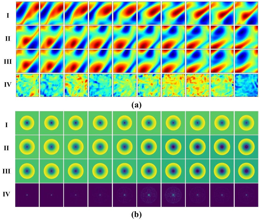
We use PastNet to solve the Navier-Stokes equations with viscosity $\nu=10^{-3}$ and a resolution of 64 $\times$ 64 for training and testing. We use the flow field at 10 input time steps to predict the flow field at 10 future time steps ($10_{timesteps}\mapsto 10_{timesteps}$). For the Shallow-Water equations, we fix the resolution to 128 $\times$ 128 for training and testing and use the flow field at 50 input time steps to predict the flow field at 50 future time steps ($50_{timesteps}\mapsto 50_{timesteps}$). We train for 200 epochs and record the metrics MSE, MAE, and the time per epoch. The quantitative and qualitative results are presented in Table 5 and Figure 8, respectively.

The results in Table 5 indicate that PastNet has potential for solving PDE equations, especially for the SWE equation, as it achieved lower MSE and MAE values for the SWE equation than for the NSE equation, while the time per epoch was similar for both equations.

5. Conclusion

In this paper, we investigate the problem of spatio-temporal video prediction and propose a novel method named PastNet to tackle the problem. The key insight of our PastNet is to incorporate a spectral convolution operator in the Fourier domain, which effectively introduces inductive biases from the underlying physical laws. Moreover, we introduce both local feature discretization and intrinsic dimensionality estimation to reduce the computational costs with accuracy retained. Extensive experiments on a range of popular datasets show that the proposed PastNet is more effective and efficient than state-of-the-art techniques. In future works, we would develop more effective video prediction techniques by introducing high-level physical domain knowledge in various fields.

APPENDIX

Appendix A Visual presentation of prediction results

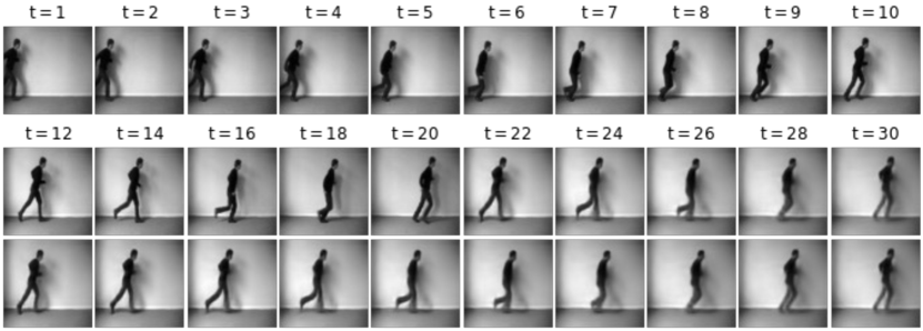
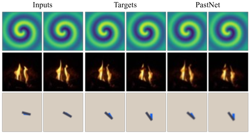
The visualization results for the other datasets are shown below: Figure9 demonstrates PastNet’s proficiency in the KTH pedestrian motion dataset, accurately predicting future pedestrian trajectories; Finally, Figure10 illustrates PastNet’s capability in predicting the systematic evolution of physical dynamics datasets such as RDS, EDPS, and FS.

Figure 9. Example of prediction results on the KTH dataset. Top: input Pedestrian movement sequence; Middle: future real Pedestrian movement sequence; Bottom: PastNet predicted Pedestrian movement sequence.

Figure 10. Examples of prediction results on the Reaction Diffusion System, Elastic Double Pendulum System and Fire System datasets; two input frames predict two output frames; from left to right, the input sequence, the target sequence and the PastNet prediction sequence.

Appendix B Description of the details of the PDE equations

B.1. 2D Navier-Stokes Equations

This paper considers the 2D Navier-Stokes equations for a viscous, incompressible fluid with vorticity in the form of a curl on the unit torus.

(14) $$\partial_{t}w(x,t)+u(x,t)\cdot\nabla w(x,t) =\nu\Delta w(x,t)+f(x) x\in(0,1)^{2},t\in(0,T]$$

$$\nabla\cdot u(x,t) =0, x\in(0,1)^{2},t\in[0,T]$$

$$w(x,0) =w_{0}(x), x\in(0,1)^{2}$$

In this context, $u\in C([0,T];H_{r}^{per}((0,1)^{2};\mathbb{R}^{2}))$ for any $r>0$ is the velocity field, $w=\nabla\times u$ is the vorticity, $w_{0}\in L^{2}_{per}per((0,1)^{2};\mathbb{R})$ is the initial vorticity, $\nu\in\mathbb{R}^{+}$ is the viscosity coefficient, and $f\in L^{2}_{per}((0,1)^{2};\mathbb{R})$ is the forcing function. The time evolution of the equation is visualized in Figure 11.

Figure 11. This visualization concerns the time evolution of data generated by the 2D Navier-Stokes equations.

B.2. 2D Shallow-Water Equations

The Navier-Stokes equations are the fundamental equations that describe viscous flow in fluid mechanics. The shallow water equations can be derived from the Navier-Stokes equations and are used to model free-surface flow problems. In two dimensions, these equations can be expressed as a system of hyperbolic partial differential equations.

Figure 12. This visualization concerns the time evolution of data generated by the 2D shallow water equations.

(15) $$\partial_{t}h+\partial_{x}hu+\partial_{y}hv = 0$$

(16) $$\partial_{t}hu+\partial_{x}\left(u^{2}h+\frac{1}{2}g_{r}h^{2}\right) = -g_{r}h\partial_{x}b$$

(17) $$\partial_{t}hv+\partial_{y}\left(v^{2}h+\frac{1}{2}g_{r}h^{2}\right) = -g_{r}h\partial_{y}b$$

In the shallow water equations, which are used to model free-surface flow problems, $u$ and $v$ represent the horizontal and vertical velocities, $h$ represents the water depth, and $b$ describes the spatial variation of the depth. The terms $hu$ and $hv$ can be interpreted as the directional momentum components, and $g$ represents the acceleration due to gravity.

The benchmark for the shallow water equation problem presented in Subsection 4.5 includes a specific simulation of a two-dimensional radial dam-breaking scheme. The simulation takes place on a square domain $\Omega=[-2.5,2.5]^{2}$, where the initial water height is represented by a circular bulge at the center of the domain.

(20) $$h(t =0,x,y)=\left\{\begin{array}[]{ll}2.0,&\text{ for }r<\sqrt{x^{2}+y^{2}}\\ 1.0,&\text{ for }r\geq\sqrt{x^{2}+y^{2}}\end{array}\right.$$

The time evolution of the equation is visualized in Figure 12.

References

- (1)
- Babaeizadeh et al. (2017) Mohammad Babaeizadeh, Chelsea Finn, Dumitru Erhan, Roy H Campbell, and Sergey Levine. 2017. Stochastic variational video prediction. In Proceedings of the International Conference on Learning Representations.
- Bei et al. (2021) Xinzhu Bei, Yanchao Yang, and Stefano Soatto. 2021. Learning semantic-aware dynamics for video prediction. In Proceedings of the IEEE/CVF Conference on Computer Vision and Pattern Recognition. 902–912.
- Bronstein et al. (2017) Michael M Bronstein, Joan Bruna, Yann LeCun, Arthur Szlam, and Pierre Vandergheynst. 2017. Geometric deep learning: going beyond euclidean data. IEEE Signal Processing Magazine 34, 4 (2017), 18–42.
- Cao et al. (2017) Zhangjie Cao, Mingsheng Long, Jianmin Wang, and Philip S Yu. 2017. Hashnet: Deep learning to hash by continuation. In Proceedings of the IEEE/CVF International Conference on Computer Vision. 5608–5617.
- Chang et al. (2022) Zheng Chang, Xinfeng Zhang, Shanshe Wang, Siwei Ma, and Wen Gao. 2022. Strpm: A spatiotemporal residual predictive model for high-resolution video prediction. In Proceedings of the IEEE/CVF Conference on Computer Vision and Pattern Recognition. 13946–13955.
- Chen et al. (2022) Boyuan Chen, Kuang Huang, Sunand Raghupathi, Ishaan Chandratreya, Qiang Du, and Hod Lipson. 2022. Automated discovery of fundamental variables hidden in experimental data. Nature Computational Science 2, 7 (2022), 433–442.
- Chen and Wang (2019) Xiongtao Chen and Wenmin Wang. 2019. Uni-and-bi-directional video prediction via learning object-centric transformation. IEEE Transactions on Multimedia 22, 6 (2019), 1591–1604.
- Cheng et al. (2019) Changmao Cheng, Chi Zhang, Yichen Wei, and Yu-Gang Jiang. 2019. Sparse temporal causal convolution for efficient action modeling. In Proceedings of the ACM International Conference on Multimedia. 592–600.
- Cohen et al. (2019) Taco Cohen, Maurice Weiler, Berkay Kicanaoglu, and Max Welling. 2019. Gauge equivariant convolutional networks and the icosahedral CNN. In Proceedings of the International Conference on Machine Learning. 1321–1330.
- de Bezenac et al. ([n.d.]) Emmanuel de Bezenac, Arthur Pajot, and Patrick Gallinari. [n.d.]. Deep Learning for Physical Processes: Incorporating Prior Scientific Knowledge. In International Conference on Learning Representations.
- Dosovitskiy et al. (2020) Alexey Dosovitskiy, Lucas Beyer, Alexander Kolesnikov, Dirk Weissenborn, Xiaohua Zhai, Thomas Unterthiner, Mostafa Dehghani, Matthias Minderer, Georg Heigold, Sylvain Gelly, et al. 2020. An image is worth 16x16 words: Transformers for image recognition at scale. arXiv preprint arXiv:2010.11929 (2020).
- Dumoulin and Visin (2016) Vincent Dumoulin and Francesco Visin. 2016. A guide to convolution arithmetic for deep learning. arXiv preprint arXiv:1603.07285 (2016).
- Franceschi et al. (2020) Jean-Yves Franceschi, Edouard Delasalles, Mickaël Chen, Sylvain Lamprier, and Patrick Gallinari. 2020. Stochastic latent residual video prediction. In Proceedings of the International Conference on Machine Learning. 3233–3246.
- Gao et al. (2022) Zhangyang Gao, Cheng Tan, Lirong Wu, and Stan Z Li. 2022. Simvp: Simpler yet better video prediction. In Proceedings of the IEEE/CVF Conference on Computer Vision and Pattern Recognition. 3170–3180.
- Geneva and Zabaras (2020) Nicholas Geneva and Nicholas Zabaras. 2020. Modeling the dynamics of PDE systems with physics-constrained deep auto-regressive networks. J. Comput. Phys. 403 (2020), 109056.
- Guen and Thome (2020) Vincent Le Guen and Nicolas Thome. 2020. Disentangling physical dynamics from unknown factors for unsupervised video prediction. In Proceedings of the IEEE/CVF Conference on Computer Vision and Pattern Recognition. 11474–11484.
- Guibas et al. (2021a) John Guibas, Morteza Mardani, Zongyi Li, Andrew Tao, Anima Anandkumar, and Bryan Catanzaro. 2021a. Adaptive fourier neural operators: Efficient token mixers for transformers. arXiv preprint arXiv:2111.13587 (2021).
- Guibas et al. (2021b) John Guibas, Morteza Mardani, Zongyi Li, Andrew Tao, Anima Anandkumar, and Bryan Catanzaro. 2021b. Efficient Token Mixing for Transformers via Adaptive Fourier Neural Operators. In International Conference on Learning Representations.
- Hu et al. (2023b) Qiyu Hu, Guangyi Zhang, Zhijin Qin, Yunlong Cai, Guanding Yu, and Geoffrey Ye Li. 2023b. Robust semantic communications with masked VQ-VAE enabled codebook. IEEE Transactions on Wireless Communications (2023).
- Hu et al. (2023a) Xiaotao Hu, Zhewei Huang, Ailin Huang, Jun Xu, and Shuchang Zhou. 2023a. A Dynamic Multi-Scale Voxel Flow Network for Video Prediction. In Proceedings of the IEEE/CVF Conference on Computer Vision and Pattern Recognition.
- Karniadakis et al. (2021) George Em Karniadakis, Ioannis G Kevrekidis, Lu Lu, Paris Perdikaris, Sifan Wang, and Liu Yang. 2021. Physics-informed machine learning. Nature Reviews Physics 3, 6 (2021), 422–440.
- Lee et al. (2021) Wonkwang Lee, Whie Jung, Han Zhang, Ting Chen, Jing Yu Koh, Thomas Huang, Hyungsuk Yoon, Honglak Lee, and Seunghoon Hong. 2021. Revisiting hierarchical approach for persistent long-term video prediction. In Proceedings of the International Conference on Learning Representations.
- Levina and Bickel (2004) Elizaveta Levina and Peter Bickel. 2004. Maximum likelihood estimation of intrinsic dimension. In Proceedings of the Conference on Neural Information Processing Systems.
- Li et al. (2020) Zongyi Li, Nikola Kovachki, Kamyar Azizzadenesheli, Burigede Liu, Kaushik Bhattacharya, Andrew Stuart, and Anima Anandkumar. 2020. Fourier neural operator for parametric partial differential equations. In Proceedings of the International Conference on Learning Representations.
- Lin et al. (2020) Zhihui Lin, Maomao Li, Zhuobin Zheng, Yangyang Cheng, and Chun Yuan. 2020. Self-attention convlstm for spatiotemporal prediction. In Proceedings of the AAAI conference on artificial intelligence, Vol. 34. 11531–11538.
- Liu et al. (2022) Dachuan Liu, Jin Wang, Shuo Shang, and Peng Han. 2022. Msdr: Multi-step dependency relation networks for spatial temporal forecasting. In Proceedings of the International ACM SIGKDD Conference on Knowledge Discovery & Data Mining. 1042–1050.
- Liu et al. (2017) Ziwei Liu, Raymond A Yeh, Xiaoou Tang, Yiming Liu, and Aseem Agarwala. 2017. Video frame synthesis using deep voxel flow. In Proceedings of the IEEE/CVF International Conference on Computer Vision. 4463–4471.
- Long et al. (2018) Zichao Long, Yiping Lu, Xianzhong Ma, and Bin Dong. 2018. Pde-net: Learning pdes from data. In Proceedings of the International Conference on Machine Learning. 3208–3216.
- Lotter et al. (2017) William Lotter, Gabriel Kreiman, and David Cox. 2017. Deep predictive coding networks for video prediction and unsupervised learning. In Proceedings of the International Conference on Learning Representations.
- Lu et al. (2021) Lu Lu, Pengzhan Jin, Guofei Pang, Zhongqiang Zhang, and George Em Karniadakis. 2021. Learning nonlinear operators via DeepONet based on the universal approximation theorem of operators. Nature Machine Intelligence 3, 3 (2021), 218–229.
- Morozov and Babenko (2019) Stanislav Morozov and Artem Babenko. 2019. Unsupervised neural quantization for compressed-domain similarity search. In Proceedings of the IEEE/CVF International Conference on Computer Vision. 3036–3045.
- Pan et al. (2019) Junting Pan, Chengyu Wang, Xu Jia, Jing Shao, Lu Sheng, Junjie Yan, and Xiaogang Wang. 2019. Video generation from single semantic label map. In Proceedings of the IEEE/CVF Conference on Computer Vision and Pattern Recognition. 3733–3742.
- Peng et al. (2021) Jialun Peng, Dong Liu, Songcen Xu, and Houqiang Li. 2021. Generating diverse structure for image inpainting with hierarchical VQ-VAE. In Proceedings of the IEEE/CVF Conference on Computer Vision and Pattern Recognition. 10775–10784.
- Raissi (2018) Maziar Raissi. 2018. Deep hidden physics models: Deep learning of nonlinear partial differential equations. Journal of Machine Learning Research 19, 1 (2018), 932–955.
- Raissi et al. (2019) Maziar Raissi, Paris Perdikaris, and George E Karniadakis. 2019. Physics-informed neural networks: A deep learning framework for solving forward and inverse problems involving nonlinear partial differential equations. Journal of Computational physics 378 (2019), 686–707.
- Ranftl et al. (2021) René Ranftl, Alexey Bochkovskiy, and Vladlen Koltun. 2021. Vision transformers for dense prediction. In Proceedings of the IEEE/CVF International Conference on Computer Vision. 12179–12188.
- Rao et al. (2021) Yongming Rao, Wenliang Zhao, Benlin Liu, Jiwen Lu, Jie Zhou, and Cho-Jui Hsieh. 2021. Dynamicvit: Efficient vision transformers with dynamic token sparsification. (2021), 13937–13949.
- Schuldt et al. (2004) C. Schuldt, I. Laptev, and B. Caputo. 2004. Recognizing human actions: a local SVM approach. In Proceedings of the 17th International Conference on Pattern Recognition, 2004. ICPR 2004., Vol. 3. 32–36 Vol.3. https://doi.org/10.1109/ICPR.2004.1334462
- Shi et al. (2015) Xingjian Shi, Zhourong Chen, Hao Wang, Dit-Yan Yeung, Wai-Kin Wong, and Wang-chun Woo. 2015. Convolutional LSTM network: A machine learning approach for precipitation nowcasting. In Proceedings of the Conference on Neural Information Processing Systems.
- Srivastava et al. (2015) Nitish Srivastava, Elman Mansimov, and Ruslan Salakhutdinov. 2015. Unsupervised Learning of Video Representations Using LSTMs. In Proceedings of the 32nd International Conference on International Conference on Machine Learning - Volume 37 (Lille, France) (ICML’15). JMLR.org, 843–852.
- Van Den Oord et al. (2017) Aaron Van Den Oord, Oriol Vinyals, et al. 2017. Neural discrete representation learning. In Proceedings of the Conference on Neural Information Processing Systems.
- Veillette et al. (2020) Mark Veillette, Siddharth Samsi, and Chris Mattioli. 2020. Sevir: A storm event imagery dataset for deep learning applications in radar and satellite meteorology. Advances in Neural Information Processing Systems 33 (2020), 22009–22019.
- Villegas et al. (2019) Ruben Villegas, Arkanath Pathak, Harini Kannan, Dumitru Erhan, Quoc V Le, and Honglak Lee. 2019. High fidelity video prediction with large stochastic recurrent neural networks. In Proceedings of the Conference on Neural Information Processing Systems.
- Villegas et al. (2017) Ruben Villegas, Jimei Yang, Seunghoon Hong, Xunyu Lin, and Honglak Lee. 2017. Decomposing motion and content for natural video sequence prediction. In Proceedings of the International Conference on Learning Representations.
- Wang et al. (2018) Ting-Chun Wang, Ming-Yu Liu, Jun-Yan Zhu, Guilin Liu, Andrew Tao, Jan Kautz, and Bryan Catanzaro. 2018. Video-to-video synthesis. In Proceedings of the Conference on Neural Information Processing Systems.
- Wang et al. (2019a) Yunbo Wang, Lu Jiang, Ming-Hsuan Yang, Li-Jia Li, Mingsheng Long, and Li Fei-Fei. 2019a. Eidetic 3d lstm: A model for video prediction and beyond. In International conference on learning representations.
- Wang et al. (2022) Yunbo Wang, Haixu Wu, Jianjin Zhang, Zhifeng Gao, Jianmin Wang, S Yu Philip, and Mingsheng Long. 2022. Predrnn: A recurrent neural network for spatiotemporal predictive learning. IEEE Transactions on Pattern Analysis and Machine Intelligence 45, 2 (2022), 2208–2225.
- Wang et al. (2019b) Yunbo Wang, Jianjin Zhang, Hongyu Zhu, Mingsheng Long, Jianmin Wang, and Philip S Yu. 2019b. Memory in memory: A predictive neural network for learning higher-order non-stationarity from spatiotemporal dynamics. In Proceedings of the IEEE/CVF Conference on Computer Vision and Pattern Recognition. 9154–9162.
- Wu et al. (2021) Haixu Wu, Zhiyu Yao, Jianmin Wang, and Mingsheng Long. 2021. MotionRNN: A flexible model for video prediction with spacetime-varying motions. In Proceedings of the IEEE/CVF Conference on Computer Vision and Pattern Recognition. 15435–15444.
- Wu et al. (2020) Yue Wu, Rongrong Gao, Jaesik Park, and Qifeng Chen. 2020. Future video synthesis with object motion prediction. In Proceedings of the IEEE/CVF Conference on Computer Vision and Pattern Recognition. 5539–5548.
- Wu et al. (2022) Yue Wu, Qiang Wen, and Qifeng Chen. 2022. Optimizing video prediction via video frame interpolation. In Proceedings of the IEEE/CVF Conference on Computer Vision and Pattern Recognition. 17814–17823.
- Xu et al. (2020) Jingwei Xu, Huazhe Xu, Bingbing Ni, Xiaokang Yang, and Trevor Darrell. 2020. Video prediction via example guidance. In Proceedings of the International Conference on Machine Learning. 10628–10637.
- Xu et al. (2022) Yechao Xu, Zhengxing Sun, Qian Li, Yunhan Sun, and Shoutong Luo. 2022. Active Patterns Perceived for Stochastic Video Prediction. In Proceedings of the ACM International Conference on Multimedia. 5961–5969.
- Yan et al. (2021) Wilson Yan, Yunzhi Zhang, Pieter Abbeel, and Aravind Srinivas. 2021. Videogpt: Video generation using vq-vae and transformers. arXiv preprint arXiv:2104.10157 (2021).
- Yang and Perdikaris (2019) Yibo Yang and Paris Perdikaris. 2019. Conditional deep surrogate models for stochastic, high-dimensional, and multi-fidelity systems. Computational Mechanics 64 (2019), 417–434.
- Ye and Bilodeau (2022) Xi Ye and Guillaume-Alexandre Bilodeau. 2022. VPTR: Efficient Transformers for Video Prediction. In International Conference on Pattern Recognition. 3492–3499.
- Zhang et al. (2017) Junbo Zhang, Yu Zheng, and Dekang Qi. 2017. Deep spatio-temporal residual networks for citywide crowd flows prediction. In Proceedings of the AAAI conference on artificial intelligence, Vol. 31.
- Zhao et al. (2022) Tiesong Zhao, Yuhang Huang, Weize Feng, Yiwen Xu, and Sam Kwong. 2022. Efficient VVC Intra Prediction Based on Deep Feature Fusion and Probability Estimation. IEEE Transactions on Multimedia (2022).
- Zhu et al. (2023) Xiaosu Zhu, Jingkuan Song, Lianli Gao, Xiaoyan Gu, and Heng Tao Shen. 2023. Revisiting Multi-Codebook Quantization. IEEE Transactions on Image Processing (2023).