Coupled Multi Scalar Field Dark Energy

Abstract

The main aim of this paper is to present the multi scalar field components as candidates to be the dark energy of the universe and their observational constraints. We start with the canonical Quintessence and Phantom fields with quadratic potentials and show that a more complex model should bear in mind to satisfy current cosmological observations. Then we present some implications for a combination of two fields, named as Quintom models. We consider two types of models, one as the sum of the quintessence and phantom potentials and other including an interacting term between fields. We find that adding one extra degree of freedom, by the interacting term, the dynamics enriches considerably and could lead to an improvement in the fit of $-2\ln\Delta\mathcal{L}_{\rm max}=5.19$, compared to $\Lambda$CDM. The resultant effective equation of state is now able to cross the phantom divide line, and in several cases present an oscillatory or discontinuous behavior, depending on the interaction value. The parameter constraints of the scalar field models (quintessence, phantom, quintom and interacting quintom) were performed using Cosmic Chronometers, Supernovae Ia and Baryon Acoustic Oscillations data; and the Log-Bayes factors were computed to compare the performance of the models. We show that single scalar fields may face serious troubles and hence the necessity of a more complex models, i.e. multiple fields.

I Introduction

The current accelerated cosmic expansion is supported by multiple observations such as the Type Ia supernovae (SNIa), the distribution of the Large Scale Structure (LSS), the Cosmic Microwave Background anisotropies (CMB), and the Baryon Acoustic Oscillation peaks (BAO); see [1, 2] and references therein. These measurements may be an indication of a negative-pressure contribution, to the total energy density of the universe, as being the responsible to drive the accelerated expansion, commonly known as dark energy. Among numerous candidates that play the role of the dark energy, the simplest and well-known is the cosmological constant term ($\Lambda$) introduced to the Einstein field equations, whose main feature lays down on having a constant energy density in time and be uniformly distributed in space. The cosmological constant, along with the Cold Dark Matter, are the key elements that conform the standard cosmological model or $\Lambda$CDM. Some of the essential properties to understand the nature of the dark energy are encapsulated into its equation of state (EoS); for a barotropic perfect fluid, it is defined as the ratio of the pressure over its energy density $w=p/\rho$. In particular the $\Lambda$CDM model, having a dark energy EoS $w=-1$, describes very accurately most of the observational data, however in recent studies it seems to display a tendency in favor of a time evolving dark energy EoS $w(z)$ [3, 4, 5, 6, 7, 8]. Therefore several dark energy models with departures from the basic standard model have been introduced to take into account the evolution of $w(z)$, in addition to other properties [9], for instance, the single scalar fields, as they have already been considered in cosmology to explain different phenomena, such as inflation, dark matter, modified gravity and also are excellent candidates for modeling the variable dark energy EoS [3, 10, 11]. Two well-known single scalar fields (one degree of freedom) have been extensively investigated for modeling dark energy are quintessence [12] and phantom [13]. The Lagrangian of both of them has a kinetic term and an associated potential, but the key distinction lays in the sign of their kinetic terms. For quintessence, its kinetic energy density is positive, while for phantom it is considered as negative. This slight difference results in distinct branches of values for their associated EoS parameter, i.e. for phantom $w<-1$ and for quintessence $-1<w<1$. Furthermore, the phantom divide line (PDL), defined as $w(z)=-1$, separates the phantom-energy-like behavior with $w<-1$ from the quintessence-like behavior with $w>-1$, and the existence of a no-go theorem shows that in order to cross the PDL it is required at least two degrees of freedom for the models (in four dimensions) involving ideal gases or scalar fields, and this is where simple scalar fields may fail [15]. It is important to note that by using model independent techniques or non-parametric approaches i.e. Artificial Neural Networks, Gaussian processes or Nodal reconstructions, multiple studies have shown a preference for a crossing of the PDL in the dark energy EoS parameter [16, 17, 18, 4, 19, 6], which could also alleviate the Hubble tension and some inconsistencies among datasets, i.e. Ly-$\alpha$ and galaxy BAO data [20]. Following this line of research, different groups reconstructed the general form of $w(z)$ and have converged to similar shapes [4, 19, 21]. If this trend keeps on going in the forthcoming experiments, single canonical scalar field models may face serious troubles and hence more complex theories or more than a single field would be needed to explain this important feature.

In order to model the richness of the evolution of $w(z)$ we need more than the usual quintessence/phantom dark energy and thus invoke more elaborated models. In [22] the authors have constructed an EoS that crosses the PDL and it is based on a two field model. Within the scalar field scenario, a scalar field dark energy model with an EoS parameter that traverses the PDL during its evolution, was firstly advocated and named as quintom dark energy in [23]. Quintom is the next natural step for quintessence/phantom. This is a model that joins the quintessence and phantom fields (the reason behind its name) by considering both the positive and negative kinetic terms along with the potentials. Given that the null energy condition (NEC) is violated by the phantom degree of freedom [15], a quintom scenario is primarily designed for models with the NEC violation. The NEC violating degree of freedom leads to a quantum instability so that the fundamental origin of the quintom field poses a challenge for the theoreticians. Nevertheless, if viewed just as an effective (classical) cosmological field, quintom models represent an interesting set up for PDL crossing dark energy models. Quintom dark energy [24] has been studied from various perspectives: theoretical aspects [25], observational constraints [26], dynamical system approach [27, 28, 29, 20], non-minimal coupling [30], and quantum cosmology [31, 32]. Quintom models encompass interesting features of both quintessence and phantom: phantom dark energy has to be more fine tuned than quintessence in the early universe to serve as dark energy today, since its energy density increases with the expansion of the universe; meanwhile the quintom model mitigates the need for excessive fine-tuning by preserving -before the phantom domination- the tracking behavior of quintessence. Other research areas have also included similar ideas where two or more fields are present, for instance two scalar fields, or one field and its excited states, as being the dark matter [33, 34, 35, 36], a combination of the inflaton and the scalar field dark matter [37], the presence of the inflaton and the curvaton field [38], two scalar fields to account for inflation [39, 40], interactions between dark energy and dark matter [41] or the axiverse model [42, 43, 44] (see also [45]).

On the other hand, many investigations of model-independent techniques, along with current cosmological observations, have not obtained just a dynamical dark energy EoS but some of these results present wavering behaviors for the EoS, starting at $z=0$ with $w<-1$, crossing the PDL, then presenting a maximum and crossing back the PDL, even in multiple occasions. This type of model independent behavior suggests the necessity to include two or more fields, or the considerations of more complex potentials or even the coupling between these fields. A quintom model with an oscillating EoS was considered first in [46], starting from the idea of a wavering behavior. In this paper we will extend the work of single fields in [33], to multiple fields and revisit the quintom model with the addition of an interacting term, which may produce the oscillatory behavior and for some particular types of potentials can be justified by a symmetry group.

The paper is organized as follows: in section II we summarize the main characteristics of the multi scalar field dark energy models; in section III a novel quintom model with an interacting term is presented and described its main characteristics; in IV we present the datasets and statistical techniques used to constrain the cosmological parameters associated to the model; in section V we present the main results; and finally, in section VI we summarize our results and provide some comments and conclusions.

II Multi Scalar field dark energy model

In the context of four dimensional spacetime, it is not feasible for a single scalar field to serve as a viable dark energy candidate for modeling the crossing of the phantom barrier. Therefore, it is necessary to introduce extra degrees of freedom, or to introduce the non-minimal couplings, or to modify the Einstein gravity. Adding extra degrees of freedom to the single scalar field dark energy requires the simultaneous consideration of more fields, as in the constructed quintom model which contains one canonical quintessence $\phi_{1}$ and one phantom $\phi_{2}$, and therefore the dark energy is attributed to their combination. The action of a cosmological model that incorporates multiple real scalar fields $\phi_{i}$, is given by

$$S=\int d^{4}x\sqrt{-g}\left[\frac{R}{2\kappa^{2}}+\frac{1}{2}\sum_{i}\epsilon_{i}\partial^{\nu}\phi_{i}\partial_{\nu}\phi_{i}-V(\vec{\phi})+\mathcal{L}_{M}\right],$$ (1)

where $\kappa^{2}=8\pi G$ is the gravitational coupling and the term $\mathcal{L}_{M}$ accounts for the remaining cosmological components of the universe (dark matter, baryons, radiation, etc.). The index $i$ represents the number of fields with a total associated potential $V(\vec{\phi})=V(\phi_{1},\cdots,\phi_{i})$; and the $\epsilon_{i}$ parameter is restricted to take either one of the two values $\epsilon_{i}=\{+1,-1\}$ in order to account for the distinction between quintessence ($+1$) and phantom ($-1$) fields respectively.

Considering a flat Friedman-Robertson-Walker space-time, the Friedmann equations are thus

$$H^{2} = \frac{\kappa^{2}}{3}(\rho_{Q}+\rho_{M}),$$ (2)

$$\dot{H} = -\frac{\kappa^{2}}{2}(\rho_{Q}+p_{Q}+\rho_{M}+p_{M}),$$ (3)

where $H$ represents the Hubble parameter and an over-dot denotes differentiation with respect to cosmic time. The standard energy density components $\rho_{M}=\sum\rho_{j}$, are assumed to be perfect fluids and have a barotropic EoS of the form $w_{j}=p_{j}/\rho_{j}$. Hence, the standard energy conservation equation for each one reads as

$$\dot{\rho}_{j}+3H(1+\omega_{j})\rho_{j}=0.$$ (4)

In the case of pressureless matter we have $w_{j}=0$, whereas for the relativistic particles $w_{j}=1/3$. For the multi-fields, the associated total energy density and pressure are given by

$$\rho_{Q}=\frac{1}{2}\sum_{i}\epsilon_{i}\dot{\phi_{i}}^{2}+V(\vec{\phi}),\qquad p_{Q}=\frac{1}{2}\sum_{i}\epsilon_{i}\dot{\phi_{i}}^{2}-V(\vec{\phi}),$$ (5)

and the EoS of the combined fields, i.e, the total effective EoS is then

$$w_{Q}=\frac{\sum_{i}\epsilon_{i}\dot{\phi_{i}}^{2}-2V(\vec{\phi})}{\sum_{i}\epsilon_{i}\dot{\phi_{i}}^{2}+2V(\vec{\phi})}\,,$$ (6)

whose value can only be determined from the evolution of the fields themselves. The dynamics of the scalar fields is determined by solving, the following coupled Klein-Gordon equation

$$\sum_{i}\left[\dot{\phi}_{i}\left(\epsilon_{i}\ddot{\phi}_{i}+3H\epsilon_{i}\dot{\phi}_{i}+\frac{\partial V(\vec{\phi})}{\partial\phi_{i}}\right)\right]=0.$$ (7)

For the particular case of $\phi_{1}=\phi$ and $\phi_{2}=\psi$, $\epsilon_{1}=1$ and $\epsilon_{2}=-1$, then $V=V(\phi,\psi)$, the last expression becomes:

$$\dot{\phi}\left(\ddot{\phi}+3H\dot{\phi}+\frac{\partial V(\phi,\psi)}{\partial\phi}\right)-\dot{\psi}\left(\ddot{\psi}+3H\dot{\psi}-\frac{\partial V(\phi,\psi)}{\partial\psi}\right)=0.$$ (8)

In general, this equation does not enforce a split into two coupled Klein Gordon equations, however this specific splitting represents a special case where the overall equation is satisfied

$$\ddot{\phi}+3H\dot{\phi}+\frac{\partial V(\phi,\psi)}{\partial\phi}=0,$$ (9)

$$\ddot{\psi}+3H\dot{\psi}-\frac{\partial V(\phi,\psi)}{\partial\psi}=0.$$ (10)

Clearly the quintom model, $\phi_{1}=\phi,\phi_{2}=\psi$ $(\epsilon_{1}=1,\epsilon_{2}=-1)$, boils down into quintessence when the phantom field is null $\psi=0$, and conversely into phantom when $\phi=0$. In general, $\phi$ will evolve towards the local minima of the potential, whereas $\psi$ towards the local maxima; such different behaviors arise because of the signs in the Klein-Gordon equations, inherited from the signs of the kinetic energy terms in the action.

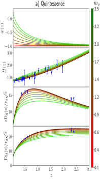
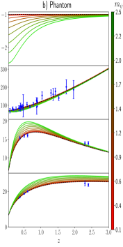
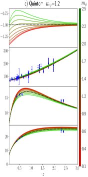
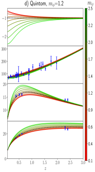
Figure 1: From left to right: quintessence, phantom and quintom cosmologies with potentials $V(\phi)=\frac{1}{2}m_{\phi}^{2}\phi^{2}$, $V(\psi)=\frac{1}{2}m_{\psi}^{2}\psi^{2}$ and $V(\phi,\psi)=\frac{1}{2}m_{\phi}^{2}\phi^{2}+\frac{1}{2}m_{\psi}^{2}\psi^{2}$, respectively. The first row displays the EoS $w(z)$, the second the Hubble function $H(z)$, the third the Hubble distance $D_{H}$ and the fourth the comoving angular distance $D_{M}$. The color bar represents different values for the masses of the fields. The data plotted for $H(z)$ correspond to the cosmic chronometers [47, 48, 49, 50, 51, 52, 53, 54]; for the $D_{H}$ and $D_{M}$ panels we use the BAO Galaxy consensus ($z\sim 0.5$) [55], Ly-$\alpha$ DR14 auto-correlation ($z=2.34$) [56] and cross-correlation ($z=2.35$) [57]. In all panles, the black dashed line describes the $\Lambda$CDM model.

Finally, in order to determine the dynamics of the system, it is necessary to solve the conservation equations for the matter components and scalar fields. Following [33], the Klein-Gordon equations can be rewritten as a dynamical system that can be solved straightforward, where the initial conditions for each field have been set up right into the matter domination epoch, and we have assumed a thawing behavior for the multi fields. This implies that at early times, the kinetic terms of the quintom model vanish, and its equation of state, $w_{Q}$, begins at $-1$. Also, the initial scalar field density parameter $\Omega_{Q,{\rm ini}}$ is selected, through a shooting mechanism, such that its present value satisfies the Friedmann constraint, $\Omega_{Q,0}+\Omega_{M,0}=1$. To illustrate the general behavior of the quintessence, phantom and quintom models, in Figure 1 we plot the following cosmological quantities: (from top to bottom) EoS $w(z)$, the Hubble function $H(z)$, the Hubble distance $D_{H}$ and the comoving angular distance $D_{M}$ along with several measurements (see the caption’s figure). In all the panels, the $\Lambda$CDM model is represented by a black dashed line. As a proof of the concept, the potentials used in our analysis are as followed: for quintessence and phantom the quadratic potential, and for quintom the sum of the two aforementioned potentials

$$\text{quintessence:}\quad V_{\phi} = \frac{1}{2}m_{\phi}^{2}\phi^{2},$$ (11)

$$\text{phantom:}\quad V_{\psi} = \frac{1}{2}m_{\psi}^{2}\psi^{2},$$ (12)

$$\text{quintom:}\quad V_{Q} = \frac{1}{2}m_{\phi}^{2}\phi^{2}+\frac{1}{2}m_{\psi}^{2}\psi^{2}.$$ (13)

Here $m_{\phi}$, $m_{\psi}$ are the masses of the fields; both of them plotted in units of [3$H_{0}$]. To show the main behavior of the inclusion of the fields, we varied only the masses and kept fix the rest of the cosmological parameters. Notice, that in general, for masses tending to null values we recover the $\Lambda$CDM pattern. In panels a) and b) of Figure 1, the quintessence model shows an EoS $w>-1$ meanwhile for phantom $w<-1$. Notice that, in both cases, as the masses of the fields increase, the EoS deviates farther from the cosmological constant line ($w=-1$) in the late–time regime, however in opposite directions. In general, all the quintessence $H(z)$ lines remain above the Hubble function of the $\Lambda$CDM model; this increment also yields to $D_{H}$ and $D_{M}$ to lay below the $\Lambda$CDM; for the phantom model occurs qualitatively the opposite. Both behaviors have been already studied in [33]. On the other hand, for the quintom model and without loosing generality, we considered two cases – panels c) and d) of Figure 1 –. In the first case we fix the phantom mass at $m_{\psi}=1.2$ and let the quintessence mass $m_{\phi}$ vary; while in the second case, we reversed the scenario. For a fixed $m_{\psi}$, panel c), the PDL crossing occurs when $m_{\phi}\gtrsim m_{\psi}$, and depending on the ratio $m_{\phi}/m_{\psi}$ the dark energy EoS presents a maximum which becomes more pronounced as $m_{\phi}/m_{\psi}$ increases; on the other hand, for a fixed $m_{\phi}$ the PDL crossing occurs less pronounced and the EoS may exhibit a minimum depending on the combination of $m_{\psi}/m_{\phi}$ . Finally, in these last two cases, there is a mixed behavior for $H(z)$, $D_{H}$ and $D_{M}$, to stay above or below to the $\Lambda$CDM observables, depending on the mass-parameter combination. In all cases the EoS converges to $w=-1$ at high redshift, by construction.

III Quintom model with interacting term

The previous section presented a quintom model with a non direct interacting term in the scalar field potential, i.e., it can be split up into two independent functions of the fields $V(\phi,\psi)=V(\phi)+V(\psi)$, therefore the Klein-Gordon eqs. (7) are coupled only through the Friedmann equation. Now, a step further is to consider a scalar potential with an interaction term. For a renormalizable model, a general form of the potential must include operators with dimension four or less, consisting of various powers of the scalar fields. A reasonable choice is to consider a potential which respects $Z_{2}$ symmetry, i.e., it is invariant under the following simultaneous transformations: $\phi\rightarrow-\phi$, $\psi\rightarrow-\psi$ [59]. A potential containing an interaction term between the fields $\phi$ and $\psi$ and with the above properties has the following form:

$$V(\phi,\psi)=\frac{1}{2}m_{\phi}^{2}\phi^{2}+\frac{1}{2}m_{\psi}^{2}\psi^{2}+\beta\phi^{2}\psi^{2}.$$ (14)

This is a particular case of the potential considered in Eq. (8) of Ref. [59] (see also Eq. (4) of Ref. [62]), when in the latter set the mass squared dimension’s constant $\Lambda_{0}=0$ and make the identification $\lambda^{2}=\beta$. Although phantom and, also, quintom models, as the one we are considering here (14), suffer from a severe problem of quantum instability [63, 64], it has been argued that, since we are considering a classical theory of gravity (GR), these fields should be considered as an appropriate effective description, no more.

Due to the interaction term, $\beta\phi^{2}\psi^{2}$, the equations of motion of the scalar fields are coupled, hence the term related to the potential in the Klein-Gordon equation of the field $\phi$ becomes $\frac{\partial V(\phi,\psi)}{\partial\phi}=m_{\phi}^{2}\phi+2\beta\phi\psi^{2}=f(\phi,\psi)$ which depends on both fields; the same happens for the $\psi$ field. We will refer to the quintom model with potential (14) as the interacting quintom, or just ‘quintom$+\beta$’. Although the above potential has been formerly considered to describe the qualitative behavior of a cyclic Universe [59, 62], as long as we know, its observational consequences have not been previously investigated in detail. This is one of the reasons why we chose this specific quintom model for our study. The other reason, which has been already commented in the text, is that quintom models provide a feasible crossing of the phantom divide, a feature that seems to be favored by the observations.

Figure 2 displays the quintom$+\beta$ potential for fixed values of the masses $m_{\phi}=1.5$ and $m_{\psi}=1.0$, and three values of the interaction constant $\beta=0.0,6.0,-2.0$. For the case $\beta=0$ we recover the results of the previous section. For positive $\beta$ there is a widen paraboloid with $V\geq 0$ whose minimum is at the region $\phi=\pm\frac{m_{\psi}}{m_{\phi}}\psi$, while in the negative $\beta$ case the potential may get to negative values (seen in the color bar of the figure), which can be problematic as they may produce a negative energy density. However, such behavior has been studied throughout negative dark energy models [65, 66, 67] and a sign switching cosmological constant $\Lambda$ [68, 69, 70, 71].

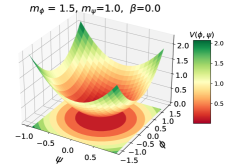
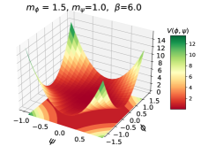
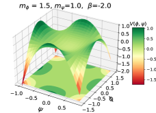
Figure 2: Quintom potential (expression (14)) for fixed values of the masses and positive, null and negative values of the coupling parameter $\beta$. The color bar indicates the values of the potential $V(\phi,\psi)$ ($z$-axis).

Let us explore some cosmological implications of the quintom$+\beta$ model by numerically solving the full dynamical system. Similarly to the previous cases, we compute the evolution of $w(z)$, $H(z)$, $D_{H}(z)$ and $D_{M}(z)$; their associated plots are shown in figure 3. In panel a) of this figure (fixed $m_{\psi}=1.2$, $\beta=4.0$ and varying $m_{\phi}$), the EoS at $w(z=0)$ is on the phantom region, grows up and reaches a local/global maximum value. If the mass ratio condition $m_{\phi}/m_{\psi}<1$ is satisfied (red lines), then the effective field evolves only in the phantom region, however for values $m_{\phi}\sim m_{\psi}$ it crosses to the quintessence regime, and in some combinations of the masses it is able to cross back into the phantom zone, therefore crossing twice the PDL. As the ratio $m_{\phi}/m_{\psi}$ increases (green lines), the maximum is shifted to larger redshifts and produces larger values of $w(z)$, to then remain in the quintessence region (the behavior of a Quintom-A field, as mentioned previously). An interesting point to note is that the quintom+$\beta$ model is able to traverse the Hubble $\Lambda$CDM line $H_{\Lambda{\rm CDM}}(z)$ (black dashed line). That is, if $H_{\Lambda{\rm CDM},0}$ is larger than the Hubble parameter given by the $H_{Q,0}$ of quintom+$\beta$ model, $H_{\Lambda{\rm CDM},0}>H_{Q,0}$, then at some redshift it will occur that $H_{\Lambda{\rm CDM}}(z)<H_{Q}(z)$. This type of behavior provides flexibility to transverse the $\Lambda$CDM observables $D_{H}(z)$ and $D_{M}(z)$, contrary to the decoupled quintom model (see panel c) and d) of figure 1).

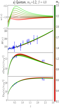
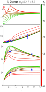
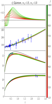
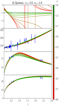
Figure 3: Quintom model. Two of the three parameters ($m_{\phi}$, $m_{\psi}$, and $\beta$) are fixed while the remaining varies in a range of values. From left to right, in the first panel vary $m_{\phi}$, in the second $m_{\psi}$, in the third $\beta\geq 0$ and in the fourth $\beta<0$. The first row is the EoS $w(z)$, the second the Hubble function $H(z)$, the third the Hubble distance $D_{H}$ and the fourth the angular distance $D_{M}$. The plotted data points are the same as in the Figure 1. The color bar represents different values for the masses of the fields or the $\beta$ parameter.

As the $\beta$ parameter increases (and depending on the combination of the masses) the oscillation is more pronounced and the crossing of the $\Lambda$CDM observables is more notorious, see for instance panel b) of figure 3 ($m_{\phi}=1.2$, $\beta=6.0$ and varying $m_{\psi}$). For $m_{\psi}/m_{\phi}<1$ (red lines), the EoS presents a wavering behavior and crosses the PDL multiple times. As the ratio $m_{\psi}/m_{\phi}$ increases, the number of oscillations are fewer with smaller amplitudes, until the evolution becomes a fully phantom behavior (green lines). A similar oscillatory function of $w(z)$ has been found by using non-parametric reconstructions directly from observables [4] and on phenomenological models that encompass these features [72]. Panel c) of figure 3 displays the outcomes for fixed mass values $m_{\phi}=1.5$, $m_{\psi}=1$ and taking only positive values of $\beta$. As the $\beta$ parameter increases the wavering behavior enhances, and both the crossing of the PDL and the maximum value of the EoS shift to higher redshifts.

Finally, in panel d) of figure 3 we show some peculiar behaviors when the negative case of $\beta$ is taken into account; here we use $m_{\phi}=2.0$ and $m_{\psi}=1$. At the present time, $w(z)$ resides in the quintessence region, opposite to the $\beta\geq 0$ case, but in the past, it crosses the PDL and for high negative values of $\beta$ the EoS diverges, to then come back to the region quintessence $w(z)>-1$ at early times. The presence of a pole in the EoS has been studied under several different physical circumstances in [73, 74, 75, 76, 77, 68, 65, 78, 79]. It is important to recall that $w(z)$ is not a physical observable, thus its divergence does not mean a physical pathology or an obvious constraint or failure of the model. The origin of the pole is clear from the definition of the barotropic EoS, $w=p/\rho$, which occurs when the energy density of the quintom dark energy density turns to be zero, i.e., when the negative terms of $\rho_{Q}=\frac{1}{2}(\dot{\phi}^{2}-\dot{\psi}^{2}+m_{\phi}^{2}\phi^{2}+m_{\psi}^{2}\psi^{2}-2|\beta|\psi^{2}\phi^{2})$ are relevant for certain values of $\beta$, such that $\rho_{Q}=0$, and hence $\rho_{Q}$ is able to change the sign to become negative. A negative energy density can be associated with the sign of the cosmological constant, the hypothesis of a negative mass, or just an effective energy density similar to the curvature case, see for instance [80, 81, 66, 69]. Regarding the Hubble function, it happens the opposite to the previous cases. If $H_{\Lambda{\rm CDM},0}$ is smaller than the Hubble parameter given by the quintom+$\beta$ model $H_{Q,0}$, that is $H_{\Lambda{\rm CDM},0}<H_{Q,0}$, then at some redshift it occurs that $H_{\Lambda{\rm CDM}}(z)>H_{Q}(z)$, and consequently the $D_{H}$ and $D_{M}$ traverse from bottom to top the $\Lambda$CDM line, as seen in the lower panels of the same figure.

IV Code and observations

We perform the parameter estimation and provide observational constraints from the latest data on the free parameters of the quintessence, phantom, quintom, and quintom+$\beta$ dark energy models considering the potentials (11), (12), (13) and (14), and discuss the model even further. In order to explore the parameter space, we use a modified version of dynesty, a library with several versions of the nested sampling algorithm. In conjunction, we utilize the SimpleMC cosmological parameter estimation code [82, 83], which computes expansion rates and distances using the Friedmann equation to calculate the posterior distributions. Equipped with these tools, we can easily calculate the Bayesian evidence $\ln\mathcal{Z}$, an informative measure of the compatibility of the statistical model with the observed data, thereby allowing direct comparison of two cosmological models, $a$ and $b$, using the Bayes factor $B_{ab}\equiv\mathcal{Z}_{a}/\mathcal{Z}_{b}$, or equivalently the relative log-Bayes evidence $\ln B_{ab}\equiv\Delta\ln\mathcal{Z}$. The model with smaller $|\ln\mathcal{Z}|$ is the preferred model, and to interpret the results, we refer to the Jeffreys’ scale: a weak evidence is indicated by $0\leq|\Delta\ln\mathcal{Z}|<1$, a moderate evidence $1\leq|\Delta\ln\mathcal{Z}|<3$, a strong evidence by $3\leq|\Delta\ln\mathcal{Z}|<5$, and a decisive evidence by $|\Delta\ln\mathcal{Z}|\geq 5$, in favor of the model. For an extended review of cosmological parameter inference see [84].

To perform the parameter estimation, we consider data from cosmic chronometers (HD), Type Ia supernovae (SN), and Baryon Acoustic Oscillation measurements (BAO), which are detailed in the following list:

• HD: Hubble distance measurements or cosmic chronometers are galaxies that evolve slowly and allow direct measurements of the Hubble parameter $H(z)$. We use the most recent compilation that contains a covariance matrix from Reference [85].

• SN: The SNeIa dataset used in this paper is the Pantheon+, a compilation of 1550 Type Ia supernovae within redshifts between $z=0.001$ and $z=2.26$ [86].

• BAO: High-precision Baryon Acoustic Oscillation measurements (BAO) at different redshifts up to $z<2.36$. We make use of the BAO data from SDSS DR12 Galaxy Consensus, BOSS DR14 quasars (eBOSS), Ly-$\alpha$ DR16 cross-correlation, Ly-$\alpha$ DR16 auto-correlation, Six-Degree Field Galaxy Survey (6dFGS) and SDSS Main Galaxy Sample (MGS) [87].

Throughout the analysis, we assume a flat FLRW universe, and flat priors over our sampling parameters: $\Omega_{{\rm m}0}=[0.05,1.0]$ for the pressureless matter density parameter today, $\Omega_{{\rm b}0}h^{2}=[0.02,0.025]$ for the physical baryon density parameter and $h=[0.4,1.0]$ for the reduced Hubble constant; additional to these parameters, for the quintom model we have $m_{\phi}=[0.0,4.0]$ the quintessence field mass, $m_{\psi}=[0.0,3.0]$ the phantom field mass and $\beta=[-10.0,10.0]$ for the coupling parameter, but when using the combination of all the datasets (BAO+HD+SN) we have used $\beta=[-2.0,4]$.

V Results

The main results of our analysis are shown in Table 1 where we report the constraints of the model parameters $\Omega_{m}$, $h$, $m_{\phi}$, $m_{\psi}$, $\beta$ along with 68% confidence level (CL), for all different combinations of the data sets: HD, SN, BAO, HD+SN, BAO+HD, BAO+SN, BAO+HD+SN. We also include the results of $\Lambda$CDM, as the reference model. Additionally, the same Table displays the best-fit, $-2\ln\mathcal{L}_{\rm max}$, along with the log-Bayesian evidence, $\ln\mathcal{Z}$, from the nested sampling algorithm, with the number of live-points selected using the general rule $50\times ndim$ [88], where $ndim$ is the number of parameters to be sampled from. Complementary to the table, in Figures 4 and 5, we display the two-dimensional marginalized distributions (the inner and external contours are for 68% and 95% CLs, respectively) and the constraints in the form of one-dimensional marginalized posterior distributions: figure 4 corresponds to quintessence and phantom dark energy, and figure 5 for quintom and quintom$+\beta$, in both cases we include the combination of datasets that provided the most constraining power.

In general, and among datasets, the Quintessence and Phantom models are statistically consistent with $\Lambda$CDM, however, there are some important points to mention. The quintessence model presents a nearly negligible improvement to describe datasets, that is, the comparison relative to the reference model is small $-2\ln\Delta\mathcal{L}_{\rm max}\lesssim 1$, except when both BAO and SN appear in the combined dataset, for these combinations, the improvement of the fit yield $-2\ln\Delta\mathcal{L}_{\rm max}\leq 2.85$. This can be understood by the lower $m_{\phi}$ values, which are accompanied by distinguishable values of $h$ compared to their counterpart in the $\Lambda$CDM model. Additionally from left panel of Figure 4 is evident that these datasets impose the tightest parameter constraints. Notice that the HD+SN combination gives the lowest $m_{\phi}$ value, nevertheless, for this reason, it is more capable of mimicking $\Lambda$CDM, carrying a barely different change in $h$ and a very similar fit. Consequently, the advantage of the additional parameter is lost. From the calculation of the Bayesian evidence, we can interpret that while $\Lambda$CDM is preferred over the quintessence model, this preference is generally weak for most of the data sets. However for SN and HD+SN, the evidence in favor of $\Lambda$CDM is definite but not strong.

In contrast to the quintessence model, the phantom model exhibits a positive correlation between $h$ and $m_{\psi}$ when considering the BAO and extra data, see left panel of Figure 4. However, in this model, the value of $-2\ln\Delta\mathcal{L}_{\rm max}$ does not show improvement compared to $\Lambda$CDM, even when for BAO+SN and BAO+HD+SN the constraints on the scalar field mass are more restrictive than the found for quintessence. Analyzing the Bayesian evidence, it suggests that while the phantom model, can be weakly or definitely less favored than $\Lambda$CDM, there is an exception for the HD sample, where it is indeed weakly favored. Notably, in this instance the parameter adjustment for $m_{\psi}$ exhibits the biggest value for this model.

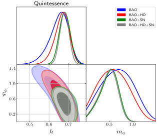
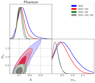
Figure 4: One- and two-dimensional (68% and 95% CLs) marginalized posterior distributions for the free parameters of quintessence (left) and phantom (right) dark energy models using BAO (blue), BAO+HD (red), BAO+SN (green) and BAO+HD+SN (gray).

On the other hand, when the two fields are incorporated into the quintom model, notice that with the inclusion of the BAO data, there is a positive correlation among the masses of the fields, but the correlation of the individual masses with the hubble parameter is essentially lost (see left panel of Figure 5). For all data combinations, the parameter adjustments favor $m_{\phi}>m_{\psi}$ indicating that the quintom model prefers to be dominated by the quintessence branch. Similar to the quintessence model, the fit is improved when the BAO and SN data appear in the dataset; in these cases $-2\ln\Delta\mathcal{L}_{\rm max}\leq 3.58$, and their corresponding $h$ value is lower than that obtained for $\Lambda$CDM. However, the penalization carried by the extra parameters is more evident when analyzing the Bayes factors. According to this criterion, it is notable that when only HD data is employed, both models have the same Bayes factor and then both are equally favored. For the BAO and BAO+HD combination, the quintom model is weakly disfavored compared to the standard model. Furthermore, for the remaining data combinations, the preference over $\Lambda$CDM is enhanced and now definitive. It is worth nothing that under the Bayesian evidence, even the BAO+SN and BAO+HD+SN combinations, which previously seemed to provide better fits, now are disfavored.

Now let us focus on the novel model, quintom$+\beta$. The first point to highlight is that the $\beta$ parameter is bounded by the different datasets, and even though the BAO and its combinations indeed provide tight constraints, with a slight preference for positive values of $\beta$, except for the SN data, all datasets and its combinations point out that $\beta=0$ is statistically admissible (the two-dimensional marginalized distributions of $\beta$ and $h$ are shown in the right panel of figure 6 for different combinations of datasets). Despite this fact, some important features come up with the introduction of this parameter. Some points to remark concerning the quintom+$\beta$ model are that, once again, the mass of the quintessence field is larger than the mass of the phantom field. This implies that, in this model as well, a preference exists for quintessence domination. It is also important to note that the masses of the fields are generally larger than those in the quintom model. In fact, for quintessence, all of them are greater than 1. In the right panel of Figure 5 we show the constraints of the quintom$+\beta$ model using BAO and additional datasets. A similar correlation occurs with the mass of the phantom and quintessence field (compared to the standard quintom model without coupling). This is an important point to stress out because now the datasets are in favor of $m_{\psi}$ different from zero with more than $2\sigma$ CL, in fact, the tightest constraint yields, $m_{\psi}=1.067\pm 0.214$ (BAO+HD+SN), which also yields to higher values of the quintessence mass $m_{\phi}=1.305\pm 0.533$ (BAO+HD+SN). To have a closer look of the correlations among the quintom$+\beta$ parameters, middle panel of figure 6 shows the 2D marginalized posterior distributions of $m_{\phi},m_{\psi}$ color coded with $\beta$ values. In this case, the most significant improvement to the fit occurs again when we consider the BAO+SN dataset (with $-2\ln\Delta\mathcal{L}_{\rm max}=3.56$ ). However, the results for the BAO+SN+HD combination are very close ($-2\ln\Delta\mathcal{L}_{\rm max}=3.28$ ). The inclusion of this coupling produces a difference in favor of the model that contributes to diminishing the BAO tension created between low redshift (galaxies) and high (Ly-$\alpha$) data, explored in [83, 68]. Even though this model contains three extra parameters, the Bayes factor, with respect to $\Lambda$CDM, highlights this aspect by imposing a more significant penalty compared to all the other models under consideration. However, this penalty is not high enough to discard the quintom+$\beta$ model, as $|\Delta\ln\mathcal{Z}|\leq 3.84$. Specifically the values of $|\Delta\ln\mathcal{Z}|$ indicate that when considering only HD data it is weakly disfavored; it is definitively disfavored for SN, BAO and BAO+SN combinations; and strongly disfavored by HD+SN, BAO+SN, and BAO+HD+SN dataset combinations. In a work in progress, for the quintom model with coupling, we are testing different potentials along with the Planck dataset (including linear perturbations), however for now, we are interested in the background cosmology.

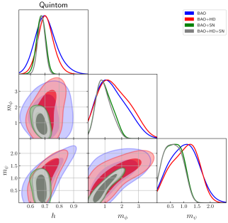
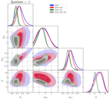
Figure 5: One- and two-dimensional (68% and 95% CLs) marginalized posterior distributions for the free parameters of quintom (left) and quintom$+\beta$ (right) dark energy models using BAO (blue), BAO+HD (red), BAO+SN (green) and BAO+HD+SN (gray).

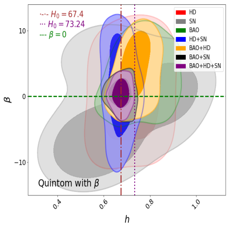
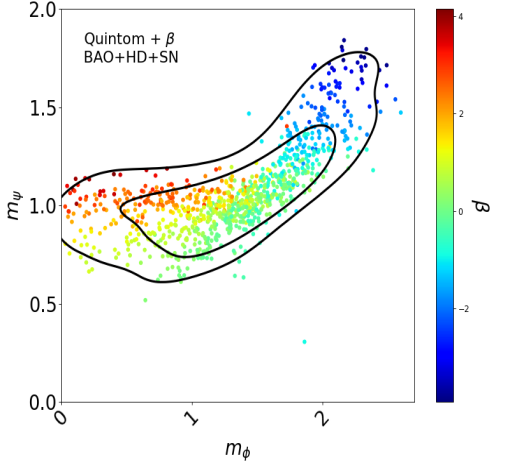
Figure 6: Quintom$+\beta$ model. Left panel: two-dimensional marginalized posterior distributions (68% and 95% CLs) $\beta-h$ plane for different combinations of datasets; the dashed lines correspond to the $\Lambda$CDM model: $H_{0}=73.24;$ km s^-1 Mpc^-1, coming from the Cepheid variables [89]; and $H_{0}=67.40;$ km s^-1 Mpc^-1, measured by the Planck mission [90]. Right panel: scatter plot in the $m_{\phi}-m_{\psi}$ plane for different values of $\beta$ (color bar), for BAO+HD+SN.

Once we have performed the parameter estimation, we are able to plot some derived probability distribution functions in order to look where are located the main deviations from the $\Lambda$CDM model. For instance, the left panel of figure 7 displays the Hubble function $H(z)/(1+z)$ and the right panel the dark energy equation of state (equation (6)). In this figure we present the results using BAO (top) and the combined BAO+HD+SN dataset (bottom), and also include the TRGB $H_{0}$ and BAO data points for comparison (red error bars). The solid lines represent 1$\sigma$ and 2$\sigma$ CLs and darker color means more likely as shown in the color bar; for comparison, the dashed blue line corresponds to the $\Lambda$CDM prediction. We observe there is a shift in the amplitude to lower values of $H(z)$, being clear for the case of BAO where almost the entire 1$\sigma$ region is lower than $\Lambda$CDM, and for the case of combined data this shift becomes small, as the constraints increased. Regarding the effective DE EoS, its best-fit value at $z=0$ is located below $w=-1$ (allowing small deviations incline to the phantom region), then it increases to cross the PDL and reaching a maximum value at about $z=0.5$, where the BAO-galaxy points are located, (also observed as an inverted bump in the $H(z)$ figure). Notice that at this redshift the quintom$+\beta$ model deviated by more than the $2\sigma$ region from the cosmological constant. After $w(z)$ has achieved the maximum value, it decreases to slightly cross back the PDL again; this may be an intent to fit the BAO-Ly$\alpha$ as well. For the case of joint data analysis we have a similar behavior but more constrained, with $w(z=0)\approx-1.1$ with a more restricted range but also favors the phantom region, the maximum is smaller too and throughout the redshift range $w=-1$ is acceptable. We must emphasize that the behavior presented by the EoS of the quintom$+\beta$ model with the values obtained from observational constraints (right panel of 7) is qualitatively similar to that obtained from model-independent reconstructions [17, 18, 4, 19], showing that the quintom with coupling is a plausible option to model the most recent observational results of dark energy.

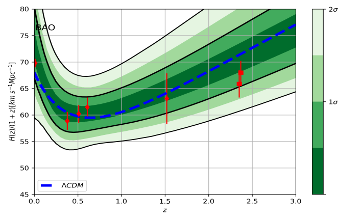
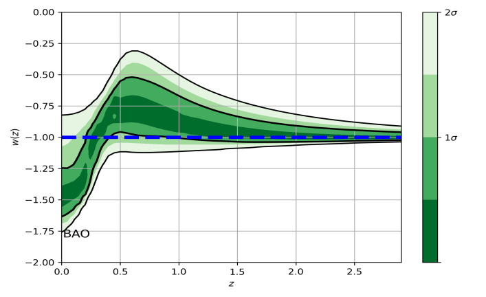
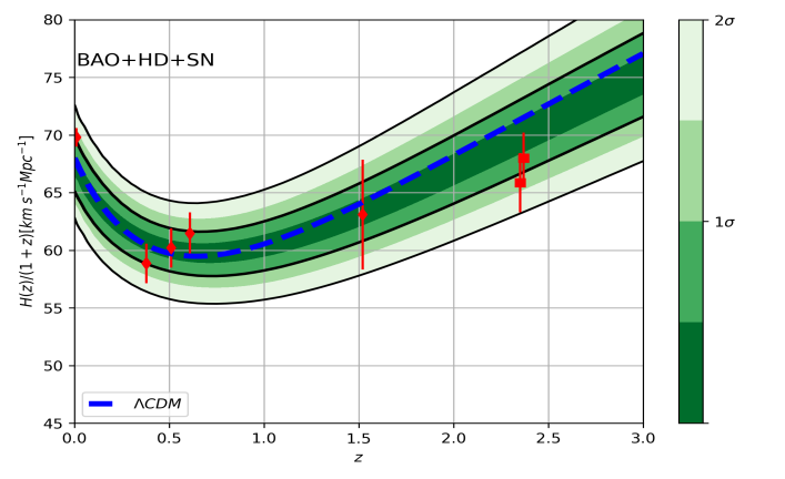
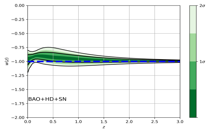
Figure 7: Cosmological functions derived from the posterior distributions using the quintom$+\beta$ model. Left: $H(z)/(1+z)$ and right the EoS parameter $w(z)$, using BAO (top) and BAO+HD+SN (bottom) datasets. The blue dashed lines represent the value of $\Lambda$CDM with the same parameter estimation as shown in the Table 1. The red error bars correspond to $H_{0}=69.8\pm 0.8$ km s^-1 Mpc^-1 from the TRGB [91], BAO Galaxy consensus ($z\sim 0.5$) [55], BOSS DR14 quasars (eBOSS, $z=1.52$) [92] and Ly-$\alpha$ DR16 and cross-correlation ($z=2.35$) and auto-correlation ($z=2.37$) [87].

VI Conclusions and Discussion

In this work, we have analyzed models of dark energy as minimally coupled scalar fields, specifically a quintessence and phantom models with quadratic potential eqs. (11) and (12), a quintom model as the sum of the quadratic potentials of the previous two fields Eq. (13); and a novel proposal, dubbed quintom$+\beta$ with sum of the quadratic potentials and an interaction term Eq. (14) inspired by [61]. Although quintessence and phantom with quadratic potential, as well as quintom as the sum of these, have been well-known models for some time, in order to make an update, in this work we constrained the parameters using late time data. Our main focus is to study the new proposal quintom$+\beta$, which enriches the quintom model in a simple way by adding only one extra degree of freedom to the usual non-minimal quintom model (the simplest coupling between the quintessence and phantom fields). We show that one of the main features of quintom$+\beta$ is that it produces a wavelike EoS (see figure 3) similar to the one reported in other works in other contexts [72]. When constraining the parameters, quintom$+\beta$ fits very well to the background cosmological data, specially for the SN, which exhibits a preferred negative $\beta$ value and results in an improvement of $-2\ln\Delta\mathcal{L}_{\rm max}=5.19$, compared to $\Lambda$CDM. This result leads to an EoS that starts, at early times, slightly below $-1$, then increases smoothly peaking at $z\approx 0.5$ and then decreases to end with a phantom value at present time $w(z=0)\approx-1.2$. Using the values of best fit, the CL for $H(z)$ and the EoS were calculated, the best fit of the parameters provides an EoS qualitatively similar to that reported by non-parametric reconstructions of dark energy [4] (see figure top right 7). As has already been said, this is precisely the behavior obtained from reconstructions, which allows us to say that quintom$+\beta$ with only one additional parameter to the two necessarily associated with the quintessence field and phantom, may reproduce the possible nature of the EoS obtained from observations. This makes the proposal of this work interesting, which motivates a more careful exploration of quintom models with potentials that couple the quintessence and phantom fields. It seems that interactions between fields through the product of powers of the fields, $V_{\rm int}\propto\phi^{n}\psi^{m}$, may play an important role in describing the dynamics of dark energy and may be a more economical way to add dynamics (several crosses to the PDL) instead of potentials with elaborated functions with a vaguely clear justification.

For four scalar field dark energy models (quintessence, phantom, quintom, quintom$+\beta$) and for $\Lambda$CDM (for comparison), the cosmological and model parameters were constrained using HD, SN and BAO data, and its combinations; in addition to calculating the Bayesian evidence. The observational constraints of the quintessence and phantom potential parameters associated to the mass of the fields, $m_{\phi}$ and $m_{\psi}$, give values for both around $m_{\phi,\psi}\approx 0.2-1.5$ and with a slight correlation with $h$ ($m_{\phi}$ directly proportional and $m_{\psi}$ inversely proportional). For the quintom model also the parameters are of the same order and slightly bigger than quintessence and phantom, $m_{\phi,\psi}\approx 0.6-1.8$; but in this case without correlation with $h$. For the proposed model quintom$+\beta$, the mass parameters are both $m_{\phi,\psi}\approx 1.0-2.06$ and the coupling parameter $\beta\approx-3.1-3.6$; it is noteworthy that in all cases the error bars of the constraints are of the order of the size for the mass parameters and even larger for the $\beta$ parameter. A natural improvement is to consider the CMB data and for a more detailed study consider linear perturbations.

The proposal to model the dark energy with quintessence and phantom scalar fields (to allow PLD crossing) with a potential with interacting term (to allow several crossings) seems to be reasonable since it is a flexible model that allows a dynamical EoS requiring three parameters (one for each field and one for the interaction) and with a simple functional form for the potential (polynomials). The quintom models are still valid as a candidate for dark energy; a deeper and more careful study on the origin of scalar fields is needed as well as better observational constraints.

Parameter	Datasets	Quintessence	Phantom	Quintom	Quintom$+\beta$	$\Lambda$CDM
$\Omega_{m}$	HD	$0.362\pm 0.120$	$0.346\pm 0.100$	$0.332\pm 0.103$	$0.346\pm 0.117$	$0.368\pm 0.108$
	SN	$0.306\pm 0.032$	$0.347\pm 0.026$	$0.309\pm 0.044$	$0.354\pm 0.083$	$0.332\pm 0.018$
	BAO	$0.300\pm 0.021$	$0.285\pm 0.020$	$0.276\pm 0.030$	$0.256\pm 0.033$	$0.292\pm 0.019$
	HD+SN	$0.311\pm 0.029$	$0.346\pm 0.024$	$0.311\pm 0.045$	$0.314\pm 0.084$	$0.332\pm 0.018$
	BAO+HD	$0.300\pm 0.019$	$0.287\pm 0.018$	$0.276\pm 0.030$	$0.252\pm 0.029$	$0.292\pm 0.018$
	BAO+SN	$0.300\pm 0.016$	$0.315\pm 0.014$	$0.296\pm 0.018$	$0.295\pm 0.018$	$0.313\pm 0.014$
	BAO+HD+SN	$0.301\pm 0.015$	$0.314\pm 0.014$	$0.298\pm 0.016$	$0.297\pm 0.016$	$0.312\pm 0.013$
$h$	HD	$0.630\pm 0.062$	$0.723\pm 0.083$	$0.722\pm 0.089$	$0.723\pm 0.088$	$0.661\pm 0.057$
	SN	$0.755\pm 0.162$	$0.737\pm 0.166$	$0.800\pm 0.141$	$0.671\pm 0.173$	$0.699\pm 0.174$
	BAO	$0.652\pm 0.048$	$0.739\pm 0.050$	$0.707\pm 0.074$	$0.747\pm 0.073$	$0.699\pm 0.022$
	HD+SN	$0.677\pm 0.040$	$0.674\pm 0.038$	$0.677\pm 0.038$	$0.673\pm 0.038$	$0.674\pm 0.040$
	BAO+HD	$0.667\pm 0.036$	$0.721\pm 0.033$	$0.707\pm 0.055$	$0.736\pm 0.048$	$0.696\pm 0.019$
	BAO+SN	$0.681\pm 0.027$	$0.709\pm 0.024$	$0.674\pm 0.031$	$0.674\pm 0.031$	$0.703\pm 0.023$
	BAO+HD+SN	$0.680\pm 0.023$	$0.702\pm 0.020$	$0.676\pm 0.025$	$0.675\pm 0.023$	$0.697\pm 0.019$
$m_{\phi}$	HD	$0.841\pm 0.524$	$-$	$1.780\pm 1.152$	$2.063\pm 1.062$
	SN	$0.493\pm 0.311$	$-$	$1.000\pm 0.660$	$1.383\pm 0.675$
	BAO	$0.664\pm 0.346$	$-$	$1.386\pm 0.867$	$1.636\pm 0.880$
	HD+SN	$0.409\pm 0.241$	$-$	$0.852\pm 0.534$	$1.461\pm 0.814$
	BAO+HD	$0.573\pm 0.326$	$-$	$1.514\pm 0.926$	$1.579\pm 0.864$
	BAO+SN	$0.492\pm 0.195$	$-$	$0.971\pm 0.466$	$1.313\pm 0.553$
	BAO+HD+SN	$0.473\pm 0.194$	$-$	$0.933\pm 0.443$	$1.305\pm 0.533$
$m_{\psi}$	HD	$-$	$1.496\pm 0.846$	$1.662\pm 0.786$	$1.788\pm 0.751$
	SN	$-$	$0.407\pm 0.307$	$0.713\pm 0.448$	$1.004\pm 0.515$
	BAO	$-$	$0.635\pm 0.466$	$0.989\pm 0.534$	$1.354\pm 0.370$
	HD+SN	$-$	$0.360\pm 0.243$	$0.628\pm 0.355$	$0.971\pm 0.360$
	BAO+HD	$-$	$0.502\pm 0.364$	$1.014\pm 0.506$	$1.297\pm 0.260$
	BAO+SN	$-$	$0.189\pm 0.140$	$0.601\pm 0.354$	$1.068\pm 0.247$
	BAO+HD+SN	$-$	$0.191\pm 0.137$	$0.586\pm 0.350$	$1.067\pm 0.214$
$\beta$	HD	$-$	$-$	$-$	$1.244\pm 5.413$
	SN	$-$	$-$	$-$	$-3.120\pm 5.525$
	BAO	$-$	$-$	$-$	$3.590\pm 3.504$
	HD+SN	$-$	$-$	$-$	$1.041\pm 4.771$
	BAO+HD	$-$	$-$	$-$	$4.344\pm 3.395$
	BAO+SN	$-$	$-$	$-$	$0.382\pm 1.548$
	BAO+HD+SN	$-$	$-$	$-$	$0.375\pm 1.476$
$-2\ln\mathcal{L}_{\rm max}$	HD	$6.11$	$5.40$	$4.87$	$4.39$	$6.11$
	SN	$1402.88$	$1403.12$	$1402.57$	$1397.92$	$1403.11$
	BAO	$9.06$	$9.45$	$7.80$	$7.34$	$9.46$
	HD+SN	$1409.13$	$1409.25$	$1409.13$	$1407.95$	$1409.23$
	BAO+HD	$15.63$	$15.87$	$14.15$	$13.41$	$15.87$
	BAO+SN	$1412.14$	$1414.97$	$1411.41$	$1411.43$	$1414.99$
	BAO+HD+SN	$1418.59$	$1421.4$	$1418.09$	$1418.11$	$1421.39$
$\ln\mathcal{Z}$	HD	$-8.75\pm 0.18$	$-7.67\pm 0.16$	$-7.76\pm 0.16$	$-8.31\pm 0.18$	$-7.76\pm 0.16$
	SN	$-707.47\pm 0.20$	$-707.57\pm 0.19$	$-708.01\pm 0.21$	$-708.82\pm 0.23$	$-706.05\pm 0.17$
	BAO	$-12.61\pm 0.23$	$-12.57\pm 0.22$	$-12.62\pm 0.23$	$-13.40\pm 0.24$	$-11.69\pm 0.21$
	HD+SN	$-712.61\pm 0.23$	$-712.61\pm 0.22$	$-713.22\pm 0.23$	$-714.57\pm 0.25$	$-711.10\pm 0.20$
	BAO+HD	$-16.01\pm 0.23$	$-16.29\pm 0.23$	$-16.21\pm 0.23$	$-16.98\pm 0.25$	$-15.25\pm 0.22$
	BAO+SN	$-715.48\pm 0.25$	$-717.12\pm 0.25$	$-716.18\pm 0.26$	$-717.95\pm 0.28$	$-714.81\pm 0.22$
	BAO+HD+SN	$-718.81\pm 0.25$	$-720.40\pm 0.25$	$-719.77\pm 0.26$	$-721.90\pm 0.29$	$-718.06\pm 0.22$
$\ln B_{m,\Lambda}$	HD	$-0.99$	$0.09$	$0$	$-0.55$	$0$
	SN	$-1.42$	$-1.52$	$-1.96$	$-2.77$	$0$
	BAO	$-0.92$	$-0.88$	$-0.93$	$-1.71$	$0$
	HD+SN	$-1.51$	$-1.51$	$-2.12$	$-3.47$	$0$
	BAO+HD	$-0.76$	$-1.04$	$-0.96$	$-1.73$	$0$
	BAO+SN	$-0.67$	$-2.31$	$-1.37$	$-3.14$	$0$
	BAO+HD+SN	$-0.75$	$-2.34$	$-1.71$	$-3.84$	$0$

Table 1: Constraints at 68% CL on the parameters, $-2\ln\mathcal{L}_{\rm max}$ and log-Bayesian evidence $\ln\mathcal{Z}$ for quintessence, phantom, quintom and quintom$+\beta$, using different datasets.

VII Appendix

The dynamics of quintom models with various potentials have also been explored using dynamical system techniques. One of the studied potentials consists of a sum of individual exponentials, without a direct coupling [93], and with a particular interaction potential between the phantom and quintessence fields in [94]:

$$V = V_{\phi 0}\,e^{-\lambda_{\phi}\kappa\phi}+V_{\psi 0}\,e^{-\lambda_{\psi}\kappa\psi}+V_{\rm int}(\phi,\psi).$$ (15)

For this potential the authors found that there is a future attractor dominated by the phantom field, indicating an EoS below $-1$ at late times. Their analysis also show that, the universe went through distinct stages that allowed the quintessence field to dominate $(w>-1)$ in the past. This implies that the model enables a transition across the PDL irrespective of whether there is a direct coupling between the fields or not. In reference [93], it is shown that a similar EoS behavior to the one associated with Eq.(15) can be achieved by the Eq.(13. However they exhibit that the sum of potentials with a quadratic scalar field in the exponents, given by

$$V = V_{\phi 0}\,e^{-\lambda_{\phi}\kappa^{2}\phi^{2}}+V_{\psi 0}\,e^{-\lambda_{\psi}\kappa^{2}\psi^{2}},$$ (16)

leads to an opposite behavior where the EoS transitions from being below $-1$ (at early times) to above $-1$ and tends to approach $-1$ at late times, this is similar to our findings for the quintom$+\beta$ with $\beta<0$ (see panel d) of figure 3). The EoS can also exhibit an oscillatory behavior. For instance, Figure 8 shows some cases when varying the mass of the field for the oscillatory potential

$$V=m_{\phi}^{2}(1-\cos(a\phi))+m_{\psi}^{2}(1-\cos(a\psi)).$$ (17)

Similar to the behavior of the Eq.(17), in reference [94], the authors argue that the following potentials can yield to an oscillatory EoS where the oscillations across $-1$ can occur in the recent past and have the potential to produce observable effects:

$$V = V_{1}\cos\left(\xi\frac{\phi}{M_{P}}\right)+V_{2}\cos\left(\beta\frac{\phi}{M_{P}}\right)+\beta\phi^{2}\psi^{2},$$ (18)

$$V = \frac{1}{2}m_{\phi}^{2}\phi^{2}+\frac{1}{2}m_{\psi}^{2}\psi^{2}+\beta\psi^{2}\phi^{2}.$$ (19)

Another combination of potentials that has been explored in the quintom scenario is the linear potential, [95, 96]:

$$V=a(\phi+\psi)+\beta\phi\psi\,.$$ (20)

By changing the sign of the coupling constant, $\beta$, the model is capable of emulating the distinct characteristics exhibited by both quintessence and phantom models, similar to our findings.

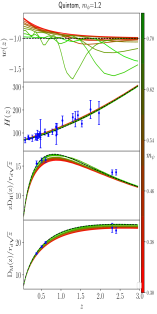
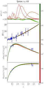
Figure 8: Quintom model with oscillatory potential. $w(z)$, $H(z)$, $D_{H}(z)$ and $D_{M}(z)$ for different values of the parameters $m_{\phi}$ for the oscillatory potential (17).

References

- Huterer and Shafer [2018] Dragan Huterer and Daniel L Shafer. Dark energy two decades after: Observables, probes, consistency tests. Rept. Prog. Phys., 81(1):016901, 2018. doi: 10.1088/1361-6633/aa997e.
- Abdalla et al. [2022] Elcio Abdalla et al. Cosmology intertwined: A review of the particle physics, astrophysics, and cosmology associated with the cosmological tensions and anomalies. JHEAp, 34:49–211, 2022. doi: 10.1016/j.jheap.2022.04.002.
- Copeland et al. [2006] Edmund J. Copeland, M. Sami, and Shinji Tsujikawa. Dynamics of dark energy. Int. J. Mod. Phys. D, 15:1753–1936, 2006. doi: 10.1142/S021827180600942X.
- Zhao et al. [2017] Gong-Bo Zhao et al. Dynamical dark energy in light of the latest observations. Nature Astron., 1(9):627–632, 2017. doi: 10.1038/s41550-017-0216-z.
- Sola Peracaula et al. [2019] Joan Sola Peracaula, Adria Gomez-Valent, and Javier de Cruz Pérez. Signs of Dynamical Dark Energy in Current Observations. Phys. Dark Univ., 25:100311, 2019. doi: 10.1016/j.dark.2019.100311.
- Wang et al. [2019] Deng Wang, Wei Zhang, and Xin-He Meng. Searching for the evidence of dynamical dark energy. The European Physical Journal C, 79(3):1–10, 2019.
- Chudaykin et al. [2021] Anton Chudaykin, Konstantin Dolgikh, and Mikhail M. Ivanov. Constraints on the curvature of the Universe and dynamical dark energy from the Full-shape and BAO data. Phys. Rev. D, 103(2):023507, 2021. doi: 10.1103/PhysRevD.103.023507.
- Yang et al. [2021] Weiqiang Yang, Eleonora Di Valentino, Supriya Pan, Yabo Wu, and Jianbo Lu. Dynamical dark energy after Planck CMB final release and tension. Mon. Not. Roy. Astron. Soc., 501(4):5845–5858, 2021. doi: 10.1093/mnras/staa3914.
- Di Valentino et al. [2021] Eleonora Di Valentino, Olga Mena, Supriya Pan, Luca Visinelli, Weiqiang Yang, Alessandro Melchiorri, David F. Mota, Adam G. Riess, and Joseph Silk. In the realm of the Hubble tension—a review of solutions. Class. Quant. Grav., 38(15):153001, 2021. doi: 10.1088/1361-6382/ac086d.
- Bahamonde et al. [2018] Sebastian Bahamonde, Christian G. Böhmer, Sante Carloni, Edmund J. Copeland, Wei Fang, and Nicola Tamanini. Dynamical systems applied to cosmology: dark energy and modified gravity. Phys. Rept., 775-777:1–122, 2018. doi: 10.1016/j.physrep.2018.09.001.
- Quiros [2019] Israel Quiros. Selected topics in scalar–tensor theories and beyond. Int. J. Mod. Phys. D, 28(07):1930012, 2019. doi: 10.1142/S021827181930012X.
- Tsujikawa [2013] Shinji Tsujikawa. Quintessence: A Review. Class. Quant. Grav., 30:214003, 2013. doi: 10.1088/0264-9381/30/21/214003.
- Ludwick [2017] Kevin J. Ludwick. The viability of phantom dark energy: A review. Mod. Phys. Lett. A, 32(28):1730025, 2017. doi: 10.1142/S0217732317300257.
- Chimento et al. [2006] Luis P. Chimento, Ruth Lazkoz, Roy Maartens, and Israel Quiros. Crossing the phantom divide without phantom matter. JCAP, 09:004, 2006. doi: 10.1088/1475-7516/2006/09/004.
- Cai et al. [2010a] Yi-Fu Cai, Emmanuel N Saridakis, Mohammad R Setare, and Jun-Qing Xia. Quintom cosmology: theoretical implications and observations. Physics Reports, 493(1):1–60, 2010a.
- Escamilla and Vazquez [2023] Luis A. Escamilla and J. Alberto Vazquez. Model selection applied to reconstructions of the Dark Energy. Eur. Phys. J. C, 83(3):251, 2023. doi: 10.1140/epjc/s10052-023-11404-2.
- Alberto Vazquez et al. [2012] J. Alberto Vazquez, M. Bridges, M. P. Hobson, and A. N. Lasenby. Reconstruction of the Dark Energy equation of state. JCAP, 09:020, 2012. doi: 10.1088/1475-7516/2012/09/020.
- Hee et al. [2017] S. Hee, J. A. Vázquez, W. J. Handley, M. P. Hobson, and A. N. Lasenby. Constraining the dark energy equation of state using Bayes theorem and the Kullback–Leibler divergence. Mon. Not. Roy. Astron. Soc., 466(1):369–377, 2017. doi: 10.1093/mnras/stw3102.
- Wang et al. [2018] Yuting Wang, Levon Pogosian, Gong-Bo Zhao, and Alex Zucca. Evolution of dark energy reconstructed from the latest observations. The Astrophysical Journal Letters, 869(1):L8, 2018.
- Panpanich et al. [2021] Sirachak Panpanich, Piyabut Burikham, Supakchai Ponglertsakul, and Lunchakorn Tannukij. Resolving hubble tension with quintom dark energy model. Chinese Physics C, 45(1):015108, 2021.
- Dai et al. [2018] Ji-Ping Dai, Yang Yang, and Jun-Qing Xia. Reconstruction of the Dark Energy Equation of State from the Latest Observations. Astrophys. J., 857(1):9, 2018. doi: 10.3847/1538-4357/aab49a.
- Hu [2005] Wayne Hu. Crossing the phantom divide: Dark energy internal degrees of freedom. Phys. Rev. D, 71:047301, 2005. doi: 10.1103/PhysRevD.71.047301.
- Feng et al. [2005] Bo Feng, Xiulian Wang, and Xinmin Zhang. Dark energy constraints from the cosmic age and supernova. Physics Letters B, 607(1-2):35–41, 2005.
- Cai et al. [2010b] Y.F. Cai, E.N. Saridakis, M.R. Setare, and J.Q. Xia. Quintom cosmology: Theoretical implications and observations. Physics Reports, 493:1–60, 2010b. doi: https://doi.org/10.1016/j.physrep.2010.04.001.
- Qiu [2010] Taotao Qiu. Theoretical aspects of quintom models. Modern Physics Letters A, 25(11n12):909–921, 2010.
- Zhang and Li [2021] Ming-Jian Zhang and Hong Li. Observational constraint on the dark energy scalar field. Chin. Phys. C, 45(4):045103, 2021. doi: 10.1088/1674-1137/abe0bf.
- Lazkoz et al. [2007] Ruth Lazkoz, Genly Leon, and Israel Quiros. Quintom cosmologies with arbitrary potentials. Phys. Lett. B, 649:103–110, 2007. doi: 10.1016/j.physletb.2007.03.060.
- Leon et al. [2018] Genly Leon, Andronikos Paliathanasis, and Jorge Luis Morales-Martínez. The past and future dynamics of quintom dark energy models. The European Physical Journal C, 78(9):1–22, 2018.
- Mishra and Chakraborty [2018] Sudip Mishra and Subenoy Chakraborty. Dynamical system analysis of quintom dark energy model. Eur. Phys. J. C, 78(11):917, 2018. doi: 10.1140/epjc/s10052-018-6405-9.
- Marciu [2016] Mihai Marciu. Quintom dark energy with nonminimal coupling. Phys. Rev. D, 93(12):123006, 2016. doi: 10.1103/PhysRevD.93.123006.
- Socorro et al. [2013] J Socorro, Priscila Romero, Luis O Pimentel, and M Aguero. Quintom potentials from quantum cosmology using the frw cosmological model. International Journal of Theoretical Physics, 52(8):2722–2734, 2013.
- Dutta et al. [2021] Sourav Dutta, Muthusamy Lakshmanan, and Subenoy Chakraborty. Quantum cosmology with symmetry analysis for quintom dark energy model. Phys. Dark Univ., 32:100795, 2021. doi: 10.1016/j.dark.2021.100795.
- Vázquez et al. [2021] J. Alberto Vázquez, David Tamayo, Anjan A. Sen, and Israel Quiros. Bayesian model selection on scalar -field dark energy. Phys. Rev. D, 103(4):043506, 2021. doi: 10.1103/PhysRevD.103.043506.
- Benisty and Guendelman [2019a] David Benisty and Eduardo I Guendelman. Two scalar fields inflation from scale-invariant gravity with modified measure. Classical and Quantum Gravity, 36(9):095001, 2019a.
- Navarro-Boullosa et al. [2023] Atalia Navarro-Boullosa, Argelia Bernal, and J. Alberto Vazquez. Bayesian analysis for rotational curves with -boson stars as a dark matter component. preprint arXiv:2305.01127, 5 2023.
- Téllez-Tovar et al. [2022] L. O. Téllez-Tovar, Tonatiuh Matos, and J. Alberto Vázquez. Cosmological constraints on the multiscalar field dark matter model. Phys. Rev. D, 106(12):123501, 2022. doi: 10.1103/PhysRevD.106.123501.
- Padilla et al. [2019] Luis E. Padilla, J. Alberto Vázquez, Tonatiuh Matos, and Gabriel Germán. Scalar Field Dark Matter Spectator During Inflation: The Effect of Self-interaction. JCAP, 05:056, 2019. doi: 10.1088/1475-7516/2019/05/056.
- Benisty and Guendelman [2019b] David Benisty and Eduardo I. Guendelman. Two scalar fields inflation from scale-invariant gravity with modified measure. Class. Quant. Grav., 36(9):095001, 2019b. doi: 10.1088/1361-6382/ab14af.
- Bamba et al. [2015] Kazuharu Bamba, Sergei D. Odintsov, and Petr V. Tretyakov. Inflation in a conformally-invariant two-scalar-field theory with an extra term. Eur. Phys. J. C, 75(7):344, 2015. doi: 10.1140/epjc/s10052-015-3565-8.
- Vázquez et al. [2020] J. Alberto Vázquez, Luis E. Padilla, and Tonatiuh Matos. Inflationary cosmology: from theory to observations. Rev. Mex. Fis. E, 17(1):73–91, 2020. doi: 10.31349/RevMexFisE.17.73.
- Bertolami et al. [2012] Orfeu Bertolami, Pedro Carrilho, and Jorge Páramos. Two-scalar-field model for the interaction of dark energy and dark matter. Physical Review D, 86(10):103522, 2012.
- Arvanitaki et al. [2010] Asimina Arvanitaki, Savas Dimopoulos, Sergei Dubovsky, Nemanja Kaloper, and John March-Russell. String axiverse. Physical Review D, 81(12):123530, 2010.
- Mehta et al. [2021] Viraf M Mehta, Mehmet Demirtas, Cody Long, David JE Marsh, Liam McAllister, and Matthew J Stott. Superradiance in string theory. Journal of Cosmology and Astroparticle Physics, 2021(07):033, 2021.
- Cicoli et al. [2022] Michele Cicoli, Veronica Guidetti, Nicole Righi, and Alexander Westphal. Fuzzy dark matter candidates from string theory. Journal of High Energy Physics, 2022(5):1–52, 2022.
- Gutiérrez-Luna et al. [2022] Eréndira Gutiérrez-Luna, Belen Carvente, Víctor Jaramillo, Juan Barranco, Celia Escamilla-Rivera, Catalina Espinoza, Myriam Mondragón, and Darío Núñez. Scalar field dark matter with two components: Combined approach from particle physics and cosmology. Physical Review D, 105(8):083533, 2022.
- Feng et al. [2006] Bo Feng, Mingzhe Li, Yun-Song Piao, and Xinmin Zhang. Oscillating quintom and the recurrent universe. Physics Letters B, 634(2-3):101–105, 2006.
- Jimenez et al. [2003] Raul Jimenez, Licia Verde, Tommaso Treu, and Daniel Stern. Constraints on the equation of state of dark energy and the hubble constant from stellar ages and the cosmic microwave background. The Astrophysical Journal, 593(2):622, 2003. doi: https://doi.org/10.1086/376595.
- Simon et al. [2005] Joan Simon, Licia Verde, and Raul Jimenez. Constraints on the redshift dependence of the dark energy potential. Physical Review D, 71(12):123001, 2005. doi: https://doi.org/10.1103/PhysRevD.71.123001.
- Stern et al. [2010] Daniel Stern, Raul Jimenez, Licia Verde, Marc Kamionkowski, and S Adam Stanford. Cosmic chronometers: constraining the equation of state of dark energy. i: measurements. Journal of Cosmology and Astroparticle Physics, 2010(02):008, 2010. doi: https://doi.org/10.1088/1475-7516/2010/02/008.
- Moresco et al. [2012] Michele Moresco, Licia Verde, Lucia Pozzetti, Raul Jimenez, and Andrea Cimatti. New constraints on cosmological parameters and neutrino properties using the expansion rate of the universe to . Journal of Cosmology and Astroparticle Physics, 2012(07):053, 2012. doi: https://doi.org/10.1088/1475-7516/2012/07/053.
- Zhang et al. [2014] Cong Zhang, Han Zhang, Shuo Yuan, Siqi Liu, Tong-Jie Zhang, and Yan-Chun Sun. Four new observational data from luminous red galaxies in the sloan digital sky survey data release seven. Res. Astron. Astrophys., 14(10):1221, 2014. doi: https://doi.org/10.1088/1674-4527/14/10/002.
- Moresco [2015] Michele Moresco. Raising the bar: new constraints on the hubble parameter with cosmic chronometers at . Monthly Notices of the Royal Astronomical Society: Letters, 450(1):L16–L20, 2015. doi: https://doi.org/10.1093/mnrasl/slv037.
- Moresco et al. [2016] Michele Moresco, Lucia Pozzetti, Andrea Cimatti, Raul Jimenez, Claudia Maraston, Licia Verde, Daniel Thomas, Annalisa Citro, Rita Tojeiro, and David Wilkinson. A 6% measurement of the hubble parameter at : direct evidence of the epoch of cosmic re-acceleration. Journal of Cosmology and Astroparticle Physics, 2016(05):014, 2016. doi: https://doi.org/10.1088/1475-7516/2016/05/014.
- Ratsimbazafy et al. [2017] AL Ratsimbazafy, SI Loubser, SM Crawford, CM Cress, BA Bassett, RC Nichol, and P Väisänen. Age-dating luminous red galaxies observed with the southern african large telescope. Monthly Notices of the Royal Astronomical Society, 467(3):3239–3254, 2017. doi: https://doi.org/10.1093/mnras/stx301.
- Alam et al. [2017] Shadab Alam, Metin Ata, Stephen Bailey, Florian Beutler, Dmitry Bizyaev, Jonathan A Blazek, Adam S Bolton, Joel R Brownstein, Angela Burden, Chia-Hsun Chuang, et al. The clustering of galaxies in the completed sdss-iii baryon oscillation spectroscopic survey: cosmological analysis of the dr12 galaxy sample. Monthly Notices of the Royal Astronomical Society, 470(3):2617–2652, 2017.
- de Sainte Agathe et al. [2019] Victoria de Sainte Agathe, Christophe Balland, Hélion Du Mas Des Bourboux, Michael Blomqvist, Julien Guy, James Rich, Andreu Font-Ribera, Matthew M Pieri, Julian E Bautista, Kyle Dawson, et al. Baryon acoustic oscillations at z= 2.34 from the correlations of ly absorption in eboss dr14. Astronomy & Astrophysics, 629:A85, 2019.
- Blomqvist et al. [2019] Michael Blomqvist, Hélion Du Mas Des Bourboux, Victoria de Sainte Agathe, James Rich, Christophe Balland, Julian E Bautista, Kyle Dawson, Andreu Font-Ribera, Julien Guy, Jean-Marc Le Goff, et al. Baryon acoustic oscillations from the cross-correlation of ly absorption and quasars in eboss dr14. Astronomy & Astrophysics, 629:A86, 2019.
- Cai et al. [2007] Yi-fu Cai, Hong Li, Yun-Song Piao, and Xin-min Zhang. Cosmic Duality in Quintom Universe. Phys. Lett. B, 646:141–144, 2007. doi: 10.1016/j.physletb.2007.01.027.
- Xiong et al. [2008] H.H. Xiong Xiong, Y.F. Cai, T. Qiu, Y.S. Piao, and X. Zhang. Oscillating universe with quintom matter. Physics Letters B, 666:212–217, 2008. doi: https://doi.org/10.1016/j.physletb.2008.07.053.
- Arias [2020] José Germán Salazar Arias. Fenomenología del modelo cosmológico so(1,1), 2020. URL https://repositorio.cinvestav.mx/bitstream/handle/cinvestav/3598/SSIT0016691.pdf?sequence=1.
- Pérez-Lorenzana et al. [2008] Abdel Pérez-Lorenzana, Merced Montesinos, and Tonatiuh Matos. Unification of cosmological scalar fields. Physical Review D, 77(6):063507, 2008.
- Cai and Saridakis [2011] Yi-Fu Cai and Emmanuel N. Saridakis. Non-singular Cyclic Cosmology without Phantom Menace. J. Cosmol., 17:7238–7254, 2011.
- Carroll et al. [2003] Sean M. Carroll, Mark Hoffman, and Mark Trodden. Can the dark energy equation-of-state parameter w be less than ? Phys. Rev. D, 68:023509, 2003. doi: 10.1103/PhysRevD.68.023509.
- Cline et al. [2004] James M. Cline, Sangyong Jeon, and Guy D. Moore. The Phantom menaced: Constraints on low-energy effective ghosts. Phys. Rev. D, 70:043543, 2004. doi: 10.1103/PhysRevD.70.043543.
- Akarsu et al. [2019] Özgür Akarsu, John D. Barrow, Charles V. R. Board, N. Merve Uzun, and J. Alberto Vazquez. Screening in a new modified gravity model. Eur. Phys. J. C, 79(10):846, 2019. doi: 10.1140/epjc/s10052-019-7333-z.
- Calderón et al. [2021] Rodrigo Calderón, Radouane Gannouji, Benjamin L’Huillier, and David Polarski. Negative cosmological constant in the dark sector? Phys. Rev. D, 103(2):023526, 2021. doi: 10.1103/PhysRevD.103.023526.
- Acquaviva et al. [2021] Giovanni Acquaviva, Özgür Akarsu, Nihan Katirci, and J. Alberto Vazquez. Simple-graduated dark energy and spatial curvature. Phys. Rev. D, 104(2):023505, 2021. doi: 10.1103/PhysRevD.104.023505.
- Akarsu et al. [2020] Özgür Akarsu, John D. Barrow, Luis A. Escamilla, and J. Alberto Vazquez. Graduated dark energy: Observational hints of a spontaneous sign switch in the cosmological constant. Phys. Rev. D, 101(6):063528, 2020. doi: 10.1103/PhysRevD.101.063528.
- Akarsu et al. [2021] Özgür Akarsu, Suresh Kumar, Emre Özülker, and J. Alberto Vazquez. Relaxing cosmological tensions with a sign switching cosmological constant. Phys. Rev. D, 104(12):123512, 2021. doi: 10.1103/PhysRevD.104.123512.
- Sen et al. [2022] Anjan A. Sen, Shahnawaz A. Adil, and Somasri Sen. Do cosmological observations allow a negative ? Mon. Not. Roy. Astron. Soc., 518(1):1098–1105, 2022. doi: 10.1093/mnras/stac2796.
- Malekjani et al. [2023] Mohammad Malekjani, Ruairí Mc Conville, Eoin Ó. Colgáin, Saeed Pourojaghi, and M. M. Sheikh-Jabbari. Negative Dark Energy Density from High Redshift Pantheon+ Supernovae. 1 2023.
- Tamayo and Vazquez [2019] David Tamayo and J. Alberto Vazquez. Fourier-series expansion of the dark-energy equation of state. Mon. Not. Roy. Astron. Soc., 487(1):729–736, 2019. doi: 10.1093/mnras/stz1229.
- Sahni and Shtanov [2005] Varun Sahni and Yuri Shtanov. Did the Universe loiter at high redshifts? Phys. Rev. D, 71:084018, 2005. doi: 10.1103/PhysRevD.71.084018.
- Tsujikawa et al. [2008] Shinji Tsujikawa, Kotub Uddin, Shuntaro Mizuno, Reza Tavakol, and Jun’ichi Yokoyama. Constraints on scalar-tensor models of dark energy from observational and local gravity tests. Phys. Rev. D, 77:103009, 2008. doi: 10.1103/PhysRevD.77.103009.
- Bauer et al. [2010] Florian Bauer, Joan Sola, and Hrvoje Stefancic. Dynamically avoiding fine-tuning the cosmological constant: The ’Relaxed Universe’. JCAP, 12:029, 2010. doi: 10.1088/1475-7516/2010/12/029.
- Sahni et al. [2014] Varun Sahni, Arman Shafieloo, and Alexei A. Starobinsky. Model independent evidence for dark energy evolution from Baryon Acoustic Oscillations. Astrophys. J. Lett., 793(2):L40, 2014. doi: 10.1088/2041-8205/793/2/L40.
- Gomez-Valent et al. [2015] Adria Gomez-Valent, Elahe Karimkhani, and Joan Sola. Background history and cosmic perturbations for a general system of self-conserved dynamical dark energy and matter. JCAP, 12:048, 2015. doi: 10.1088/1475-7516/2015/12/048.
- Ozulker [2022] Emre Ozulker. Is the dark energy equation of state parameter singular? Phys. Rev. D, 106(6):063509, 2022. doi: 10.1103/PhysRevD.106.063509.
- Adil et al. [2023] Shahnawaz A. Adil, Özgür Akarsu, Eleonora Di Valentino, Rafael C. Nunes, Emre Özülker, Anjan A. Sen, and Enrico Specogna. Omnipotent dark energy: A phenomenological answer to the Hubble tension. 6 2023.
- Petit and d’Agostini [2014] J. P. Petit and G. d’Agostini. Negative mass hypothesis in cosmology and the nature of dark energy. Astrophys. Space Sci., 354(2):2106, 2014. doi: 10.1007/s10509-014-2106-5.
- Visinelli et al. [2019] Luca Visinelli, Sunny Vagnozzi, and Ulf Danielsson. Revisiting a negative cosmological constant from low-redshift data. Symmetry, 11(8):1035, 2019. doi: 10.3390/sym11081035.
- Vazquez et al. [2021] JA Vazquez, I Gomez-Vargas, and A Slosar. Updated version of a simple mcmc code for cosmological parameter estimation where only expansion history matters. https://github.com/ja-vazquez/SimpleMC, 2021.
- Aubourg et al. [2015] Éric Aubourg, Stephen Bailey, Julian E Bautista, Florian Beutler, Vaishali Bhardwaj, Dmitry Bizyaev, Michael Blanton, Michael Blomqvist, Adam S Bolton, Jo Bovy, et al. Cosmological implications of baryon acoustic oscillation measurements. Physical Review D, 92(12):123516, 2015. doi: https://doi.org/10.1103/PhysRevD.92.123516.
- Padilla et al. [2021] Luis E Padilla, Luis O Tellez, Luis A Escamilla, and Jose Alberto Vazquez. Cosmological parameter inference with bayesian statistics. Universe, 7(7):213, 2021. doi: https://doi.org/10.3390/universe7070213.
- Moresco et al. [2020] Michele Moresco, Raul Jimenez, Licia Verde, Andrea Cimatti, and Lucia Pozzetti. Setting the stage for cosmic chronometers. ii. impact of stellar population synthesis models systematics and full covariance matrix. The Astrophysical Journal, 898(1):82, 2020.
- Brout et al. [2022] Dillon Brout, Dan Scolnic, Brodie Popovic, Adam G Riess, Anthony Carr, Joe Zuntz, Rick Kessler, Tamara M Davis, Samuel Hinton, David Jones, et al. The pantheon+ analysis: cosmological constraints. The Astrophysical Journal, 938(2):110, 2022.
- Alam et al. [2021] Shadab Alam et al. Completed SDSS-IV extended Baryon Oscillation Spectroscopic Survey: Cosmological implications from two decades of spectroscopic surveys at the Apache Point Observatory. Phys. Rev. D, 103(8):083533, 2021. doi: 10.1103/PhysRevD.103.083533.
- Speagle [2020] Joshua S Speagle. dynesty: a dynamic nested sampling package for estimating bayesian posteriors and evidences. Monthly Notices of the Royal Astronomical Society, 493(3):3132–3158, 2020.
- Riess et al. [2016] Adam G Riess, Lucas M Macri, Samantha L Hoffmann, Dan Scolnic, Stefano Casertano, Alexei V Filippenko, Brad E Tucker, Mark J Reid, David O Jones, Jeffrey M Silverman, et al. A 2.4% determination of the local value of the hubble constant. The Astrophysical Journal, 826(1):56, 2016. doi: https://doi.org/10.3847/0004-637X/826/1/56.
- Aghanim et al. [2020] Nabila Aghanim, Yashar Akrami, M Ashdown, J Aumont, C Baccigalupi, M Ballardini, AJ Banday, RB Barreiro, N Bartolo, S Basak, et al. Planck 2018 results-vi. cosmological parameters. Astronomy & Astrophysics, 641:A6, 2020. doi: https://doi.org/10.1051/0004-6361/201833910.
- Freedman et al. [2019] Wendy L Freedman, Barry F Madore, Dylan Hatt, Taylor J Hoyt, In Sung Jang, Rachael L Beaton, Christopher R Burns, Myung Gyoon Lee, Andrew J Monson, Jillian R Neeley, et al. The carnegie-chicago hubble program. viii. an independent determination of the hubble constant based on the tip of the red giant branch. The Astrophysical Journal, 882(1):34, 2019.
- Ata et al. [2018] Metin Ata, Falk Baumgarten, Julian Bautista, Florian Beutler, Dmitry Bizyaev, Michael R Blanton, Jonathan A Blazek, Adam S Bolton, Jonathan Brinkmann, Joel R Brownstein, et al. The clustering of the sdss-iv extended baryon oscillation spectroscopic survey dr14 quasar sample: first measurement of baryon acoustic oscillations between redshift 0.8 and 2.2. Monthly Notices of the Royal Astronomical Society, 473(4):4773–4794, 2018.
- Guo et al. [2005] Zong-Kuan Guo, Yun-Song Piao, Xinmin Zhang, and Yuan-Zhong Zhang. Cosmological evolution of a quintom model of dark energy. Physics Letters B, 608(3-4):177–182, 2005.
- Zhang et al. [2006] Xiao-Fei Zhang, Hong Li, Yun-Song Piao, and Xinmin Zhang. Two-field models of dark energy with equation of state across-1. Modern Physics Letters A, 21(03):231–241, 2006.
- Perivolaropoulos [2005] Leandros Perivolaropoulos. Constraints on linear negative potentials in quintessence and phantom models from recent supernova data. Phys. Rev. D, 71:063503, 2005. doi: 10.1103/PhysRevD.71.063503.
- Wu and Yu [2005] Puxun Wu and Hongwei Yu. Statefinder parameters for quintom dark energy model. International Journal of Modern Physics D, 14(11):1873–1881, 2005.