GraphFC: Customs Fraud Detection with Label Scarcity

Abstract.

Custom officials across the world encounter huge volumes of transactions. With increased connectivity and globalization, the customs transactions continue to grow every year. Associated with customs transactions is the customs fraud - the intentional manipulation of goods declarations to avoid the taxes and duties. With limited manpower, the custom offices can only undertake manual inspection of a limited number of declarations. This necessitates the need for automating the customs fraud detection by machine learning (ML) techniques. Due the limited manual inspection for labeling the new-incoming declarations, the ML approach should have robust performance subject to the scarcity of labeled data. However, current approaches for customs fraud detection are not well suited and designed for this real-world setting. In this work, we propose GraphFC (Graph neural networks for Customs Fraud), a model-agnostic, domain-specific, semi-supervised graph neural network based customs fraud detection algorithm that has strong semi-supervised and inductive capabilities. With upto 252% relative increase in recall over the present state-of-the-art, extensive experimentation on real customs data from customs administrations of three different countries demonstrate that GraphFC consistently outperforms various baselines and the present state-of-art by a large margin.

1. Introduction

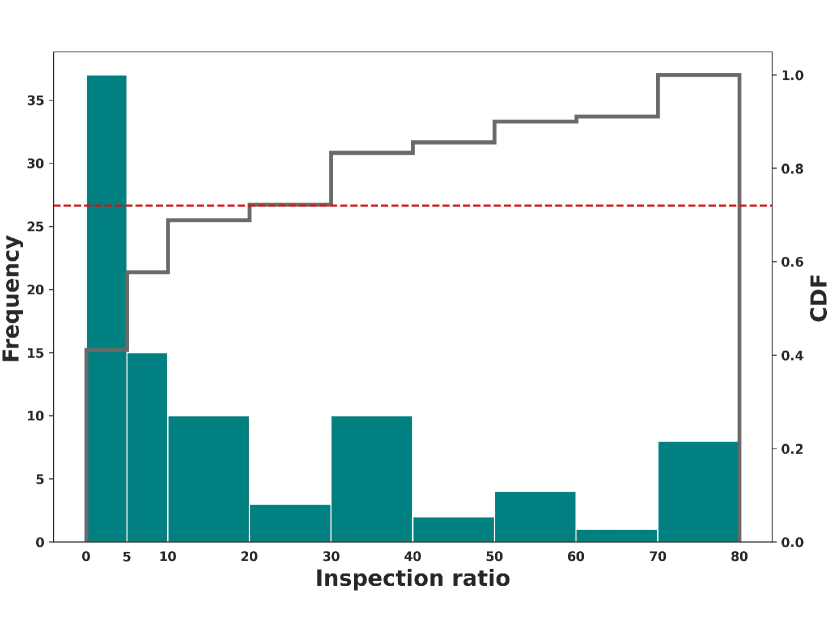
Figure 1. Distribution of physical inspection ratio among 90 countries across the world according to (Arvis et al., 2018). Around 72% countries have inspection rate less than 30%.

Customs is an authority in a country responsible for collecting tariffs and controlling the flow of goods into and out of country. According to the World Trade Organization, the world merchandise trade volume for exports and imports in 2019 alone was about 38 trillion dollars. With globalization and increased connectivity, the trade volumes continue to grow further.

Customs cover a wide range of trade facilitation issues aimed at greater transparency, effectiveness, and efficiency of government services and regulations with regard to the clearance of import, export and transit transactions across international borders. In addition to these aspects, customs also include facilitation measures relating to cross-border trade and supply-chain security. International trade and commerce via customs encounter malicious transaction declarations that involve intentional manipulation of trade invoices to avoid ad valorem taxes and duties (Mikuriya and Cantens, 2020; Keen, 2003; Cerioli et al., 2019). Administrators inspect trading goods and invoices to secure revenue generation from trades and develop automated systems to detect fraudulent transactions. This is an important undertaking as with customs transactions running into millions, even a slight increase in the detection accuracy will result in collection of hundreds of thousands of dollars of additional revenue. However, limited manpower and the colossal scale of trade volumes make the manual inspection of all transactions practically infeasible. In fact, as per the World Bank reports, administrations end up inspecting only a small portion, typically 5% or lower, of the total transactions (Geourjon et al., 2013; Arvis et al., 2018). To select the most suspicious transactions to be inspected, customs administrators often leverage rule-based algorithms or expert-systems with the domain know-how and empirical knowledge to determine the illicitness of transactions (Vanhoeyveld et al., 2020). Recently, the World Customs Organization (WCO) and its partner countries have made a great deal of progress in developing machine learning models, which can help officials identify and investigate any suspicious transactions that yield maximum revenue. For instance, India and China Customs Services applied decision tree and neural network based algorithms that outperform the traditional rule-based system (Shao et al., 2002; Kumar and Nagadevara, 2006). Moreover, the WCO had released DATE (Kim et al., 2020), a deep learning-based approach that jointly considers the information of importers and their trade goods and achieves state-of-the-art performance in detecting fraudulent transactions.

Although there are various approaches proposed for customs fraud detection, none of the existing work has addressed a critical issue: low inspection ratios and thereof lack of labeled ground-truth data for training the ML algorithms.

Figure 1 presents the distribution of physical inspection rate of 90 different countries across the world. Intuitively, we notice that around 40% of countries facilitate physical inspection less than 5% and up to 60% of countries has inspection rate less than 10%. Therefore, with low inspection ratio comes with the label scarcity. Scarcity of labeled data could severely hamper the performance of existing ML models for customs fraud detection models. We notice that most of the previous works and DATE (Kim et al., 2020; Shao et al., 2002; Kumar and Nagadevara, 2006), focus on a supervised learning paradigm that requires an adequately large amount of labeled data, which might become infeasible or less effective in fraud detection when dealing with limited labeled data.

To understand the impact of performance of existing approaches under different inspection ratios, we randomly sample n% of transactions from a fully labeled dataset ($\sim$2M labeled data) collected from a partner country of WCO (country B) and train supervised model learning models (e.g.,DATE and XGBoost). The results are presented in Figure LABEL:fig:performance_wrtInspection. We notice that supervised models achieve reasonably stable performance when the inspection rate is greater than 30%. However, in the case of inspection ratio lower than 30%, large number of data points become unlabeled and the performance drops significantly.

While the performance of a supervised ML model is limited by the scarcity of labeled data, the potential of utilizing heaps of unlabeled data in the customs domain has not been explored yet. Thus, in this work, we aim to mitigate the problem of label scarcity for ML driven customs fraud detection approaches by adopting a semi-supervised modeling approach.

To mitigate the difficulties arising from low inspection ratios, we propose a graph neural network (GNN) based customs fraud detection model and tackle this problem from the graph perspective. The setup can be viewed as a graph where the individual transactions act as nodes and form the network, and a pre-defined connectivity measure connects nodes, forming links in the network. For instance, if transaction $txn_{1}$ was made by importer $imp_{1}$ with the item coded $hs_{1}$, and importer id and item codes are defined to be the connectivity measures, links can be formed between transaction nodes as shown in Figure 3).

GNNs have been proven to have strong representational abilities in the semi-supervised setting (Kipf and Welling, 2017; Hamilton et al., 2017a; Ying et al., 2018; Velickovic et al., 2018). Moreover, self- and unsupervised pretraining approaches in GNNs enable learning of hidden relations and dynamics of interacting entities (Bojchevski and Günnemann, 2018; Veličković et al., 2018; Kipf and Welling, 2016). While learning the transactions representations, supervised approaches like XGBoost and DATE are not only incapable of such an unsupervised pretraining, but also of accommodating the information from neighboring transactions. In customs setting, the representations of transactions learnt by GNNs are enriched by amalgamating information from the linked transactions as well as the structure of the network.

Motivated by this, we propose Graph neural networks for Customs Fraud (GraphFC), a GNN-based customs fraud detection model operating on the structured customs data. The strength of GraphFC lies in its two-stage design. In the first stage, we employ self-supervised learning technique that jointly learns the representation among labeled and unlabeled data. The self-supervision process allows GraphFC understands the distribution of transactions and its related transactions throughout the message passing operation of GNN and the higher order connectivity in the transaction graph. Afterwards, in the second stage, we fine-tuned GraphFC with labeled data under a dual-task learning scheme which predicts the illicitness and the expected revenue simultaneously to make sure the most suspicious and valuable transaction could be detected and retrieved. The key finding of leveraging GNNs for fraud detection is it not only learns the knowledge from unlabeled data through self-supervised learning, but also capable of referring other associated transaction when making predictions. For instance, tradition models predict the illicitness of $txn_{1}$ solely based on the features derived from $txn_{1}$, while GraphFC takes the features of $txn_{1}$ and its relevant transaction $txn_{2},txn_{3}$ into account. We found that such design could substantially ease the performance drop with label scarcity and offer major improvements over strong baselines like XGBoost and the present state-of-the-art DATE model (Kim et al., 2020). The model code is made publicly available. We summarize our contributions as follows:

• We develop Graph neural networks for Customs Fraud (GraphFC) and showcase its strength in real-world customs fraud detection.

• GraphFC adopts self-supervised and semi-supervised learning techniques to extract rich information from unlabeled data, which substantially alleviate the performance degradation due to label scarcity.

• GraphFC optimizes on the dual of maximizing the detection of fraudulent transactions and maximizing the collection of associated revenue. Hence, it prioritizes fraudulent items that are likely to yield maximum penalty surcharge.

• Extensive experimentation on multi-year customs data from three countries shows that GraphFC outperforms the previous state-of-the-art and various other baselines.

2. Related Work

Most of the customs administrations are using legacy rule-based systems (Kültür and Çağlayan, 2017). Perhaps the biggest advantage of rule-based systems is their simplicity and interpretability. But rule systems are hard to maintain and are heavily dependent on expert knowledge (Pozzolo et al., 2018; Krivko, 2010). In general, advances in data science have led to the development of various fraud-detection models. A popular choice is tree-based models (Abdallah et al., 2016; West and Bhattacharya, 2016; Adewumi and Akinyelu, 2017; Ahmed et al., 2016).

Due to the non-availability of customs data in the public domain, the published literature on customs fraud is understandably scarce. However, there are some known efforts, like Belgium, where customs have tested an ensemble method of a support vector machine-based learner in a confidence-rated boosting algorithm (Vanhoeyveld et al., 2019); Columbia has demonstrated the use of unsupervised spectral clustering in detecting tax fraud with limited labels (de Roux et al., 2018); Indonesia customs have proposed an ensemble of tree-based approaches, support vector machine and neural network (Canrakerta et al., 2020). Similarly, Netherlands’ customs fraud detection model is built based on the Bayesian network and neural networks (Triepels et al., 2018). Another research employed a deep learning model to segregate high-risk and low-risk consignment on randomly selected 200,000 data from Nepal Customs of the year 2017 (Regmi and Timalsina, 2018). Other countries have developed their customs fraud detection systems such as Brazil (Filho and Wainer, 2008).

GNNs are being used in fraud detection. For instance (Zhu et al., 2020) addressed the homogeneity and heterogeneity of issue of networks for fraudulent invitation detection, anomaly detection on dynamic graphs with sudden bouts of increased and decreased activities is proposed in (Chen and Sun, 2020), (Wang et al., 2019a) proposed a semi-supervised approach and an attention-based approach for fraud detection in Alipay. In (Rao et al., 2020b), authors designed a dynamic heterogeneous graph from the users’ registrations to prevent the suspicious massive account registrations, (Dou et al., 2020) designs a GNN based fraud detection model to detect the camouflaged fraudsters, (Wang et al., 2019b) designs a graph convolutional network for fraudster detection in online app review system, (Rao et al., 2020a) undertakes the task of fraud detection in credit cards by learning temporal and location-based graph features.

Graph structure can also be defined as homogeneous, where nodes have the same set of features, such as the original GCN (Graph convolution network) (Kipf and Welling, 2017), where all the nodes (club members) have identical set features or are heterogeneous with nodes possessing a different set of features (Rao et al., 2020a; Schlichtkrull et al., 2018). While these approaches made advances in the GNN methodologies and applications, their application in customs domain is completely unexplored.

3. Problem Setting

3.1. Customs Selection

There are variety of customs fraud, but undervaluation is the most common type. Importers or exporters declare the value of their trade goods lower than the actual value, mainly to avoid ad valorem customs duties and taxes (Rodrigue et al., 2016). For this work, we limit the definition of an illicit customs transaction to that of undervaluation. Given the volume of transactions and limited resources to inspect them, the customs administration prioritizes items that entail a maximum penalty. In this light, we formulate the problem of customs selection as follows:

Problem: Given a transaction $o_{i}$ with its importer ID $imp_{i}$ and HS-code $c_{i}$ of the goods, the goal is to predict both the fraud score $\hat{y}_{i}^{cls}$ and the raised revenue $\hat{y}_{i}^{rev}$ obtainable by inspecting transaction $o_{i}$.

By selecting two predicted values, $\hat{y}_{i}^{cls}$ and $\hat{y}_{i}^{rev}$ in descending order from all transactions $O=\{o_{1},\ldots,o_{n}\}$ , customs administration could identify the most suspicious transactions $O_{F}\subset O$ to be inspected. Meanwhile, since we focus on mitigating the low inspection ratio problem in this work, we assume we have the labeled set $L=\{(x_{i},y_{i}^{cls},y_{i}^{rev}),\forall i=1,\ldots,n\}$ and unlabeled set $U=\{(x_{i}),\forall i=n+1,\ldots,m\}$, where $|L|\ll|U|$.

Note that we also exhibit the model performance in the supervised setting and leave the results in Appendix, although a very high inspection rate( $>$ 90%) is a rarity for customs administrations.

3.2. Transactions Graph from Tabular Data

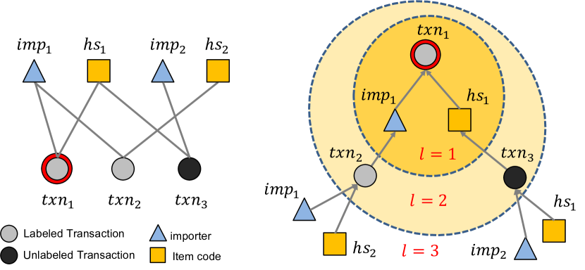
Figure 3. Transaction graph construction in GraphFC

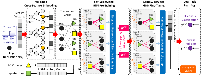
Figure 4. Model architecture of GraphFC. Cross features extracted from GBDT step act as node features in the transaction graph. In the pre-training stage, GraphFC learns the model weights and refine the transaction representations. Afterwards, the model is fine-tuned with labeled data with dual-task learning framework to predict the illicitness and the additional revenue.

One of the key insights of this work is to represent the customs transactions and their interactions as a graph and use GNNs to learn transaction-level embeddings by aggregating the neighborhood information. Traditional fraud detection methods (Kim et al., 2020; Vanhoeyveld et al., 2019; Filho and Wainer, 2008) judge the illicitness of a transaction solely depending on its features $x_{i}$ while the information of similar transactions is not considered.

We set up links (edges) between transactions (nodes) to capture any implicit patterns they might exhibit. These links could either be based on common categorical features, binned numerical features, or any other pre-defined rule. However, with even a relatively smaller customs office running into millions of transactions, we immediately run into a critical issue to exploding space complexity. A homogeneous graph formed by above rule suffers from a complexity of $O(n^{2})$ due to the pairwise relational nature, where $n$ denotes the number of transactions. To handle this issue, we introduce a set of virtual nodes $\mathcal{V_{C}}$ that are initially represented by the uniquely identifiable values/features (such as the importer id). Each node in $\mathcal{V_{C}}$ will only connect to transactions that share that feature value with it, and thus bringing down the space complexity from $O(n^{2})$ to $O(n)$.

Based on previous works like DATE (Kim et al., 2020), we choose importer ID and HS-code to be the categorical features defining the links between transactions. Thus, in this work, $\mathcal{V_{C}}$ is composed of the importer ID and HS-code with the uniquely identifiable values as their node IDs, as illustrated in the left half of Fig. 3. In line with this, when a prediction is made for a transaction $\bf{txn_{1}}$, the features of other transactions that share the same importer ID($\bf{txn_{2}}$) and HS-code($\bf{txn_{2}}$) would be propagated to $\bf{txn_{1}}$ to form a new representation, as demonstrated in the right side of Fig. 3. The detailed propagation rule will be described in Sec. 4. The transaction nodes $\mathcal{V_{T}}$ consist of both labeled and unlabeled transactions, which benefits the aggregation of additional information under a self- and semi-supervised setting.

The transaction graph could be represented as $\mathcal{G=(V,E)}$ where $\mathcal{V=V_{T}\cup V_{C}}$ is the node-set that denotes the combined individual transactions and the virtual nodes, and $\mathcal{E}$ denotes the connections between them based on the shared feature values. Let $\mathbf{D}\in\mathbb{R}^{h\times m}$ be the feature matrix that consists of $\mathbf{h=|\mathcal{V}|}$ nodes with their associated $\mathbf{m}$ features. It is worth noting that in the testing phase, only the historical transactions are considered for the inferring the transaction embedding. Also, the cross features from GBDT step become the features of nodes in $\mathcal{V_{T}}$, and the features of nodes in $\mathcal{V_{C}}$ are initialized with zero vectors $\vec{0}\in\mathbb{R}^{m}$.

4. Methodology

The proposed model GraphFC synergizes the strengths the GBDTs and GNNs. Model architecture for GraphFC is illustrated in Fig. 4, highlighting its multi-stage design.

4.1. Cross Features from GBDT

Tree-based methodologies are a popular choice for building machine learning models on tabular data. Tabular data is known to have hyperplane-like decision boundaries, and tree-based models allow for hyperplane-based recursive partitioning of data space, such that points in the partitioned space share the same class. In this work, we follow the feature extraction method using GBDTs as (Kim et al., 2020). Gradient Boosting Decision Trees (GBDTs) methodology can be understood as an ensemble technique where multiple weak learner models are combined to provide a powerful overall learner. The decision path in the fitted trees could be seen as a new set of features, with each path representing a new cross feature made from the original features. Assume $C$ and $E_{T}$ respectively represent internal nodes and their connecting paths in a decision tree $D_{T}$. $C$ further can be viewed as consisting of three sets of nodes, the root node $\{c_{R}\}$, internal nodes $C_{I}$, and the leaf nodes $C_{E}$, where $C=\{c_{R}\}\cup C_{I}\cup C_{E}$. Nodes in $c_{I}\in C_{I}$ splits features into some decision space. After passing through internal nodes, an input feature vector $\mathbf{x}\in\mathbf{X}$ gets assigned to a leaf node $l_{e}$. Then, a decision rule is the path connecting the root node to the leaf node. For instance, “gross.weight >100kg $\land$ quantity < 5” is a two-node decision path or a cross-feature comprising of features gross.weight and quantity.

Inspired by some recent studies such as (Wang et al., 2018; He et al., 2014), we utilize state-of-the-art XGBoost model (Chen and Guestrin, 2016) and extract cross features from the fitted model.

Let us assume $W$ represents the total number of leaves in the ensemble. An input vector $\mathbf{x}$ ends up in one of the leaf nodes according to the decision rules of each fitted decision tree. Each activated leaf node in the $t$-th decision tree can be represented as a one-hot encoding vector $\mathcal{F}_{t}$. We concatenate these together and produce a multi-hot vector $\mathbf{p}\in\mathbb{R}^{W}$, where $1$ indicates the activated leaves and $0$, the non-activated ones. After the extraction of cross features, we apply transformation for all data points to obtain a new feature matrix $\mathbf{M}\in\mathbb{R}^{n\times W}$.

4.2. Transaction Interaction Learning with Message Passing

The strengths of learning latent representations of transactions via graph neural networks are mainly threefold. First, given a transaction node $v_{t}\in\mathcal{V_{T}}$ and it’s representation vector $m^{k}_{t}$ at $k^{th}$ layer, graph neural network updates $m^{k}_{t}$ with the feature vector of adjacent nodes (i.e., $m_{j}^{k}~{}\forall j\in N(v_{t})$). Hence the nearby transactions in $\mathcal{G}$ could be included to form the representation for $v_{t}$. Second, the aggregation process takes the neighboring labeled and unlabeled transactions into account, a critical step in semi-supervised settings. Lastly, existing work (Kim et al., 2020) fails to extract informative patterns if either a new importer or an unseen item made the transaction. On the contrary, the inductive GNN generalizes to unseen nodes by exploring the node neighborhood. We elaborate the detailed framework in the following paragraphs.

In this work, GraphFC adopts GNN architecture inspired by GAT (Veličković et al., 2017), that has shown strong representation learning abilities among different graph learning tasks. Thanks to the flexible nature of our proposed approach, the backbone GNN architecture could be replaced with any GNN model. We demonstrate this by experimenting with GraphSAGE (Hamilton et al., 2017b) and RGCN (Schlichtkrull et al., 2018) (refer Table 2).

We initialize the node embedding for $\mathcal{V_{C}}$ with zero vectors then update it via the propagation from neighboring transaction features.

4.2.1. Local subgraph extraction via neighbor sampling

Training transductive GNNs such as GCN (Kipf and Welling, 2017) usually requires loading the entire graph data and the intermediate states of all nodes into memory. The full-batch training algorithm for GNNs suffers significantly from the memory overflow problem, especially when dealing with large scale graphs containing millions of nodes. Also, the addition of new nodes would require retraining of the entire model. To mitigate these issues, the neighborhood sampling technique (Hamilton et al., 2017b) is applied to extract a local subgraph from a target node for inductive mini-batch training. Specifically, it samples a tree rooted at each node by recursively expanding the root node’s neighborhood by $K$ steps with a fixed sample size of $\{T_{1},T_{2},...,T_{K}\}$, where $T_{i}$ is the number of nodes sampled in $i$-th step. Note that we alternately sample $T_{i}$ nodes from either $\mathcal{V_{C}}$ or $\mathcal{V_{T}}$ at each step to form the subgraph. Afterwards, the desired message passing operation could be applied to the subgraph.

4.2.2. Message passing with graph neural network

Intuitively, the interaction between nodes can be considered as an embedding propagation (i.e., message passing) from adjacent nodes to the source node. By stacking multiple message passing operations, the node representations collect information from a local subgraph, as illustrated in Fig. 3 and Sec. 3.2.

The process of message construction derives the joint representation of a node by passing its features through a neural network. The message aggregation process updates all of the neighboring messages obtainable from the previous message construction stage. It unifies them into a single representation as the final node embedding.

Message Construction. Given set of node pair $(m,j)$, where one of $\{m,n\}$ falls in $\mathcal{V_{T}}$ and the other belongs to $\mathcal{V_{C}}$. We first define the message from node $n$ to node $m$ as:

(1) $$g_{m\leftarrow j}=f(s_{m},s_{j}),$$

where $g_{m\leftarrow j}$ is the message embedding(i,e, information to be propagated) and $s_{k}$ denotes the $k^{th}$ row in $\mathbf{M}$. $f(\cdot)$ is the message encoding function which takes the node embeddings of $\{m,j\}$ and output their joint representation, $f(\cdot)$ is implemented as follows:

(2) $$f(s_{m},s_{j})=\alpha_{mj}s_{j},$$

where $\alpha_{mj}$ is the attention score that represents the similarity between nodes which is given as:

(3) $$\alpha_{mj}=\frac{\exp\left(\sigma\left(\mathbf{r}^{\top}[\mathbf{W}_{1}s_{j}\parallel\mathbf{W}_{1}s_{m}]\right)\right)}{\sum_{n\in N(m)}\exp\left(\sigma\left(\mathbf{r}^{\top}[\mathbf{W}_{1}s_{j}\parallel\mathbf{W}_{1}s_{j}]\right)\right)},$$

where $\mathbf{r}$ is the learnable vector that projects the embedding into a scalar, $\mathbf{\parallel}$ denotes the concatenation operation, $\sigma$ represents non-linear activation function(we use LeakyReLU (Maas et al., 2013) in this work), and $\mathbf{W}_{1}$ is a learnable weight matrix.

It is worth pointing out here that different GNN methods have various strategies to discriminate edges when generating node embeddings. In this work, we use attention-based aggregation to assign different importance weights to each edge so that the model can better distinguish transactions with different importers and with different HS-codes.

For example, RGCN (Schlichtkrull et al., 2018) exploits discriminate edges based on their relations, and SAGE (Hamilton et al., 2017b) does not discriminate edges but treat all links equal.

Thus, any newer aggregation methodologies can be employed in future for enhancing the performance even further.

Message Aggregation. In this stage, messages obtainable from node $m$ and all of it’s neighboring nodes $\{j\in N(m)\}$ are aggregated into an unified representation. Aggregation function is defined as:

(4) $$s_{m}^{(1)}=ReLU\left(g_{m\leftarrow m}+\sum_{j\in N(m)}\mathbf{W}_{2}~{}g_{m\leftarrow j}\right),$$

where $g_{m\leftarrow m}=W_{2}~{}s_{m}$ and $s_{m}^{(1)}$ denotes the new representation of node $m$ after the first propagation process and $W_{2}$ is a learnable weight matrix.

Given the first-order propagation rule (i.e., Eq. 4.2.2), we could further capture the higher-order transaction signals by stacking $k$ embedding propagation layer. Formally, the node representation at $k$-th layer could be derived as:

(5) $$\begin{split}s_{m}^{(k)}&=ReLU\left(g_{m\leftarrow m}^{(k)}+\sum_{j\in N(m)}\mathbf{W}_{2}^{(k)}~{}g_{m\leftarrow j}^{(k)}\right),\\ &=ReLU\left(\sum_{j\in N(m)\cup\{m\}}\mathbf{W}_{2}^{(k)}\alpha_{mj}^{(k)}s_{j}^{(k-1)}\right)\end{split}$$

where $W_{2}^{(k)}$ is a trainable matrix and $\alpha_{mj}^{(k)}$ is defined similar as Eq. 3 which $W_{1}$ is replaced by $W_{1}^{(k)}$ denotes the learnable weight matrix at the $k$-th layer. In this work, we use the embeddings at last layer (i.e., $s_{m}^{(k)}$) as the final representation for each transaction.

4.2.3. Order of Message Passing

In the message passing operation, one of the key components of GraphFC is to make use of the virtual node $\mathcal{V_{C}}$ to aggregate features from its neighboring transactions, with $\mathcal{V_{C}}$ being connected to both labeled and unlabeled transactions. As the node embeddings of virtual node $\mathcal{V_{C}}$ is initialized with zero vectors, it is critical to decide the order of message passing to avoid collecting information from an empty vector. We address this issue by updating embeddings of $\mathcal{V_{C}}$ and $\mathcal{V_{T}}$ in the following manner: In step 1, the embeddings for $\mathcal{V_{C}}$ are updated by collecting information from $\mathcal{V_{T}}$ via E.q 1. It is followed by step 2 that updates embeddings of $\mathcal{V_{T}}$ as per new representations of $V_{C}$. Step 1 and step 2 performed alternately to obtain the final embeddings.

4.3. Self-Supervised Pretraining

Unsupervised pretraining approaches in GNNs enable learning of hidden relational patterns and structural properties of the underlying network. The fact that such information can be learnt solely from observational data like node and edge features, without the need for ground-truth labels, lends an amazing flexibility to the representational learning of the GNNs (Bojchevski and Günnemann, 2018; Veličković et al., 2018; Kipf and Welling, 2016). Inspired by this, we adopt a self-supervised GNN pretraining scheme that learns transactions embeddings by using the given features of both the labeled and unlabeled transactions data.. Thereafter, we utilize these embeddings as a prior for the semi-supervised learning stage of GraphFC. The objective of the self-supervised step is to learn the embeddings of a node such that its representation in the latent space is closer to its neighboring nodes. By forcing the embedding of nearby nodes closer, GNN learns to preserve the graph structure level information as discussed in (Grover and Leskovec, 2016). Besides, it improves the generalization ability by aligning the distribution of unlabeled data closer to labeled data and thus reduce the extrapolation phenomenon.

We utilize the following self-supervised pretraining objective function (Hamilton et al., 2017b):

(6) $$\begin{split}\mathcal{L}_{pre}(s_{u}^{(k)})&=\frac{-1}{|N(u)|}\sum_{v\in N(u)}\log\left(\phi\left(s_{u}^{(k)\top}s_{v}^{(k)}\right)\right)\\ &+\frac{1}{R}\sum_{v_{n}\in P_{n}}\log\left(\phi\left(s_{u}^{(k)\top}s_{v_{n}}^{(k)}\right)\right)\end{split}$$

where $v$ is the immediate neighbor of node $u$, $P_{n}$ denotes the negative sampling distribution that gives a set of negative sampled nodes, and $R$ is the number of negative samples. By minimizing the objective function in Eq. 6, GraphFC is forced to lower the distance of representation of nearby nodes while pushing away the negative sampled nodes. Note that the pretraining operation is applied for all nodes in $\mathcal{V}$ which implies that both labeled and unlabeled information would be used to learn robust GNN parameters. Lastly, the trained parameters are saved and fine-tuned on the labeled dataset with Eq. 8.

4.4. Prediction and Optimization

To determine the illicitness of a given transaction, we propose to map the graph-based representation into scalars and train the neural network parameters via the following objective function. Inspired by (Kim et al., 2020), the dual-task learning framework is used to achieve two goals: 1. provide the probability of a transaction being illicit 2. predict the additional revenue (i.e., taxes) after inspecting suspicious transactions. Hence, we use the transaction representation (i.e., $s_{m}^{(k)}$) for both tasks of binary illicit classification and maximizing revenue prediction. Given the transaction feature $s_{m}^{(k)}$, we introduce the task-specific layer:

(7) $$\hat{y}^{cls}(s_{m}^{(k)}) =\phi\left(\mathbf{r}_{1}^{\top}s_{m}^{(k)}+\mathbf{b}_{1}\right),$$

$$\hat{y}^{rev}(s_{m}^{(k)}) =\mathbf{r}_{2}^{\top}s_{m}^{(k)}+\mathbf{b}_{2},$$

where $\textbf{r}_{1},\textbf{r}_{2}\in\mathbb{R}^{d}$ denotes the hidden vectors of task-specific layers that project $s_{m}^{(k)}$ into the prediction tasks of binary illicitness and raised revenue, respectively. $\phi$ is the sigmoid function. $\hat{y}^{cls}(s_{m}^{(k)})$ is the predicted probability of a transaction being illicit, and $\hat{y}^{rev}(s_{m}^{(k)})$ is the predicted raised revenue value of a transaction. The final objective function $\mathcal{L}_{\textsf{GraphFC}{}}$ is given by:

(8) $$\mathcal{L}_{\textsf{GraphFC}{}}=\mathcal{L}_{cls}+\alpha\mathcal{L}_{rev}+\lambda\|\Theta\|^{2},$$

where $\Theta$ denotes all learnable model parameters, $\mathcal{L}_{cls}$(refer Eq. 9) is the cross-entropy loss for binary illicitness classification, $\mathcal{L}_{rev}$ (refer Eq. 9) is the mean-square loss for raised revenue prediction. The hyperparameter $\alpha$ is used to balance the contributions.

Finally, we use mini-batch gradient descent to optimize the objective function $\mathcal{L}_{\textsf{GraphFC}{}}$, along with the Ranger (Wright, 2019) optimizer.

5. Evaluation

5.1. Experimental Setup

Table 1. Brief data description of the three datasets.

	A-Data	B-Data	C-Data
Starting Date	2016-01-01	2014-01-01	2017-01-01
Ending Date	2019-01-01	2017-01-01	2019-01-01
# Transactions	1895222	1428397	2385367
# importers	8699	165202	132893
# HS codes	5491	5953	13387
Overall Illicit rate	1.21%	4.12%	8.16%

We employed multi-year transaction-level import data from three partner countries, released by WCO for research usage. Because the data contains only the import transactions and those reported with undervaluation, we are only working with limited data from a larger dataset. Due to data confidentiality policies, we abbreviate these countries as A, B, and C. Subject to data availability, the three datasets have a different number of records, details of which are summarized in Table 1. Further, as data belongs to different customs administrations, it varies slightly in the features. Nonetheless, the most relevant features are the same across the datasets. Among others, these include the HS-code, importer ids, the notional value of the transaction, date, taxes paid, the quantity of the goods. We also include a binary feature representing historic fraudulent behavior or total taxes paid per unit value.

Data Split. To mimic the actual setting, we split the train, valid, and test data temporally. Since we have multi-year data, we treat the data from the most recent year as the test, and the older data is split as train and validation sets.

Because of our proposed design of introducing the virtual nodes for HS-codes and importer ids as presented in Sec 3.2, the number of edges in the resultant graph structures of each of the datasets would be twice the number of transactions in it.

Evaluation Criteria. The customs administrations can manually inspect only a limited number of transactions; we imitate this setting by evaluating the model performance on top-n% (we demonstrate results for 1%, and 5%) of the suspicious transactions suggested by the model. Thus, e.g., precision at 1% is equivalent to classification precision when top 1% of transactions suggested by GraphFC are manually inspected and the ground-truth for those transactions is obtained. Same as DATE (Kim et al., 2020), we use precision (Pre.), recall (Rec.) as evaluation metrics to inspect the model performance. As GraphFC supports the dual-task learning, we also report revenue (Rev.) collected by correct identification of the illicit transactions. This metric is reported as the ratio of the total revenue collected if all fraudulent transactions were identified. In a live setting, an inspection of top-n% items suggested by the model equates to customs officers examining the transactions that would yield the maximum revenue (refer Eq. 10).

We run an elaborate set of experiments that aim to answer the following: (a) Subject to the limited inspection rate by the customs officers, how well can GraphFC identify the fraudulent transactions? (b) Similarly, what additional revenue can GraphFC generate by inspection of items suggested by it? (c) How unlabeled data helps in semi-supervised learning? (d) Do different components in GraphFC contribute to making better predictions?, and finally, (e) Is the model robust to different backbone networks and inspection rates.

5.2. Performance Comparison

GraphFC performance is compared with 4 baseline methods:

• XGBoost (Chen and Guestrin, 2016): XGBoost is a tree-based model which is widely used for modeling tabular data.

• Tabnet (Arik and Pfister, 2019): Tabnet is a self-supervised learning-based framework especially designed for tabular data.

• VIME (Yoon et al., 2020): VIME adopts self-and semi-supervised learning techniques for tabular data modeling.

• DATE (Kim et al., 2020): This fraud detection method which utilizes tree-aware embeddings and attention network.

Table 2. Performance under 5% inspection rate. The 5% ground truth labels are used (95% of labels are masked). n denotes the top n% transaction suggested by the model.

A-Data
	n = 1%			n=5%
Model	Pre.	Rec.	Rev.	Pre.	Rec.	Rev.
XGB	0.026	0.021	0.040	0.017	0.070	0.096
Tabnet	0.031	0.024	0.031	0.016	0.061	0.049
VIME	0.021	0.018	0.030	0.007	0.030	0.038
DATE	0.045	0.037	0.056	0.033	0.129	0.187
$\textsf{GraphFC}{}_{\text{SAGE}}$	0.040	0.032	0.039	0.026	0.104	0.105
$\textsf{GraphFC}{}_{\text{RGCN}}$	0.050	0.040	0.064	0.039	0.152	0.189
GraphFC	0.045	0.035	0.057	0.030	0.118	0.170
B-Data
XGB	0.151	0.061	0.109	0.045	0.092	0.184
Tabnet	0.149	0.060	0.089	0.046	0.085	0.171
VIME	0.064	0.024	0.052	0.043	0.087	0.208
DATE	0.152	0.061	0.105	0.057	0.115	0.210
$\textsf{GraphFC}{}_{\text{SAGE}}$	0.327	0.132	0.143	0.201	0.405	0.305
$\textsf{GraphFC}{}_{\text{RGCN}}$	0.259	0.104	0.127	0.179	0.362	0.334
GraphFC	0.401	0.162	0.171	0.200	0.405	0.304
C-Data
XGB	0.671	0.070	0.120	0.445	0.234	0.359
Tabnet	0.715	0.050	0.081	0.452	0.231	0.334
VIME	0.725	0.076	0.116	0.471	0.249	0.362
DATE	0.803	0.085	0.158	0.472	0.249	0.380
$\textsf{GraphFC}{}_{\text{SAGE}}$	0.788	0.083	0.135	0.535	0.282	0.442
$\textsf{GraphFC}{}_{\text{RGCN}}$	0.819	0.086	0.146	0.525	0.277	0.424
GraphFC	0.869	0.092	0.170	0.535	0.282	0.445

Performance under Low Inspection Ratio. To verify the effectiveness of the proposed model subject to label scarcity, we assume a 5% inspection rate for each country and randomly sample 5% of the transactions from the train set as labeled and mask labels for the remaining 95% of the transactions. Results for this setting are presented in Table 2. Among the baseline methods, the current state-of-the-art customs fraud detection method, DATE, shows superiority due to its network design that considers the joint behavior between importer id and item codes. On the other hand, we notice that although VIME and Tabnet both utilize unlabeled data to perform self- and semi-supervised learning, the performance are still relatively lower than DATE and GraphFC. The reason being design of both DATE and GraphFC that explicitly consider the information of transactions made by different importers and trade goods. GraphFC shows a consistent and remarkable improvement over the baselines, which verifies the effectiveness of the proposed model. It is worth emphasizing that the significant improvement of GraphFC over VIME and Tabnet further validates the superiority of the proposed model.

Model Robustness. We demonstrate model robustness from two aspects: with different backbone GNNs, and by varying inspection rates. Specifically, we use the following backbone GNNs:

• $\textsf{GraphFC}{}_{\text{SAGE}}$: A GraphFC variant using GraphSAGE (Hamilton et al., 2017b) aggregator in message passing.

• $\textsf{GraphFC}{}_{\text{RGCN}}$: A GraphFC variant using RGCN (Schlichtkrull et al., 2018) aggregator designed for relational and heterogeneous graphs.

• GraphFC: Proposed model with GAT (Velickovic et al., 2018) based aggregator.

Inspection rates are varied in $\{1\%,2\%,5\%,10\%,20\%\}$, representing customs in different countries. Results with different backbone networks are presented in Table 2. Fig. LABEL:fig:varying_inspection shows the model performance under different inspection rates. It can be observed that though the detection performance drops as the inspection rate decreases, GraphFC and its variants still consistently outperform all the baselines. These results firmly establish that GraphFC is robust against different degrees of label scarcity, and generalize well in different countries. Additionally, model robustness with different backbone GNNs is a proof that any desired aggregation strategy can be used in GraphFC as per the features in the target data.

5.3. Effectiveness of Unlabeled Data

Table 3. Performance comparison on different training graphs under 5% inspection rate. n denotes the top n% transaction suggested by the model.

B-Data
	n = 1%			n=5%
Model	Pre.	Rec.	Rev.	Pre.	Rec.	Rev.
Q($\mathcal{G}_{L}$) + F($\mathcal{G}_{L}$)	0.245	0.099	0.134	0.147	0.298	0.259
Q($\mathcal{G}_{U}$) + F($\mathcal{G}_{L}$)	0.278	0.112	0.141	0.186	0.377	0.304
Q($\mathcal{G}$) + F($\mathcal{G}_{L}$)	0.286	0.115	0.141	0.180	0.363	0.285
Q($\mathcal{G}_{L}$) + F($\mathcal{G}$)	0.292	0.118	0.149	0.163	0.329	0.269
Q($\mathcal{G}_{U}$) + F($\mathcal{G}$)	0.402	0.162	0.155	0.173	0.349	0.286
Q($\mathcal{G}$) + F($\mathcal{G}$)	0.402	0.162	0.172	0.200	0.406	0.305

GraphFC improves its representation ability by utilizing the unlabeled data in the pretraining and fine-tuning stage. The key to making use of unlabeled data lies in the construction of transaction graph as presented in Fig. 3. The transaction graph comprises of $V_{T}$ and $V_{C}$, where $V_{T}$ includes both labeled and unlabeled transactions. To verify the effectiveness of unlabeled data in $V_{T}$, two variants of $\mathcal{G}$ are made with the following rule: (a) $\mathcal{G}_{L}$: keeps only the labeled transaction and its corresponding edges with $V_{C}$. (b) $\mathcal{G}_{U}$: keeps only the unlabeled transaction and its corresponding edges with $V_{C}$. We then compare the results using different graphs in the pretraining(Q) and fine-tuning (F) stage With 6 combinations and list the performance with a semi-supervised setting of B-Data in Table 3. Each row represents the graphs used in pretraining and fine-tuning, for example, $Q(\mathcal{G}_{L})+F(\mathcal{G}_{U})$ means pretraining with graph $\mathcal{G}_{L}$ and fine-tune on graph $\mathcal{G}_{U}$.

First, it is worth noticing that $Q(\mathcal{G}_{L})+F(\mathcal{G}_{L})$ is the only variant that solely uses labeled data without inclusion of any unlabeled data in the training process. The results show that it performs the worst among all test cases. The takeaway here is that the using unlabeled data in the pretraining or fine-tuning process leads to a significant improvement in the model performance. Second, we compare the result of fine-tuning on $\mathcal{G}_{L}$ and $\mathcal{G}$. The results show that fine-tuning with unlabeled data generally performs better, which again shows the advantage of jointly considering labeled and unlabeled information. Lastly, we observe the difference between $Q(\mathcal{G}_{L})$ , $Q(\mathcal{G}_{U})$ and $Q(\mathcal{G})$. $Q(\mathcal{G}_{L})$ is significantly worse than the others while $Q(\mathcal{G}_{U})$ and $Q(\mathcal{G})$ usually gives similar performance. This final result adds to the already evident effectiveness of adding unlabeled data in the pretraining stage. It not only provides more training instances for learning the weight matrices (i.e., $\mathbf{W}_{1}^{(k)},\mathbf{W}_{2}^{(k)}$) but makes the nearby transaction closer in embedding space, leading to better predictive capabilities.

To further explore the effect of including unlabeled data in GraphFC, we train two variants of GraphFC and mapped their transaction embedding obtainable before the output layer into 2-dimensional space using TSNE, and present the result in Figure LABEL:fig:tsne_plot. Figure LABEL:subfig:L_tsne presents the variant of GraphFC where we remove all of the unlabeled data in $\mathcal{G}$ (refer to the setting of $Q(\mathcal{G}_{L})+F(\mathcal{G}_{L})$), whereas for Figure LABEL:subfig:nopretrian_tsne, the pretraining step is ommited, and Figure LABEL:subfig:LU_tsne is the result of GraphFC. Figure LABEL:subfig:LU_tsne is the best performing case where legitimate and illicit transactions are separated well into two tightly clustered sets. In Figure LABEL:subfig:L_tsne, we can observe diverse patterns that are not clearly separable. Figure LABEL:subfig:nopretrian_tsne has better separation but data points are more dispersed than as compared to Figure LABEL:subfig:LU_tsne. To sum up, this analysis shows the importance of unlabeled data in learning high quality embedding vectors that played a key role for mitigating effects of label scarcity.

5.4. Prediction Performance for Unseen Importers

Inductive learning can be understood as the ability of the model to learn from the historic data and generalize it to new, unseen cases. Given the huge volume of transactions, the model will consistently come across input data that has unseen features, such as new items and importers. In the previous work DATE (Kim et al., 2020), the representations for every importer and HS-code were learnt, however, in a semi-supervised setting, such a learning becomes infeasible. GraphFC provides a novel solution for inductive learning by linking the newly observed importer and item to the target transaction and its representation could be updated via multiple messages passing operation. To measure the degree of the inductive phenomenon, we introduce Out-of-Sample-Ratio (OSR), which is defined as: $OSR=|P_{un}|/(|P_{s}|+|P_{un}|),$ where $|P_{s}|$ and $|P_{un}|$ denote the number of unique states (refer inductive setting in 3.1 for definition) observed and unobserved in the training data, respectively. The higher OSR is, the more unseen data states are present in the data. In this work, we focus on analyzing the behavior of importer and HS-code.

Table 4. Inductive setting - Importer

A-Data, OSR: 9.89%
	n = 1%			n=5%
Model	Pre.	Rec.	Rev.	Pre.	Rec.	Rev.
GraphFC	0.0486	0.0168	0.0161	0.0396	0.0686	0.0672
DATE	0.0660	0.0229	0.0271	0.0501	0.0866	0.0953
B-Data, OSR: 49.43%
GraphFC	0.5386	0.1963	0.2236	0.2055	0.3744	0.3846
DATE	0.0655	0.0239	0.0482	0.0549	0.1000	0.1580
C-Data, OSR: 5.09%
GraphFC	0.9052	0.0483	0.0847	0.7805	0.2081	0.3396
DATE	0.7730	0.0413	0.0616	0.6418	0.1711	0.2605

Table 5. Inductive setting - HSCode

A-Data, OSR: 2.75%
	n = 1%			n=5%
Model	Pre.	Rec.	Rev.	Pre.	Rec.	Rev.
GraphFC	0.0560	0.0329	0.0219	0.0471	0.1382	0.1213
DATE	0.0373	0.0219	0.0104	0.0396	0.1162	0.0964
B-Data, OSR: 3.64%
GraphFC	0.4554	0.1053	0.1256	0.1577	0.1808	0.1889
DATE	0.2772	0.0641	0.1002	0.0978	0.1121	0.1960
C-Data, OSR: 4.74%
GraphFC	0.7320	0.0574	0.1143	0.4277	0.1675	0.2620
DATE	0.5876	0.0461	0.0933	0.3946	0.1545	0.2142

Inductive analysis in semi-supervised learning We evaluate the performance of inductive learning by selecting a subset of transactions from testing data where the importer ID or HS-code were not observed in training data. The result is presented in and presents the result in Table 4 and 5. We compare GraphFC with DATE as DATE being the state-of-the-art method for transductive learning. In Table 4, it demonstrates the performance on predicting transactions made by unseen importers. GraphFC outperforms DATE with a significant improvement as OSR increases. Especially in B-data, the OSR is 49.43% and GraphFC gains 7x improvement in terms of Pre@1%. On the other hand, Table 5 also shows the superiority against DATE on unseen HS-code. Additionally, in Figure 7 we also show the effect of varying OSR rates by controlling HS codes and importer id. GraphFC outperforms the baselines in all cases.

Figure 7. Performance comparison by varying OSR (%). (a) & (b) & (c) (controls importer id), (d) & (e) & (f) (controls HS-code). In all cases, GraphFC outperforms the baselines.

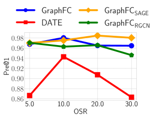
(a) N-data

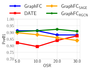
(b) T-data

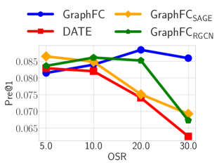
(c) C-data

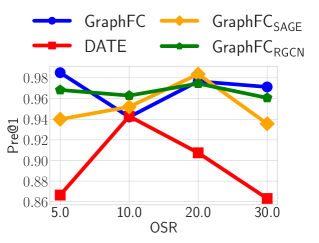
(d) N-data

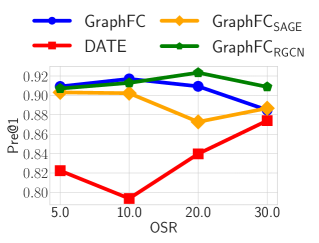
(e) T-data

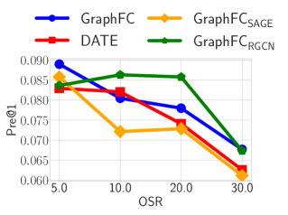
(f) C-data

5.5. Component Analysis

Table 6. Component Analysis.

A-Data
	n = 1%			n=5%
Model	Pre.	Rec.	Rev.	Pre.	Rec.	Rev.
GraphFCsemi	0.030	0.024	0.034	0.023	0.092	0.127
GraphFCjoint	0.025	0.019	0.037	0.023	0.090	0.117
GraphFConly	0.032	0.024	0.034	0.017	0.067	0.081
GraphFCsparse	0.030	0.024	0.037	0.018	0.070	0.096
GraphFC	0.045	0.035	0.057	0.030	0.118	0.170
B-Data
GraphFCsemi	0.281	0.113	0.162	0.197	0.398	0.367
GraphFCjoint	0.218	0.076	0.092	0.105	0.203	0.212
GraphFConly	0.068	0.027	0.069	0.034	0.069	0.157
GraphFCsparse	0.067	0.070	0.120	0.044	0.234	0.359
GraphFC	0.401	0.162	0.171	0.200	0.405	0.304
C-Data
GraphFCsemi	0.829	0.087	0.143	0.548	0.289	0.434
GraphFCjoint	0.807	0.061	0.135	0.491	0.249	0.401
GraphFConly	0.764	0.080	0.115	0.490	0.258	0.382
GraphFCsparse	0.712	0.075	0.123	0.473	0.250	0.376
GraphFC	0.869	0.092	0.170	0.535	0.282	0.445

To establish the contribution of different components in GraphFC, we ablate its core components and evaluate its performance. Specifically, we evaluate the following settings:

• GraphFC: Use full model.

• No unsupervised pretraining (GNN_semi): Skip the unsupervised pre-train step.

• Joint training (GNN_joint): Remove pretraining and jointly optimizing E.q 6 and Eq. 8.

• No GBDT (GNN_only): Remove the GBDT step of the model and utilize the data from transactions directly.

• No item/importer nodes (GNN_sparse): Remove one of the categorical nodes utilized for building the graph structure and build a sparser graph.

Results of different variants are demonstrate in Table 6. It can be noticed that removing any component in GraphFC leads to degradation of performance. The only exception is for GraphFC_semi that delivers similar performance in C-data. Among these variants, GraphFC_sparse and GraphFC_only perform poorly which indicates that both the GBDT step, and utilizing the importer and HS-code for constructing the transaction graph play an important role in GraphFC.

In general, neither GraphFC_semi nor GraphFC_joint improves GraphFC which verifies the necessity our pretraining step. Specifically, the difference between GraphFC and GraphFC_semi, GraphFC_joint are significant when $n$ is small (e.g. $n=1\%$) which is important since customs usually maintain a low inpsection rate lower than 5%.

6. Discussion and Conclusion

With increased connectivity, development, and globalization, customs administrations across the world have to process an increasingly large number of transactions. This calls for an automated system for detecting fraudulent transactions, as manual inspection of such an astronomical volume of transactions is infeasible. In this work, we develop GraphFC, a GNN based fraud detection model that transforms the customs tabular data into a graph and maximizes the identification of malicious customs transactions while also maximizing the additional revenue collected from these transactions. We propose the given approach and exhibit its effectiveness by developing a model and testing it on real data from multiple countries. In our experiments, we show that GraphFC is capable of making use of the precious unlabeled data and further substantially alleviate the performance drop under different levels of label scarcity. The proposed model provides a remedy to any country who is trying to facilitate automated customs fraud detection even if the administration did not collect huge labeled data.

Appendix A Appendix

A.1. Algorithm and Complexity Analysis

Input: Graph $\mathcal{G(V,E)}$; node feature matrix $\mathbf{D}$; depth $K$; learnable weight matrices $\Theta=\{\mathbf{W}_{1}^{(k)},\mathbf{W}_{2}^{(k)},\forall k\in\{1,...,K\}$

, $\mathbf{r}_{1},\mathbf{r}_{2}\}$; labeled data $L=(x_{i},y_{i}^{cls},y_{i}^{rev})$

Output: Trained weights $\Theta$

1

2Initialize $\mathbf{D}$ with zero matrix Train XGBoost model with $L$ using $(x_{i},y_{i}^{cls})$

3 Update transaction feature in D with leaf indices from XGBoost

4 $s_{v}^{(0)}\leftarrow d_{v},\forall d_{v}\in\mathbf{D}$

5 for $\text{step}\in\{1,2,...,\text{pretraining epochs}$} do

6       for $k=1..K$ do

7             for $v\in\mathcal{V}$ do

8                   Update $s_{v}^{(k)}$ with E.q. 4

9             end for

10            

11       end for

12      Update $W_{1}^{(k)},W_{2}^{(k)},\forall k\in\{1,...,K\}$ with E.q. 6

13 end for

14obtain the set of labeled nodes $\mathcal{V}_{L}\in\mathcal{V}$

15 for $\text{step}\in\{1,2,...,\text{finetuning epochs}$} do

16       for $k=1..K$ do

17             for $v\in\mathcal{V}_{L}$ do

18                   Update $s_{v}^{(k)}$ with E.q. 4

19             end for

20            

21       end for

22      Obtain predictions $\hat{y}^{cls}_{i}$ and $\hat{y}^{rev}_{i}$ with E.q. 7

23       Update $\Theta$ with E.q. 8

24 end for

25

output trained weight $\Theta$

Algorithm 1 Training algorithm for GraphFC

For a better understanding of the training procedure of GraphFC, we elaborate the pseudo-code in Algorithm 1. First, we train the XGBoost model and obtain the leaf indices in lines 1 and 2. Afterwards, line 4 to 10 describes the pretraining stage and learn the weight matrices $\{\mathbf{W}_{1}^{(k)},\mathbf{W}_{2}^{(k)}$. Finally, lines 13 to 22 presents the fine-tuning stage that trains all the parameters $\Theta$ with Eq. 8 and outputs the trained parameters.

For space complexity, we have $O(|\mathcal{V}|+|\mathcal{E}|)$ as we need to keep all the nodes and edges in track. Since each transaction is connected to $l$ virtual nodes in maximum, the size of $\mathcal{E}$ could be replaced with $n\times l$, where $n$ is the number of transactions. Thus the space complexity could be further derive as $O(n(l+2))$, where $|\mathcal{V}|=n(l+1),|\mathcal{E}|=nl$ For time complexity, the layer-wise message passing rule is the main operation. Without the sampling method mentioned in Sec. 4.2.1, the memory and expected runtime of a single batch is unpredictable and, in the worst case, could be $O(|\mathcal{V}|)$. In contrast, as we sample a fixed number of $T_{i}$ in $k$-th propagation layer, the per-batch space and time complexity for GraphFC is fixed at $O(\prod_{i=1}^{K}T_{i})$.

A.2. Hyperparameters

GraphFC has two sets of hyperparameters at the macro level: GBDT and GNN. For GBDT, we use $100$ trees and a maximum depth of $4$ (same as DATE). For unsupervised and semi-supervised GNNs, the number of GNN layers are kept at $2$ with neighborhood sample sizes $T_{1}=25,T_{2}=10$ . The embedding dimension is searched in $\{8,16,32,64\}$ and eventually set to 32, and $\lambda$ is $1e-4$. The balancing factor $\alpha$ is searched in $\{0.1,1,10\}$ and finally set as 10. Similarly, the batch size for the GNN models is $512$. Additionally, the learning rate is searched in $\{0.05,0.01,0.005,0.001\}$ and set at $0.005$ for C-data and A-data, and 0.05 for B data. For XGBoost model, we used the default 100 trees and max depth 4 and kept it same for all other experiments. We pre-trained Tabnet in an unsupervised fashion with an entire training set - including both labeled and unlabeled data and then fine-tuned the model with labeled data. Embedding dimensions for Tabnet and DATE were searched in $\{8,16,32,64\}$, and learning rate in $\{0.0001,0.001,0.01\}$. For VIME, we tune the learning rate in $\{0.0001,0.001,0.01\}$ with Adam optimizer and the hidden dimension in $\{256,512,1024\}$ and select the best-performing parameter on validation set.

A.3. Design Decisions

Table 7. GraphFC Performance under different design choices

A-Data
	n = 1%			n=5%
Model	Pre.	Rec.	Rev.	Pre.	Rec.	Rev.
GNNdense	0.030	0.024	0.037	0.017	0.069	0.100
GNNdeep	0.033	0.026	0.045	0.022	0.085	0.128
GraphFC	0.038	0.030	0.044	0.025	0.097	0.182
B-Data
GNNdense	0.211	0.085	0.123	0.148	0.299	0.295
GNNdeep	0.195	0.079	0.120	0.079	0.158	0.227
GraphFC	0.245	0.099	0.131	0.118	0.238	0.283
C-Data
GNNdense	0.837	0.088	0.174	0.556	0.293	0.457
GNNdeep	0.876	0.092	0.165	0.583	0.308	0.479
GraphFC	0.869	0.092	0.170	0.535	0.282	0.445

In this section, we explore the effect of choice of most noteworthy hyper-, and other parameters on the model performance. For instance, we utilize two of the categorical features in the data to build the graph structure from the customs data. It would be interesting to evaluate the effect of the inclusion of other categorical features as well. Other parameters such as layer depth of GNNs are directly linked to the overall architecture and hence, could directly affect the model performance. We vary these parameters as follows:

• GNN depth: Even though we designed the graph structure in our model to be less dense, the number of nodes and edges can nonetheless run into the order of multi-millions. To reduce the training time, and to avoid the over-smoothing of GNNs, we restrict the layer depth of GNNs to be 2. In this experiment, we explore whether increasing the layer depth would offer any additional performance gains.

• GNN_dense: During the GBDT runs, we noticed that some of the designed features designed during the feature engineering phase prove to be most effective in building the GBDT model. In this experimental setup, we utilize additional categorical information (a combination of importer and office IDs) to build a denser graph.

A.4. Supervised Learning

Table 8. Model performance with a 100% inspection rate (supervised setting).

A-Data
	n = 1%			n=5%
Model	Pre.	Rec.	Rev.	Pre.	Rec.	Rev.
XGB	0.077	0.061	0.015	0.051	0.201	0.341
Tabnet	0.054	0.036	0.070	0.053	0.196	0.339
DATE	0.081	0.064	0.129	0.056	0.219	0.378
GraphFC	0.087	0.069	0.121	0.056	0.222	0.334
B-Data
XGB	0.896	0.362	0.249	0.373	0.754	0.604
Tabnet	0.921	0.372	0.245	0.387	0.782	0.675
DATE	0.937	0.379	0.265	0.410	0.829	0.619
GraphFC	0.963	0.389	0.271	0.396	0.801	0.670
C-Data
XGB	0.844	0.089	0.158	0.539	0.284	0.421
Tabnet	0.824	0.070	0.157	0.500	0.261	0.402
DATE	0.810	0.085	0.178	0.532	0.280	0.426
GraphFC	0.912	0.096	0.188	0.587	0.310	0.450

This setting pertains to the availability of 100% of the ground-truth labels for the historical customs data. Availability of ground-truth labels for the entirety of the customs transactions is relatively rare and infeasible. Our main focus in the paper is semi-supervised setting but nonetheless, we test the model performance in full supervised setting as we have fully labeled import transactions from three countries. Table 8 presents the performance comparison with baselines. GraphFC outperforms all the baselines consistently, inspite of the fact that baselines are already performing quite well. As an example, for B-data, the Pre@1 increases from DATE’s already impressive 0.937 to 0.963 and Rec@1 from 0.379 to 0.389. Furthering performance gain from such a level is quite impressive. For C-data, we observe a gain of about 12% and 13% for Pre.@1 and Rec.@1 respectively. For A-data, the overall behavior remains same as that of semi-supervised, with results being same or slightly better than a strong baseline.

A.5. Classification and regression losses

We define the losses for classification ($\mathcal{L}_{cls}$) and regression loss $\mathcal{L}_{rev}$ for dual task leanring as follows:

(9) $$\begin{split}\mathcal{L}_{cls}&=-\frac{1}{n}\sum_{i}y^{cls}_{i}\log(\hat{y}^{cls}_{i}(s_{m}^{(k)})+(1-y^{cls}_{i})\log(1-\hat{y}^{cls}_{i}(s_{m}^{(k)}),\\ \mathcal{L}_{rev}&=\frac{1}{n}\sum_{i}\left(y^{rev}_{i}-\hat{y}^{rev}_{i}(s_{m}^{(k)})\right)^{2},\end{split}$$

where $y^{cls}_{i}$ and $y^{rev}_{i}$ are the ground-truth illicitness class and raised revenue of transactions $t_{i}$, respectively, $\lambda$ is the regularization hyperparameter to prevent overfitting, and $n$ is the number of training samples. Further, the revenue collection can be defined as:

(10) $$\widehat{rev} =\frac{\sum_{i}{S_{i}y_{i}^{cls}\zeta_{\hat{y}_{i}^{{cls}}}}}{\sum_{i}{S_{i}y_{i}^{cls}}}$$

where $\widehat{rev}$ is the total revenue collected by inspecting a certain fraction of items over a set of test items $i$, $S_{i}$ is the penalty surcharge an importer has to pay on that transaction if a fraudulent entry is detected, $y_{i}^{cls}$ is the ground-truth label for a transaction, and $\zeta_{\hat{y}_{i}^{{cls}}}$ is a boolean flag valued true if the model’s prediction $\hat{y}_{i}^{cls}$ equates to a true positive, and false otherwise.

References

- (1)
- Abdallah et al. (2016) Aisha Abdallah, Mohd Aizaini Maarof, and Anazida Zainal. 2016. Fraud detection system: A survey. Journal of Network and Computer Applications 68 (2016).
- Adewumi and Akinyelu (2017) Aderemi O Adewumi and Andronicus A Akinyelu. 2017. A survey of machine-learning and nature-inspired based credit card fraud detection techniques. International Journal of System Assurance Engineering and Management 8, 2 (2017).
- Ahmed et al. (2016) Mohiuddin Ahmed, Abdun Naser Mahmood, and Md. Rafiqul Islam. 2016. A survey of anomaly detection techniques in financial domain. Future Generation Computer Systems 55 (2016), 278–288.
- Arik and Pfister (2019) Sercan O Arik and Tomas Pfister. 2019. Tabnet: Attentive interpretable tabular learning. arXiv preprint arXiv:1908.07442 (2019).
- Arvis et al. (2018) Jean-François Arvis, Lauri Ojala, Christina Wiederer, Ben Shepherd, Anasuya Raj, Karlygash Dairabayeva, and Tuomas Kiiski. 2018. Connecting to compete 2018. (2018).
- Bojchevski and Günnemann (2018) Aleksandar Bojchevski and Stephan Günnemann. 2018. Deep Gaussian Embedding of Graphs: Unsupervised Inductive Learning via Ranking. arXiv:1707.03815 [stat.ML]
- Canrakerta et al. (2020) Canrakerta, Achmad Nizar Hidayanto, and Yova Ruldeviyani. 2020. Application of business intelligence for customs declaration: A case study in Indonesia. Journal of Physics: Conference Series 1444 (2020), 012028.
- Cerioli et al. (2019) Andrea Cerioli, Lucio Barabesi, Andrea Cerasa, Mario Menegatti, and Domenico Perrotta. 2019. Newcomb–Benford law and the detection of frauds in international trade. Proceedings of the National Academy of Sciences 116, 1 (2019), 106–115.
- Chen and Guestrin (2016) Tianqi Chen and Carlos Guestrin. 2016. XGBoost: A scalable tree boosting system. In KDD. 785–794.
- Chen and Sun (2020) Zhe Chen and Aixin Sun. 2020. Anomaly Detection on Dynamic Bipartite Graph with Burstiness. In 2020 IEEE International Conference on Data Mining (ICDM). 966–971.
- de Roux et al. (2018) Daniel de Roux, Boris Perez, Andrés Moreno, Maria del Pilar Villamil, and César Figueroa. 2018. Tax fraud detection for under-reporting declarations using an unsupervised machine learning approach. In KDD. 215–222.
- Dou et al. (2020) Yingtong Dou, Zhiwei Liu, Li Sun, Yutong Deng, Hao Peng, and Philip S. Yu. 2020. Enhancing Graph Neural Network-Based Fraud Detectors against Camouflaged Fraudsters. In Proceedings of the 29th ACM International Conference on Information & Knowledge Management. 315–324.
- Filho and Wainer (2008) Jorge Jambeiro Filho and Jacques Wainer. 2008. HPB: A model for handling BN nodes with high cardinality parents. JMLR 9 (2008), 2141–2170.
- Geourjon et al. (2013) Anne-Marie Geourjon, Bertrand Laporte, Ousmane Coundoul, Massene Gadiaga, T Cantens, R Ireland, and G Raballand. 2013. Inspecting Less to Inspect Better. The Use of Data Mining for Risk Management by Customs Administrations’. Reform by Numbers. Measurement Applied to Customs and Tax Administrations in Developing Countries, Washington DC: World Bank (2013).
- Grover and Leskovec (2016) Aditya Grover and Jure Leskovec. 2016. node2vec: Scalable feature learning for networks. In Proceedings of the 22nd ACM SIGKDD international conference on Knowledge discovery and data mining. 855–864.
- Hamilton et al. (2017a) Will Hamilton, Zhitao Ying, and Jure Leskovec. 2017a. Inductive representation learning on large graphs. In proc. of the NeurIPS. 1024–1034.
- Hamilton et al. (2017b) William L Hamilton, Rex Ying, and Jure Leskovec. 2017b. Inductive representation learning on large graphs. arXiv preprint arXiv:1706.02216 (2017).
- He et al. (2014) Xinran He, Junfeng Pan, Ou Jin, Tianbing Xu, Bo Liu, Tao Xu, Yanxin Shi, Antoine Atallah, Ralf Herbrich, Stuart Bowers, et al. 2014. Practical lessons from predicting clicks on ads at facebook. In ADKDD. 1–9.
- Keen (2003) Michael Keen. 2003. Changing Customs: Challenges and Strategies for the Reform of Customs Administration. International Monetary Fund, USA.
- Kim et al. (2020) Sundong Kim, Yu-Che Tsai, Karandeep Singh, Yeonsoo Choi, Etim Ibok, Cheng-Te Li, and Meeyoung Cha. 2020. DATE: Dual Attentive Tree-aware Embedding for Customs Fraud Detection. In Proceedings of the 26th ACM SIGKDD International Conference on Knowledge Discovery and Data Mining.
- Kipf and Welling (2016) Thomas N. Kipf and Max Welling. 2016. Variational Graph Auto-Encoders. arXiv:1611.07308 [stat.ML]
- Kipf and Welling (2017) Thomas N. Kipf and Max Welling. 2017. Semi-Supervised Classification with Graph Convolutional Networks. In Proc. of the ICLR.
- Krivko (2010) Maria Krivko. 2010. A hybrid model for plastic card fraud detection systems. Expert Systems with Applications 37, 8 (2010), 6070–6076.
- Kumar and Nagadevara (2006) Anuj Kumar and Vishnuprasad Nagadevara. 2006. Development of hybrid classification methodology for mining skewed data sets: A case study of Indian customs data. (2006).
- Kültür and Çağlayan (2017) Yiğit Kültür and Mehmet Ufuk Çağlayan. 2017. Hybrid approaches for detecting credit card fraud. Expert Systems 34, 2 (2017), e12191.
- Maas et al. (2013) Andrew L Maas, Awni Y Hannun, and Andrew Y Ng. 2013. Rectifier nonlinearities improve neural network acoustic models. In Proc. icml, Vol. 30. Citeseer, 3.
- Mikuriya and Cantens (2020) Kunio Mikuriya and Thomas Cantens. 2020. If algorithms dream of Customs, do customs officials dream of algorithms? A manifesto for data mobilization in Customs. World Customs Journal 14, 2 (2020), 3–22.
- Pozzolo et al. (2018) Andrea Dal Pozzolo, Giacomo Boracchi, Olivier Caelen, Cesare Alippi, and Gianluca Bontempi. 2018. Credit Card Fraud Detection: A Realistic Modeling and a Novel Learning Strategy. IEEE Transactions on Neural Networks and Learning Systems 29, 8 (2018), 3784–3797.
- Rao et al. (2020a) Susie Xi Rao, Shuai Zhang, Zhichao Han, Zitao Zhang, Wei Min, Zhiyao Chen, Yinan Shan, Yang Zhao, and Ce Zhang. 2020a. xFraud: Explainable Fraud Transaction Detection on Heterogeneous Graphs. arXiv:2011.12193 [cs.LG]
- Rao et al. (2020b) Susie Xi Rao, Shuai Zhang, Zhichao Han, Zitao Zhang, Wei Min, Mo Cheng, Yinan Shan, Yang Zhao, and Ce Zhang. 2020b. Suspicious Massive Registration Detection via Dynamic Heterogeneous Graph Neural Networks. arXiv:2012.10831 [cs.LG]
- Regmi and Timalsina (2018) Ram Hari Regmi and Arun K. Timalsina. 2018. Risk Management in customs using Deep Neural Network. In IEEE International Conference on Computing, Communication and Security. 133–137.
- Rodrigue et al. (2016) Jean-Paul Rodrigue, Claude Comtois, and Brian Slack. 2016. The geography of transport systems. Routledge.
- Schlichtkrull et al. (2018) Michael Schlichtkrull, Thomas N Kipf, Peter Bloem, Rianne Van Den Berg, Ivan Titov, and Max Welling. 2018. Modeling relational data with graph convolutional networks. In European semantic web conference. Springer, 593–607.
- Shao et al. (2002) Hua Shao, Hong Zhao, and Gui-Ran Chang. 2002. Applying data mining to detect fraud behavior in customs declaration. In Proceedings. International Conference on Machine Learning and Cybernetics, Vol. 3. IEEE, 1241–1244.
- Triepels et al. (2018) Ron Triepels, Hennie Daniels, and Ad Feelders. 2018. Data-driven fraud detection in international shipping. Expert Systems with Applications 99 (2018), 193–202.
- Vanhoeyveld et al. (2019) Jellis Vanhoeyveld, David Martens, and Bruno Peeters. 2019. Customs fraud detection: Assessing the value of behavioural and high-cardinality data under the imbalanced learning issue. Pattern Analysis and Applications (2019).
- Vanhoeyveld et al. (2020) Jellis Vanhoeyveld, David Martens, and Bruno Peeters. 2020. Customs fraud detection. Pattern Analysis and Applications 23, 3 (2020), 1457–1477.
- Veličković et al. (2017) Petar Veličković, Guillem Cucurull, Arantxa Casanova, Adriana Romero, Pietro Lio, and Yoshua Bengio. 2017. Graph attention networks. arXiv preprint arXiv:1710.10903 (2017).
- Velickovic et al. (2018) Petar Velickovic, Guillem Cucurull, Arantxa Casanova, Adriana Romero, Pietro Liò, and Yoshua Bengio. 2018. Graph Attention Networks. In Proc. of the ICLR.
- Veličković et al. (2018) Petar Veličković, William Fedus, William L. Hamilton, Pietro Liò, Yoshua Bengio, and R Devon Hjelm. 2018. Deep Graph Infomax. arXiv:1809.10341 [stat.ML]
- Wang et al. (2019a) Daixin Wang, Jianbin Lin, Peng Cui, Quanhui Jia, Zhen Wang, Yanming Fang, Quan Yu, Jun Zhou, Shuang Yang, and Yuan Qi. 2019a. A Semi-Supervised Graph Attentive Network for Financial Fraud Detection. In 2019 IEEE International Conference on Data Mining (ICDM). 598–607.
- Wang et al. (2019b) Jianyu Wang, Rui Wen, Chunming Wu, Yu Huang, and Jian Xion. 2019b. FdGars: Fraudster Detection via Graph Convolutional Networks in Online App Review System. In Companion Proceedings of The 2019 World Wide Web Conference. 310–316.
- Wang et al. (2018) Xiang Wang, Xiangnan He, Fuli Feng, Liqiang Nie, and Tat-Seng Chua. 2018. TEM: Tree-enhanced embedding model for explainable recommendation. In WWW. 1543–1552.
- West and Bhattacharya (2016) Jarrod West and Maumita Bhattacharya. 2016. Intelligent financial fraud detection: A comprehensive review. Computers & Security 57 (2016), 47–66.
- Wright (2019) Less Wright. 2019. Ranger - a synergistic optimizer. https://github.com/lessw2020/Ranger-Deep-Learning-Optimizer.
- Ying et al. (2018) Rex Ying, Ruining He, Kaifeng Chen, Pong Eksombatchai, William L. Hamilton, and Jure Leskovec. 2018. Graph Convolutional Neural Networks for Web-Scale Recommender Systems. In Proceedings of the 24th ACM SIGKDD International Conference on Knowledge Discovery &and Data Mining. 974–983.
- Yoon et al. (2020) Jinsung Yoon, Yao Zhang, James Jordon, and Mihaela van der Schaar. 2020. Vime: Extending the success of self-and semi-supervised learning to tabular domain. Advances in Neural Information Processing Systems 33 (2020), 11033–11043.
- Zhu et al. (2020) Yong-Nan Zhu, Xiaotian Luo, Yu-Feng Li, Bin Bu, Kaibo Zhou, Wenbin Zhang, and Mingfan Lu. 2020. Heterogeneous Mini-Graph Neural Network and Its Application to Fraud Invitation Detection. In 2020 IEEE International Conference on Data Mining (ICDM). 891–899.