Phases of Surface Defects in Scalar Field Theories

Abstract

We study mass-type surface defects in a free scalar and Wilson-Fisher (WF) $O(N)$ theories. We obtain exact results for the free scalar defect, including its RG flow and defect Weyl anomaly. We classify phases of such defects at the WF fixed point near four dimensions, whose perturbative RG flow is investigated. We propose an IR effective action for the non-perturbative regime and check its self-consistency.

1 Introduction and Summary

The study of defects and boundaries in Conformal Field Theories (CFTs) has attracted much attention in recent years. As the study of point defects (local operators) in CFTs revealed a rich physical structure that rendered many insights, extended defects provide a refined understanding of quantum field theories. For example, symmetries can be phrased in topological defects gaiotto2015generalized ; roumpedakis2022higher and Wilson lines probe phases of gauge theories gaiotto2015generalized ; aharony2022phases . In this work, we will focus on two-dimensional surface defects in scalar CFTs of dimension $d$. We note that surface defects exhibit rich physics in different theories, for example, in 4d $\mathcal{N}=4$ SYM gukov2006gauge ; drukker2008probing ; gukov2010rigid ; Wang:2020seq , in 4d Maxwell theory Herzog:2022jqv , in scalar CFTs similar to the subjects of this paper lauria2021line ; krishnan2023plane , and in the context of conformal boundaries for 3d theories burkhardt1987surface ; mcavity1995conformal ; ohno19831 ; dimofte2018dual ; metlitski2022boundary . We shall elaborate on terminologies in the following.

In Euclidean signature, the conformal symmetry of the background theory is $SO(d+1,1)$, which is explicitly broken by the presence of a defect. The term Defect Conformal Field Theory (DCFT) refers to the case where the system preserves the maximal conformal subgroup. In this paper, we will mainly consider a plane defect $\mathbb{R}^{2}$ embedded in flat space $\mathbb{R}^{d}$, where DCFTs are of the symmetry $SO(3,1)\times SO(d-2)$. Starting from a UV DCFT, one could add relevant perturbations to the defect action and trigger a Renormalization Group (RG) flow. Schematically, it can be described by:

$$S_{\text{DCFT}}\to S_{\text{DCFT}}+\Lambda^{2-\Delta_{\mathcal{O}}}\int_{\Sigma}d^{2}\sigma\,\mathcal{O}(\sigma)\,,$$ (1)

where $d^{2}\sigma$ is the diff-invariant integration on the surface $\Sigma$ associated with the defect, $\Lambda$ is the UV-scale, and $\mathcal{O}$ is an operator in the UV DCFT with $\Delta_{\mathcal{O}}\leq 2$. Generally (but not always), the defect RG flow will end at an IR DCFT. We will apply such a method of defect construction throughout this paper, by adding mass-type deformations to the trivial DCFT and investigating its defect RG flow fixed point.

In unitary and local theories, an important theorem concerning the RG flow on surface defect is that there exists a $b$-coefficient that satisfies $b_{\text{UV}}\geq b_{\text{IR}}$ jensen2016constraint (see also wang2021surface ; shachar2022rg ). Such a $b$-coefficient is defined by the defect Weyl anomaly. Explicitly, for an infinitesimal Weyl variation $\omega$, the partition function $Z$ changes as henningson1999weyl ; schwimmer2008entanglement ; graham1999conformal

$$\delta_{\omega}\left(\log Z\right)=\frac{b}{24\pi}\int_{\Sigma}d^{2}\sigma\omega(\sigma)\hat{R}(\sigma)+\cdots$$ (2)

where $\hat{R}$ is the Ricci scalar curvature of the induced metric on the defect, and we have omitted other geometric contributions. As an observable for DCFTs, the $b$-coefficient provides a useful tool for the study of RG flows on surface defects, as will be discussed through this paper.

Below we briefly summarize our main results:

• The mass-type surface defect in a free scalar theory is solved exactly. We find that in dimensions $2\leq d\leq 4$ the theory admits a single IR-stable fixed point, whose special cases are discussed:

  • At $d=4$ it coincides with the trivial one.

  • At $d=3$ it represents two copies of the free field Dirichlet boundary conditions.

  • At $d=2$ it reproduces a trivially gapped theory.

  An exact $b$-coefficient is calculated for such a fixed point, and we find the result $b=-(2-d/2)^{3}$. Our general result agrees with the perturbative calculation near four dimensions shachar2022rg , and for $d=3$ it reduces to the result found in jensen2016constraint .

• The phase diagram of a mass-type surface defect in the $O(N)$ Wilson-Fisher fixed point near four-dimension is studied. We analyze the defect RG flows both within and outside of the perturbative regime:

  • In the perturbative regime we calculate the beta-functions associated with the defect RG flow. At the one-loop level, we find different phase diagrams for $N<6$, $6<N<10$, and $N>10$ (illustrated in figure 2). Theories with $N=6$ and $N=10$ in some subcases land on similar classifications, while other subcases depend on higher orders in perturbation theory.

  • Outside the perturbative regime we propose an IR-effective action (given in equation (82)) and verify its self-consistency. We study the mean-field saddle point and obtain conformal data by mapping and solving the theory in a Euclidean $AdS$ space.

To make contact with previous studies, the large-$N$ limit of the 3d Wilson-Fisher fixed point in the presence of $O(N)$-preserving mass-type surface defect is investigated in krishnan2023plane , while general numerical studies were conducted in PhysRevE.72.016128 ; PhysRevE.73.056116 ; ParisenToldin:2020gpb ; Hu:2021xdy ; Toldin:2021kun ; Padayasi:2021sik .

This paper is organized as follows. In section 2, we study the mass-type surface defect in a free scalar background theory. In section 3, we study mass-type surface defects in $O(N)$ Wilson-Fisher fixed point near four-dimension and investigate perturbative DCFTs. In section 4, we continue the discussion in section 3 and propose IR-effective theories for DCFTs outside the perturbative regime.

Note added:

While we were completing this work, we became aware of upcoming papers 2023Giombi and Trepanier:2023tvb , which present results that overlap with parts of this work. We are grateful to the authors of 2023Giombi for sharing a preliminary version of their draft and coordinating the submission date.

2 The Free Theory: A Solvable Model

We start by considering perhaps the simplest possible model: adding a surface defect localized on a flat two-dimensional plane to a background theory consisting of a single free scalar field. Such a defect is constructed using the background’s physical degrees of freedom and is taken to be quadratic in the scalar field. The quadratic operator is classically marginal on the defect with the background dimension $d=4$ and becomes relevant when $d<4$.

The action in Euclidean signature reads :

$$S=\frac{1}{2}\int_{\mathbb{R}^{d}}d^{d}x(\partial\phi)^{2}+\frac{\gamma_{\text{b}}}{2}\int_{\mathbb{R}^{2}}d^{2}z\,\phi^{2},$$ (3)

where $\phi$ is a real scalar field and $\gamma_{b}$ is the bare defect coupling constant. Here and throughout this paper, we use $z$ to denote the coordinate system of the defect ($z=(z^{1},z^{2})$). Coordinates associated with the $\mathbb{R}^{d}$, in which the background theory is defined, are denoted by $x=x^{\mu}=(y,z)$, $\mu=1,\cdots,d$. The defect is located at $(y=0,z)$, where $y$ is used to denote the orthogonal directions. In the following, we will also denote $d=4-\epsilon$, with $\epsilon\geq 0$ a dimensionless parameter. Note that analysis in this section will not require the perturbative condition $\epsilon\ll 1$

The model (3) is Gaussian and hence can be solved exactly. In the following two subsections, we solve the theory for $2\leq d\leq 4$ and calculate the exact beta function associated with the dimensionless renormalized defect coupling. A stable IR fixed point is found, and we calculate the $b$-coefficient jensen2016constraint , the coefficient of the Euler density in the defect’s Weyl anomaly, at such a fixed point.

Before proceeding to calculations, we comment that one could consider a generalization of $N$ free scalar fields with an action given by:

$$S=\int_{\mathbb{R}^{d}}d^{d}x\,\frac{1}{2}(\partial\phi^{i})^{2}+\frac{1}{2}\int_{\mathbb{R}^{2}}d^{2}z(\gamma_{b})_{ij}\phi^{i}\phi^{j},$$ (4)

where $\{i,j\}=1,\cdots,N$, and $\{(\gamma_{b})_{ij}\}$ is the bare coupling tensor. However, in contrast to the interacting theory discussed in the next section, a field redefinition can be facilitated to diagonalize the defect action. Hence, this problem is completely equivalent to considering ($N$ independent copies of) the model (3).

2.1 Exact RG

In order to solve the model (3), we apply the Wilsonian exact renormalization group analysis wilson1974renormalization . In such a picture, a UV-observational cutoff $\Lambda$ is introduced, below which we can recast the action (3) in terms of Fourier modes as:

$$S(\Lambda)=\frac{1}{2}\sum_{k_{1,2}^{2}+p_{1,2}^{2}\leq\Lambda^{2}}\left\{(k_{1}^{2}+p_{1}^{2})\delta_{k_{1}+k_{2}}\delta_{p_{1}+p_{2}}+\gamma_{\text{b}}\delta_{k_{1}+k_{2}}\right\}\phi_{k_{1},p_{1}}\phi_{k_{2},p_{2}},$$ (5)

where we have let $(p)$ be the momentum vector conjugate to coordinate $(y)$, and $(k)$ be that conjugate to $(z)$.

Corresponding to the coarse-graining procedure, we lower the cutoff $\Lambda$ to ${\Lambda}^{\prime}$ and integrate the modes between them to obtain an effective theory describing IR physics. Without the defect, the theory is free and Poincare symmetry is preserved. Therefore, in that case, UV modes decouple from the IR modes and there is no renormalization aside from the trivial scaling behavior. However, in the presence of a defect, UV modes couple linearly to IR modes, and the difference in the actions $S(\Lambda)-S(\Lambda^{\prime})$ reads:

$$S(\Lambda)-S({\Lambda}^{\prime})\sim\sum_{k^{2}\leq{\Lambda}^{\prime 2}}\left\{\frac{1}{2}{\sum_{p_{1}}}^{\prime}{\sum_{p_{2}}}^{\prime}\left[\delta_{p_{1}+p_{2}}(k^{2}+p_{1}^{2})+\gamma_{\text{b}}\right]\phi_{-k,p_{1}}\phi_{k,p_{2}}\right.$$ (6)

$$\left.+\gamma_{\text{b}}\left[\sum_{p^{2}\leq{\Lambda}^{\prime 2}-k^{2}}\phi_{-k,p}\right]\left[{\sum_{p_{1}}}^{\prime}\phi_{k,p_{1}}\right]\right\}\,,$$

where we use the notation ${\sum}^{\prime}$ to denote a summation over the momentum shell of ${\Lambda}^{\prime 2}-k^{2}\leq p_{1,2}^{2}\leq\Lambda^{2}-k^{2}$. The above yields a standard Gaussian integral, and by noticing that the inverse matrix is:

$$\left[\delta_{p_{1}+p_{2}}(k^{2}+p_{1}^{2})+\gamma_{\text{b}}\right]^{-1}=\frac{\delta_{p_{1}+p_{2}}}{k^{2}+p_{1}^{2}}-\frac{\gamma_{\text{b}}}{(k^{2}+p_{1}^{2})(k^{2}+p_{2}^{2})(1+\gamma_{\text{b}}{\sum}^{\prime}\frac{1}{k^{2}+p^{2}})}\,,$$ (7)

we can read the Wilsonian effective term for IR modes:

$$S_{\text{eff}}= -\frac{\gamma_{\text{b}}}{2}\sum_{k_{1,2}^{2}+p_{1,2}^{2}\leq\Lambda^{2}}\left(1-\frac{1}{1+\gamma_{\text{b}}{\sum}^{\prime}\frac{1}{k_{1}^{2}+p^{2}}}\right)\delta_{k_{1}+k_{2}}\phi_{k_{1},p_{1}}\phi_{k_{2},p_{2}}.$$ (8)

The summation in the denominator can be evaluated explicitly:

$${\sum_{p}}^{\prime}\frac{1}{k^{2}+p^{2}}=\int_{{\Lambda}^{\prime 2}-k^{2}\leq p^{2}\leq\Lambda^{2}-k^{2}}\frac{d^{2-\epsilon}p}{(2\pi)^{2-\epsilon}}\frac{1}{k^{2}+p^{2}}=\frac{2^{\epsilon}\left(\Lambda^{-\epsilon}-{\Lambda}^{\prime-\epsilon}\right)}{\pi^{1-\frac{\epsilon}{2}}\epsilon^{2}\Gamma\left(-\frac{\epsilon}{2}\right)}+O(k^{2})\,.$$ (9)

In the above equation, terms of order $O(k^{2})$ stand for kinematic terms, dynamically generated at the surface defect, which are manifestly irrelevant (these can in principle be calculated but will depend on the regulation scheme).

We define $\eta\equiv-\log({\Lambda}^{\prime}/\Lambda)\geq 0$ the position along the RG flow, and the renormalized coupling $\gamma\equiv{\Lambda}^{-\epsilon}\gamma_{\text{b}}$. From the Wilsonian effective term (8), using the integral in equation (9), the exact RG running of the dimensionless coupling $\gamma$ reads:

$$\frac{1}{\gamma(\eta)}=\frac{(1-e^{-\epsilon\eta})}{2^{1-\epsilon}\pi^{1-\frac{\epsilon}{2}}\epsilon\Gamma(1-\frac{\epsilon}{2})}+\frac{e^{-\epsilon\eta}}{\gamma(0)}.$$ (10)

which corresponds to a one-loop exact defect RG flow. From the result in (10), $\gamma>0$ deformation of the trivial DCFT triggers a flow to an IR-stable interface, with a fixed point value:

$$\gamma=\gamma_{*}\equiv 2^{1-\epsilon}\pi^{1-\frac{\epsilon}{2}}\epsilon\,\Gamma(1-\frac{\epsilon}{2}).$$ (11)

For $\epsilon\ll 1$, the above reads $\gamma_{*}=2\pi\epsilon+O(\epsilon^{2})$, in agreement with the perturbative result found in shachar2022rg .

In a four-dimensional background $d=4$, equation (10) becomes:

$$\frac{1}{\gamma(\eta)}=\frac{\eta}{2\pi}+\frac{1}{\gamma(0)},$$ (12)

indicating such a $\gamma>0$ defect deformation is irrelevant, in agreement with the general analysis found in lauria2021line . When $d=3$, we find $\gamma_{*}=\pi$ in this renormalization scheme. When $d=2$, $\gamma_{*}=\infty$ and equation (10) becomes the trivial scaling of the scalar mass operator. We will elaborate on the fixed point physical meanings and subtleties in the next subsection, and here we get ahead of ourselves and present the phase diagram 1.

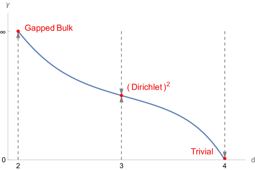
Figure 1: IR-stable fixed points in the free theory. The blue curve represents the fixed point dependence on the background theory dimension, and the grey dashed arrow indicates the RG flow from UV to IR. Fixed points with physical interpretations in integer dimensions are marked in red.

Lastly, we comment on an RG flow triggered by a $\gamma<0$ deformation. On the one hand, in this case equation (10) does not end at a finite fixed point. Instead, there exists a finite scale in which the 1-loop exactness of RG breaks down. On the other hand, we point out that the Hamiltonian is not bounded from below when $\gamma<0$ for a free background theory, and we expect that in this case there is a runaway behavior . However, for an interacting theory whose background potential is bounded from below, it could be the case where such a defect induces localized degrees of freedom and flows to a healthy DCFT in the IR. Such a setup will be studied in more detail in sections 3 and 4.

2.2 Defect Weyl Anomaly

In this subsection, we calculate the $b$-coefficient at the IR stable fixed point (11) and investigate its physics. Before the calculation, we notice that since the DCFT is still Gaussian and can be analyzed through Wick contraction, it falls into the category of a generalized free theory. The lowest-lying nontrivial defect operator $\hat{\phi}$ has the scaling dimension

$$\Delta(\hat{\phi})=1+\frac{\epsilon}{2},$$ (13)

at the stable IR fixed point (11). This bears similarities to double-trace deformations in a large-N two-dimensional CFT gubser2003universal , which motivates us to study the Weyl anomaly b-coefficient through the defect contribution to the free energy $\mathcal{F}$ jensen2016constraint ; shachar2022rg .

Consider the defect (3) of spherical geometry, that is, a $\mathbb{S}^{2}$ sphere of radius $R$ embedded in $\mathbb{R}^{d}$. The defect contribution to the free energy is defined by:

$$\mathcal{F}\equiv-\left(\log Z^{\text{DCFT}}-\log Z^{\text{CFT}}\right),$$ (14)

where $Z^{\text{DCFT}}$ is the partition function of the full theory with the presence of the defect, and $Z^{\text{CFT}}$ is that of the same background theory but without the defect. $\mathcal{F}$ generally depends on the regulation scheme and suffers from ambiguities. However, the $b$-coefficient, which can be extracted from the logarithmic IR-divergence of (14), is universal and scheme-independent jensen2016constraint ; shachar2022rg . In the $\mathbb{S}^{2}$ defect geometry, we have :

$$\mathcal{F}\sim a_{0}+a_{1}(\Lambda R)^{2}+\frac{b}{3}\log(\Lambda R),$$ (15)

where $a_{1}$ and $a_{0}$ are non-universal coefficients and $b$ satisfies the inequality $b_{\text{UV}}\geq b_{\text{IR}}$ at the UV and IR fixed points respectively jensen2016constraint ; shachar2022rg . Note that such a statement is for fixed point theories, and to avoid subtleties in the middle of the RG flow we will set the bare coupling to be at the stable IR fixed point (11) in the following, which reads:

$$(\gamma_{\text{b}})_{*}=2\pi\epsilon\Gamma(1-\frac{\epsilon}{2})\left(\frac{\Lambda}{2\sqrt{\pi}}\right)^{\epsilon}.$$ (16)

To derive $\mathcal{F}$, we will need to investigate the Laplacian operator eigenvalues in the presence of the defect. Due to the defect isometry group $SO(3)$, the Laplacian is diagonal in the momentum space dual to the $\mathbb{S}^{2}$ sphere coordinate. The free field propagator of spherical harmonic waves $\{\alpha_{l}\}$ (see equation (95) for definition) are given by:

$$\alpha_{l}(\epsilon)\equiv\frac{\left(\pi\epsilon/2\right)\Gamma\left(l-\frac{\epsilon}{2}+1\right)}{\sin\left(\pi\epsilon/2\right)\Gamma\left(l+\frac{\epsilon}{2}+1\right)}.$$ (17)

For a Gaussian theory as (3), $\mathcal{F}$ can be evaluated using basic linear algebra (see appendix A for details). It reads:

$$\mathcal{F}=\frac{1}{2}\sum_{l\geq 0}(2l+1)\log{\left(1+(\Lambda R)^{\epsilon}\alpha_{l}(\epsilon)\right)},$$ (18)

which diverges in the IR limit $R\rightarrow\infty$. To extract the IR information from the above expression we will apply a dimensional regulation scheme (similar to the analysis found in klebanov2011f ; diaz2007partition ) on the defect dimension $\tilde{d}$ (instead of the background space). In the IR limit, equation (18) can be simplified as follows (see e.g. diaz2007partition ):

$$\mathcal{F}=-\frac{1}{2}\sum_{l\geq 0}\text{deg}(\tilde{d},l)\log{\frac{\Gamma\left(l+\frac{\tilde{d}}{2}+\frac{\epsilon}{2}\right)}{\Gamma\left(l+\frac{\tilde{d}}{2}-\frac{\epsilon}{2}\right)}}\,,$$ (19)

where

$$\text{deg}(\tilde{d},l)\equiv(2l+\tilde{d}-1)\frac{\Gamma(l+\tilde{d}-1)}{\Gamma(l+1)\Gamma(\tilde{d})},$$ (20)

stands for the spherical harmonic degeneracy. In this regularization scheme, physical quantities are obtained by an analytic continuation to $\tilde{d}\rightarrow 2$. As in ordinary even dimensional CFTs, such a $\mathcal{F}$-function exhibits IR-divergence in $\tilde{\epsilon}\equiv\tilde{d}-2$. Thus, in this case, the pole in $O(1/\tilde{\epsilon})$ corresponds to the logtharmic IR-divergence in the cutoff regulation parameter (see e.g. graham1999volume ; diaz2007partition ), and shall be identified as the defect Weyl anomaly coefficient in equation (2). We find ($d\equiv 4-\epsilon$):

$$b_{\text{IR}}=-\frac{\epsilon^{3}}{8}.$$ (21)

The first consistency check is $b_{\text{IR}}<0$ when $d<4$. Note that at the UV fixed point of 10, the DCFT is trivial with $b_{\text{UV}}=0$. Hence indeed the inequality $b_{\text{UV}}\geq b_{\text{IR}}$ is satisfied in this example. The second check is when $\epsilon\ll 1$, (21) agrees with the perturbative result in shachar2022rg , and there are no higher order corrections. We comment that this is a consequence of the defect RG being 1-loop exact.

At $d=3$, the $b$-coefficient takes the value of two copies of the free field Dirichlet boundary condition ($b_{\text{D}}=-1/16$) jensen2016constraint . This observation is supported by the propagator at the fixed point $(\gamma_{b})_{*}=\pi\Lambda$:

$$\left[\delta_{p_{1}+p_{2}}(k^{2}+p_{1}^{2})+\pi\Lambda\right]^{-1}=\frac{\delta_{p_{1}+p_{2}}}{k^{2}+p_{1}^{2}}-\frac{2|k|}{(k^{2}+p_{1}^{2})(k^{2}+p_{2}^{2})}+O\left(\Lambda^{-3}\right).$$ (22)

where the subleading terms are suppressed by the cutoff $\Lambda$ and depend on the regulation scheme we chose. To see its physical meaning, we evaluate the layer susceptibility dey2020operator ; shpot2021boundary

$$\chi(y_{1},y_{2}):= \lim_{|k|\rightarrow 0}\int\frac{dp_{1}}{2\pi}\frac{dp_{2}}{2\pi}e^{i(p_{1}y_{1}+p_{2}y_{2})}\left(\frac{\delta_{p_{1}+p_{2}}}{k^{2}+p_{1}^{2}}-\frac{2|k|}{(k^{2}+p_{1}^{2})(k^{2}+p_{2}^{2})}\right)$$ (23)

$$= \lim_{|k|\rightarrow 0}\left(\frac{e^{-|k||y_{1}-y_{2}|}}{2|k|}-\frac{e^{-|k|(|y_{1}|+|y_{2}|)}}{2|k|}\right)$$

$$= \frac{1}{2}(|y_{1}|+|y_{2}|-|y_{1}-y_{2}|).$$

such that if $y_{1}$ and $y_{2}$ are on different sides of the plane defect, the susceptibility vanishes in the IR. In this case, the presence of the defect simply breaks space into two. That is, the theory in $\mathbb{R}^{3}$ at IR is broken into two distinct copies of free scalar in half-spaces $\mathbb{R}^{3}_{+}$ with Dirichlet boundary conditions, which agrees with the result (21) for the $b$-coefficient.

At $d=2$, there is a subtlety since one can no longer perform the Weyl transformation individually to the defect, as it is now indistinguishable from the background theory. It is known that a 2d free scalar (should be thought of as the large radius limit of a compact boson) has a central charge $c=1$ ginsparg1988applied . Therefore, the physical Weyl anomaly coefficient is $b_{\text{IR}}+c=0$. We note this agrees with equation (10) and the phase diagram 1, such that the fixed point is a two-dimensional gapped trivial theory.

3 The $O(N)$ Wilson-Fisher Fixed Point

In this section, we study the analog of (4) with the background theory being the $O(N)$ interacting model tuned to the Wilson-Fisher fixed point wilson1974renormalization in $d=4-\epsilon$ dimension. Throughout this section, we will assume that $\epsilon\ll 1$ is the smallest parameter in the theory and that the defect couplings are of the order $O(\epsilon)$ such that standard perturbation theory is valid.

The background theory can be described by $N$ scalar fields $\{\phi^{i}\}$ with $1\leq i\leq N$ coupled through $\phi^{4}$-interactions in flat space $\mathbb{R}^{d}$. We will denote the interactions by a fully symmetric (dimensionless) coupling tensor $\{\lambda_{ijkl}\}$, such that:

$$S_{0}=\int_{\mathbb{R}^{d}}d^{d}x\left\{\frac{1}{2}(\partial\phi^{i})^{2}+\frac{\Lambda^{4-d}}{4!}\lambda_{ijkl}\phi^{i}\phi^{j}\phi^{k}\phi^{l}\right\},$$ (24)

where $\Lambda$ is the UV scale. The interacting RG fixed point of our interest to its 1-loop level value is given by wilson1974renormalization :

$$(\lambda_{ijkl})_{*} =\frac{16\pi^{2}\epsilon}{N+8}(\delta_{ij}\delta_{kl}+\delta_{ik}\delta_{jl}+\delta_{il}\delta_{jk})+O\left(\epsilon^{2}\right).$$ (25)

An implicit assumption in the following discussion is locality: in the defect’s presence, we will continue to work in the background fixed point defined by (25). We will use the same coordinate system as in the last section, such that $x=(y,z)$. When an operator is inserted at $(y,0)$ or $(0,z)$ we will abuse the notation to denote them as $(z)$ and $(y)$, correspondingly. Defect perturbations to the background theory considered in this section can be roughly summarized as $\phi$-quadric operators being inserted at the $y=0$ plane, such that the flip symmetry $\mathbb{Z}_{2}:\phi^{i}\rightarrow-\phi^{i}$ is always preserved.

In the following, we first review in subsection 3.1 the conformal data of the background theory that will be used in the defect analysis. In subsection 3.2 we perform the perturbative analysis in the theory with defect insertion and obtain the $O(N)$-DCFT fixed points. Last, in subsection 3.3 we analyze in greater detail the fixed point structure upon explicit forms of $O(N)$ breaking deformations that appear in the one-loop level.

3.1 Background Data

At the background fixed point (25), conformally well-defined $\phi$-quadratic operators are packed in irreducible representations of $O(N)$. The lowest-lying $O(N)$-singlet and $O(N)$-symmetric traceless operators are given by kehrein1995spectrum ; henriksson2023critical :

$$\mathcal{O}(x)= \frac{1}{2N}\left[\sum_{1\leq k\leq N}(\phi^{k})^{2}\right](x)\,,$$ (26)

$$T^{ij}(x)= \left[\phi^{i}\phi^{j}-\frac{\delta_{ij}}{N}\sum_{1\leq k\leq N}(\phi^{k})^{2}\right](x)\,.$$ (27)

The two-point functions read cuomo2022localized :

$$\langle\mathcal{O}(x_{1})\mathcal{O}(x_{2})\rangle= \frac{\mathcal{N}_{\mathcal{O}}^{2}}{|x_{1}-x_{2}|^{2\Delta_{\mathcal{O}}}}\,,$$ (28)

$$\langle T^{ij}(x_{1})T^{kl}(x_{2})\rangle= \left(\delta^{ik}\delta^{jl}+\delta^{il}\delta^{jk}-\frac{2}{N}\delta^{ij}\delta^{kl}\right)\frac{\mathcal{N}_{T}^{2}}{|x_{1}-x_{2}|^{2\Delta_{T}}}.$$ (29)

where:

$$\Delta_{\mathcal{O}}=2-\frac{6}{N+8}\epsilon+O\left(\epsilon^{2}\right);\quad\mathcal{N}_{\mathcal{O}}=\frac{1}{4\pi^{2}\sqrt{2N}}+O\left(\epsilon\right)\,,$$ (30)

$$\Delta_{T}=2-\frac{N+6}{N+8}\epsilon+O\left(\epsilon^{2}\right);\quad\mathcal{N}_{T}=\frac{1}{4\pi^{2}}+O\left(\epsilon\right)\,.$$ (31)

In what follows, we will also need the three-point correlation functions involving these operators, for which we take the convention

$$\langle\mathcal{O}_{a}(x_{1})\mathcal{O}_{b}(x_{2})\mathcal{O}_{c}(x_{3})\rangle =\frac{C_{\mathcal{O}_{a}\mathcal{O}_{b}\mathcal{O}_{c}}}{|x_{1}-x_{2}|^{\Delta_{a}+\Delta_{b}-\Delta_{c}}|x_{2}-x_{3}|^{\Delta_{b}+\Delta_{c}-\Delta_{a}}|x_{3}-x_{1}|^{\Delta_{c}+\Delta_{a}-\Delta_{b}}}\,,$$ (32)

where $\mathcal{O}_{a}=\{\mathcal{O}(x),T^{ij}(x)\}$. The OPE coefficients $C_{\mathcal{O}_{a}\mathcal{O}_{b}\mathcal{O}_{c}}$ can be perturbatively calculated, and to their leading order in $O(\epsilon^{0})$ it yields:

$$C_{\mathcal{O}\mathcal{O}\mathcal{O}} =\frac{1}{64N^{2}\pi^{6}}\,,$$ (33)

$$C_{\mathcal{O}\mathcal{O}T^{ij}} =0\,,$$ (34)

$$C_{\mathcal{O}T^{ij}T^{kl}} =\frac{1}{32N\pi^{6}}\left(\delta^{ik}\delta^{jl}+\delta^{il}\delta^{jk}-\frac{2}{N}\delta^{ij}\delta^{kl}\right)\,,$$ (35)

$$C_{T^{ij}T^{kl}T^{mn}} =\frac{1}{64\pi^{6}}\left(\delta^{ik}\delta^{ln}\delta^{mj}+\delta^{jk}\delta^{ln}\delta^{mi}+\delta^{il}\delta^{kn}\delta^{mj}+\delta^{ik}\delta^{lm}\delta^{nj}\right.$$ (36)

$$+ \delta^{jl}\delta^{km}\delta^{ni}+\delta^{il}\delta^{km}\delta^{nj}+\delta^{jk}\delta^{lm}\delta^{ni}+\delta^{jl}\delta^{kn}\delta^{mi}-\frac{4\delta^{ij}}{N}(\delta^{mk}\delta^{nl}+\delta^{nk}\delta^{ml})$$

$$- \frac{4\delta^{kl}}{N}(\delta^{im}\delta^{jn}+\delta^{in}\delta^{jm})\left.-\frac{4\delta^{mn}}{N}(\delta^{ik}\delta^{jl}+\delta^{il}\delta^{jk})+\frac{16}{N^{2}}\delta^{ij}\delta^{kl}\delta^{mn}\right).$$

3.2 Defect RG Flow

In analogy with equation (4), the defect is parametrized by a scalar $\gamma$ and a tensor $g_{ij}$ dimensionless coupling, such that the action is given by:

$$S=S_{0}+\int_{\mathbb{R}^{2}}d^{2}z\Lambda^{2}\left\{\frac{\gamma}{\Lambda^{\Delta_{\mathcal{O}}}}\mathcal{O}+\frac{g_{ij}}{\Lambda^{\Delta_{T}}}T^{ij}\right\}\,,$$ (37)

where $S_{0}$ is given by equation (24), and the background theory is considered at Wilson-Fisher fixed point (25). As mentioned previously in this section, perturbative analysis can be performed by assuming $\{\gamma,g_{ij}\}\sim O(\epsilon)$. In the framework of conformal perturbation theory komargodski2017random , the one-point function of the singlet operator $\mathcal{O}$ takes the following form:

$$\langle\mathcal{O}(y)\rangle= -\Lambda^{\frac{6\epsilon}{N+8}}\gamma\int d^{2}z\langle\mathcal{O}(y)\mathcal{O}(z)\rangle+\Lambda^{\frac{12\epsilon}{N+8}}\frac{\gamma^{2}}{2}\int d^{2}z_{1}d^{2}z_{2}\langle\mathcal{O}(y)\mathcal{O}(z_{1})\mathcal{O}(z_{2})\rangle$$ (38)

$$+\Lambda^{2\frac{N+6}{N+8}\epsilon}\frac{g_{ij}g_{kl}}{2}\int d^{2}z_{1}d^{2}z_{2}\langle\mathcal{O}(y)T^{ij}(z_{1})T^{kl}(z_{2})\rangle+O\left(\epsilon^{3}\right)$$

$$= -\frac{1}{32\pi^{3}N|y|^{\Delta_{\mathcal{O}}}}\left(\gamma-\frac{N+8}{12\pi N\epsilon}\gamma^{2}-\frac{(N+8)}{\pi(N+3)\epsilon}\text{Tr}\{g^{2}\}+O\left(\epsilon^{2}\right)\right).$$

Using the minimal subtraction scheme (MS, see appendix B for details) one obtains the following (minus-)beta function

$$-\beta(\gamma)=\frac{6\epsilon}{N+8}\gamma-\frac{\gamma^{2}}{2\pi N}-\frac{2}{\pi}\text{Tr}\{g^{2}\}+O\left(\epsilon^{3}\right)\,.$$ (39)

Another useful observable is the one-point function of the traceless symmetric operator $T^{ij}$, which reads:

$$\langle T^{ij}(y)\rangle= -\Lambda^{\frac{N+6}{N+8}\epsilon}g_{kl}\int d^{2}z\langle T^{ij}(y)T^{kl}(z)\rangle$$ (40)

$$+\Lambda^{\frac{N+12}{N+8}\epsilon}\gamma g_{kl}\int d^{2}z_{1}d^{2}z_{2}\langle T^{ij}(y)\mathcal{O}(z_{1})T^{kl}(z_{2})\rangle$$

$$+\Lambda^{2\frac{N+6}{N+8}\epsilon}\frac{g_{kl}g_{mn}}{2}\int d^{2}z_{1}d^{2}z_{2}\langle T^{ij}(y)T^{kl}(z_{1})T^{mn}(z_{2})\rangle+O\left(\epsilon^{3}\right)$$

$$= -\frac{1}{8\pi^{3}|y|^{\Delta_{T}}}\left(g_{ij}-\frac{N+8}{6\pi N\epsilon}g_{ij}\gamma-\frac{N+8}{\pi(N+6)\epsilon}\left((g^{2})_{ij}-\frac{\delta_{ij}}{N}\text{Tr}\{g^{2}\}\right)\right)\,.$$

Using the MS scheme we find:

$$-\beta(g_{ij})= \frac{N+6}{N+8}\epsilon g_{ij}-\frac{g_{ij}\gamma}{\pi N}-\frac{1}{\pi}\left((g^{2})_{ij}-\frac{\delta_{ij}}{N}\text{Tr}\{g^{2}\}\right)+O\left(\epsilon^{3}\right).$$ (41)

In the following, we are to investigate the solutions of null beta functions (39) and (41) at the vicinity of the trivial fixed point, such that they are continuously connected to $\gamma=g_{ij}=0$ at the limit $\epsilon\to 0$.

Obviously, for all $N$ there exists a $O(N)$-symmetric fixed point:

$$\gamma=\gamma_{*}\equiv\frac{12\pi N}{N+8}\epsilon+O\left(\epsilon^{2}\right);\quad g_{ij}=0,$$ (42)

which is IR-stable against $O(N)$ symmetric deformation. In $O(N)$ preserving cases, while the flow triggered by a $\gamma>0$ deformation ends in the stable fixed point (42), a $\gamma<0$ one from (39) naively implies a flow toward minus infinity. However, of course, this exceeds the perturbative regime and the end point of such a flow is beyond the scope of this section. One possibility for the physical behavior in this regime arises from the EFT description proposed in section 4.

The lowest-lying defect primaries at the fixed point (42) include

$$\Delta(\hat{\phi}^{i})= 1-\frac{N+20}{2N+16}\epsilon+O\left(\epsilon^{2}\right),$$ (43)

$$\Delta(\hat{T}^{ij})= 2-\frac{N-6}{N+8}\epsilon+O\left(\epsilon^{2}\right).$$

The defect order parameters $\{\hat{\phi}^{i}\}$, not surprisingly, are relevant when $\epsilon\ll 1$. However, for $\{T^{ij}\}$ deformations, the statement will depend on $N$: when $N<6$ the fixed point in (42) is stable, while when $N>6$ it is unstable. When $N=6$, the one-loop analysis result (41) suggests that the stability depends on the specific deformations that are being triggered. We elaborate on these cases and classify the various deformations in the following subsection 3.3.

Another notable statement is that there exists a single operator, which is $O(N)$-singlet, of $\mathbb{S}^{1-\epsilon}$ spin 1 and protected dimension 3. This is the displacement operator, and we will denote it as $\partial_{y}\hat{\mathcal{O}}$ to illustrate that it is continuously connected to the $\mathcal{O}$ level-1 descendant along the RG flow.

Finally, as a counterpart to the free theory discussion (21), we present the defect Weyl anomaly. The perturbative result is extensively studied in shachar2022rg , and following the results derived therein, together with the fixed point (42), we find:

$$b_{\text{IR}}=-(2-\Delta_{\mathcal{O}})(\pi\mathcal{N}_{\mathcal{O}}\gamma_{*})^{2}+O\left(\epsilon^{4}\right)=-\frac{27N}{(N+8)^{3}}\epsilon^{3}+O\left(\epsilon^{4}\right).$$ (44)

3.3 Perturbative Fixed Points

Following the discussion in the last subsection, we move on to study perturbative fixed points of maximal symmetries that can be preserved by $\{T^{ij}\}$, that is $O(M)\times O(N-M)\subseteq O(N)$. Since beta functions (39) and (41) are quadratic in couplings at the one-loop level, we note this is the only symmetry pattern that can be found from solving null conditions to leading perturbative order. However, in principle, one could calculate higher-loop corrections and obtain a more complicated symmetry group.

We consider the following deformation, being triggered along with $\mathcal{O}$ as in equation (37):

$$g_{ij}T^{ij}=g_{M}\left[-\frac{1}{M}\sum_{i\leq M}(\phi^{i})^{2}+\frac{1}{N-M}\sum_{i>M}(\phi^{i})^{2}\right],$$ (45)

for $1\leq M<N$ and with the convention $g_{M}>0$. The beta function (41) for $g_{M}$ reduces to:

$$-\beta(g_{M})=\frac{N+6}{N+8}\epsilon g_{M}-\frac{g_{M}\gamma}{\pi N}-\frac{2M-N}{\pi M(N-M)}g_{M}^{2}+O\left(\epsilon^{3}\right).$$ (46)

In what follows, we classify the fixed-point solutions according to cases of $\{M,N\}$.

When $N<6$, each choice of $M$ admits a single solution to null equations of (39) and (41). In the space spanned by $\gamma$ and $g_{M}$, such fixed points have one relevant direction and therefore they are unstable.

When $N=6$, at the fixed point (42) we have the beta function (46)

$$\left.-\beta(g_{M})\right|_{\gamma=\gamma_{*},N=6}=\frac{M-3}{M-6}\frac{2g^{2}_{M}}{\pi M}+O\left(\epsilon^{3}\right),$$ (47)

such that for $M>3$ the operator $\hat{T}_{M}$ is irrelevant, and one meta-stable fixed point can be found, similarly to the cases of $N<6$. For $M=3$, the meta-stable fixed point collides with the $O(N)$-symmetric one of equation (42) at the one-loop level, and the solution is sensitive to higher-loop corrections. For $M<3$, on the other hand, null equations of (39) and (41) yield no finite positive solution to $g_{M}$. We note in these cases $\hat{T}_{M}$ at the fixed-point (42) is relevant, and the RG being triggered flows toward large couplings, where the perturbative scheme breaks down. We will therefore categorize $\{M>3,N=6\}$ cases as in the same class of $N<6$, where the single $O(M)\times O(N-M)$ fixed point is unstable to one deformation, and present the data in table 1.

$((g_{M})_{*},\gamma_{*})$	$N=2$	$N=3$	$N=4$	$N=5$	$N=6$
$M=1$	$\left(\frac{\sqrt{2}}{5},\frac{8}{5}\right)$	$\left(\frac{4\sqrt{7}-2}{33},\frac{26+2\sqrt{7}}{11}\right)$	$\left(\frac{\sqrt{6}-1}{8},\frac{9+\sqrt{6}}{3}\right)$	$\left(\frac{8\sqrt{5}-12}{65},\frac{46+6\sqrt{5}}{13}\right)$	No FP
$M=2$		$\left(\frac{4\sqrt{7}+2}{33},\frac{26-2\sqrt{7}}{11}\right)$	$\left(\frac{\sqrt{5}}{6},\frac{10}{3}\right)$	$\left(\frac{12\sqrt{3}-6}{65},\frac{54+2\sqrt{3}}{13}\right)$	No FP
$M=3$			$\left(\frac{\sqrt{6}+1}{8},\frac{9-\sqrt{6}}{3}\right)$	$\left(\frac{12\sqrt{3}+6}{65},\frac{54-2\sqrt{3}}{13}\right)$	?
$M=4$				$\left(\frac{8\sqrt{5}+12}{65},\frac{46-6\sqrt{5}}{13}\right)$	$\left(\frac{8}{21},\frac{32}{7}\right)$
$M=5$					$\left(\frac{10}{21},\frac{20}{7}\right)$

Table 1: Fixed points for $N\leq 6$ (in addition to the trivial and $O(N)$ symmetric ones).The couplings are in units of $\pi\epsilon$ and only the leading orders are presented. At $N=6$ and $M=3$, the fixed point existence needs to be discussed at a higher-loop level.

When $N>6$, most choices of $\{M,N\}$ admit no perturbative fixed point other than the trivial one and the $O(N)$-symmetric one (42), similar to $\{M<3,N=6\}$. Exceptions exist for $\{M=N-1,6<N<10\}$, where there are two $O(N-1)\times\mathbb{Z}_{2}$ fixed points. We will denote the unstable one as FP-1 and the stable one as FP-2. When $N=10$, FP-1 and FP-2 collide at the 1-loop level, and higher loop corrections are needed to specify the existence and number of the fixed point. Data corresponding to the aforementioned cases are presented in table 2.

$((g_{M})_{*},\gamma_{*})$	$N=7$	$N=8$	$N=9$	$N=10$
FP-1	$\left(\frac{10+4\sqrt{3}}{35},\frac{66-10\sqrt{3}}{15}\right)$	$\left(\frac{21+7\sqrt{2}}{64},\frac{19-3\sqrt{2}}{4}\right)$	$\left(\frac{8}{17},\frac{72}{17}\right)$	?
FP-2	$\left(\frac{10-4\sqrt{3}}{35},\frac{66+10\sqrt{3}}{15}\right)$	$\left(\frac{21-7\sqrt{2}}{64},\frac{19+3\sqrt{2}}{4}\right)$	$\left(\frac{40}{153},\frac{100}{17}\right)$	?

Table 2: Fixed points for $\{M=N-1,6<N\leq 10\}$ (in addition to the trivial and $O(N)$ symmetric ones). The couplings are in units of $\pi\epsilon$ and only the leading orders are presented. At $\{M=9,N=10\}$, FP-1 and FP-2 collide at the 1-loop level and higher loops are needed to distinguish them.

To conclude this part, we have obtained the perturbative phase diagram (see figure 2 for an illustration of cases) and the one-loop perturbative fixed points within. It is a physically interesting question to ask what is the IR theory at the end of the asymptotic directions described above. This will be further studied in the next section.

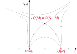
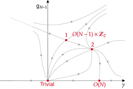
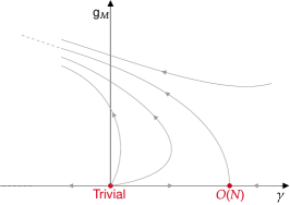
Figure 2: The perturbative phase diagram for $O(M)\times O(N-M)$ defects. Left: cases listed in table 1. Middle: cases listed in table 2. Right: cases of no fixed point other than the trivial one and $O(N)$-symmetric one.

4 Effective Action and Phase Diagram

In the following, we discuss possible effective actions of the non-perturbative fixed points mentioned in the last section and propose completion of the phase diagram from figure 2. Classically, since $g_{M}$ and $-\gamma$ flow to large values as suggested by (39) and (41), the defect has a tendency to acquire localized degrees of freedom. Inspired by similar studies krishnan2023plane ; metlitski2022boundary , we make the assumption that the effective actions consist of three parts:

• A DCFT of the background theory $S_{\mathcal{D}}$.

• An action associated with the localized defect degrees of freedom $S_{\sigma}$.

• Couplings between the two theories $S_{\mathcal{D}}$ and $S_{\sigma}$.

We will further assume that $S_{\sigma}$ can be described by the two-dimensional Non-Linear Sigma Model (NL$\Sigma$M) zinn2021quantum ; henriksson2023critical . This follows from the consideration that symmetry patterns as discussed in the previous section are $O(M)\times O(N-M)$, among which classically a $O(M)$ order parameter is favored by a large coupling $g_{M}$. Consistency check and verification of such an effective action proposal will be the main subject of this section.

For simplicity, we will use a coordinate system slightly different from previous ones throughout this section. Let $y\in\mathbb{R}^{+}$ be the distance to the defect and $\Omega^{d-3}\in\mathbb{S}^{d-3}$ be the compact notation of the spherical coordinates, such that $x=(y,\Omega^{d-3},z)$. We remind readers that the background theory is the same as in section 3: the $O(N)$ Wilson-Fisher fixed point at $\epsilon\equiv 4-d\ll 1$. The fact that the background theory, contrary to the defect theory, is perturbative will be essential in our following analysis.

This section is organized as follows. In subsection 4.1, we identify the saddle point of $S_{\mathcal{D}}$ and perform a perturbative analysis around it. In subsection 4.2, we extract DFCT data of our interest from $S_{\mathcal{D}}$. Finally, in subsection 4.3, we show that the coupling between $S_{\mathcal{D}}$ and $S_{\sigma}$ is unique and verify the NL$\Sigma$M stability.

4.1 Mean Field and $\mathbb{H}^{3}\times\mathbb{S}^{d-3}$

We will take $S_{\mathcal{D}}$ to be the surface analog of the line defect induced by a localized magnetic field in $O(N)$ Wilson-Fisher fixed point Cuomo:2021rkm , where the background order parameter $\phi^{i}$ acquires a non-zero vacuum expectation value when being evaluated close to the defect. We note that similar problems were also studied in the context of the boundary universality class burkhardt1987surface ; mcavity1995conformal ; shpot2021boundary ; dey2020operator ; Padayasi:2021sik . For our purpose, we will study the perturbative expansion around the mean-field profile. The profile is subject to the classical equation of motion, which reads:

$$\left(-\partial^{2}_{\mathbb{R}^{d}}+\frac{\lambda_{\text{b}}}{6}\left(\phi_{\text{cl}}(x)\right)^{2}\right)\phi_{\text{cl}}(x)=0\,.$$ (48)

In addition to the trivial solution $\phi_{\text{cl}}(x)=0$, equation (48) admits a profile that is singular when evaluated close to the defect at $y=0$:

$$\phi_{\text{cl}}(x)=\sqrt{\frac{6(1+\epsilon)}{\lambda_{\text{b}}}}\frac{1}{y}\,.$$ (49)

We then facilitate a field redefinition and study the fluctuations on top of the configuration (49). Explicitly, we define the fluctuation fields $\{\tilde{\phi}^{i}\}$ according to:

$$\phi^{i}(x)=\delta^{i1}\phi_{\text{cl}}(x)+\tilde{\phi}^{i}(x).$$ (50)

The action of the background fields (24) can be recasted into the classical part and a functional of the fluctuation fields, which reads:

$$S_{0}= \int_{y>\frac{1}{\Lambda}}d^{d}x\left\{\frac{1}{2}(\partial\phi^{i})^{2}+\frac{\lambda_{\text{b}}}{4!}[(\phi^{i})^{2}]^{2}\right\}$$ (51)

$$= S_{\text{cl}}+\int_{y>\frac{1}{\Lambda}}d^{d}x\left\{\frac{1}{2}(\partial\tilde{\phi}^{i})^{2}+\frac{1+\epsilon}{2y^{2}}\left[(\tilde{\phi}^{i})^{2}+2(\tilde{\phi}^{1})^{2}\right]\right.$$

$$\left.+\sqrt{\frac{(1+\epsilon)\lambda_{\text{b}}}{6}}\frac{\tilde{\phi}^{1}}{y}(\tilde{\phi}^{i})^{2}+\frac{\lambda_{\text{b}}}{4!}\left[(\tilde{\phi}^{i})^{2}\right]^{2}\right\}.$$

In order to perform perturbative analysis with respect to the coupling $\lambda_{\text{b}}$, it is useful to compute the saddle point propagator. We digress here to discuss generally how this can be obtained. Consider the Green’s function $G(x,{x}^{\prime})$ subject to the following equation:

$$\left(-\partial^{2}_{\mathbb{R}^{d}}+\frac{(6-d)(d-2)+4m^{2}}{4y^{2}}\right)G(x,{x}^{\prime})=\delta_{\mathbb{R}^{d}}(x-{x}^{\prime}).$$ (52)

with $m^{2}\in\mathbb{R}$ being a constant. This problem can be effectively solved by a Weyl transformation from $\mathbb{R}^{d}$ to $\mathbb{H}^{3}\times\mathbb{S}^{d-3}$ (see e.g. nishioka2021free ; Cuomo:2021rkm ):

$$d^{2}s= d^{2}z+d^{2}y+y^{2}d^{2}\Omega^{d-3}$$ (53)

$$= y^{2}\left(\frac{d^{2}z+d^{2}y}{y^{2}}+d^{2}\Omega^{d-3}\right)$$

$$= y^{2}d^{2}\tilde{s}\rightarrow d^{2}\tilde{s}\,.$$

We will denote the Weyl transformation of $G(x,{x}^{\prime})$ as $\tilde{G}(x,{x}^{\prime})$. One finds:

$$(-\partial^{2}_{\mathbb{H}^{3}}-\partial^{2}_{\mathbb{S}^{1-\epsilon}}+m^{2})\tilde{G}(x,{x}^{\prime})=\delta_{\mathbb{H}^{3}\times\mathbb{S}^{1-\epsilon}}(x-{x}^{\prime}).$$ (54)

where $m^{2}$ has a physical interpretation of mass term in $\mathbb{H}^{3}\times\mathbb{S}^{d-3}$. To solve the above, we can first perform an expansion by $\mathbb{S}^{1-\epsilon}$ spherical harmonics $Y_{l,q}(\Omega)$:

$$\tilde{G}(x,{x}^{\prime})=\sum_{l\geq 0,q}Y_{l,q}(\Omega)Y^{*}_{l,q}({\Omega}^{\prime})\tilde{G}(\xi;l)\,,$$ (55)

where

$$-\partial^{2}_{\mathbb{S}^{1-\epsilon}}Y_{l,q}(\Omega)= l(l-\epsilon)Y_{l,q}(\Omega),$$ (56)

$$\sum_{q}1= \text{deg}(1-\epsilon,l),$$

and the degeneracy is given by equation (20). In the above, the dependence on the variable $\xi$ is fixed by the $\mathbb{H}^{3}$ isometry:

$$\xi=\frac{2y{y}^{\prime}}{y^{2}+{y}^{\prime 2}+(z-{z}^{\prime})^{2}}.$$ (57)

The solution for each $\mathbb{S}^{1-\epsilon}$ spin $l$ functions $\tilde{G}(\xi;l)$ is given by the standard Euclidean $AdS_{3}$ bulk to bulk propagator, which has been well studied d2004supersymmetric , and reads:

$$\tilde{G}(\xi;l)= \frac{1}{2\pi}\left(\frac{\xi}{2}\right)^{\Delta_{l}}\,_{2}F_{1}\left(\frac{\Delta_{l}}{2},\frac{\Delta_{l}+1}{2};\Delta_{l};\xi^{2}\right),$$ (58)

where $\Delta_{l}$ are given by $\Delta_{l}\equiv 1+\sqrt{1+m^{2}+l(l-\epsilon)}$. These correspond to the (non-singular at the $\xi\to 0$ limit) solution to the conformal boundary condition, as follows from the analysis in nishioka2021free .

Notice that since the defect breaks the Poincare symmetry and introduces a scale $y$, the Green function in this case acquires a non-zero value at the coincident point after regulation. Let $\text{vol}(\mathbb{S}^{1-\epsilon})$ be the volume of the unit sphere $\mathbb{S}^{1-\epsilon}$, one finds:

$$\tilde{G}(x,x)= \sum_{l\geq 0}\frac{\deg(1-\epsilon,l)}{\text{vol}(\mathbb{S}^{1-\epsilon})}\lim_{\xi\rightarrow 1}\tilde{G}(\xi;l)$$ (59)

$$= \sum_{l\geq 0}\frac{\deg(1-\epsilon,l)}{\text{vol}(\mathbb{S}^{1-\epsilon})}\lim_{\xi\rightarrow 1}\left(\frac{i}{4\sqrt{2}\pi\sqrt{\xi-1}}+\frac{1-\Delta_{l}}{4\pi}+O\left(\sqrt{\xi-1}\right)\right)$$

$$= -\sum_{l\geq 0}\frac{\deg(1-\epsilon,l)}{4\pi\text{vol}(\mathbb{S}^{1-\epsilon})}\sqrt{1+m^{2}+l(l-\epsilon)},$$

where in the last equation, we have used the fact that $\sum_{l\geq 0}\deg(1-\epsilon,l)=0$ under dimensional regulation. To solve the above expression to its leading order, we apply a method similar to that in cuomo2022localized and expand summation terms around $l=\infty$

$$\tilde{G}(x,x)= -\frac{\pi^{\frac{\epsilon}{2}}\Gamma\left(1-\frac{\epsilon}{2}\right)}{8\pi^{2}}+\sum_{l\geq 1}\left(-\frac{2^{\epsilon}\pi^{\frac{\epsilon-1}{2}}l^{1-\epsilon}}{4\pi\Gamma\left(\frac{1}{2}-\frac{\epsilon}{2}\right)}-\frac{2^{\epsilon-3}\pi^{\frac{\epsilon-3}{2}}(\epsilon-1)\epsilon l^{-\epsilon}}{\Gamma\left(\frac{1}{2}-\frac{\epsilon}{2}\right)}\right.$$ (60)

$$\left.-\frac{2^{\epsilon-5}\pi^{\frac{\epsilon-3}{2}}\left(3\epsilon^{4}-2\epsilon^{3}+2\epsilon+12+12m^{2}\right)l^{-1-\epsilon}}{3\Gamma\left(\frac{1}{2}-\frac{\epsilon}{2}\right)}+O\left(l^{-2-\epsilon}\right)\right)$$

$$= -\frac{2^{\epsilon-5}\pi^{\frac{\epsilon-3}{2}}\left(3\epsilon^{4}-2\epsilon^{3}+2\epsilon+12+12m^{2}\right)}{3\Gamma\left(\frac{1}{2}-\frac{\epsilon}{2}\right)}\zeta(\epsilon+1)+O\left(\epsilon^{0}\right)$$

$$= -\frac{1+m^{2}}{8\pi^{2}\epsilon}+O\left(\epsilon^{0}\right)\,.$$

In the above, between the first and second equations we have used dimensional regularization to replace the summation in $l$ with a summation over Riemann zeta functions. Going from the second to the third equations, we notice that the zeta function has a single simple pole at $1$. Under an expansion in $\epsilon\ll 1$, the leading contribution will be from the $\zeta(\epsilon+1)$ term in the summation.

Finally, we perform the inverse Weyl transformation to obtain Green’s function of the original theory in flat space with a plane defect, which reads:

$$G(x,{x}^{\prime})= \frac{\tilde{G}(x,{x}^{\prime})}{(y{y}^{\prime})^{d/2-1}}.$$ (61)

Comparing equation (52) with the mean-field saddle point action (51), for the longitudinal (L) mode $\tilde{\phi}^{1}$ and transversal (T) modes $\tilde{\phi}^{i\geq 2}$ we correspondingly find:

$$m_{\text{L}}^{2}= 2+3\epsilon+\frac{\epsilon^{2}}{4},$$ (62)

$$m_{\text{T}}^{2}= \epsilon+\frac{\epsilon^{2}}{4}.$$

The associated Green’s function will be denoted by $G_{\text{L}/\text{T}}(x,{x}^{\prime})$ respectively. The DCFT $S_{\mathcal{D}}$ of interest has the following one-point expectation value:

$$\langle\phi^{i}(x)\rangle= \delta^{i1}\frac{a_{\sigma}}{y^{\Delta_{\phi}}}\,,$$ (63)

where the scaling dimension is given by kehrein1995spectrum ; henriksson2023critical :

$$\Delta_{\phi}= 1-\frac{\epsilon}{2}+O\left(\epsilon^{2}\right).$$ (64)

In the following, we illustrate how this is manifested by the mean-field analysis to the 1-loop level. Consider the formal expansion of $\langle\phi^{1}(x)\rangle$ as (see figure 3):

$$\langle\phi^{1}(x)\rangle= \phi_{\text{cl}}(x)-\frac{\lambda_{\text{b}}}{2}\int d^{d}{x}^{\prime}G_{\text{L}}(x,{x}^{\prime})G_{\text{L}}({x}^{\prime},{x}^{\prime})\phi_{\text{cl}}({x}^{\prime})$$ (65)

$$-\frac{N-1}{6}\lambda_{\text{b}}\int d^{d}{x}^{\prime}G_{\text{L}}(x,{x}^{\prime})G_{\text{T}}({x}^{\prime},{x}^{\prime})\phi_{\text{cl}}({x}^{\prime})+O\left(\lambda_{\text{b}}^{3/2}\right)$$

$$= \sqrt{\frac{6(1+\epsilon)}{\lambda_{\text{b}}}}\frac{1}{y}+\sqrt{\frac{(1+\epsilon)\lambda_{\text{b}}}{6}}\frac{1}{y^{1-\epsilon}}\left[\frac{N+8}{16\pi^{2}\epsilon}+O\left(\epsilon^{0}\right)\right]+O\left(\lambda_{\text{b}}^{3/2}\right),$$

where the bare coupling $\lambda_{\text{b}}$ in terms of the cut-off $\Lambda$ and renormalzied coupling $\lambda$ reads:

$$\lambda_{\text{b}}=\Lambda^{\epsilon}\left(\lambda+\frac{N+8}{48\pi^{2}\epsilon}\lambda^{2}+O\left(\lambda^{3}\right)\right).$$ (66)

Figure 3: One-loop Feynman diagrams that contribute to equation (65). Dashed lines represent the mean-field profile (49), and solid lines represent the Green’s function $G_{\text{L}/\text{T}}(x,{x}^{\prime})$.

From the above we find that indeed the pole term in (65) cancels, in agreement with the regulation scheme in (60) and the perturbative analysis:

$$\langle\phi^{1}(x)\rangle=\sqrt{\frac{6(1+\epsilon)}{\lambda}}\frac{1}{\Lambda^{\epsilon/2}y}+\sqrt{\frac{\lambda}{6}}\left[\frac{N+8}{16\pi^{2}}\log\left(y\Lambda\right)+O\left(\epsilon\right)\right]+O\left(\lambda^{3/2}\right).$$ (67)

Finally, plugging the fixed point value kehrein1995spectrum ; henriksson2023critical :

$$\lambda=\lambda_{*}=\frac{48\pi^{2}\epsilon}{N+8}\left(1+\frac{3(3N+14)}{(N+8)^{2}}\epsilon+O\left(\epsilon^{2}\right)\right)\,,$$ (68)

We find $\langle\phi^{1}(x)\rangle$ to the leading order in $\epsilon$ has the expected scaling dimension as in equation (63), and $a_{\sigma}$ reads:

$$a_{\sigma}=\frac{1}{2\pi}\sqrt{\frac{N+8}{2\epsilon}}\left[1+\frac{N^{2}+7N+22}{2(N+8)^{2}}\epsilon+O\left(\epsilon^{2}\right)\right].$$ (69)

4.2 DCFT Data

As locality requires, the assumed couplings between $S_{\sigma}$ and $S_{\mathcal{D}}$ should be between defect degrees of freedom and those of the neighboring background layer. We will discuss $S_{\sigma}$ in the next subsection, and elaborate on the layer of background degrees of freedom, which is described by the DCFT data, in what follows. Such data can be approached via the bulk-to-defect OPE liendo2013bootstrap ; gaiotto2014bootstrapping , and for the background order parameters $\{\phi^{i}\}$ it reads:

$$\phi(x)=\sum_{\hat{\mathcal{O}}}C_{\hat{\mathcal{O}}}^{\phi}\frac{Y^{*}_{s_{\hat{\mathcal{O}}}}(\Omega)}{y^{\Delta_{\phi}-\Delta_{\hat{\mathcal{O}}}}}\mathcal{B}_{\Delta_{\hat{\mathcal{O}}}}(y,\partial)\hat{\mathcal{O}}(z),$$ (70)

where $\{\hat{\mathcal{O}}\}$ are defect primaries of $\mathbb{S}^{1-\epsilon}$ spin $s_{\hat{\mathcal{O}}}$ and scaling dimension $\Delta_{\hat{\mathcal{O}}}$. Spin- and $O(N)$-indices have been omitted for simplicity and will be restored when necessary. $\mathcal{B}_{\Delta}$ is fixed by the conformal symmetry (or equivalently, the $\mathbb{H}^{3}$ isometry) up to multiplication factors, which are denoted as OPE coefficients $\{C_{\hat{\mathcal{O}}}^{\phi}\}$. One finds gaiotto2014bootstrapping :

$$\mathcal{B}_{\Delta}(y,\partial)=\sum_{n\geq 0}\frac{(-1)^{n}y^{2n}}{n!(\Delta)_{n}}(\partial^{2}_{z^{1}}+\partial^{2}_{z^{2}})^{n},$$ (71)

where $(\Delta)_{n}$ is the Pochhammer symbol. In the representation of the defect conformal group $O(3,1)$, $\{\phi^{i}\}$ are of spin-zero, and therefore only scalar primaries will be included on the RHS of (70). We choose the following normalization convention for the two-point functions of scalar defect primaries:

$$\langle\mathcal{\hat{O}}_{a}(z_{1})\mathcal{\hat{O}}_{b}(z_{2})\rangle= \frac{\delta_{ab}}{|z_{1}-z_{2}|^{2\Delta_{\mathcal{\hat{O}}_{a}}}}.$$ (72)

Next, we compute the two-point functions $\langle\phi^{i}(x)\phi^{i}({x}^{\prime})\rangle$ (considered without a summation over the repeated index $i$). We use the result from subsection 4.2 together with the decomposition in equation (70) to obtain the DCFT data. Generally, the Green’s function (61) in the limit $\xi\to 0$ reads:

$$G(x,{x}^{\prime})= \frac{1}{(y{y}^{\prime})^{d/2-1}}\sum_{l\geq 0,q}Y_{l,q}(\Omega)Y^{*}_{l,q}({\Omega}^{\prime})\left(\frac{\xi}{2}\right)^{\Delta_{l}}\left(\frac{1}{2\pi}+O\left(\xi^{2}\right)\right).$$ (73)

For $i\geq 2$, the leading order $\langle\phi^{i}(x)\phi^{i}({x}^{\prime})\rangle$ is given by Green’s function $G_{\text{T}}(x,{x}^{\prime})$. From the above, we can conclude that for $s_{\hat{\mathcal{O}}}=l$:

$$\Delta_{\hat{\mathcal{O}}}= 1+\sqrt{l^{2}+1}+O\left(\epsilon\right),$$ (74)

$$C_{\hat{\mathcal{O}}}^{\phi}= \frac{1}{\sqrt{2\pi}}+O\left(\epsilon\right).$$ (75)

Therefore, in the decomposition (70) for $\phi^{i}$ with $i\geq 2$, defect primaries to their leading order $O(\epsilon^{0})$ are of dimension $\Delta_{\hat{\mathcal{O}}}\geq 2$. We note that the lowest-lying operator has a protected dimension: Since the saddle point (50) breaks the $O(N)$-symmetry, it is to be identified with the ‘tilt’ operator $Q$ (see e.g. krishnan2023plane ; cuomo2022localized ; gaiotto2014bootstrapping ). Restoring the $O(N)$-indices, such operators are defined (up to normalization) with respect to the background symmetry current $J_{\mu}^{[ij]}$:

$$\partial^{\mu}J_{\mu}^{[1i]}(x)\propto Q^{i}(z)\delta^{d-2}(y,\Omega).$$ (76)

In the following, we will omit the index $i$ and denote by $\langle Q(z)Q({z}^{\prime})\rangle$ the two-point function of tilt operators, which takes the form of equation (72). We will also denote by $b_{t}$ the $\phi$-to-$Q$ OPE coefficient as in equation (78).

The two-point function $\langle\phi^{1}(x)\phi^{1}({x}^{\prime})\rangle$, on the other hand, has a disconnected contribution in addition to Green’s function $G_{\text{L}}(x,x^{\prime})$. The lowest-lying operator in the decomposition of $\phi^{1}$ is the identity, with the OPE coefficient being $a_{\sigma}$ in equation (69). Other defect primaries for $s_{\hat{\mathcal{O}}}=l$ include:

$$\Delta_{\hat{\mathcal{O}}}= 1+\sqrt{l^{2}+3}+O\left(\epsilon\right),$$ (77)

$$C_{\hat{\mathcal{O}}}^{\phi^{1}}= \frac{1}{\sqrt{2\pi}}+O\left(\epsilon\right).$$ (78)

We note that to the leading order $O(\epsilon^{0})$, the $S^{1-\epsilon}$ spin 1 operator in this case has $\Delta_{\hat{\mathcal{O}}}=3$. Similarly to the perturbative case in section 3, this defect operator is identified as the displacement operator and has a protected dimension Billo:2016cpy ; Cuomo:2021cnb .

To conclude this subsection, the DCFT data of $S_{\mathcal{D}}$ that will be needed in what follows are given by:

$$\phi^{1}(x)= \frac{a_{\sigma}}{y^{\Delta_{\phi}}}+\cdots$$ (79)

$$\phi^{i}(x)= \frac{b_{t}}{y^{\Delta_{\phi}-2}}Q^{i}(z)+\cdots\,,\qquad\text{for }i\geq 2,$$

where the dots stand for defect descendants and primaries of higher dimensions.

4.3 Coupling to NL$\Sigma$M

In this subsection, we turn to discuss defect degrees of freedom which, as part of our assumption, are described by an $O(M)$-NL$\Sigma$M. The action $S_{\sigma}$ for the localized defect degrees of freedom is taken to be:

$$S_{\sigma}=\frac{1}{2g}\int_{\mathbb{R}^{2}}d^{2}z(\partial\vec{n})^{2},$$ (80)

where $\vec{n}\in\mathbb{S}^{M}$ and $g\geq 0$ is the NL$\Sigma$M coupling. We will additionally assume that $g\ll 1$ to generate the perturbative analysis, under which its RG flow can be investigated. In what follows, we will introduce the coupling between $S_{\sigma}$ and $S_{\mathcal{D}}$. We will then verify that $g\ll 1$ is indeed stable at the IR and that the effective action proposal is self-consistent. The method being applied in this subsection mainly follows the those developed in metlitski2022boundary ; Cuomo:2022xgw .

The NL$\Sigma$M degrees of freedom can be rephrased in terms of $M-1$ scalar fields $\{\pi^{i}\}$, and we use the following convention:

$$(\vec{n})^{i}= \pi^{i},\qquad\text{for }2\leq i\leq M,$$ (81)

$$(\vec{n})^{1}= \sqrt{1-(\vec{\pi})^{2}},$$

where $(\vec{\pi})^{2}\equiv\pi^{i}\pi_{i}$. We learned from equations (78) and (79) that the lowest-lying operators in the decomposition of background order parameters are the identity and the tilt operators. Therefore, there exists a single classically marginal coupling between $S_{\sigma}$ and $S_{\mathcal{D}}$. The proposed IR-effective action reads:

$$S_{\text{IR}}=S_{\mathcal{D}}+S_{\sigma}-\tilde{\gamma}\int_{\mathbb{R}^{2}}d^{2}z\sum_{i\geq 2}^{M}\pi^{i}Q^{i},$$ (82)

where $\tilde{\gamma}$ is the effective coupling. As in metlitski2022boundary , the coupling $\tilde{\gamma}$ is fixed by requiring the $O(M)$ symmetry not explicitly broken. Under the assumption $g\ll 1$, where the NL$\Sigma$M fluctuations are suppressed, we could see this by investigating the rotation

$$\left\{\begin{array}[]{lr}\langle\phi^{i=1}(x)\rangle=a_{\sigma}/y^{\Delta_{\phi}}\\ \langle\phi^{i=2}(x)\rangle=0\\ \pi^{i=2}=0\\ \end{array}\right.\xrightarrow[\text{ rotation}-\theta]{O(M)}\left\{\begin{array}[]{lr}\langle\phi^{i=1}(x)\rangle=a_{\sigma}\cos{\theta}/y^{\Delta_{\phi}}\\ \langle\phi^{i=2}(x)\rangle=a_{\sigma}\sin{\theta}/y^{\Delta_{\phi}}\\ \pi^{i=2}=\sin{\theta}\\ \end{array}\right.$$ (83)

Matching the expectation value of $\phi^{i=2}$ before and after the rotation, one obtains (note that we work in the conventions in which the tilt operator is normalized according to (72)):

$$\frac{a_{\sigma}}{y^{\Delta_{\phi}}}= \tilde{\gamma}\int_{\mathbb{R}^{2}}d^{2}{z}^{\prime}\langle\phi^{i=2}(x)Q^{i=2}({z}^{\prime})\rangle$$ (84)

$$= \frac{\tilde{\gamma}b_{t}}{y^{\Delta_{\phi}}}\int_{\mathbb{R}^{2}}d^{2}z\left(\frac{y}{y^{2}+z^{2}}\right)^{2}=\frac{\pi\tilde{\gamma}b_{t}}{y^{\Delta_{\phi}}},$$

and correspondingly

$$\tilde{\gamma}=\frac{a_{\sigma}}{\pi b_{t}}=\frac{1}{2\pi}\sqrt{\frac{N+8}{\pi\epsilon}}+O\left(\epsilon^{1/2}\right).$$ (85)

From the above, we see that once the background dimension is set to $d=4-\epsilon$, the coupling $\tilde{\gamma}$ is determined and does not flow under RG.

To perform the NL$\Sigma$M perturbative analysis, we introduce an IR regulation on the defect dimension $\tilde{d}$. We define $\tilde{d}\equiv 2+\tilde{\epsilon}$ to distinguish it from the background dimension, and let $\tilde{\epsilon}\ll 1$. In such a dimensional regulation scheme, we also introduce a UV cutoff regulation denoted as $\Lambda$. From the viewpoint of defect modes, the effective action (82) can be written as (after field redefinition and identifying $S_{\text{IR}}\equiv g\,S_{\text{IR}}^{\text{rescaled}}$):

$$S_{\text{IR}}^{\text{rescaled}}= \int d^{2+\tilde{\epsilon}}z\left\{\frac{1}{2g}(\partial\pi)^{2}+\frac{1}{2\Lambda^{\tilde{\epsilon}}}(\pi\partial\pi)^{2}\right.$$ (86)

$$\left.-\frac{\tilde{\gamma}^{2}}{2\Lambda^{\tilde{\epsilon}}}\int d^{2+\tilde{\epsilon}}{z}^{\prime}\langle Q(z)Q({z}^{\prime})\rangle_{\text{reg}}\pi(z)\cdot\pi({z}^{\prime})+O\left(\Lambda^{-2\tilde{\epsilon}}\right)\right\},$$

where the UV-divergence in the tilt two-point function $\langle Q(z)Q({z}^{\prime})\rangle$ is regularized in such a way that preserves the $O(M)$ symmetry. Here we slightly digress and explain how this is done: Tilt operators have a protected dimension $\Delta_{Q}=\tilde{d}$. Hence the Fourier transformation of its two-point function yields:

$$\int_{|z|\geq\frac{1}{\Lambda}}d^{\tilde{d}}z\frac{e^{-ikz}}{|z|^{2\tilde{d}}}=\frac{2\pi^{\frac{\tilde{d}}{2}}\Lambda^{\tilde{d}}}{\tilde{d}\Gamma\left(\tilde{d}/2\right)}-\frac{k^{2}\pi^{\frac{\tilde{d}}{2}}\Lambda^{\tilde{d}-2}}{\left(\tilde{d}-2\right)\tilde{d}\Gamma\left(\tilde{d}/2\right)}+\frac{\pi^{\frac{\tilde{d}}{2}}k^{\tilde{d}}\Gamma\left(-\tilde{d}/2\right)}{2^{\tilde{d}}\Gamma\left(\tilde{d}\right)}+O\left(\Lambda^{\tilde{d}-4}\right).$$ (87)

The non-local interaction term in (86) is of the dimension $\Lambda^{2-\tilde{d}}$, so the first term in (87) marks the UV divergence regulated by the cutoff $\Lambda$. Since the interaction is quadratic in $\{\pi^{i}\}$, such a term introduces a localized mass to the $\pi$-modes and explicitly breaks the $O(M)$ symmetry. In other words, the $\pi$-modes are required to be massless in order to preserve the $O(M)$ symmetry. We note that this resembles cases of ordinary spontaneous symmetry breaking, where Goldstone modes are massless. Therefore, the correlator followed by the required UV counterterm metlitski2022boundary ; krishnan2023plane as implied by the symmetry reads:

$$\langle Q(z)Q({z}^{\prime})\rangle_{\text{reg}}=\frac{1}{|z-{z}^{\prime}|^{2\tilde{d}}}-\frac{\pi^{\tilde{d}/2}\Lambda^{\tilde{d}}}{\Gamma\left(\frac{\tilde{d}}{2}+1\right)}\delta^{\tilde{d}}(z-{z}^{\prime}).$$ (88)

A convenient way to study the NL$\Sigma$M RG flow is by investigating the (bare-)two-point vertex function $V^{(2)}_{\pi}(k)$ zinn2021quantum . Working in momentum space, we find :

$$V^{(2)}_{\pi}(k)=k^{2}\Lambda^{\tilde{\epsilon}}\left[\frac{1}{g}+\frac{1}{2\pi\tilde{\epsilon}}+\frac{\pi\tilde{\gamma}^{2}}{2\tilde{\epsilon}}+O\left(\tilde{\epsilon}^{0},\Lambda^{-\tilde{\epsilon}}\right)\right].$$ (89)

In the above, the first term is the amputation of the free field propagator, the second is the one-loop contribution, and the third is the contribution of the non-local interaction in (86). It is a standard problem to extract the beta function from the renormalized vertex, and the details can be found in appendix C. In the scheme we chose, the (minus-)beta function is:

$$-\beta(g)=-\tilde{\epsilon}g+\left(\frac{(M-2)}{2\pi}-\frac{\pi}{2}(\tilde{\gamma})^{2}\right)g^{2}+O\left(g^{3}\right),$$ (90)

which at the physical scenario of our interest $\tilde{d}=2$ reduces to:

$$-\beta(g)=\left(\frac{(M-2)}{2\pi}-\frac{N+8}{8\pi^{2}\epsilon}+O\left(\epsilon^{0}\right)\right)g^{2}+O\left(g^{3}\right).$$ (91)

The above, therefore, implies that the non-locality in equation (86) stabilizes $g=0$ as an IR fixed point. Such a fact validates the action in equation (82) as a possible IR effective action, in which $S_{\sigma}$ and $S_{\mathcal{D}}$ are weakly coupled. This provides the completion of the phase diagram from figure 2. From the effective action (86) one can show that the $\pi$-bosons acquire logarithmic correlation functions, and the theory thus results in the extraordinary-log phase universality class, similar to the analysis in Nahum:2013xsa ; metlitski2022boundary . In particular, it implies that no spontaneous symmetry breaking takes place.

Appendix A $\mathcal{F}$-function and Regulation

We first formally explain how equation (18) was obtained. Consider the coordinate system $x=\{r,\theta,\varphi,t\}$, and the $\mathbb{S}^{2}$ defect being inserted at $\{r=R,t=0\}$, such that

$$S=\frac{1}{2}\int_{\mathbb{R}^{d}}d^{d}x\left\{(\partial\phi)^{2}+\delta(r-R)\delta^{1-\epsilon}(t)\gamma_{\text{b}}\phi^{2}\right\}.$$ (92)

One can perform the modes expansion:

$$\phi(x)=\sum_{k>0}\sum_{l\geq|m|\geq 0}\sum_{p}\sqrt{\frac{2}{\pi}}kj_{l}(kr)Y_{l}^{m}(\theta,\varphi)e^{ipt}\phi_{k,l,m,p}\,,$$ (93)

where $\{Y_{l}^{m}\}$ are the spherical harmonics and $\{j_{l}\}$ are the spherical Bessel functions. The Laplacian is diagonal with respect to such modes, and the action reads:

$$S= \frac{1}{2}\sum_{l\geq|m|\geq 0}\sum_{k_{1,2}>0}\sum_{p_{1,2}}\left\{(k_{1}^{2}+p_{1}^{2})\delta_{k_{1},k_{2}}\delta_{p_{1}+p_{2}}\right.$$ (94)

$$\left.+\frac{2\gamma_{\text{b}}R^{2}}{\pi}k_{1}k_{2}j_{l}(k_{1}R)j_{l}(k_{2}R)\right\}\phi_{k_{1},l,m,p_{1}}\phi_{k_{2},l,m,p_{2}}\,.$$

Due to the defect’s isometry, the action is diagonal in the $\{l,m\}$ mode indices and it will be enough to work out the determinant of the block matrix (denoted by $S_{l}$):

$$\det\left(S_{l}\right)= \det\left(k^{2}+p^{2}\right)\left\{1+\gamma_{\text{b}}R^{2}\sum_{k,p}\frac{2k^{2}j_{l}(kR)^{2}}{\pi(k^{2}+p^{2})}\right\}$$ (95)

$$= \det\left(k^{2}+p^{2}\right)\left[1+(\Lambda R)^{\epsilon}\alpha_{l}\right].$$

We recognize the second term in the above equation as the free field propagator between spherical harmonics and serve as a definition of (17). Now the $F$-function has the form as in (18).

To derive equation (19), it is useful to consider the binomial expansion

$$(1-x)^{-\tilde{d}}=\sum_{n\geq 1}\frac{(\tilde{d})_{n}}{n!}x^{n},\qquad\text{for }\tilde{d}<0$$ (96)

Taking $x=1$ and analytically continuing $\tilde{d}\rightarrow 2$, one obtains:

$$\sum_{l\geq 0}(2l+1)=0,$$ (97)

that is, equation (18) is independent of constant multiplicative factors in each $\log$-term, and the IR limit reduces to (19). The summation (19) has been calculated in diaz2007partition , and here we summarize the key steps. Taking a derivative with respect to $\epsilon$ of both sides of equation (19) reads:

$$\frac{\partial\mathcal{F}}{\partial\epsilon}=\frac{\epsilon\sin{\left(\epsilon\pi/2\right)}}{4\sin{(\tilde{d}\pi/2)}}\frac{\Gamma\left(\frac{\tilde{d}}{2}-\frac{\epsilon}{2}\right)\Gamma\left(\frac{\tilde{d}}{2}+\frac{\epsilon}{2}\right)}{\Gamma(\tilde{d}+1)},$$ (98)

which diverges for even integer $\tilde{d}$. Expanding the defect dimension around the physical one of our interest $\tilde{d}=2+\tilde{\epsilon}$, we get:

$$\frac{\partial\mathcal{F}}{\partial\epsilon}=-\frac{\epsilon^{2}}{8\tilde{\epsilon}}+O\left((\tilde{\epsilon})^{0}\right),$$ (99)

such a pole-term is the Weyl anomaly in dimensional regularization scheme graham1999volume . Notice at $\epsilon=0$ the defect is trivial and therefore $\mathcal{F}=0$ is free of Weyl anomaly. To obtain the $b$-coefficient, one can simply integrate (99) with respect to $\epsilon$. Note that the $1/3$ factor that arises from the integration is the $\mathbb{S}^{2}$ geometric factor, and is not a part of the definition of $b$, as can be seen from equation (15).

Appendix B Minimal Subtraction

We elaborate the RG scheme we choose in section 3. The bare couplings with their corresponding counter terms are defined as

$$\gamma_{b}= \Lambda^{\frac{6\epsilon}{N+8}}(\gamma+\frac{\delta\gamma}{\epsilon}),$$ (100)

$$(g_{ij})_{b}= \Lambda^{\frac{N+6}{N+8}\epsilon}(g_{ij}+\frac{\delta g_{ij}}{\epsilon}).$$

To cancel the $O(1/\epsilon)$ divergence in the one-point functions (38) and (40), the counter terms are specified as:

$$\delta\gamma= \frac{N+8}{12\pi N}\gamma^{2}+\frac{(N+8)}{\pi(N+3)}\text{Tr}\{g^{2}\},$$ (101)

$$\delta g_{ij}= \frac{N+8}{12\pi N}g_{ij}\gamma+\frac{N+8}{2\pi(N+6)}\left((g^{2})_{ij}-\frac{\delta_{ij}}{N}\text{Tr}\{g^{2}\}\right).$$

At the trivial fixed point, the leading term in the beta functions can be read from the bulk scaling dimension of the corresponding conformal operator:

$$-\beta(\gamma):= -\Lambda\frac{\partial}{\partial\Lambda}\gamma=\frac{6\epsilon}{N+8}\gamma+O\left(\gamma^{2},\gamma g,g^{2}\right),$$ (102)

$$-\beta(g_{ij}):= -\Lambda\frac{\partial}{\partial\Lambda}g_{ij}=\frac{N+6}{N+8}\epsilon g_{ij}+O\left(\gamma^{2},\gamma g,g^{2}\right).$$

By requiring:

$$\Lambda\frac{\partial}{\partial\Lambda}\gamma_{b}=\Lambda\frac{\partial}{\partial\Lambda}(g_{ij})_{b}=0,$$ (103)

one can obtain the beta functions (39) and (41) in agreement with standard conformal perturbation theory formalism komargodski2017random .

Appendix C RG in NL$\Sigma$M

In this appendix, we elaborate on the NLSM RG flow details and explain how the beta-function (90) was derived. At the one-loop level, we will use the following integral for the divergence of $\pi$-modes correlation at coincidence points:

$$\int_{|k|\leq\Lambda}\frac{d^{\tilde{d}}k}{(2\pi)^{\tilde{d}}}\frac{g}{k^{2}}=\frac{g\Lambda^{\tilde{\epsilon}}}{2^{\tilde{\epsilon}}\pi^{\frac{\tilde{\epsilon}}{2}+1}\tilde{\epsilon}^{2}\Gamma\left(\frac{\tilde{\epsilon}}{2}\right)}=\frac{g\Lambda^{\tilde{\epsilon}}}{2\pi\tilde{\epsilon}}+O\left(\tilde{\epsilon}^{0}\right).$$ (104)

Let us investigate the one-point function of $\langle(\vec{n})^{1}\rangle$. The $\pi$-modes in this case are dimensionful, and we introduce the sliding scale $\mu$ such that $(\vec{n})^{1}=\sqrt{1-(\pi^{i})^{2}/\mu^{\tilde{\epsilon}}}$. We find:

$$\langle(\vec{n})^{1}\rangle=1-\frac{\langle(\pi^{i})^{2}\rangle}{2\mu^{\tilde{\epsilon}}}+O\left(g^{2}\right)=1-\frac{M-1}{4\pi\tilde{\epsilon}}g\left(\frac{\Lambda}{\mu}\right)^{\tilde{\epsilon}}+O\left(g^{2}\right).$$ (105)

The divergence in $\Lambda$ in the above expression should be cured by a field renormalization $Z_{n}$, defined by $\vec{n}\equiv Z_{n}^{1/2}\vec{n}_{r}$, where $\vec{n}_{r}$ is the renormalized field, such that the ‘anomalous dimension’ $\eta_{n}$ zinn2021quantum ; henriksson2023critical ; metlitski2022boundary is defined as:

$$Z_{n}= 1-\frac{M-1}{2\pi\tilde{\epsilon}}g\left(\frac{\Lambda}{\mu}\right)^{\tilde{\epsilon}}+O\left(g^{2}\right),$$ (106)

$$\eta_{n}:= \mu\frac{\partial}{\partial\mu}\log{Z_{n}}=\frac{M-1}{2\pi}g+O\left(\tilde{\epsilon}g,g^{2}\right).$$

Note that from the above result, we see that $\eta_{n}$ indeed vanishes when $g=0$. Next, we require the renormalized two-point vertex to be independent of the cutoff $\Lambda$, where we define the renormalized correlator:

$$\left(V^{(2)}_{\pi}\right)_{\text{r}}=Z_{n}V^{(2)}_{\pi},$$ (107)

and $V^{(2)}_{\pi}$ is given by equation (89). The Callan–Symanzik equation therefore reads:

$$\left(\Lambda\frac{\partial}{\partial\Lambda}+\beta(g)\frac{\partial}{\partial g}-\eta_{n}\right)V^{(2)}_{\pi}=0\,,$$ (108)

and from it, one easily obtains the result (90).

References

• (1) D. Gaiotto, A. Kapustin, N. Seiberg, and B. Willett, Generalized global symmetries, Journal of High Energy Physics 2015 (2015), no. 2 1–62.
• (2) K. Roumpedakis, S. Seifnashri, and S.-H. Shao, Higher gauging and non-invertible condensation defects, arXiv preprint arXiv:2204.02407 (2022).
• (3) O. Aharony, G. Cuomo, Z. Komargodski, M. Mezei, and A. Raviv-Moshe, Phases of wilson lines in conformal field theories, arXiv preprint arXiv:2211.11775 (2022).
• (4) S. Gukov and E. Witten, Gauge theory, ramification, and the geometric langlands program, arXiv preprint hep-th/0612073 104 (2006).
• (5) N. Drukker, J. Gomis, and S. Matsuura, Probing $n=4$ sym with surface operators, Journal of High Energy Physics 2008 (2008), no. 10 048.
• (6) S. Gukov and E. Witten, Rigid surface operators, Advances in Theoretical and Mathematical Physics 14 (2010), no. 1 87–178.
• (7) Y. Wang, Taming defects in $\mathcal{N}$ = 4 super-Yang-Mills, JHEP 08 (2020), no. 08 021, [arXiv:2003.11016].
• (8) C. P. Herzog and A. Shrestha, Conformal surface defects in Maxwell theory are trivial, JHEP 08 (2022) 282, [arXiv:2202.09180].
• (9) E. Lauria, P. Liendo, B. C. van Rees, and X. Zhao, Line and surface defects for the free scalar field, Journal of High Energy Physics 2021 (2021), no. 1 1–36.
• (10) A. Krishnan and M. A. Metlitski, A plane defect in the 3d o $(n)$ model, arXiv preprint arXiv:2301.05728 (2023).
• (11) T. Burkhardt and J. Cardy, Surface critical behaviour and local operators with boundary-induced critical profiles, Journal of Physics A: Mathematical and General 20 (1987), no. 4 L233.
• (12) D. M. McAvity and H. Osborn, Conformal field theories near a boundary in general dimensions, Nuclear Physics B 455 (1995), no. 3 522–576.
• (13) K. Ohno and Y. Okabe, The 1/n expansion for the n-vector model in the semi-infinite space, Progress of theoretical physics 70 (1983), no. 5 1226–1239.
• (14) T. Dimofte, D. Gaiotto, and N. M. Paquette, Dual boundary conditions in 3d scft’s, Journal of High Energy Physics 2018 (2018), no. 5 1–101.
• (15) M. Metlitski, Boundary criticality of the o (n) model in d= 3 critically revisited, SciPost Physics 12 (2022), no. 4 131.
• (16) G. Cuomo, Z. Komargodski, M. Mezei, and A. Raviv-Moshe, Spin impurities, Wilson lines and semiclassics, JHEP 06 (2022) 112, [arXiv:2202.00040].
• (17) K. Jensen and A. O’Bannon, Constraint on defect and boundary renormalization group flows, Physical Review Letters 116 (2016), no. 9 091601.
• (18) Y. Wang, Surface defect, anomalies and b-extremization, Journal of High Energy Physics 2021 (2021), no. 11 1–33.
• (19) T. Shachar, R. Sinha, and M. Smolkin, Rg flows on two-dimensional spherical defects, arXiv preprint arXiv:2212.08081 (2022).
• (20) M. Henningson and K. Skenderis, Weyl anomaly for wilson surfaces, Journal of High Energy Physics 1999 (1999), no. 06 012.
• (21) A. Schwimmer and S. Theisen, Entanglement entropy, trace anomalies and holography, Nuclear physics B 801 (2008), no. 1-2 1–24.
• (22) C. R. Graham and E. Witten, Conformal anomaly of submanifold observables in ads/cft correspondence, Nuclear Physics B 546 (1999), no. 1-2 52–64.
• (23) Y. Deng, H. W. J. Blöte, and M. P. Nightingale, Surface and bulk transitions in three-dimensional $\mathrm{O}(n)$ models, Phys. Rev. E 72 (Jul, 2005) 016128.
• (24) Y. Deng, Bulk and surface phase transitions in the three-dimensional $o(4)$ spin model, Phys. Rev. E 73 (May, 2006) 056116.
• (25) F. Parisen Toldin, Boundary Critical Behavior of the Three-Dimensional Heisenberg Universality Class, Phys. Rev. Lett. 126 (2021), no. 13 135701, [arXiv:2012.00039].
• (26) M. Hu, Y. Deng, and J.-P. Lv, Extraordinary-Log Surface Phase Transition in the Three-Dimensional XY Model, Phys. Rev. Lett. 127 (2021), no. 12 120603, [arXiv:2104.05152].
• (27) F. P. Toldin and M. A. Metlitski, Boundary Criticality of the 3D O(N) Model: From Normal to Extraordinary, Phys. Rev. Lett. 128 (2022), no. 21 215701, [arXiv:2111.03613].
• (28) J. Padayasi, A. Krishnan, M. A. Metlitski, I. A. Gruzberg, and M. Meineri, The extraordinary boundary transition in the 3d O(N) model via conformal bootstrap, SciPost Phys. 12 (2022), no. 6 190, [arXiv:2111.03071].
• (29) S. Giombi and B. Liu, Notes on a Surface Defect in the $O(N)$ Model, arXiv:2305.11402.
• (30) M. Trépanier, Surface defects in the $O(N)$ model, arXiv:2305.10486.
• (31) K. G. Wilson and J. Kogut, The renormalization group and the $\varepsilon$ expansion, Physics reports 12 (1974), no. 2 75–199.
• (32) G. Cuomo, Z. Komargodski, and M. Mezei, Localized magnetic field in the o (n) model, Journal of High Energy Physics 2022 (2022), no. 2 1–50.
• (33) G. Cuomo, Z. Komargodski, and A. Raviv-Moshe, Renormalization Group Flows on Line Defects, Phys. Rev. Lett. 128 (2022), no. 2 021603, [arXiv:2108.01117].
• (34) S. S. Gubser and I. R. Klebanov, A universal result on central charges in the presence of double-trace deformations, Nuclear Physics B 656 (2003), no. 1-2 23–36.
• (35) I. R. Klebanov, S. S. Pufu, and B. R. Safdi, F-theorem without supersymmetry, Journal of High Energy Physics 2011 (2011), no. 10 1–27.
• (36) D. E. Diaz and H. Dorn, Partition functions and double-trace deformations in ads/cft, Journal of High Energy Physics 2007 (2007), no. 05 046.
• (37) C. R. Graham, Volume and area renormalizations for conformally compact einstein metrics, arXiv preprint math/9909042 (1999).
• (38) P. Dey, T. Hansen, and M. Shpot, Operator expansions, layer susceptibility and two-point functions in bcft, Journal of High Energy Physics 2020 (2020), no. 12 1–34.
• (39) M. Shpot, Boundary conformal field theory at the extraordinary transition: The layer susceptibility to o ($\varepsilon$), Journal of High Energy Physics 2021 (2021), no. 1 1–28.
• (40) P. Ginsparg, Applied conformal field theory, arXiv preprint hep-th/9108028 (1988).
• (41) S. K. Kehrein, The spectrum of critical exponents in ($\phi$2) 2 theory in d= 4- $\varepsilon$ dimensions resolution of degeneracies and hierarchical structures, Nuclear Physics B 453 (1995), no. 3 777–806.
• (42) J. Henriksson, The critical o (n) cft: Methods and conformal data, Physics Reports 1002 (2023) 1–72.
• (43) Z. Komargodski and D. Simmons-Duffin, The random-bond ising model in 2.01 and 3 dimensions, Journal of Physics A: Mathematical and Theoretical 50 (2017), no. 15 154001.
• (44) M. Billò, V. Gonçalves, E. Lauria, and M. Meineri, Defects in conformal field theory, JHEP 04 (2016) 091, [arXiv:1601.02883].
• (45) G. Cuomo, M. Mezei, and A. Raviv-Moshe, Boundary conformal field theory at large charge, JHEP 10 (2021) 143, [arXiv:2108.06579].
• (46) J. Zinn-Justin, Quantum field theory and critical phenomena, vol. 171. Oxford university press, 2021.
• (47) G. Cuomo and S. Zhang, Spontaneous symmetry breaking on surface defects, to appear.
• (48) T. Nishioka and Y. Sato, Free energy and defect c-theorem in free scalar theory, Journal of High Energy Physics 2021 (2021), no. 5 1–56.
• (49) E. D’Hoker and D. Z. Freedman, Supersymmetric gauge theories and the ads/cft correspondence, in Strings, Branes and Extra Dimensions: TASI 2001, pp. 3–159. World Scientific, 2004.
• (50) P. Liendo, L. Rastelli, and B. C. van Rees, The bootstrap program for boundary $cft_{d}$, Journal of High Energy Physics 2013 (2013), no. 7 1–52.
• (51) D. Gaiotto, D. Mazac, and M. F. Paulos, Bootstrapping the 3d ising twist defect, Journal of High Energy Physics 2014 (2014), no. 3 1–34.
• (52) A. Nahum, P. Serna, A. M. Somoza, and M. Ortuño, Loop models with crossings, Phys. Rev. B 87 (2013), no. 18 184204, [arXiv:1303.2342].