Minimal Preheating

Abstract

An oscillating inflaton field induces small amplitude oscillations of the Hubble parameter at the end of inflation. These Hubble parameter induced oscillations, in turn, trigger parametric particle production of all light fields, even if they are not directly coupled to the inflaton. We here study the induced particle production for a light scalar field (e.g. the Standard Model Higgs field) after inflation as a consequence of this effect. Our analysis yields a model-independent lower bound on the efficiency of energy transfer from the inflaton condensate to particle excitations.

I Induced gravitational preheating effect

A major challenge for inflationary cosmology Guth is to provide a mechanism to produce a hot gas of particles after the period of inflation, a period during which the number density of particles existing before inflation is exponentially diluted. The first attempts to describe this reheating process were perturbative pert . But it was soon realized TB ; DK ; KLS1 ; STB ; KLS2 that the oscillating inflaton condensate (which results after inflation has ended) can induce parametric resonance excitations of any field which couples to the inflaton. The analysis of the efficiency of this process is, however, very model independent (see e.g. RHrevs for reviews of reheating).

Here we discuss a model-independent mechanism which leads to the production of particles, even if they are not non-gravitationally coupled to the inflaton field. The source of this phenomenon is the oscillating contribution to the pressure which the oscillating inflaton condensate induces. This oscillating pressure leads to a oscillating contribution to the mass of any field which has the usual coupling to gravity, in particular the Standard Model Higgs field. Our process thus provides a channel to directly produce Standard Model particles after inflation, and it provides a model-independent lower bound on the efficiency of reheating.

The gravitational particle production channel which we are discussing leads to the production of quanta of all scalar fields whose mass is substantially smaller than the inflaton mass. Gauge fields will be excited by the same mechanism, as will fermions, except that in the case of fermions the particle production will be smaller due to Pauli blocking. Since dark matter and Standard Model matter are excited by the same process, there is a possible connection to the dark matter coincidence problem, namely the puzzle of why the energy densities of dark matter and visible matter are of similar magnitude today.

The gravitational reheating mechanism which we employ here was first studied in the context of dark matter production after inflation in various works various . In Mesbah , the mechanism was studied in the context of moduli and graviton production during a early universe phase in which a modulus field is coherently oscillating. Recently, we we studied the decay on an axion condensate by the same mechanism . Here, we emphasize two new aspects. First, we point out that gravitational preheating leads to a direct and model-independent production channel for Standard Model particles. Second, we derive a lower bound on the efficiency of the energy transfer from the inflaton condensate to particle quanta, and determine a lower bound on the effective temperature at the end of the preheating phase. We also point out a possible connection to the dark matter coincidence problem, the mystery of why the density of dark matter is comparable to the density of Standard Model matter.

In the following, we will use natural units in which the speed of light, Planck’s constant and Boltzmann’s constant are set to one. We work in the context of a spatially flat homogeneous and isotropic background metric with scale factor $a(t)$, where $t$ is physical time. The comoving spatial coordinates are $x_{i},i=1,2,3$. The Planck mass is denoted by $m_{\rm Pl}$. The Hubble expansion rate is $H(t)={\dot{a}(t)}/a(t)$, where an overdot denotes the derivative with respect to time. $\rho$ and $p$ stand for energy density and pressure, respectively.

II Equations of Motion

In the following we will denote the oscillating scalar inflaton field by $\phi$, and the scalar field whose particle production we study by $\chi$. Specifically, $\chi$ can be the Higgs field of the Standard Model of particle physics. For simplicity, we will neglect nonlinearities in the scalar field sector, and work in the context of Einstein gravity. Thus, the Lagrangian ${\cal{L}}_{m}$ of the matter sector is

$${\cal{L}}_{m}=\int d^{4}x\sqrt{-g}\left[\frac{1}{2}\partial_{\mu}\phi\partial^{\mu}\phi+\frac{1}{2}\partial_{\mu}\chi\partial^{\mu}\chi-V(\phi,\chi)\right],$$ (1)

with the potential

$$V(\phi,\chi)\,=\,\frac{m_{\phi}^{2}}{2}\phi^{2}+\frac{m_{\chi}^{2}}{2}\chi^{2}\,.$$ (2)

In the above, $g$ is the determinant of the metric. Note that inflaton self couplings or couplings between the inflaton and matter would open the usual preheating channels and make the overall preheating process more efficient. We are here aiming for a lower bound on the efficiency of preheating.

At the end of inflation, all the energy density is stored in the inflaton field condensate which is beginning to oscillate. It is useful to recall the general dynamics of an oscillating scalar field after inflation. An oscillating scalar field condensate leads to pressure oscillating about $p=0$. When the frequency $\omega$ of the oscillating field is much larger than the Hubble rate,

$$\omega\,\sim\,\dot{\phi}/\phi\,\gg\,H\,,$$ (3)

then one can show that Turner:1983he the energy density in the scalar field condensate scales as

$$\rho_{\phi}\,\propto a(t)^{-3\gamma},$$ (4)

where

$$\gamma\,=\,2n/(n+2),$$ (5)

for a potential

$$V\,\sim\,\phi^{n}\,.$$ (6)

This leads to the time dependence

$$a(t)\,\propto\,t^{2/(3\gamma)}$$ (7)

of the scale factor. Then, the inflaton will have oscillations with a decreasing amplitude

$$A(t)\,\propto\,a(t)^{-6/(n+2)}\propto t^{-2/n}\,.$$ (8)

In the case $n=2$ we can understand this result very easily: the time average of the pressure of the oscillating scalar field is $p=0$ and we get a matter-dominated phase of cosmological expansion.

However, in the case of large field inflation models (models in which the slow-roll trajectory is a local attractor in initial condition space - see RHB-IC-Rev for a review), the intial amplitude of oscillation is ${\cal{A}}\sim m_{\rm Pl}$ and hence the intial value of $H$ is of the same order of magnitude as the oscillation frequency $\omega=m_{\phi}$. In this case, the averaging of the energy-momentum tensor of the inflaton field is not justified, and we obtain instead the oscillatory corrections which lead to the resonance effects which we describe below.

Let us then consider the evolution equation for the momentum modes of a spectator scalar field, $\chi_{k}(t)$, in the background of the oscillating inflaton field in an expanding universe. The equation of motion for $\chi_{k}$ is given by

$${\ddot{\chi_{k}}}+3H{\dot{\chi_{k}}}+\left(\frac{k^{2}}{a^{2}}+m_{\chi}^{2}\right)\chi_{k}\,=\,0\,.$$ (9)

It is convenient to consider the rescaled field modes $\psi_{k}$ defined via

$$\psi_{k}\,\equiv\,a^{3/2}\chi_{k}\,,$$ (10)

whose equation of motion is

$${\ddot{\psi_{k}}}+\omega_{k}^{2}(t)\psi_{k}\,=\,0,$$ (11)

where

$$\omega_{k}^{2}(t)\,=\,\frac{k^{2}}{a^{2}}+m_{\chi}^{2}-\frac{3}{4}\left(\frac{{\dot{a}}}{a}\right)^{2}-\frac{3}{2}\frac{{\ddot{a}}}{a}\,.$$ (12)

Note that the mass term of the field in Eq. (12) is modified by the expansion.

The contribution to the mass of $\chi$ due to the expansion in Eq. (12) can be expressed as

$$-\frac{3}{4}\left(\frac{{\dot{a}}}{a}\right)^{2}-\frac{3}{2}\frac{{\ddot{a}}}{a}\,=\,-\frac{9}{4}H^{2}+\frac{3}{2}\dot{H}^{2}\,=\,6\pi Gp_{\phi},$$ (13)

where we have used that

$$\dot{H}\,=\,-4\pi G(\rho_{\phi}+p_{\phi}),$$ (14)

and where

$$p_{\phi}\,\equiv\,\frac{1}{2}\dot{\phi}^{2}-\frac{1}{2}m_{\phi}^{2}\phi^{2}$$ (15)

is the pressure density of the inflaton field. The oscillations of the inflaton field lead to important effects for the $\chi$-field mode evolution in Eq. (11).

The oscillating homogeneous inflaton field can be parameterized as

$$\phi(t)\,=\,A(t)\cos(m_{\phi}t)\,,$$ (16)

with a decreasing time dependent amplitude $A(t)$. The effects of the oscillating pressure on the scale factor are of the order $GA^{2}(t)$. For small values of the field amplitude, they would be highly Planck suppressed. However, the initial amplitude of the field oscillation at the end of inflation is of the order of the Planck mass, and hence the effects can be important.

We perform a perturbative analysis in $G{\cal{A}}^{2}$, where ${\cal{A}}$ is the initial amplitude of the field oscillation. As is clear from (11) and (13), the effects of the oscillating pressure on the evolution of $\psi_{k}$ are of the order of $G{\cal{A}}^{2}$, and hence, to leading order in the expansion parameter, we can consider the amplitude of the field oscillation to decay like in a matter-dominated universe, i.e. given by

$$A(t)\,=\,{\cal{A}}\,\frac{t_{R}}{t}\,,$$ (17)

where $t_{R}$ denotes the time when the oscillations start. This leads to the following expression for the pressure

$$p_{\phi}\, = \,-\frac{1}{2}m_{\phi}^{2}A^{2}{\rm{cos}}(2m_{\phi}t)-A^{2}\frac{m_{\phi}}{t}{\rm{sin}}(2m_{\phi}t)$$ (18)

$$+\frac{A^{2}}{t^{2}}{\rm{cos}}^{2}(m_{\phi}t)\,.$$

In the above, the first term dominates for $m_{\phi}t>1$, i.e. when the mass of the inflaton field is larger than the Hubble scale at the beginning of the period of oscillation.

Hence, the $\chi_{k}$ field modes acquire a time dependent mass and the time dependence frequency for the field modes becomes

$$\omega_{k}^{2}(t) = k^{2}\left(\frac{t_{R}}{t}\right)^{4/3}+m_{\chi}^{2}$$ (19)

$$- 3\pi G{\cal{A}}^{2}{\rm{cos}}(2m_{\phi}t)m_{\phi}^{2}\left(\frac{t_{R}}{t}\right)^{2}\,.$$

Note that for half of the oscillation period, the oscillating pressure leads to a tachyonic contribution to the mass term. This term will dominate for infrared modes with

$$k<\sqrt{3\pi G{\cal{A}}^{2}}\,\left(\frac{t_{R}}{t}\right)^{1/3}m_{\phi}\,,$$ (20)

and provided that the mass of the $\chi$ particles is small

$$m_{\chi}<\sqrt{3\pi G{\cal{A}}^{2}}\,\frac{t_{R}}{t}m_{\phi}\,,$$ (21)

which is trivially satisfied for the Higgs field since the Higgs mass is so many orders of magnitude smaller than the inflaton mass. If these conditions are satisfied, we expect rapid $\chi$ particle production which will lead to efficient reheating. We denote the limiting value of $k$ where (20) is satisfied by $k_{max}$. Note that $k_{max}$ is a decreasing function of time.

III A Lower Bound on the Efficiency of Reheating

Let us consider a low mass field (e.g. the Standard Model Higgs field), and infrared modes. In this case the equation of motion (11) becomes (introducing the rescaled time variable $z=2m_{\phi}t$)

$$\psi_{k}^{\prime\prime}-\frac{3\pi}{4}G{\cal{A}}^{2}\frac{z_{R}^{2}}{z^{2}}{\rm{cos}}(z)\psi_{k}=0,$$ (22)

where a prime denotes the derivative with respect to $z$, and $z_{R}$ is the value of $z$ at the time $t_{R}$. This is the key equation in our analysis. We call the second term in the above equation the driving term.

If it were not for the $z^{-2}$ factor, Equation (22) would be of the form of a Mathieu equation Mathieu and lead to broad band parametric resonance (i.e. all infrared modes obeying (20) would be exponentially excited. In the following section we will investigate the solutions of this equation numerically. Here, we want to provide an analytical lower bound on particle production. We do this by making two approximations. In each step, we simplify the form of the driving term by using a lower bound for it.

Notice that the driving term is positive for half the period and negative for the other half. When it is positive, $\psi_{k}$ will experience a tachyonic instability, when it is negative it will oscillate. Hence, to obtain the growth in the amplitude of $\psi_{k}$ we will set the driving term to zero except in the time range $-\pi/4<z<\pi/4$, and in this range we use the lower bound $1/2$ on the amplitude of the oscillatory term. The second approximation is to neglect the growth of $\psi_{k}$ during the rest of the oscillation period of the condensate.

Based on our first approximation, and setting $t=t_{R}$, in the z-interval

$$\Delta z\,=\,\frac{\pi}{2},$$ (23)

the equation (22) can be approximated by

$$\psi^{\prime\prime}\,=\,\frac{3}{8}\pi G{\cal{A}}^{2}\psi_{k}\,.$$ (24)

The solution is exponentially increasing with Floquet exponent $\mu_{k}$ given by

$$\mu_{k}^{2}\,=\,\frac{3}{8}\pi G{\cal{A}}^{2}\,,$$ (25)

and thus the amplitude of $\psi_{k}$ increases during one period by

$$\psi_{k}(z_{i}+2\pi)\,=\,\psi_{k}(z_{i})e^{\pi\mu_{k}/2}\,,$$ (26)

where $z_{i}$ is the value of $z$ at the beginning of the period. Thus, the effective growth rate is $1/4$ of the instantaneous growth rate given by $\mu_{k}$.

To determine the efficiency of the resonance, we need to compare the growth rate ${\tilde{\mu}}_{k}$ with the Hubble expansion rate $H$, where ${\tilde{\mu}}$ is the growth rate in terms of physical time $t$

$${\tilde{\mu}}_{k}\,=\,2m_{\phi}\mu_{k}\,.$$ (27)

Recalling that the effective growth rate ${\tilde{\mu}}_{k,eff}$ is $1/4$ of the maximal growth rate given by $\mu_{k}$, and making use of the Friedmann equation to express $H$ in terms of the inflaton condensate energy density we find that

$${\tilde{\mu}}_{k,eff}\,=\,\frac{3}{8\sqrt{2}}H\,.$$ (28)

Note that both sides scale in the same way as a function of time. Thus, we see that the resonance is not strong. The growth of $\psi$ can therefore be approximated as a linear growth in time

$$\psi_{k}(t)\,\simeq\,(t-t_{R}){\tilde{\mu}}_{k,eff}\psi_{k}(t_{R})\,.$$ (29)

In terms of the canonical field $\chi$ this means (using the scaling of $a(t)$ in a matter dominated epoch)

$$\chi_{k}(t)\,\simeq\,t_{R}{\tilde{\mu}}_{k,eff}\chi_{k}(t_{R}),$$ (30)

for $t\gg t_{R}$. In the next section we will see that the numerical analysis confirms the linear growth in time of $\psi_{k}(t)$.

Before discussing the numerical analysis of the equation of motion (11) with frequency given by (19) we provide an estimate on the efficiency of the energy transfer. We assume that all $\psi_{k}$ modes begin in their quantum vacuum state with amplitude

$$\psi_{k}(t_{R})\,=\,\frac{1}{\sqrt{2k}}\,,$$ (31)

which is a natural assumption since inflation redshifts all field excitations and leaves behind a matter vacuum state.

A lower bound on the energy density of $\chi$ particles at time $t$ can then be obtained by integrating the contribution of all Fourier modes of $\chi$ up to the time dependent cutoff $k_{max}(t)$ from (20)

$$\rho_{\chi}(t)\,\sim\,4\pi\frac{1}{(2\pi)^{3}}\int_{k=0}^{k_{max}(t_{R})}dkk^{4}\frac{a^{2}(t_{R})}{a^{2}(t)}\chi_{k}(t)^{2}\,,$$ (32)

where two of the factors of $k$ are from the phase space of modes, and the other two (plus the scale factor term) from the gradient contribution to the mode energy. Combining (30) and (32, and inserting the values of $k_{max}(t)$ and ${\tilde{\mu}}_{k,eff}$ we obtain

$$\rho_{\chi}(t)\,\sim\,\frac{27}{512}\pi(G{\cal{A}}^{2})^{3}\left(\frac{t_{R}}{t}\right)^{4/3}m_{\phi}^{4}(m_{\phi}t_{R})^{2}\,.$$ (33)

The upper bound on the time $t$ when the energy transfer from the inflaton condensate to $\chi$ particle quanta is complete can be obtained by setting the result (33) equal to the energy density

$$\rho_{\phi}(t)\,=\,\frac{1}{2}m_{\phi}^{2}{\cal{A}}^{2}\left(\frac{t_{R}}{t}\right)^{2},$$ (34)

of the inflaton condensate density.

The Friedmann equation yields the relation

$$m_{\phi}^{2}t_{R}^{2}\,=\,\frac{1}{3\pi}\left(G{\cal{A}}^{2}\right)^{-1}\,,$$ (35)

and inserting this result into (33) yields the expression

$$\left(\frac{t}{t_{R}}\right)^{2/3}\,\sim\frac{266}{3}\left(G{\cal{A}}^{2}\right)^{-1}\left(Gm_{\phi}^{2}\right)^{-1},$$ (36)

for the time when the energy transfer is complete.

We can define an “equivalent temperature” $T_{RH}$ via

$$T_{RH}^{4}\,=\,\rho_{\chi}(t)\,.$$ (37)

and the time $t$ given by (36). Equivalently,

$$T_{RH}^{4}\,=\,\rho_{\phi}(t)\,=\,\frac{1}{2}m_{\phi}^{2}{\cal{A}}^{2}\left(\frac{t_{R}}{t}\right)^{2}\,.$$ (38)

Hence, from (36) we find

$$T_{RH}\,=\,\left(\frac{1}{\sqrt{2}}m_{\phi}{\cal{A}}\right)^{1/2}\left(\frac{3}{266}\right)^{3/4}\left(G{\cal{A}}^{2}\right)^{3/4}\left(Gm_{\phi}^{2}\right)^{3/4}\,.$$ (39)

The first term on the right hand side of (39) is the maximal temperature $T_{max}$ after inflation (obtained for instantaneous transfer of the inflaton energy into particles). The other three factors yield the suppression of the actual reheating temperature compared to this maximal value. For $G{\cal{A}}\sim 1$ and for the characteristic value $Gm_{\phi}\sim 10^{-6}$ for standard single field inflation models (corresponding to an inflationary energy scale of about $10^{16}{\rm{GeV}}$ we find the lower bound

$$T_{RH}\,\sim\,10^{-6}T_{max}\,.$$ (40)

Equations (39) and (40) are the main results of our work.

IV Numerical Analysis

Since the time scale of our resonance phenomenon is of the same order of magnitude as the Hubble expansion time scale, it is crucial to confirm our analytical estimates by numerically solving the key equation (11) with frequency given by (19). With the numerics we can study the evolution for general values of $k$ and $m_{\chi}$.

We can choose, without loss of generality, the initial time $t_{R}$ as the time the inflaton field starts oscillating after inflation. For slow roll inflation models, this is given by

$$3H(t_{R})\,\equiv\,\frac{2}{t_{R}}\,=\,m_{\phi}\,,$$ (41)

which yields $t_{R}=2/m_{\phi}$. From Eq. (19), we can see that for small values of $k$ and $m_{\chi}$ (relative to $m_{\phi}$) there will be time intervals when $\omega_{k}^{2}$ becomes negative. Whenever this happens, the modes $\psi_{k}$ grow exponentially. This is illustrated in Fig. 1 which shows the parameters and times for which $\omega_{k}^{2}<0$ and where this exponential growth of $\psi_{k}$ can happen.

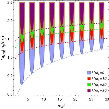
Figure 1: Parameter values and intervals of time for which $\omega_{k}^{2}<0$, indicated by the colored regions. The vertical axis is the ratio of the inflaton mass to the mass of the $\chi$ field. Roughly speaking, only for $\chi$ masses smaller than the $\phi$ mass can there be an instability. The different colors show the results for different values of $k$. For values of $k$ larger than $m_{\chi}$, it is the value of $k$ which determines if an instability is possible. It is infrared modes which can undergo the resonant excitation. The dashed lines indicate the lowest value of $m_{\phi}/m_{\chi}$ for which there can be a resonance.

From Fig. 1 we can see that for any sufficiently small values of $k$ and sufficiently small ratios for the masses, $m_{\chi}/m_{\phi}\ll 1$, the square of the frequency for the $\chi_{k}$ modes becomes negative. This happens twice every complete cycle of oscillation, in a time interval $-\pi/4<m_{\phi}\Delta t<\pi/4$. Since the maximal value of $k$ for which we expect resonance to happen, namely the $k_{max}$ given in (20), is a decreasing function of time, there willl be, for any value of $k$, a maximum time $t_{\rm max}$ for which $\omega_{k}^{2}$ can become negative. This maximal time (which depends on both $m_{\phi}$ and $m_{\chi}$) is indicated by the dashed lines in Fig. 1. For $t>t_{\rm max}$ there is no longer any exponential growth of $\chi_{k}$, and the modes simply oscillate after that time with the amplitude reached after the last instability region is crossed. This maximum time $t_{\rm max}$ is given by setting the cosine in Eq. (19) as one (i.e., at its maximum value) and solving the resulting equation for $\omega_{k}(t_{\rm max})=0$. This yields

$$m_{\phi}t_{\rm max}\,=\,$$

$$\left[3\frac{m_{\phi}^{2}}{m_{\chi}^{2}}+\frac{2k^{2}F(k,m_{\phi},m_{\chi})}{m_{\chi}^{2}\left(\frac{m_{\chi}}{m_{\phi}}\right)^{2/3}}-\frac{8k^{4}\left(\frac{m_{\chi}}{m_{\phi}}\right)^{2/3}}{3F(k,m_{\phi},m_{\chi})m_{\chi}^{4}}\right]^{1/2}\,,$$

(42)

where $F(k,m_{\phi},m_{\chi})$ in the above equation is given by

$$F(k,m_{\phi},m_{\chi})\,=\,3^{1/3}\left(-1+\sqrt{1+\frac{64k^{6}}{243m_{\phi}^{4}m_{\chi}^{2}}}\,\right)^{1/3}.$$ (43)

Note that for small values of $m_{\chi}$ (compared to $m_{\phi}$) the back-reaction of particle production on the inflaton condensate will shut off the resonance before $t_{max}$. This back-reaction time scale was discussed at the end of the previous section.

Neglecting the abovementioned back-reaction effect, the number of times an instability region is crossed for given values of $k,\,m_{\phi}$ and $m_{\chi}$ is given by

$$\Delta N\,=\,m_{\phi}t_{\rm max}/\pi\,.$$ (44)

For $k\ll m_{\chi}$, we have for instance that

$$\Delta N\,\sim\,m_{\phi}/(\pi m_{\chi})\,.$$ (45)

The smaller the ratio $m_{\chi}/m_{\phi}$, the larger will be the growth of the momentum modes for the $\chi$ field. The small oscillations of the metric induced by the oscillating inflaton can, therefore, as discussed in the previous section, be an efficient way of producing $\chi$-particles. Let us investigate this effect in more detail.

In Fig. 2 we consider the evolution of $\psi_{k}$ as a function of time $t$, in the case $k=0$ and $m_{\chi}\ll m_{\phi}$. As is evident, there is indeed resonant growth of the amplitude, as expected from the analytical analysis of the previous section. As expected based on our analytical approximations, the resonant growth is linear in time.

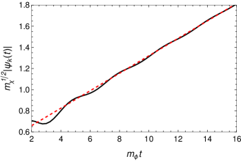
Figure 2: Time evolution of $\psi_{k}$ for $k=0$ and $m_{\chi}=10^{-6}m_{\phi}$ (solid black curve). The fit to a linear growth (red dashed curve) as a function of time is a good one, and it is found to be given by $|\psi_{k}(t)|\sim 0.0825(m_{\phi}t+6)/m_{\chi}^{1/2}$. We have used the usual vacuum initial conditions when solving for the mode equations, i.e., $\psi_{k}(t_{0})=e^{i\omega_{k}(t_{0})t_{0}}/\sqrt{2\omega_{k}(t_{0})}$ and $\dot{\psi}_{k}(t_{0})=ie^{i\omega_{k}(t_{0})t_{0}}\sqrt{\omega_{k}(t_{0})/2}$ and with $t_{0}$ set at $t_{R}=2/m_{\phi}$ [see Eq. (41)].

In Fig. 3, we show the numerical solution of the $\chi$-field momentum mode equation, Eq. (11), using Eq. (19), with $\psi_{k}(t)$ evaluated at the maximum time $t=t_{\rm max}$ at which the maximum amplitude for $\psi_{k}(t)$ is reached.

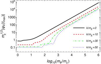
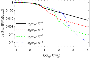
Figure 3: The modulus of $\psi_{k}(t)$ evaluated at the maximum time $t=t_{\rm max}$ and for different values of the ratio of masses $m_{\phi}/m_{\chi}$ and values of the momentum $k$. The evolution was started with vacuum initial conditions as in Fig. 2.

From Fig. 3, we see that $|\psi_{k}(t_{\rm max)}|$ can grow to larger values the smaller $m_{\chi}$ is compared to $m_{\phi}$. For $m_{\chi}\ll m_{\phi}$, when the results approach a linear behavior shown in Fig. 3, we have that $|\psi_{k}(t_{\rm max)}|$ can be well approximated by

$$|\psi_{k}(t_{\rm max)}|\simeq\frac{m_{\phi}}{4\pi m_{\chi}\left(k^{2}+m_{\chi}^{2}\right)^{1/4}}.$$ (46)

The results show that the condition $m_{\chi}\ll m_{\phi}$ is required in order to have an efficient resonance.

For illustrative purpose, we also show in Fig. 3 the amplitude of $|\psi_{k}(t_{\rm max)}|$, when normalized by its value at $k=0$, as a function of $k$. As expected, we see that for $k<m_{\chi}$ the growth rate is independent of $k$.

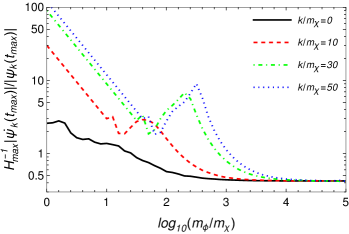
Figure 4: The growth rate for the modes computed at $t=t_{\rm max}$ normalized by the Hubble rate.

The rate of growth for the modes can be estimated by computing

$$\Gamma\,\equiv\,|\dot{\psi}_{k}/\psi_{k}|\,.$$ (47)

This rate is shown and compared to $H^{-1}$ in Fig. 4. Note that $\Gamma\gg H$, for values of $m_{\chi}$ which are not much smaller than $m_{\phi}$. But this is a region where the modes are not sufficiently excited. In the region where the modes experience pronounced growth (see Fig. 3), we have $\Gamma\simeq H/2$. Thus, as to be expected from the analytical analysis of the previous section, the resonance process is not fast on the Hubble time scale. Note, however, that the process is far more efficient than the usual graviton mediated decay channel for which the rate is given by the Eq. (50) shown in the following section.

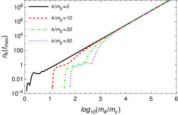
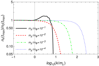
Figure 5: The comoving occupation number $n_{k}$ evaluated at $t=t_{\rm max}$. $n_{0}$ denotes the occupation number evaluated at vanishing momentum.

To illustrate the relative growth of the $\chi$-momentum modes, we can continue to work directly with the rescaled modes $\psi_{k}$, from which we have the adiabatic invariant for Eq. (11) with the interpretation of a comoving occupation number KLS2 ,

$$n_{k}\,=\,\frac{\omega_{k}}{2}\left(\frac{|\dot{\psi}_{k}|^{2}}{\omega_{k}^{2}}+|\psi_{k}|^{2}\right)-\frac{1}{2}.$$ (48)

In Fig. 5, we show the occupation number $n_{k}$ when computed at $t=t_{\rm max}$. As expected from the analytical analysis, the larger the ratio of $m_{\phi}/m_{\chi}$, the longer the period of resonance and the larger the value of $n_{k}$. Note that for $m_{\chi}\ll m_{\phi}$ the resonance is shut off for values of $k\gg m_{\chi}$ such $m_{\phi}\gg k\gg m_{\chi}$. The linear asymptotic behavior seen in Fig. 5 is well described by

$$n_{k}(t_{\rm max})\,\sim\,\sqrt{k^{2}+m_{\chi}^{2}}|\psi_{k}(t_{\rm max)}|^{2}/2\,,$$ (49)

with $|\psi_{k}(t_{\rm max)}|$ given by Eq. (46). As can also be seen in Fig. 5 and 5, for $k$ modes in the deep ultraviolet, the occupation number sharply drops as expected.

V Comparison with Perturbative Effects

In this section we wish to compare the resonant growth of $\chi$ particles with the perturbative growth which is obtained by the decay of the $\phi$ condensate mediated by gravitons. This decay width for this process was computed in Mambrini:2021zpp and takes the form

$$\Gamma_{\phi\phi\to\chi\chi}=\frac{\rho_{\phi}m_{\phi}}{1024\pi M_{\rm Pl}^{4}}\left(1+\frac{m_{\chi}^{2}}{2m_{\phi}^{2}}\right)^{2}\sqrt{1-\frac{m_{\chi}^{2}}{m_{\phi}^{2}}},$$ (50)

where $M_{\rm Pl}=1/\sqrt{8\pi G}$ is the reduced Planck mass, with $1/\sqrt{G}\equiv m_{\rm Pl}$ and $\rho_{\phi}$ is the energy density of the inflaton field. At the end of inflation (i.e., when the equation of state for the inflaton becomes larger than $-1/3$), we have that $\dot{\phi}_{\rm end}^{2}=V(\phi_{\rm end})$ and then

$$\rho_{\phi,{\rm end}}=\frac{3}{2}V(\phi_{\rm end})\,.$$ (51)

Assuming a quadratic potential for the inflaton field as in Eq. (2), we have

$$\phi_{\rm end}^{2}\,\simeq\,M_{\rm Pl}^{2}/(4\pi)\equiv 2M_{\rm Pl}^{2}$$ (52)

and hence

$$\rho_{\phi,{\rm end}}\,=\,3m_{\phi}^{2}M_{\rm Pl}^{2}$$ (53)

and $H_{\rm end}=m_{\phi}$. Recalling that for a quadratic inflaton potential normalized to get the right amplitude of curvature fluctuations we have

$$m_{\phi}\,\approx\,10^{-6}M_{\rm Pl}\,,$$ (54)

we find that

$$\Gamma_{\phi\phi\to\chi\chi}/H\,\sim\,10^{-9}\,.$$ (55)

From this discussion we conclude that the minimal preheating process discussed in this paper is many orders of magnitude more efficient that perturbative decay mediated by gravitons .

VI Conclusions

We have proposed a model-independent minimal preheating process which directly transfers the energy of the oscillating inflaton condensate to Standard Model particles, in particular the Higgs field. The effect is a consequence of a parametric resonance instability of tachyonic nature in the mode equation for scalar matter fields. This resonance is due to an oscillating contribution to the mass term of the modes which results from the oscillating pressure of the inflaton condensate. We have established a lower bound on the efficiency of the energy transfer. It leads to the decay of the condensate on a time scale given by (36), which is larger than the Hubble time at the end of inflation by a factor of the order of $10^{3}(m_{\rm Pl}/m_{\phi})^{3/2}$, where $m_{\phi}$ is the mass of the inflaton candidate. The effective temperature at the end of the dominance of the inflaton condensate is given by (39), which is smaller than the maximal temperature one could have expected by a factor of the order of $10^{-3/2}(Gm_{\phi}^{2})^{3/4}$.

Our analysis is based on an approximate analytical analysis in which we chose our approximations in order to under-estimate the strength of the effect. We confirmed the results using a numerical study of the solutions of the mode equation.

Previous studies of reheating focused on matter field excitations via matter couplings in the matter Lagrangian and are hence very model dependent. For large matter couplings, these non-gravitational channels can be more efficient than the one considered here, However, since we do not expect Standard Model particles to be directly coupled to the inflaton field, the previous mechanism leave open the question of energy transfer to Standard Model particles. An important aspect of our mechanism is that Standard Model particles are produced directly (and they are produced more efficiently than particles of a Beyond the Standard Model (BSM) if the masses of the BSM particles are much larger than those of Standard Model particles).

We have focused on the production of scalar field quanta. The same mechanism applies to gauge particle generation. A similar instability should also arise in the equation of motion for Fermions, but we expect that Pauli blocking will suppress the strength of Fermion particle production.

Our mechanism may have implications for the Dark Matter coincidence problem, namely the question of why the current energy densities of dark and visible matters are comparable. If Dark Matter is a very weakly interacting low mass (compared to the inflaton mass) scalar field, then during the phase of oscillations of the inflaton condensate the same energy density of dark matter and Higgs particles will be generated. How these densities evolve after the period of inflaton oscillations will be model dependent, and we will return to the study of this question in a future publication.