Quasar Luminosity Function at $z=7$

Abstract

We present the quasar luminosity function (LF) at $z=7$, measured with 35 spectroscopically confirmed quasars at $6.55<z<7.15$. The sample of 22 quasars from the Subaru High-$z$ Exploration of Low-Luminosity Quasars (SHELLQs) project, combined with 13 brighter quasars in the literature, covers an unprecedentedly wide range of rest-frame ultraviolet magnitudes over $-28<M_{1450}<-23$. We found that the binned LF flattens significantly toward the faint end populated by the SHELLQs quasars. A maximum likelihood fit to a double power-law model has a break magnitude $M^{*}_{1450}=-25.60^{+0.40}_{-0.30}$, a characteristic density $\Phi^{*}=1.35^{+0.47}_{-0.30}$ Gpc^-3 mag^-1, and a bright-end slope $\beta=-3.34^{+0.49}_{-0.57}$, when the faint-end slope is fixed to $\alpha=-1.2$ as observed at $z\leq 6$. The overall LF shape remains remarkably similar from $z=4$ to $7$, while the amplitude decreases substantially toward higher redshifts, with a clear indication of an accelerating decline at $z\geq 6$. The estimated ionizing photon density, $10^{48.2\pm 0.1}$ s^-1 Mpc^-3, is less than 1 % of the critical rate to keep the intergalactic medium ionized at $z=7$, and thus indicates that quasars are not a major contributor to cosmic reionization.

1 Introduction

We are witnessing rapid development in the quest for the most distant quasars, driven primarily by deep wide-field surveys at red-optical and near-infrared (IR) wavelengths. The first discoveries of high-$z$ ($z\geq 6$) quasars were achieved by the Sloan Digital Sky Survey (SDSS; e.g., Fan et al., 2006), which were soon followed by systematic identification of fainter co-eval quasars through surveys using the Canada–France–Hawaii Telescope (e.g., Willott et al., 2005). Subsequently, the sample size at the bright and faint ends has been expanded significantly by the Panoramic Survey Telescope And Rapid Response System 1 (Pan-STARRS1; e.g., Bañados et al., 2014) survey and the Hyper Suprime-Cam (HSC; Miyazaki et al., 2018) Subaru Strategic Program (SSP) survey (e.g., Matsuoka et al., 2016), among others. Near-IR surveys have pushed the frontier to yet higher redshifts, with the first $z>7$ quasar being found from the UKIRT Infrared Deep Sky Survey (Mortlock et al., 2011). The present redshift record is marked by a quasar at $z=7.642$ (Wang et al., 2021), identified from a combined dataset of several optical and near-IR surveys including the Wide-field Infrared Survey Explorer (WISE; Wright et al., 2010) survey. The advent of new world-leading projects in the coming few years, including the Vera C. Rubin Observatory Legacy Survey of Space and Time (LSST; Ivezić et al., 2019), Euclid, and the Roman Space Telescope (Spergel et al., 2015), is expected to accelerate the exploration further out to $z\sim 10$ (e.g., Euclid Collaboration et al., 2019).

One of the most fundamental quantities characterizing a population of celestial objects is the luminosity function (LF). In particular, the LF of high-$z$ quasars provides a key piece of information to decode the formation and evolution of supermassive black holes (SMBHs), as well as to measure the quasar contribution to cosmic reionization. The first attempts to measure the quasar LF at $z\sim 6$ were made with bright SDSS quasars at $M_{1450}<-25$ (Fan et al., 2004; Jiang et al., 2008, 2009). Willott et al. (2010) included fainter quasars to establish the LF over a broader luminosity range. This LF has been used as the standard in many subsequent studies, but the constraint on the faint end ($M_{1450}>-24$) was still weak, due to the small number of contributing objects. A robust measurement of the LF at $z=6$ down to well below the break luminosity ($-28<M_{1450}<-21$) was achieved by Matsuoka et al. (2018c), who exploited a large sample of faint quasars drawn from the HSC-SSP survey. Schindler et al. (2023) used Pan-STARRS quasars to further improve the bright-end constraint. At higher redshifts, Venemans et al. (2013) measured the cumulative number density using three luminous ($M_{1450}\sim-26$) quasars at $z\geq 6.6$. Wang et al. (2019) presented the number densities from 17 quasars at $z\sim 6.7$, measured in three magnitude bins from $M_{1450}\sim-27.5$ to $-25.5$. However, no other constraints have been reported to date, and thus the overall LF shape has not been determined beyond $z=6$.

Here we present a measurement of the quasar LF at $z=7$, based on an unprecedentedly large and complete sample of 35 quasars at $6.55<z<7.15$ covering a broad luminosity range. This is the 19th publication from the Subaru High-$z$ Exploration of Low-Luminosity Quasars (SHELLQs; Matsuoka et al., 2016) project, which performs spectroscopic identification and multi-wavelength follow-up observations of high-$z$ quasars drawn from the HSC-SSP imaging data (Aihara et al., 2018). Throughout the paper, we use point-spread-function (PSF) magnitudes ($m_{\rm AB}$) and associated errors ($\sigma_{\rm m})$ presented in the AB system (Oke & Gunn, 1983), corrected for Galactic extinction (Schlegel et al., 1998). The cosmological parameters of $H_{0}$ = 70 km s^-1 Mpc^-1, $\Omega_{\rm M}$ = 0.3, and $\Omega_{\rm\Lambda}$ = 0.7 are assumed.

2 Sample and methods

The present measurement combines two quasar samples, called the “bright sample” and the “faint sample” hereafter. They are summarized in Table 1 and are displayed in Figure 1. The bright sample is based on 17 quasars at $6.45<z<7.05$ presented by Wang et al. (2019). These quasars were identified from an effective area of 13,020 deg², using the imaging data from Pan-STARRS1, the DESI Legacy imaging Surveys (Dey et al., 2019), the UKIRT/VISTA Hemisphere Surveys, and the WISE survey. We selected 15 quasars at $z>6.55$ for the present purpose, and further removed two quasars with $y_{\rm AB}>20.8$ given that the spectroscopic follow-up at fainter magnitudes was incomplete (see Figure 8 of Wang et al., 2019).

The faint sample comes from SHELLQs, which has so far published the discovery of 162 low-luminosity quasars at $z>5.6$ (Matsuoka et al., 2016, 2018a, 2018b, 2019a, 2019b, 2022). The present analysis concerns $z$-band dropout sources with $y$-band detection, the signature of the Ly$\alpha$ break at $z\sim 7$. Spectroscopic identification has been completed for $z$-dropout candidates selected via a Bayesian probabilistic algorithm in the SSP public data release (DR) 3 fields (an effective area of 957 deg² with our quality cuts) and for those selected via color cuts in the SSP internal DR S20A fields (779 deg²; see Aihara et al., 2022). The details of the quasar selection criteria are described in Matsuoka et al. (2022). We use 22 SHELLQs quasars at $6.55<z<7.05$. There are a few more SHELLQs quasars in this redshift range, but they do not pass the selection algorithm with the quality flags and imaging properties taken from the latest DR. For example, the highest-redshift SHELLQs quasar at $z=7.07$ (Matsuoka et al., 2019b) and one of the faintest quasars with $z=6.72$ and $M_{1450}=-23.5$ (see Figure 1) happen to fall on regions affected by cosmic ray and a nearby bright star, respectively, and are thus excluded from the present measurement.

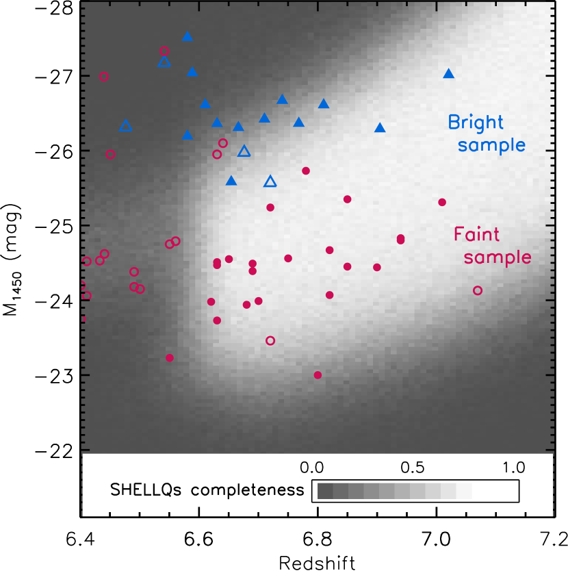
Figure 1: Quasars used for the LF determination by Wang et al. (2019, blue triangles) and those discovered by SHELLQs (red circles) over the $z$ – $M_{1450}$ plane. The quasars in the present LF sample are represented by the filled symbols, while all the others are represented by the open symbols. The background colors present completeness of the SHELLQs $z$-dropout selection from 0.0 (dark gray) to 1.0 (white).

Table 1: Quasar sample

Name	Redshift	$M_{1450}$
Bright sample (Wang et al. 2019)
$J$003836.10$-$152723.6	7.02	$-27.01$
$J$041128.63$-$090749.7	6.81	$-26.61$
$J$070626.38$+$292105.5	6.58	$-27.51$
$J$082931.98$+$411740.9	6.77	$-26.36$
$J$083737.83$+$492900.6	6.71	$-26.42$
$J$083946.88$+$390011.4	6.91	$-26.29$
$J$091054.54$-$041406.8	6.63	$-26.36$
$J$092347.12$+$040254.6	6.61	$-26.61$
$J$110421.58$+$213428.9	6.74	$-26.67$
$J$113508.92$+$501132.6	6.58	$-26.19$
$J$121627.58$+$451910.7	6.65	$-25.58$
$J$213233.18$+$121755.2	6.59	$-27.04$
$J$223255.16$+$293032.3	6.67	$-26.31$
Faint sample (SHELLQs)
$J$000142.54$+$000057.5	6.69	$-24.49$
$J$011257.84$+$011042.4	6.82	$-24.07$
$J$021316.94$-$062615.2	6.72	$-25.24$
$J$021430.90$+$023240.4	6.85	$-25.35$
$J$021847.04$+$000715.0	6.78	$-25.73$
$J$091041.14$+$005646.3	6.65	$-24.55$
$J$091906.33$+$051235.3	6.62	$-23.98$
$J$102314.45$-$004447.9	6.63	$-24.47$
$J$103537.74$+$032435.7	6.63	$-24.51$
$J$113034.65$+$045013.1	6.68	$-23.94$
$J$120505.09$-$000027.9	6.75	$-24.56$
$J$123137.77$+$005230.3	6.69	$-24.39$
$J$131050.13$-$005054.1	6.82	$-24.67$
$J$131746.92$+$001722.2	6.94	$-24.80$
$J$133833.25$-$001832.9	6.70	$-23.99$
$J$134905.63$+$015608.9	6.94	$-24.83$
$J$140344.28$+$423114.3	6.85	$-24.45$
$J$142903.08$-$010443.4	6.8	$-23.00$
$J$144045.91$+$001912.9	6.55	$-23.23$
$J$145005.39$-$014438.9	6.63	$-23.73$
$J$221027.24$+$030428.5	6.9	$-24.44$
$J$235646.33$+$001747.3	7.01	$-25.31$

The completeness, or selection function, of the bright sample has been kindly provided by F. Wang (private communication; see Figure 6 of Wang et al., 2019). For the faint sample, we derived the selection function using exactly the same method as described in Matsuoka et al. (2018c), which presents our LF measurement at $z=6$. We repeat only the essence in what follows. The detection probability of the HSC-SSP imaging for a given magnitude ($m_{\rm AB}$) has proven to be well approximated by the function

$$f_{\rm det}(m_{\rm AB})=\frac{1}{2}(\tanh[2.4(m_{\rm AB}^{5\sigma}-m_{\rm AB})]+1),$$ (1)

where $m_{\rm AB}^{5\sigma}$ is a 5$\sigma$ limiting magnitude measured for every 12′$\times$ 12′ patch of the survey footprint. SHELLQs selects point sources, whose completeness $f_{\rm ps}(m_{\rm AB})$ has been estimated with HSC-SSP sources observed by higher-resolution Hubble Space Telescope Advanced Camera for Surveys (Leauthaud et al., 2007); $f_{\rm ps}(m_{\rm AB})$ is always $>$80 % at the magnitudes we are concerned with ($y_{\rm AB}<24$ mag). We created mock high-$z$ quasars based on 319 SDSS spectra of luminous quasars at $z\simeq 3$, by shifting them to higher redshifts and applying Ly$\alpha$ absorption caused by the intergalactic medium (IGM; Songaila, 2004; Eilers et al., 2018). Each of the mock quasars was assigned random values of redshift, $M_{1450}$, and sky coordinates within the HSC-SSP survey footprint (and thus $m_{\rm AB}^{5\sigma}$), providing apparent magnitudes and errors.

We extracted a portion of the mock quasars, such that a quasar with magnitude $y_{\rm AB}$ has probability $f_{\rm det}(y_{\rm AB})\times f_{\rm ps}(y_{\rm AB})$ of being selected. The extracted quasars were then fed into the SHELLQs selection algorithm incorporating a Bayesian probabilistic approach and color cuts. The fraction of selected quasars among all the created mock quasars, as a function of $z$ and $M_{1450}$, provides the completeness. The reader is referred to Matsuoka et al. (2018c) for full details. The resultant completeness is presented in Figure 1. It indicates that our $z$-dropout selection is most sensitive to quasars at $z>6.6$. The low completeness at the bright end is due to our requirement of $i$-band non-detection for $z$-dropouts; luminous quasars could have detectable emission even in the Gunn & Peterson (1965) trough, and thus would not pass the selection. Indeed, the two SHELLQs quasars at $z\sim 6.65$ and $M_{1450}\sim-26.0$ (see Figure 1) are not in the present LF sample because of their $i$-band detection. The completeness remains high at $z>7.1$, although we found no quasars above $z=7.07$. While Ly$\alpha$ is well within the HSC $y$-band transmission up to $z\sim 7.5$, it is because (i) the $y$ band is progressively dominated by IGM absorption and (ii) Ly$\alpha$ shifts to the wavelength where the detector sensitivity is low. The imaging observations could thus detect only luminous quasars, which are too rare to be included in the $\sim$1000 deg² footprint of the SSP survey. We set the redshift interval of the present analysis to $6.55<z<7.15$, above which the completeness of the bright sample falls close to zero.

3 Results and Discussion

Figure 2 and Table 2 (top part) present the binned LF of the combined bright and faint sample, calculated with the 1/$V_{\rm a}$ method (Avni & Bahcall, 1980, see Equations 6 and 7 of Matsuoka et al. (2018c)) using the selection functions described above. For comparison, Figure 2 also shows the LFs of Lyman break galaxies at $z\sim 7$ measured by Harikane et al. (2022) and Varadaraj et al. (2023). Note that quasars or active galactic nuclei (AGNs) are not excluded from those LFs. There is some discrepancy between the two galaxy LFs, which Varadaraj et al. (2023) attribute to contamination of brown dwarfs to the bright end of the Harikane et al. (2022) sample. Overall, quasars are a dominant population of sources at $z\sim 7$ for $M_{1450}<-24$ ($y_{\rm AB}<23$), while galaxies quickly start to outnumber quasars at the fainter magnitudes.

We derived the parametric LF of the quasars assuming a double power-law model:

$$\Phi(M_{1450})=\frac{10^{k(z-7)}\Phi^{*}}{10^{0.4(\alpha+1)(M_{1450}-M_{1450}^{*})}+10^{0.4(\beta+1)(M_{1450}-M_{1450}^{*})}},$$ (2)

where $\alpha$ and $\beta$ are the faint- and bright-end slope, respectively, and $M^{*}_{1450}$ is the break magnitude. We determined the three parameters along with the normalization factor $\Phi^{*}$ with a maximum likelihood fit (Marshall et al., 1983, see Equation 9 of Matsuoka et al. (2018c)). We adopt the redshift-evolution slope of $k=-0.78$, which was measured between $z\sim 6$ and $z\sim 6.7$ by Wang et al. (2019). The best-fit parameters are reported in Table 2 (the first row of the bottom part), which yields the parametric LF presented in Figure 2 (dashed line). An alternative case with $k=-0.70$ (Jiang et al., 2016) was also tested but the results remain almost unchanged. It is remarkable that the parametric LF shows a positive faint-end slope ($\alpha>-1$; the number density declines toward the faint end), although a negative slope ($\alpha<-1$) is also allowed within the 2$\sigma$ confidence interval.

It is unlikely that our selection misses the faint-end quasars because of the extended emission from the host galaxies. Our criterion of point-source selection for $z$-dropouts is very conservative, $0.6<\mu$/$\mu_{\rm PSF}<3.0$, where $\mu$ and $\mu_{\rm PSF}$ represent the $y$-band image adaptive moment of a given source and that of the PSF model, respectively. That is, we allow the sources that are up to three times larger than the PSF size to remain in the candidates for spectroscopic confirmation. In reality, none of the SHELLQs quasars in the present sample has $\mu$/$\mu_{\rm PSF}>1.7$. All but a few of the $\sim$200 Lyman break galaxies at $z\sim 7$ with similar luminosities ($M_{1450}<-22$), drawn from the same HSC-SSP images (Harikane et al., 2022), also meet $\mu$/$\mu_{\rm PSF}<3.0$, even without the central point source (i.e., AGN).

A positive slope, if confirmed, might indicate that the obscured fraction increases and/or the mass-accretion efficiency decreases toward the low-mass end of the SMBH mass distribution at $z\geq 7$. Indeed, observations at lower redshifts ($z<4$) suggest that the obscured fraction increases significantly toward lower (intrinsic) luminosities (e.g., Merloni et al., 2014; Ueda et al., 2014; Toba et al., 2021). There is also an indication of a higher obscured fraction at higher redshifts up to $z\sim 6$ (e.g., Vito et al., 2018; Gilli et al., 2022). We have identified 23 candidate obscured quasars at $z\sim 6$ from SHELLQs (e.g., Matsuoka et al., 2022), based on the extremely luminous and narrow Ly$\alpha$ emission. Onoue et al. (2021) detected strong C IV $\lambda$1549 emission in one of them, pointing to the presence of hard ionizing radiation from AGN. A number of other observations (e.g., Fujimoto et al., 2022; Endsley et al., 2023) are revealing (candidates for) such a high-$z$ obscured population, and substantially more objects may be identified in the coming few years with the James Webb Space Telescope (JWST).

On the other hand, at lower redshifts ($z\leq 6$), the faint-end slope is close to flat but is always negative. For example, the measurements based on the HSC-SSP data suggest $\alpha=-1.30\pm 0.05$ at $z=4$ (Akiyama et al., 2018), $\alpha=-1.22^{+0.03}_{-0.10}$ at $z=5$ (Niida et al., 2020), and $\alpha=-1.23^{+0.44}_{-0.34}$ at $z=6$ (Matsuoka et al., 2018c). We thus performed another set of parametric fittings with a fixed slope of $\alpha=-1.2$. This case actually lies within the $\sim$2$\sigma$ confidence region when all four LF parameters are varied above, and indeed, the best-fit line with $\alpha=-1.2$ gives a reasonable agreement with the binned LF (see Figure 2). Therefore, we regard the case with $\alpha=-1.2$ (the third row in the bottom part of Table 2) as our standard fit to the quasar LF at $z=7$, and use the corresponding parameters in the following discussions. For reference, the table also lists the fitting results when two parameters, $\alpha$ and $M_{1450}$, are fixed to the values measured at $z=6$ (Matsuoka et al., 2018c).

Table 2: Quasar luminosity function at $z=7$

Binned luminosity function
$M_{1450}$	$\Delta M_{1450}$	$\Phi(M_{1450})$	$N_{\rm obj}$	$V_{\rm a}$
$-23.25$	0.5	2.5 $\pm$ 1.8	2	1.607
$-23.75$	0.5	3.0 $\pm$ 1.5	4	2.656
$-24.25$	0.5	3.5 $\pm$ 1.4	6	3.386
$-24.75$	0.5	3.2 $\pm$ 1.3	6	3.719
$-25.25$	0.5	1.58 $\pm$ 0.91	3	3.786
$-25.75$	0.5	0.75 $\pm$ 0.53	2	5.336
$-26.25$	0.5	0.63 $\pm$ 0.26	6	19.034
$-26.75$	0.5	0.18 $\pm$ 0.10	3	34.171
$-27.50$	1.0	0.082 $\pm$ 0.047	3	36.563
Parametric luminosity function
$\Phi^{*}$	$M_{1450}^{*}$	$\alpha$	$\beta$	$k$	comment
$4.75^{+1.14}_{-1.36}$	$-24.38^{+0.33}_{-0.47}$	$0.58^{+1.20}_{-0.93}$	$-2.78^{+0.28}_{-0.36}$	$-0.78$ (fixed)	free $\alpha$
$4.90^{+1.27}_{-1.43}$	$-24.40^{+0.35}_{-0.45}$	$0.52^{+1.24}_{-0.89}$	$-2.79^{+0.30}_{-0.35}$	$-0.70$ (fixed)	free $\alpha$, different $k$
$1.35^{+0.47}_{-0.30}$	$-25.60^{+0.40}_{-0.30}$	$-1.20$ (fixed)	$-3.34^{+0.49}_{-0.57}$	$-0.78$ (fixed)	standard
$2.07^{+0.17}_{-0.20}$	$-24.90$ (fixed)	$-1.23$ (fixed)	$-2.72^{+0.21}_{-0.22}$	$-0.78$ (fixed)	fixed $M_{1450}^{*}$

Note. — $M_{1450}$ and $\Delta M_{1450}$ denote the center and width of a magnitude bin, respectively, while $N_{\rm obj}$ represents the number of quasars contained in the bin. The number densities $\Phi(M_{1450})$ and $\Phi^{*}$ (normalization at $z=7$) are given in units of Gpc^-3 mag^-1. $V_{\rm a}$ (Gpc³) represents the cosmic volume available to discover quasars in the present sample.

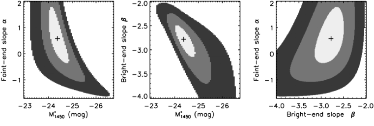
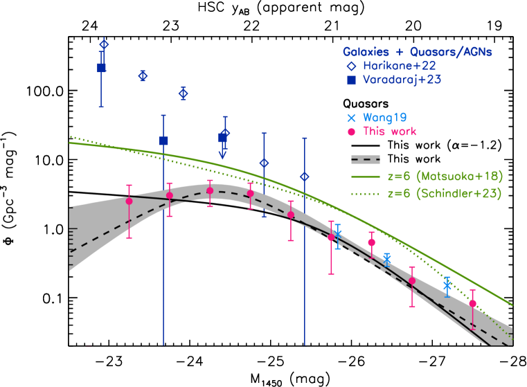
Figure 2: Top panels: confidence regions (light gray: 1$\sigma$, gray: 2$\sigma$, dark gray: 3$\sigma$) of the LF parameters. The best-fit values are marked by the crosses. Bottom panel: binned LF (red dots) and the standard parametric LF calculated at $z=6.8$ (solid line; the faint-end slope fixed to $\alpha=-1.2$) from this study. The dashed line and shaded area represent the best-fit and 1$\sigma$ confidence region, respectively, with $\alpha$ being a free parameter. For comparison, we also show the binned LF at $z=6.7$ (Wang et al., 2019, light-blue crosses) and the parametric LF measured at $z=6$ (Matsuoka et al. (2018c), green solid line; Schindler et al. (2023), green dotted line). The blue diamonds and squares represent the binned LF of Lyman break galaxies (AGNs are not excluded) at $z\sim 7$ taken from Harikane et al. (2022) and Varadaraj et al. (2023), respectively (slight horizontal offsets have been added to improve visibility). The upper axis gives approximate $y$-band magnitudes for a quasar at $z=6.8$.

Figure 3 (top panel) compares the quasar LFs at redshifts $z=4$, $5$, $6$, and $7$. The overall shape remains remarkably similar through this redshift range, while the amplitude decreases significantly toward higher redshift. Figure 3 (bottom panel) displays this decreasing trend more explicitly, with the data at $z<3.5$ supplemented from Kulkarni et al. (2019). The density peaks at lower redshifts for lower-luminosity quasars, an effect which is termed “down-sizing of AGNs” (Ueda et al., 2003; Barger et al., 2005). The cumulative number density declines rapidly toward higher redshifts following $\rho\propto 10^{-kz}$ with $k=-0.47$ (Fan et al., 2001) at $3<z<5$, and then it drops even faster at $z>5$. Jiang et al. (2016) reported $k=-0.72\pm 0.11$ at $5<z<6$, and Wang et al. (2019) found a steeper slope $k=-0.78\pm 0.18$ at $6<z<7$. While the above measurements were limited to the most luminous quasars ($M_{1450}<-26$ mag), Figure 3 suggests that the density of low-luminosity quasars ($M_{1450}<-23$) is also consistent with $k=-0.78$ at $5<z<7$. The similar epoch of turnover (i.e., to accelerating decline toward the highest redshifts) at different luminosities may indicate that the density evolution is governed by different physics from that drives the down-sizing at lower redshifts. Comparison of the present LF measurements with theoretical models (e.g., Li et al., 2022; Oogi et al., 2022) will be a subject of future papers.

Finally, we estimate the quasar contribution to cosmic reionization at $z=7$, using the LF estimated above. Section 5 of Matsuoka et al. (2018c) describes the details of this calculation. The ionizing photon density, $\dot{n}_{\rm ion}$, is calculated assuming that quasar spectra follow a broken power law (Lusso et al., 2015) and that a photon escape fraction is unity. By integrating our standard LF over $-30<M_{1450}<-18$, we get $\dot{n}_{\rm ion}=10^{48.2\pm 0.1}$ s^-1 Mpc^-3. This result is insensitive to the integrated magnitude range, since the LF is close to flat at the faint end and predicts a very small number of objects at the bright end. The value of the ionizing photon density that would balance the rate of recombination at $z=7$ is given by $\dot{n}_{\rm ion}=10^{50.2}C_{\rm HII}$ (s^-1 Mpc^-3), where $C_{\rm HII}$ represents an effective H II clumping factor (Madau et al., 1999; Bolton & Haehnelt, 2007). The observed $\dot{n}_{\rm ion}$ is thus less than 1 % of the critical density for any plausible value of $C_{\rm HII}\geq 1$, clearly suggesting that quasars cannot be a major contributor to the reionization of the universe at this redshift.

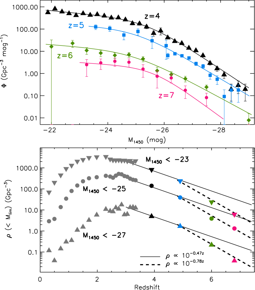
Figure 3: Evolution of the quasar LF. Top panel: binned and parametric LF of quasars at $z=4$ (black triangles and line; Akiyama et al., 2018), $z=5$ (blue squares and line; Niida et al., 2020), $z=6$ (green diamonds and line; Matsuoka et al., 2018c), and $z=7$ (red circles and line; this work). Bottom panel: integrated number density of quasars with $M_{1450}<-23$ (inverse triangles), $M_{1450}<-25$ (dots), and $M_{1450}<-27$ (triangles). The data at $z<3.5$ are taken from Kulkarni et al. (2019). Density evolution laws ($\rho\propto 10^{-kz}$) with $k=-0.47$ and $k=-0.78$ are represented by the solid and dashed lines, respectively, with arbitrary scaling.

The biggest original goal of the SHELLQs project was to establish the quasar LF at $6\leq z\leq 7$, which is now completed. The faint sample used here was drawn from the HSC-SSP data contained in the public DR 3, which have been acquired over 278 out of the 330 nights allocated to the SSP. The final DR, expected to happen in Fall 2023, will contain the data taken over the remaining 52 nights; we may use those data to further improve LF constraints, though it is not expected to increase the sample size significantly. In the meantime, the unprecedented sensitivity of JWST is starting to find signatures of low-mass AGNs in high-$z$ galaxies (e.g., Harikane et al., 2023; Larson et al., 2023; Onoue et al., 2023), and is also expected to shed new light on obscured side of the early AGN activity (e.g., Kocevski et al., 2023). With the advent of new cutting-edge facilities including the Rubin LSST, Euclid, and Roman, observations in the coming ten years will bring crucial constraints on the quasar/AGN LF out to very high redshifts, and thus will provide a key to discern models of the birth and growth of SMBHs throughout the epoch of reionization.

References

- Aihara et al. (2022) Aihara, H., AlSayyad, Y., Ando, M., et al. 2022, PASJ, 74, 247. doi:10.1093/pasj/psab122
- Aihara et al. (2018) Aihara, H., Arimoto, N., Armstrong, R., et al. 2018, PASJ, 70, S4
- Akiyama et al. (2018) Akiyama, M., He, W., Ikeda, H., et al. 2018, PASJ, 70, S34. doi:10.1093/pasj/psx091
- Avni & Bahcall (1980) Avni, Y. & Bahcall, J. N. 1980, ApJ, 235, 694. doi:10.1086/157673
- Bañados et al. (2014) Bañados, E., Venemans, B. P., Morganson, E., et al. 2014, AJ, 148, 14
- Barger et al. (2005) Barger, A. J., Cowie, L. L., Mushotzky, R. F., et al. 2005, AJ, 129, 578. doi:10.1086/426915
- Bolton & Haehnelt (2007) Bolton, J. S. & Haehnelt, M. G. 2007, MNRAS, 382, 325. doi:10.1111/j.1365-2966.2007.12372.x
- Dey et al. (2019) Dey, A., Schlegel, D. J., Lang, D., et al. 2019, AJ, 157, 168. doi:10.3847/1538-3881/ab089d
- Eilers et al. (2018) Eilers, A.-C., Davies, F. B., & Hennawi, J. F. 2018, ApJ, 864, 53. doi:10.3847/1538-4357/aad4fd
- Endsley et al. (2023) Endsley, R., Stark, D. P., Lyu, J., et al. 2023, MNRAS, 520, 4609. doi:10.1093/mnras/stad266
- Euclid Collaboration et al. (2019) Euclid Collaboration, Barnett, R., Warren, S. J., et al. 2019, A&A, 631, A85. doi:10.1051/0004-6361/201936427
- Fan et al. (2004) Fan, X., Hennawi, J. F., Richards, G. T., et al. 2004, AJ, 128, 515
- Fan et al. (2006) Fan, X., Strauss, M. A., Richards, G. T., et al. 2006, AJ, 131, 1203
- Fan et al. (2001) Fan, X., Strauss, M. A., Schneider, D. P., et al. 2001, AJ, 121, 54. doi:10.1086/318033
- Fujimoto et al. (2022) Fujimoto, S., Brammer, G. B., Watson, D., et al. 2022, Nature, 604, 261. doi:10.1038/s41586-022-04454-1
- Gilli et al. (2022) Gilli, R., Norman, C., Calura, F., et al. 2022, A&A, 666, A17. doi:10.1051/0004-6361/202243708
- Gunn & Peterson (1965) Gunn, J. E. & Peterson, B. A. 1965, ApJ, 142, 1633. doi:10.1086/148444
- Harikane et al. (2022) Harikane, Y., Ono, Y., Ouchi, M., et al. 2022, ApJS, 259, 20. doi:10.3847/1538-4365/ac3dfc
- Harikane et al. (2023) Harikane, Y., Zhang, Y., Nakajima, K., et al. 2023, arXiv:2303.11946. doi:10.48550/arXiv.2303.11946
- Ivezić et al. (2019) Ivezić, Ž., Kahn, S. M., Tyson, J. A., et al. 2019, ApJ, 873, 111. doi:10.3847/1538-4357/ab042c
- Jiang et al. (2008) Jiang, L., Fan, X., Annis, J., et al. 2008, AJ, 135, 1057
- Jiang et al. (2009) Jiang, L., Fan, X., Bian, F., et al. 2009, AJ, 138, 305
- Jiang et al. (2016) Jiang, L., McGreer, I. D., Fan, X., et al. 2016, ApJ, 833, 222. doi:10.3847/1538-4357/833/2/222
- Kocevski et al. (2023) Kocevski, D. D., Onoue, M., Inayoshi, K., et al. 2023, arXiv:2302.00012. doi:10.48550/arXiv.2302.00012
- Kulkarni et al. (2019) Kulkarni, G., Worseck, G., & Hennawi, J. F. 2019, MNRAS, 488, 1035. doi:10.1093/mnras/stz1493
- Larson et al. (2023) Larson, R. L., Finkelstein, S. L., Kocevski, D. D., et al. 2023, arXiv:2303.08918. doi:10.48550/arXiv.2303.08918
- Leauthaud et al. (2007) Leauthaud, A., Massey, R., Kneib, J.-P., et al. 2007, ApJS, 172, 219. doi:10.1086/516598
- Li et al. (2022) Li, W., Inayoshi, K., Onoue, M., et al. 2022, arXiv:2210.02308. doi:10.48550/arXiv.2210.02308
- Lusso et al. (2015) Lusso, E., Worseck, G., Hennawi, J. F., et al. 2015, MNRAS, 449, 4204. doi:10.1093/mnras/stv516
- Marshall et al. (1983) Marshall, H. L., Tananbaum, H., Avni, Y., et al. 1983, ApJ, 269, 35. doi:10.1086/161016
- Madau et al. (1999) Madau, P., Haardt, F., & Rees, M. J. 1999, ApJ, 514, 648. doi:10.1086/306975
- Matsuoka et al. (2022) Matsuoka, Y., Iwasawa, K., Onoue, M., et al. 2022, ApJS, 259, 18. doi:10.3847/1538-4365/ac3d31
- Matsuoka et al. (2019a) Matsuoka, Y., Iwasawa, K., Onoue, M., et al. 2019a, ApJ, 883, 183. doi:10.3847/1538-4357/ab3c60
- Matsuoka et al. (2018b) Matsuoka, Y., Iwasawa, K., Onoue, M., et al. 2018b, ApJS, 237, 5
- Matsuoka et al. (2016) Matsuoka, Y., Onoue, M., Kashikawa, N., et al. 2016, ApJ, 828, 26
- Matsuoka et al. (2018a) Matsuoka, Y., Onoue, M., Kashikawa, N., et al. 2018a, PASJ, 70, S35
- Matsuoka et al. (2019b) Matsuoka, Y., Onoue, M., Kashikawa, N., et al. 2019b, ApJ, 872, L2
- Matsuoka et al. (2018c) Matsuoka, Y., Strauss, M. A., Kashikawa, N., et al. 2018c, ApJ, 869, 150
- Merloni et al. (2014) Merloni, A., Bongiorno, A., Brusa, M., et al. 2014, MNRAS, 437, 3550. doi:10.1093/mnras/stt2149
- Miyazaki et al. (2018) Miyazaki, S., Komiyama, Y., Kawanomoto, S., et al. 2018, PASJ, 70, S1
- Mortlock et al. (2011) Mortlock, D. J., Warren, S. J., Venemans, B. P., et al. 2011, Nature, 474, 616
- Niida et al. (2020) Niida, M., Nagao, T., Ikeda, H., et al. 2020, ApJ, 904, 89. doi:10.3847/1538-4357/abbe11
- Oke & Gunn (1983) Oke, J. B., & Gunn, J. E. 1983, ApJ, 266, 713
- Onoue et al. (2023) Onoue, M., Inayoshi, K., Ding, X., et al. 2023, ApJ, 942, L17. doi:10.3847/2041-8213/aca9d3
- Onoue et al. (2021) Onoue, M., Matsuoka, Y., Kashikawa, N., et al. 2021, ApJ, 919, 61. doi:10.3847/1538-4357/ac0f07
- Oogi et al. (2022) Oogi, T., Ishiyama, T., Prada, F., et al. 2022, arXiv:2207.14689. doi:10.48550/arXiv.2207.14689
- Schindler et al. (2023) Schindler, J.-T., Bañados, E., Connor, T., et al. 2023, ApJ, 943, 67. doi:10.3847/1538-4357/aca7ca
- Schlegel et al. (1998) Schlegel, D. J., Finkbeiner, D. P., & Davis, M. 1998, ApJ, 500, 525
- Songaila (2004) Songaila, A. 2004, AJ, 127, 2598. doi:10.1086/383561
- Spergel et al. (2015) Spergel, D., Gehrels, N., Baltay, C., et al. 2015, arXiv:1503.03757. doi:10.48550/arXiv.1503.03757
- Toba et al. (2021) Toba, Y., Ueda, Y., Gandhi, P., et al. 2021, ApJ, 912, 91. doi:10.3847/1538-4357/abe94a
- Ueda et al. (2014) Ueda, Y., Akiyama, M., Hasinger, G., et al. 2014, ApJ, 786, 104. doi:10.1088/0004-637X/786/2/104
- Ueda et al. (2003) Ueda, Y., Akiyama, M., Ohta, K., et al. 2003, ApJ, 598, 886. doi:10.1086/378940
- Varadaraj et al. (2023) Varadaraj, R. G., Bowler, R. A. A., Jarvis, M. J., et al. 2023, arXiv:2304.02494. doi:10.48550/arXiv.2304.02494
- Venemans et al. (2013) Venemans, B. P., Findlay, J. R., Sutherland, W. J., et al. 2013, ApJ, 779, 24. doi:10.1088/0004-637X/779/1/24
- Vito et al. (2018) Vito, F., Brandt, W. N., Yang, G., et al. 2018, MNRAS, 473, 2378. doi:10.1093/mnras/stx2486
- Wang et al. (2021) Wang, F., Yang, J., Fan, X., et al. 2021, ApJ, 907, L1. doi:10.3847/2041-8213/abd8c6
- Wang et al. (2019) Wang, F., Yang, J., Fan, X., et al. 2019, ApJ, 884, 30. doi:10.3847/1538-4357/ab2be5
- Willott et al. (2005) Willott, C. J., Delfosse, X., Forveille, T., Delorme, P., & Gwyn, S. D. J. 2005, ApJ, 633, 630
- Willott et al. (2010) Willott, C. J., Delorme, P., Reylé, C., et al. 2010b, AJ, 139, 906
- Wright et al. (2010) Wright, E. L., Eisenhardt, P. R. M., Mainzer, A. K., et al. 2010, AJ, 140, 1868. doi:10.1088/0004-6256/140/6/1868