Simulating Gaussian Boson Sampling with Tensor Networks in the Heisenberg picture

Abstract

Although the Schrödinger and Heisenberg pictures are two equivalent formulations of quantum mechanics, simulations performed choosing one over the other can greatly impact the computational resources required to solve a problem. Here we demonstrate that in Gaussian boson sampling, a central problem in quantum computing, a good choice of representation can shift the boundary between feasible and infeasible numerical simulability. To achieve this, we introduce a novel method for computing the probability distribution of boson sampling based on the time evolution of tensor networks in the Heisenberg picture. This approach overcomes limitations of existing methods and enables, for example, simulations of realistic setups affected by non-uniform photon losses. Our results demonstrate the effectiveness of the method and its potential to advance quantum computing research.

I Introduction

Boson sampling is a challenging problem in the broad field of quantum computing that involves generating samples of integer tuples based on a specific probability distribution. For probability distributions that are hard to compute classically, previous research has shown that multimode quantum linear interferometers and projective measurements can solve this problem efficiently Aaronson and Arkhipov (2011). This solution provides evidence against the extended Church-Turing thesis, suggesting that passive linear optical machines are efficient, albeit non-universal, quantum computers that are available already today. Therefore, boson-sampling devices offer a practical alternative for efficiently solving computational problems that are not solvable by classical computers. Generating the necessary multimode highly indistinguishable Fock states poses experimental difficulties, as it typically requires postselection from two-mode squeezed (Gaussian) states obtained through low-power down conversion, with a huge impact on scalability. This challenge has prompted the exploration of alternative input states that are readily accessible yet maintain the computational complexity of the simulation problem. One notable accomplishment in this area is Gaussian boson sampling Rahimi-Keshari et al. (2015); Hamilton et al. (2017); Kruse et al. (2019), which does not require postselection and instead uses the entire field generated by the sources as a computational resource.

Figure 1: In the Schrödinger picture (left) we evolve the initial state of the bosonic modes $\ket{\psi}$ through a network of elementary two-mode gates implementing the target transformation $\mathcal{E}$, thus we can project the evolved state over the manifold of the output states $\ket{\mathbf{n}}$. Conversely, in the Heisenberg picture (right) we compute the expectation value of each projector $\mathbb{P}_{\mathbf{n}}$ after the evolution through to the map $\mathcal{E}^{*}$.

Although it is provably hard to simulate experimental boson sampling, even for devices with slight imperfections using classical methods, the extent to which current state-of the-art boson-samplers in the laboratory can achieve this regime remains an open question. The main classical algorithms for simulating boson sampling Quesada and Arrazola (2020); Quesada et al. (2022); Bulmer et al. (2022); Neville et al. (2017) rely on conditioned probability chain rules in order to construct good output sequences element by element, at the price of computing a restricted number of analytical probabilities or, even dealing with restricted family of experimental imperfections Oh et al. (2023), on an approximation of the distribution. Phase space representation of linear optics has been successfully employed for verification of boson sampling experiments Drummond et al. (2022). Tensor networks Orús (2019); Montangero (2018); Schollwöck (2011) offer an approximate representation of the quantum state of radiation in linear quantum optics experiments allowing for controlled errors Lubasch et al. (2018). The complexity of the representation using tensor networks in Boson sampling is directly linked to the correlations that develop among photons during their physical evolution, which is a significant factor that makes the problem computationally hard. The original formulation of both Fock and Gaussian boson sampling fully characterises the ideal case. Recent advances came from considering how the boson sampling probability distribution changes under partial photon distinguishability Renema (2020); Shi and Byrnes (2022). The effect of losses on the overall complexity of the sampling problem has been explored in Qi et al. (2020). One additional benefit of the tensor network formalism is the possibility to easily and flexibly include the most important experimental imperfections in simulations, in particular, photon losses, and probe their effects on the microscopical dynamics of the bosonic wavefunction. It is worth noting that common to all formulations of boson sampling is the detection scheme or, in other words, the relevant observable. These are Fock space projectors or, in the case of threshold detectors, incoherent mixtures of them. Boson sampling experiments yield probability estimates for these observables but not of the entire quantum state of the device while the standard tensor network simulations yield the entire state, i.e. more information than is actually needed to model the experiment. Furthermore, it is well known that multi-mode correlations in a boson sampler grow rapidly, similar to those following a sudden quench, which imply in the worst case an exponential growth in the bond-dimension. This suggests that further efficiency gains may be possible in classical tensor network simulations by transitioning them from the evolution of the wave-function to one where one evolves the desired observables instead. Indeed, it has been demonstrated for an Ising model under a sudden quench that simulation of the wave-function dynamics in the Schrödinger picture scales exponentially in the quench time Schuch et al. (2008) while the evolution of a desired observable in the Heisenberg picture scales linearly in time Hartmann et al. (2009); Clark et al. (2010); Muth et al. (2011). This motivates the approach in this work to simulate the dynamics of a boson sampler through tensor networks in the Heisenberg picture by evolving each projector instead of the input state. We derive the exact scaling of the maximally required bond dimension of bosonic tensor networks evolving through a series of local two-body interactions and use this to demonstrate that in the simulation of boson sampling devices the transition to the Heisenberg picture can yield an exponential advantage in terms of the required simulation resources as compared to the Schrödinger picture simulations. We also note that our technique does not only allow us to account for a wide variety of imperfections and decoherence and dissipation mechanisms, including the important effects due to photon loss on the target probability distribution but that it is also not limited to the Gaussian boson sampling protocol since in the Heisenberg picture we can easily move to other input states, even correlated ones, with limited additional costs that can be kept under control.

II Gaussian Boson Sampling

This section presents basic definitions and notation that will be used in the remainder of this work.

Definition 1 (Gaussian boson sampling Kruse et al. (2019)).

Let $\hat{\mathcal{U}}$ be an $M\times M$ unitary matrix, $\ket{\psi}=\bigotimes_{j=0}^{M}\hat{S}_{r_{j}}\ket{0}_{j}$ a tensor product of $M$ harmonic oscillator squeezed vacuum states and $\ket{\mathbf{n}}=\ket{n_{1},n_{2},\ldots,n_{M}}$ a multi-mode Fock state with the k-th mode containing $n_{k}$ bosons. Then, given the probability

$$p_{\mathbf{n}}=|\langle\mathbf{n}\,|\,\hat{\mathcal{U}}\,|\,\psi\rangle|^{2}\equiv P_{\rm GBS}(\mathbf{n})=\frac{1}{\mathbf{n}!\sqrt{|\sigma_{Q}|}}{\rm Haf}(A_{S})\,,$$ (1)

where $\sigma_{Q}=\sigma+\mathbb{I}_{2M}/2$, with $\sigma_{ij}=\langle\{\hat{\zeta}_{i},\hat{\zeta}_{j}^{\dagger}\}\rangle_{\psi}/2-\langle\hat{\zeta}_{i}\rangle_{\psi}\langle\hat{\zeta}_{j}\rangle_{\psi}$ defined as the covariance matrix of $\ket{\psi}$ with $\{\hat{\zeta}\}=\{\hat{a}_{1},\ldots,\hat{a}_{M},\hat{a}^{\dagger}_{1},\ldots,\hat{a}^{\dagger}_{M}\}$, and

$$A=\Biggl{(}\begin{matrix}0&\mathbb{I}_{M}\,\\ \mathbb{I}_{M}\,&0\end{matrix}\Biggr{)}(\mathbb{I}_{M}-\sigma_{Q}^{-1})\,,$$ (2)

generating a sample of strings $\{\mathbf{n}\}$ distributed according to (1) is the Gaussian boson sampling problem.

The Hafnian of a $M\times M$ square matrix $A$ is defined as

$${\rm Haf}(A)=\sum_{\mu\in{\rm PMP}}\prod_{j=1}^{N}{A}_{\mu(2j-1),\mu(2j)}\,,$$ (3)

with $N<M$ and ${\rm PMP}$ is the set of all the perfect matching permutations of the string $s=\{1,2,\ldots,2M\}$, i.e. all the permutations with the structure $\{a(1),b(1),a(2),b(2)\ldots a(M),b(M)\}$ with $a,b\in s$ such that $a(i)<b(i)\,\forall i$ and $a(i)<a(j)\,\forall i<j$ Callan (2009). Computing this Hafnian requires $\mathcal{O}(M^{2}2^{M/2})$ arithmetic operations, rendering the related sampling problem intractable on classical computers. As for Fock boson sampling Aaronson and Arkhipov (2011), the problem in Definition 1 can be mapped into a measurement task: a set of $M$ single-mode squeezed photonic states evolves through a passive linear interferometer implementing the unitary $\hat{\mathcal{U}}$, then photon-counting is performed on the output states, yielding a string $\mathbf{n}$ distributed according to eq. (1) Kruse et al. (2019). For squeezed vacuum input, the output state, $\hat{\mathcal{U}}\ket{\psi}$, of an ideal $M$-mode Gaussian boson sampling experiment in the Fock basis is a coherent superposition of all the $M$-mode Fock states with an even number of photons. Nevertheless the target probability distribution eq. 1 is encoded in ${\rm diag}\{\rho_{\rm out}\}={\,\rm diag}\{\,\hat{\mathcal{U}}\,|\psi\rangle\langle\psi|\,\hat{\mathcal{U}}^{\dagger}\}$, i.e. only part of the information encoded in the output state is relevant. Up to now the main approach for simulating boson sampling with tensor networks consisted in evolving the multimode squeezed state $\ket{\psi}$ under the action of the unitary $\hat{\mathcal{U}}$ and finally computing the probability of a particular outcome $\mathbf{n}$ through the projection of the evolved state over $\ket{\mathbf{n}}$ García-Patrón et al. (2019); Liu et al. (2023). Here, in contrast, we solve the problem in the Heisenberg picture, i.e. we evolve our observables that are described by the projectors $\mathbb{P}_{\mathbf{n}}\coloneqq|\mathbf{n}\rangle\langle\mathbf{n}|$, instead of the input state (see Fig. 1):

$$p_{\mathbf{n}}={\rm Tr}\{\mathcal{E}(|\psi\rangle\langle\psi|)\mathbb{P}_{\mathbf{n}}\}\rightarrow{\rm Tr}\{|\psi\rangle\langle\psi|~{}\mathcal{E}^{*}(\mathbb{P}_{\mathbf{n}})\}\,,$$ (4)

where the map $\mathcal{E}$ acting on the input state implements the evolution induced by the passive linear optical transformation ($\hat{\mathcal{U}}$ and any other channel, including losses). Even if the two pictures are physically equivalent, in many cases of interest Hartmann et al. (2009) it has been proved that the dynamical production of entanglement in the evolution of many body systems makes the time propagation of the MPS representation of the entire state very inefficient compared to that of some classes of observables. As it will be clear in section V, analogous conclusions hold for boson sampling.

III Tensor network representation of a multiphoton interferometer

We represent the $M$-mode GBS setup as a tensor network as shown in Nüßeler et al. (2021). The input state is represented by a tensor product of $M$ squeezed vacuum states

$$\ket{\Psi}=\bigotimes_{i=0}^{M}\hat{S}(r_{i})\ket{0}\,,$$ (5)

where $r_{i}$ is the squeezing parameter of the radiation in the $i$-th input mode and the squeezing operator reads

$$\hat{S}(r_{i})={\rm exp}\{r_{i}(\hat{a}_{i}^{2}-\hat{a}_{i}^{{\dagger}2})\}\,$$ (6)

where $\{\hat{a}_{i},\hat{a}_{i}^{\dagger}\}$ are the ladder operators of the quantum harmonic oscillator representing the $i$th mode. In the following we will assume for definiteness $r_{i}=r\,\forall i$. The local dimension of each harmonic oscillator is truncated at $n_{c}$. The choice of this cut-off is crucial for the accuracy and the performance of the simulation and depends critically on the loss rate of the architecture (see next section for a detailed discussion). The interferometer is implemented through the action of a series of local gates acting on pairs of modes. Each local gate $\hat{G}$ is a beamsplitter followed by a local phase shift operation

$$\hat{U}_{\theta,\varphi}={\rm exp}\{i\theta(\,\hat{a}_{i}\,\hat{a}_{i+1}^{\dagger}e^{-i\varphi}+{\rm H.c.})\}\,,$$ (7)

$$\hat{P}_{\phi}={\rm exp}\{i\phi\,\hat{a}_{i}^{\dagger}\,\hat{a}_{i}\}\,,$$ (8)

$$\hat{G}_{\theta,\varphi,\phi}=\hat{U}_{\theta\varphi}\cdot\hat{P}_{\phi}\,.$$ (9)

After the action of each $2$-mode gate the corresponding tensor network is compressed with a maximum allowed bond dimension $D_{\rm max}$ that is chosen in order to ensure convergence. If we assume the same local dimension $n_{c}$ for each oscillator, the computational cost of the action of each single gate is $o(n_{c}^{4}D_{\rm max}^{2}+n_{c}^{2}D_{\rm max}^{3})$. With the aim of representing a realistic setup, we consider the interferometer as a sequence of $d$ layers made of $(M-1)/2$ two-mode gates alternatively arranged (see Fig. 1). In this case, as typically $n_{c}\ll D_{max}$, the complexity of the tensor network algorithm reads

$$c\sim o(Md\,n_{c}^{2}D_{\rm max}^{3})\,.$$ (10)

The Clements protocol allows to represent any unitary acting on $M$-modes as a circuit with depth $d=M$ through a polynomial-time algorithm Clements et al. (2016). Thus in the lossless case we map the problem into a tensor network with $M(M-1)/2$ gates and the complexity of our algorithm reads

$$c\sim o(M^{2}n_{c}^{2}D_{\rm max}^{3})\,.$$ (11)

Note that this estimate is general and holds both for the Schrödinger and the Heisenberg picture. The choice of the picture will make the difference in the behaviour of $D$ with the depth of the circuit and the required choice of $D_{\rm max}$.

IV Losses and local dimension cutoff

The standard way to describe a lossy optical mode $a$ is to couple it with an external mode $\eta$ acting as environment and then operate a partial trace over the latter: if the initial state of the environment is the vacuum state $\ket{0}_{\eta}$ we yield a dynamical map $\mathcal{D}$ defined by a set of Kraus operators

$$\hat{K}_{\mu}=\,_{\eta}\langle\mu|\hat{\mathcal{W}}_{a\eta}|0\rangle_{\eta}\,,$$ (12)

where $\hat{\mathcal{W}}_{a\eta}=\hat{U}_{\alpha,0}$ (see (13)) with $\gamma={\rm sin}^{2}(\alpha)\ll 1$ i.e. a high-transmittivity beam splitter: the reflected part of the radiation is lost. Despite the simplicity of this solution, adopting it in the Heisenberg picture requires some care. The evolution of a couple of projectors $\langle\hat{O}\rangle\in\mathcal{H}^{\otimes 2}$ through a lossy gate reads

$$\langle\hat{O}^{\prime}\rangle =\rm{Tr}\Big{\{}\sum_{\mu}\hat{K}_{\mu}\,\hat{\mathcal{U}}\,\rho\,\hat{\mathcal{U}}^{\dagger}\hat{K}_{\mu}^{\dagger}\hat{O}\Big{\}}$$

$$=\rm{Tr}\Big{\{}\sum_{\mu}\,\rho~{}\hat{\mathcal{U}}^{\dagger}\hat{K}_{\mu}^{\dagger}\hat{O}\,\hat{K}_{\mu}\hat{\mathcal{U}}\Big{\}}\,,$$ (13)

thus in the vectorized representation the evolved projector is

$$\ket{\hat{O}^{\prime}}=\hat{\mathcal{U}}^{\dagger}\otimes\hat{\mathcal{U}}^{T}\sum_{\mu}\hat{K}_{\mu}^{\dagger}\otimes\hat{K}_{\mu}^{T}\ket{\hat{O}}\,.$$ (14)

Note that the Kraus map acting on $\hat{O}$ in the Heisenberg picture is $\mathcal{D}^{*}$. The resulting non-trace-preserving evolution will create excitations, which typically increases the required choice for the cutoff dimension of the mode’s Hilbert spaces. We can workaround this problem with a preliminary analysis of the probability distribution Eq. (1) and with a simple statistical argument: in the Heisenberg picture each lossy gate is turned into an independent stochastic source of photons with rate $\gamma$. The probability of generating $x$ photons from $Q$ sources at rate $\gamma$ is well approximated by the binomial

$$\pi_{\gamma}(x)=\binom{Q}{x}\gamma^{x}(1-\gamma)^{Q-x}\,,$$ (15)

while the probability of generating $\nu$ couples of photons from M single-mode sources sharing the same squeezing amplitude $r$ reads Kruse et al. (2019)

$$P_{M}^{r}(2\nu)=\binom{\nu+M/2-1}{\nu}{\rm sech}^{M}(r){\rm tanh}^{2\nu}(r)\,.$$ (16)

In the ideal case we can reconstruct the distribution Eq. (1) from Eq. (16) since they are related by

$$P^{r}_{M}(\tilde{n})=\sum_{\mathbf{n}\in{\omega_{\tilde{n}}}}p_{\mathbf{n}}\,,$$ (17)

where $\omega_{\tilde{n}}$ is the set of the outcomes $\mathbf{n}$ with fixed number of excitation $\tilde{n}$. The same operation in a lossy setup yields

$$P^{r}_{M\gamma}(\tilde{n})=\sum_{\mathbf{n}\in{\omega_{\tilde{n}}}}p_{\mathbf{n}}^{\gamma}\,,$$ (18)

where $p^{\gamma}_{\mathbf{n}}$ is the unknown lossy GBS probability distribution. In general for a fixed number of photons $\tilde{n}$, we expect to find $P^{r}_{M\gamma}(\tilde{n})\neq P^{r}_{M}(\tilde{n})$ since the losses create an unbalance between the probability to generate a $\tilde{n}$-photon component in input and the probability to observe an outcome configuration with the same number of photons. In particular losses will enhance the probability to observe outcomes with $\tilde{n}$ photons at the expenses of the probabilities of outcomes with $n>\tilde{n}$ photons. Considering only the positive contribution, we easily find the upper bound

$$P^{r}_{M\gamma}(\tilde{n})-P^{r}_{M}(\tilde{n})\leq\Delta_{\gamma}(\tilde{n})\coloneqq\sum_{x>0}\pi_{\gamma}(x)P^{r}_{M}(\tilde{n}+x)\,.$$ (19)

For $\tilde{n}$ sufficiently large we expect this difference to vanish since $P^{r}_{M}(n)$ decays exponentially with $n$. On the other hand this implies that, in the presence of losses, the contribution of the states from subspaces with $n>\tilde{n}$ is exponentially suppressed. In the Heisenberg picture this means that we can neglect the components of $\hat{O}^{\prime}$ featuring more than $\tilde{n}$ photons with a maximum error of the order of $\Delta_{\gamma}(\tilde{n})$. Thus we define the cutoff value ${n}_{c}$ for the local dimension of the oscillators as the value $n$ for which

$$\Delta_{\gamma}(n={n}_{c})<\epsilon\,,$$ (20)

where $\epsilon\ll 1$ is an arbitrary threshold. In the experimental regime of interest $\gamma$ is sufficiently small (significant losses can degrade the interference effects and make the problem more tractable for classical computers) and $d<\gamma^{-1}$, thus the main contribution to (19) comes from $P_{\gamma}(1)$, i.e. only the subspace with $\tilde{n}+1$ excitations have to be considered.

V Bond dimension scaling

In this section we derive the scaling of the bond dimension that permits exact representation of the Heisenberg operator for the lossless Fock boson sampling (FBS) dynamics. In the lossless case we can replace each projector $\mathbb{P}_{\mathbf{n}}$ with the corresponding quantum state $\ket{\mathbf{n}}=\prod_{k}{\hat{a}^{{\dagger}\,n_{k}}_{k}}\ket{{\rm vac}}$. As a result, the problem can be transformed into investigating the time evolution of the creation operators. For the sake of argument we assume the total number of photons $n<M$ (this condition is typically required to ensure the computational hardness of boson sampling Kruse et al. (2019)). The propagation of a single photon in a linear optical network featuring $M$ modes and at least $M$ layers generates a delocalized single-photon state that reads

$$\mathcal{U}(\hat{a}^{\dagger}_{k})\ket{\rm vac}=\sum_{i=0}^{M}u_{ik}\hat{a}^{\dagger}_{i}\ket{\rm vac}\,,$$ (21)

where $\hat{a}_{k}^{\dagger}=\bigotimes_{i=0}^{k-1}\mathbb{1}_{i}\otimes\hat{a}_{k}^{\dagger}\otimes\bigotimes_{i=k+1}^{M}\mathbb{1}_{i}$. With respect to any bipartition ($A,B$) of the support, an evolved single-photon state can be decomposed as

$$\mathcal{U}(\hat{a}_{k}^{\dagger})=\sum_{j\in A}u_{kj}\hat{a}_{j}^{\dagger}\otimes\mathbb{1}_{B}+\mathbb{1}_{A}\otimes\sum_{j\in B}u_{kj}\hat{a}_{j}^{\dagger}\,,$$ (22)

that’s equivalent to a W state. Thus the operator $\mathcal{U}(\hat{a}^{{\dagger}}_{k})=\hat{\mathcal{U}}\,\hat{a}^{{\dagger}}_{k}\,\hat{\mathcal{U}}^{\dagger}$ can be represented as an ${\rm MPO}$ with maximum bond dimension $2$. More in general, for $n$ photons in the same mode we have the multiphoton operator

$$\mathcal{U}(\hat{a}_{k}^{{\dagger}\,n})=\sum_{k=0}^{n}\binom{n}{k}\bigg{(}\sum_{j\in A}u_{kj}\hat{a}_{j}^{\dagger}\bigg{)}^{n-k}\!\!\!\!\!\!\otimes\bigg{(}\sum_{j\in B}u_{kj}\hat{a}_{j}^{\dagger}\bigg{)}^{k}\,$$ (23)

that generates a state with at most $n+1$ independent components and is represented by an MPO with maximum bond dimension $D=n+1$.

In the case with $n$ input photons over a generic set of modes $s_{m}$ with size $m\leq n$ we have

$$\mathcal{U}(\prod_{k\in s_{m}}\hat{a}^{{\dagger}\,n_{k}}_{k})\ket{\rm vac}=\prod_{k\in s_{n}}\mathcal{U}(\hat{a}^{{\dagger}\,n_{k}}_{k})\ket{\rm vac}\,,$$ (24)

where, in the last step, we have the product of $n$ MPOs each with maximum bond dimension $n_{k}+1$. Thus for the maximum bond dimension of an MPS representing a $n$-photon state we find the bound

$$D_{\rm max}^{\rm FBS}=\prod_{k\in s_{m}}(n_{k}+1)\leq 2^{n}\,.$$ (25)

where the equality holds when $n=m$, i.e. the upper bound is reached when all the input photons are injected through distinct ports. This is somehow reminiscent of the fact that calculating the permanents of matrices containing repeated rows or columns may be comparatively simpler than calculating the permanents of non-repetitive matrices Aaronson and Hance (2012). Investigating this connection is beyond the scope of this paper, and it would be worthwhile to explore it in future research. When $n\gtrsim M$ we observe a slight reduction of the bond dimension while remaining exponential in relation to the number of photons (see appendix A).

In the case of Gaussian input states the state (5) is injected through each mode and the number of photons is not fixed. Therefore in this case we can span the whole space state until the bond dimension is saturated (see appendix A for details):

$$D_{\rm max}^{\rm GBS}\sim n^{M/2}\,.$$ (26)

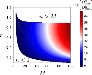
Figure 2: Maximum bond dimension scaling: Schrödinger vs Heisenberg in the ideal case. We compare $D_{\rm max}^{S}$ and $D_{\rm max}^{H}$ (Eqs. (26) and (25)) as functions of the number of modes $M$ and the squeezing parameter $r$ in the regime of validity of the bond dimension scaling Eq. (25) ($1<n={\rm mode}[P_{M}^{r}]<M$).

The adoption of the Heisenberg picture reduces the task of computing a single bin $p_{\mathbf{n}}$ of the GBS probability distribution to a FBS taking as input $\mathbb{P}_{\mathbf{n}}$, followed by the projection over the squeezed input state (which can be computed in polynomial time), therefore in the Heisenberg picture $D_{\rm max}^{H}\!=\!D_{\rm max}^{\rm FBS}$ (while in the Schrödinger picture $D_{\rm max}^{S}=D_{\rm max}^{\rm GBS}$). Remarkably, the maximum bond dimension in the Heisenberg picture does not depend directly on the number of modes $M$, but only on the number of photons $n$ in each probe output configuration $\mathbf{n}$. On the other hand, according to (16), the larger $M$, the more photons in the output configurations we must include in order to describe a significant part of the output distribution. A comparison between the scaling of the bond dimension in the Schrödinger and in the Heisenberg picture is reported in Fig. 2. For each couple of parameters $(r,M)$, the reference photon number is $n={\rm mode}[P_{M}^{r}]=2(M/2-1){\rm sinh}^{2}(r)$. We restrict to the regime $1<{\rm mode}[P_{M}^{r}]<M$ for which (25) strictly holds. For $n\geq M$ photon bunching reduces the maximum bond dimension resulting in a better scaling (see Appendix A).

We can immediately see that, even for moderate squeezing, in the Schrödinger picture the bond dimension grows dramatically as $M$ increases. Conversely, the Heisenberg picture is advantageous in the near classically hard regime. Plugging (25) into (10), for the lossless evolution of a $n$-photon state we get,

$$c_{H}\sim o(Md\,n_{c}^{2}\,2^{3n})\,,$$ (27)

that in the lossy case is turned into

$$c_{H}\sim o(Md\,n_{c}^{2}\,2^{3n_{c}})\,,$$ (28)

since the evolution (14) in the worst case generates up to $n_{c}$ additional excitations.

VI Conclusions

In this paper we have demonstrated that the Heisenberg picture may provide significant advantage in simulating the time evolution of bosonic many body systems. In the case of ideal Gaussian boson sampling, the evolution of squeezed vacuum states through passive linear optical networks yields a strongly correlated state whose numerical representation through MPS is in general very demanding in computational resources. The scaling in Eq. (28) is notably worse than that of the best algorithms for computing Hafnians and permanents. This is not surprising since each evolved projector carries the information of a whole family of correlated Hafnians depending on the squeezed state we choose as input state and not only a single one. Our tensor network protocol allows to compute $p(\mathbf{n})$ in the presence of several types of experimental imperfections, in particular beyond the limit of uniform losses, while an analytical closed form of the probability taking these effects into account is still unknown. In addition, the Heisenberg picture evolution allows to draw the probability distribution of several types of boson sampling protocols through changes in the state $|\psi\rangle$ (e.g. for simulating Fock boson sampling) that are free of additional cost or switch to classical superpositions of projectors as observables (boson sampling with threshold detectors Quesada et al. (2018)). Even if computing each bin of the target probability requires the simulation of the action of the whole interferometer on each observable of interest, the scaling of the bond dimension (Fig. 2) makes this procedure rapidly advantageous with respect to the Schrödinger picture evolution in the nearly classically hard regime. Furthermore, the independent nature of individual tasks and the modularity of tensor networks enable different levels of parallelization, which can be efficiently exploited by utilizing GPU cluster computing. This is especially beneficial when dealing with a significant number of output configurations.

VII Acknowledgements

This work was supported by the BMBF project PhoQuant (grant no. 13N16110) and the state of Baden-Württemberg through bwHPC and the German Research Foundation (DFG) through grant no INST 40/575-1 FUGG (JUSTUS 2 cluster). D.C. would like to thank T. Ilias and G. Di Meglio for fruitful discussions.

Appendix A Bond dimension scaling with $n\gtrsim M$

The MPO (24) can be expressed as follows when considering a symmetric bipartition

$$\mathcal{U}(\prod_{k\in s_{m}}\hat{a}^{{\dagger}\,n_{k}}_{k})=\sum_{k=0}^{N}\sum_{i}\lambda_{i}^{(k)}\hat{L}^{i}_{k}\otimes\hat{R}^{i}_{N-k}\,,$$ (29)

where the index $i$ runs over all the independent components with fixed number of photons $k$ and $N-k$ on the left and the right partition respectively, $\hat{L}_{k}$ ($\hat{R}_{N-k}$) is a product of $k$ ($N-k$) creation operators $\hat{a}^{\dagger}_{j}$ and $M/2-k$ ($M/2-(N-k)$) identities $\mathbb{1}_{j}$ in all possible arrangements with $j\in[0,M/2-1]$($[M/2,M]$). Note that when the number of photons in one partition is fixed, the number of photons in the other partition is automatically determined since the evolution preserves $N$. The maximum bond dimension $D_{\rm max}$ is given by the number of coefficients $\lambda_{i}^{(k)}$ with multiplicity, i.e. the sum over all the possible $k$ of the minimum number of independent components over the two partitions. Given $k$ input photons in one partition, each component corresponds to a subset of cardinality $k$ of a set of cardinality $M/2+k-1$ Flajolet and Sedgewick (2009). Thus a reasonable upward estimate is

$$D_{\rm max}=\sum_{k=0}^{N}{\rm min}\left\{\binom{m_{L}-1+k}{k}\,,\,\binom{m_{R}-1+(N-k)}{(N-k)}\right\}\,,$$ (30)

where $m_{L}$ and $m_{R}$ is the number of modes of the left and the right partition respectively and we consider the possibility of having an odd number of modes (i.e.  $m_{L}$ and $m_{R}$ can differ by one). Considering, for the sake of clarity, an even number of modes, so that $m_{L}=m_{R}=M/2$, we have

$$D_{\rm max}=\begin{cases}2\sum_{k=0}^{N/2-1}\binom{\frac{M}{2}-1+k}{k}+\binom{\frac{M+N}{2}-1}{\frac{N}{2}}&\text{, $N$ even;}\\ 2\sum_{k=0}^{(N-1)/2}\binom{\frac{M}{2}-1+k}{k}&\text{, $N$ odd.}\end{cases}$$ (31)

Given that

$$\binom{\frac{M}{2}-1+k}{k}=\frac{M/2}{M/2+k}\binom{\frac{M}{2}+k}{k}\,,$$ (32)

$$\binom{\frac{M}{2}+k}{k}<\binom{N}{k}~{}~{}{\rm for}~{}N\geq M\,,$$ (33)

and considering that

$$2^{N}=\sum_{k=0}^{N}\binom{N}{k}=2\sum_{k=0}^{N/2-1}\binom{N}{k}+\binom{N}{N/2}\,,$$ (34)

we find $D_{\rm max}<2^{N}$.

Finally, it should be noted that each component of the photonic squeezed state described in equation (5) possesses a distinct number of photons. Thus in this case the correspondence between the numbers of photons in the left and right partition does not hold. Consequently, assuming the local dimension cutoff $n_{c}$, in the Schrödinger picture each individual independent component corresponds to an $M/2$-tuple over the set $\{0,1,\ldots,n_{c}\}$ and we obtain the upper bound (26).

References

- Aaronson and Arkhipov (2011) Scott Aaronson and Alex Arkhipov, “The computational complexity of linear optics,” in Proceedings of the forty-third annual ACM symposium on Theory of computing (2011) pp. 333–342.
- Rahimi-Keshari et al. (2015) Saleh Rahimi-Keshari, Austin P. Lund, and Timothy C. Ralph, “What can quantum optics say about computational complexity theory?” Physical Review Letters 114, 060501 (2015).
- Hamilton et al. (2017) Craig S Hamilton, Regina Kruse, Linda Sansoni, Sonja Barkhofen, Christine Silberhorn, and Igor Jex, “Gaussian boson sampling,” Physical review letters 119, 170501 (2017).
- Kruse et al. (2019) Regina Kruse, Craig S. Hamilton, Linda Sansoni, Sonja Barkhofen, Christine Silberhorn, and Igor Jex, “Detailed study of gaussian boson sampling,” Phys. Rev. A 100, 032326 (2019).
- Quesada and Arrazola (2020) Nicolás Quesada and Juan Miguel Arrazola, “Exact simulation of gaussian boson sampling in polynomial space and exponential time,” Physical Review Research 2, 023005 (2020).
- Quesada et al. (2022) Nicolás Quesada, Rachel S. Chadwick, Bryn A. Bell, Juan Miguel Arrazola, Trevor Vincent, Haoyu Qi, and Raúl GarcíaPatrón, “Quadratic speed-up for simulating gaussian boson sampling,” PRX Quantum 3, 010306 (2022).
- Bulmer et al. (2022) Jacob F. F. Bulmer, Bryn A. Bell, Rachel S. Chadwick, Alex E. Jones, Diana Moise, Alessandro Rigazzi, Jan Thorbecke, Utz-Uwe Haus, Thomas Van Vaerenbergh, Raj B. Patel, Ian A. Walmsley, and Anthony Laing, “The boundary for quantum advantage in gaussian boson sampling,” Science Advances 8, eabl9236 (2022).
- Neville et al. (2017) Alex Neville, Chris Sparrow, Raphaël Clifford, Eric Johnston, Patrick M. Birchall, Ashley Montanaro, and Anthony Laing, “Classical boson sampling algorithms with superior performance to near-term experiments,” Nature Physics 13, 1153–1157 (2017).
- Oh et al. (2023) Changhun Oh, Liang Jiang, and Bill Fefferman, “On classical simulation algorithms for noisy boson sampling,” (2023), arXiv:2301.11532 [quant-ph] .
- Drummond et al. (2022) Peter D. Drummond, Bogdan Opanchuk, A. Dellios, and M. D. Reid, “Simulating complex networks in phase space: Gaussian boson sampling,” Phys. Rev. A 105, 012427 (2022).
- Orús (2019) Román Orús, “Tensor networks for complex quantum systems,” Nature Reviews Physics 1, 538–550 (2019).
- Montangero (2018) Simone Montangero, Introduction to tensor network methods (Springer Cham, 2018).
- Schollwöck (2011) Ulrich Schollwöck, “The density-matrix renormalization group in the age of matrix product states,” Annals of Physics 326, 96–192 (2011).
- Lubasch et al. (2018) Michael Lubasch, Antonio A. Valido, Jelmer J. Renema, W. Steven Kolthammer, Dieter Jaksch, M. S. Kim, Ian Walmsley, and Raúl García-Patrón, “Tensor network states in time-bin quantum optics,” Phys. Rev. A 97, 062304 (2018).
- Renema (2020) Jelmer J. Renema, “Simulability of partially distinguishable superposition and gaussian boson sampling,” Phys. Rev. A 101, 063840 (2020).
- Shi and Byrnes (2022) Junheng Shi and Tim Byrnes, “Effect of partial distinguishability on quantum supremacy in gaussian boson sampling,” npj Quantum Information 8, 54 (2022).
- Qi et al. (2020) Haoyu Qi, Daniel J. Brod, Nicolás Quesada, and Raúl García-Patrón, “Regimes of classical simulability for noisy gaussian boson sampling,” Phys. Rev. Lett. 124, 100502 (2020).
- Schuch et al. (2008) N Schuch, M M Wolf, K G H Vollbrecht, and J I Cirac, “On entropy growth and the hardness of simulating time evolution,” New Journal of Physics 10, 033032 (2008).
- Hartmann et al. (2009) Michael J. Hartmann, Javier Prior, Stephen R. Clark, and Martin B. Plenio, “Density matrix renormalization group in the heisenberg picture,” Phys. Rev. Lett. 102, 057202 (2009).
- Clark et al. (2010) Stephen R Clark, Javier Prior, Michael J Hartmann, Dieter Jaksch, and Martin B Plenio, “Exact matrix product solutions in the heisenberg picture of an open quantum spin chain,” New Journal of Physics 12, 025005 (2010).
- Muth et al. (2011) Dominik Muth, Razmik G Unanyan, and Michael Fleischhauer, “Dynamical simulation of integrable and nonintegrable models in the heisenberg picture,” Physical Review Letters 106, 077202 (2011).
- Callan (2009) David Callan, “A combinatorial survey of identities for the double factorial,” (2009), 10.48550/arxiv.0906.1317.
- García-Patrón et al. (2019) Raúl García-Patrón, Jelmer J. Renema, and Valery Shchesnovich, “Simulating boson sampling in lossy architectures,” Quantum 3, 169 (2019).
- Liu et al. (2023) Minzhao Liu, Changhun Oh, Junyu Liu, Liang Jiang, and Yuri Alexeev, “Complexity of gaussian boson sampling with tensor networks,” (2023), 10.48550/arxiv.2301.12814.
- Nüßeler et al. (2021) Alexander Nüßeler, Ish Dhand, Susana F. Huelga, and Martin B. Plenio, “Efficient construction of matrix-product representations of many-body gaussian states,” Phys. Rev. A 104, 012415 (2021).
- Clements et al. (2016) William R. Clements, Peter C. Humphreys, Benjamin J. Metcalf, W. Steven Kolthammer, and Ian A. Walmsley, “Optimal design for universal multiport interferometers,” Optica 3, 1460–1465 (2016).
- Aaronson and Hance (2012) Scott Aaronson and Travis Hance, “Generalizing and derandomizing gurvits’s approximation algorithm for the permanent,” (2012), arXiv:1212.0025 [quant-ph] .
- Quesada et al. (2018) Nicolás Quesada, Juan Miguel Arrazola, and Nathan Killoran, “Gaussian boson sampling using threshold detectors,” Physical Review A 98, 062322 (2018).
- Flajolet and Sedgewick (2009) Philippe Flajolet and Robert Sedgewick, Analytic Combinatorics, 1st ed. (Cambridge University Press, USA, 2009).