A generalization of photon sphere based on escape/capture cone

Abstract

In asymptotically flat spacetimes, bearing the null geodesics reaching the future null infinity in mind, we propose new concepts, the “dark horizons” as generalizations of the photon sphere. They are defined in terms of the structure of escape/capture cones of photons with respect to a unit timelike vector field. More specifically, considering a two-sphere that represents a set of emission directions of photons, the dark horizons are located at positions where a hemisphere is marginally included in the capture and escape cones, respectively. We show that both of them are absent in the Minkowski spacetime, while they exist in spacetimes with black hole(s) under a certain condition. We derive the general properties of the dark horizons in spherically symmetric spacetimes and explicitly calculate the locations of the dark horizons in the Vaidya spacetime and the Kerr spacetime.

E0,E31,A13

1 Introduction

Recently, Event Horizon Telescope (EHT) Collaboration succeeded in obtaining the image of the regions around black holes in M87 Akiyama:2019cqa and in Sagittarius A* EventHorizonTelescope:2022xnr . Future observations of the black hole shadow are expected to test the general relativistic magnetohydrodynamics (GRMHD) models EventHorizonTelescope:2019pgp , to constrain theories of gravity Wang:2018prk ; Moffat:2019uxp ; Khodadi:2020gns , and so forth. In static and spherically symmetric spacetimes, the edge of the shadow is given by the photon sphere Virbhadra:1999nm ; Claudel:2000 . Following the definition of Ref. Claudel:2000 , the photon sphere is provided as a $SO(3)\times{\mathbb{R}}$-invariant photon surface in a static and spherically symmetric spacetime. Here, the photon surface is defined as a nowhere-spacelike hypersurface $S$ such that, any null geodesic tangent to $S$ at any point on $S$ is included in $S$. Interestingly, the outermost photon sphere has been shown to satisfy the areal inequality Yang:2019zcn (see also Lu:2019zxb )

$$\frac{9}{4}A_{H}\leq A_{\rm ph,out}\leq A_{\rm sh,out}\leq 36\pi M^{2},$$ (1)

where $A_{H}$ is the area of the event horizon, $A_{\rm ph,out}$ is the area of the outermost photon sphere, $A_{\rm sh,out}$ is the area of the shadow observed at infinity, and $M$ is the Arnowitt-Deser-Misner (ADM) mass.

There have been several attempts to generalize the photon sphere in which new concepts are defined with local geometrical quantities Shiromizu:2017ego ; Yoshino:2017gqv ; Cao:2019vlu ; Yoshino:2019dty . From the observational point of view, however, the global analysis for the orbits of the photons is crucial. For example, in Refs. Siino:2019vxh ; Siino:2021kep , the approach based on the existence of an infinite number of conjugate points along a null geodesic congruence is adopted.

In this paper, we introduce new generalizations of the photon sphere, which we name the outer dark horizon (ODH) and the inner dark horizon (IDH), to capture the observability of photon sources from future null infinity. In order to consider the photon sources, we introduce a unit timelike vector $T^{\mu}$. In the frame associated with $T^{\mu}$, the escape/capture cones can be defined, and these two dark horizons are determined by the structure of those cones. Therefore, these new concepts refer to the condition for null geodesics from the sources to reach future null infinity In this point, our definition is different from the wandering geodesic defined in Refs. Siino:2019vxh ; Siino:2021kep in which the light sources are supposed to be located at past null infinity.

The rest of this paper is organized as follows. In Sec. 2, we provide a brief review of the asymptotic behavior of null geodesics near future null infinity as a preparation. In Sec. 3, we introduce the ODH and IDH as generalizations of the photon sphere in general asymptotically flat spacetimes. In Sec. 4, we focus on a static and spherically symmetric case as a specific example. In Sec. 5, we see their properties in the Vaidya spacetime as a simple example of dynamical spacetimes. In Sec. 6, we investigate the ODH and IDH in the Kerr spacetime as an example of spacetimes with angular momenta. The last section gives a summary and discussions. In Apps. A and B, we provide detailed explanations of a lemma in Sec. 4 and inequalities in Sec. 6, respectively. We use the units in which the speed of light and the Newtonian constant of gravitation are unity, $c=1$ and $G=1$. We assume the metric to be $C^{2-}$ functions (i.e., class $C^{1,1}$). The metric sign convention is $(-,+,+,+)$ in this paper.

2 Review of Null Asymptotics in the Bondi coordinate

In this section, as a preparation for the proof of Lem. 3.13 and Lem. 3.17, we review the asymptotic behavior of the metric and null geodesics near future null infinity in four-dimensional asymptotically flat spacetimes. The detailed analyses are presented in Refs. Amo:2021gcn ; Amo:2021rxr ; Amo:2022tcg ; Amo:2023qws .

We begin with reviewing the Bondi coordinate based on Refs. Bondi ; Sachs , which describes the asymptotic behavior of the metric near future null infinity (for the generalization to higher dimensions, see also Refs. Tanabe:2011es ; Hollands:2003ie ; Hollands:2003xp ; Ishibashi:2007kb ). The non-zero components of the metric near future null infinity in the Bondi coordinates can be expanded in the power of $1/r$ as

$$g_{uu} = -1+mr^{-1}+{{\cal O}\left(r^{-2}\right)},$$ (2)

$$g_{ur} = -1+{{\cal O}\left(r^{-2}\right)},$$ (3)

$$g_{IJ} = h_{IJ}r^{2}~{}=~{}\omega_{IJ}r^{2}+h^{(1)}_{IJ}r+{{\cal O}\left(r^{0}\right)},$$ (4)

$$\quad g_{uI} = {{\cal O}\left(r^{0}\right)}.$$ (5)

Here, $u$ denotes the retarded time, $r$ is the areal radius, $x^{I}$ stands for the angular coordinates, and $\omega_{IJ}$ is the metric for the unit two-sphere. The non-zero components of the inverse metric behave as

$$g^{ur} = -1+{{\cal O}\left(r^{-2}\right)},$$ (6)

$$g^{rr} = 1-mr^{-1}+{{\cal O}\left(r^{-2}\right)},$$ (7)

$$g^{rI} = {{\cal O}\left(r^{-2}\right)},$$ (8)

$$g^{IJ} = \omega^{IJ}r^{-2}-h^{(1)IJ}r^{-3}+{{\cal O}\left(r^{-4}\right)},$$ (9)

where $\omega^{IJ}$ is the inverse of $\omega_{IJ}$, and $h^{(1)IJ}$ is defined as $h^{(1)IJ}:=\omega^{IK}\omega^{JL}h^{(1)}_{KL}$. Future null infinity is supposed to be in the limit of $r\to\infty$ while $u$ is kept finite. Let us impose the gauge condition

$$\sqrt{\det h_{IJ}}=\omega_{2},$$ (10)

where $\omega_{2}$ is the volume element of the two-dimensional unit sphere. Here, $h_{IJ}-\omega_{IJ}$ corresponds to gravitational waves. In general relativity, the integration of $m(u,x^{I})$ over the angular coordinates gives us the Bondi mass,

$$M(u):=\frac{1}{8\pi}\int_{S^{2}}md\Omega.$$ (11)

Next, let us review the asymptotic behavior of null geodesics near future null infinity based on Refs. Amo:2021gcn ; Amo:2021rxr ; Amo:2022tcg ; Amo:2023qws . By combining the $r$-component of the geodesic equation and the condition for the geodesic to be null, we have

$$r^{\prime\prime} = \Omega_{IJ}r\left(x^{I}\right)^{\prime}\left(x^{J}\right)^{\prime}+{{\cal O}\left(r^{0}\right)}\left|\left(x^{I}\right)^{\prime}\right|^{2}+{{\cal O}\left(r^{-2}\right)}r^{\prime 2},$$ (12)

where $\Omega_{IJ}$ is defined as

$$\Omega_{IJ}:=\omega_{IJ}-\frac{1}{2}\frac{\partial h^{(1)}_{IJ}}{\partial u}+\frac{1}{2}\frac{\partial m}{\partial u}\omega_{IJ}.$$ (13)

Here, the prime denotes the derivative with respect to the affine parameter. We also define $\Omega\left(u,{x^{I}};dx^{J}/du\right)$ and $\Omega_{i}$ as

$$\Omega\left(u,{x^{I}};\frac{dx^{J}}{du}\right) := \left(\omega_{IJ}\frac{dx^{I}}{du}\frac{dx^{J}}{du}\right)^{-1}\Omega_{KL}\left(u,{x^{M}}\right)\frac{dx^{K}}{du}\frac{dx^{L}}{du},$$ (14)

$$\Omega_{i} := \inf_{u,{x^{I}},dx^{J}/du}\Omega\left(u,{x^{I}};\frac{dx^{J}}{du}\right).$$ (15)

Note that the magnitude of $dx^{J}/du$ does not affect the value of $\Omega\left(u,{x^{I}};dx^{J}/du\right)$. In Refs. Amo:2021gcn ; Amo:2022tcg ; Amo:2023qws , the careful analysis of the global behavior of null geodesics with Eq. (12) gives us a sufficient condition to reach future null infinity. In particular, the result for $\Omega_{i}>0$, which we use later, is given by the following statement:

Proposition 2.1.

Consider a four-dimensional asymptotically flat spacetime with $\Omega_{i}>0$ in which the metric near future null infinity is written as Eqs. (2)–(5) with the Bondi coordinates by $C^{2-}$ functions. We define $\beta_{\rm crit}$ as

$$\beta_{\rm crit}:=\frac{-3+\sqrt{9-6\Omega_{i}}}{3}.$$ (16)

Take a point $p$ with a sufficiently large radial coordinate value $r=r_{0}$. Any null geodesic emanating from $p$ reaches future null infinity if

$$0<\left(\left.\frac{dr}{du}\right|_{p}-\beta_{\rm crit}\right)^{-1} = o\left(r_{0}^{~{}}\right)$$ (17)

holds.

Here, Eq. (17) roughly means $dr/du|_{p}\gtrsim\beta_{\rm crit}$. In the case with $\partial m/\partial u$ and $\partial h^{(1)}_{IJ}/\partial u$ being small enough, which corresponds to the situation that matter radiations and gravitational waves are both weak enough near future null infinity, the value of $\beta_{\rm crit}$ is appropriately given by $\beta_{\rm crit}\approx-(1-1/\sqrt{3})\approx-0.423$. By this proposition, we see that photons emitted with $dr/du\geq 0$ and ones with $dr/du={{\cal O}\left(r_{0}^{~{}-1}\right)}$ reach future null infinity under the assumptions in the proposition. For higher dimensions, see Refs. Amo:2021gcn ; Amo:2022tcg .

3 Outer Dark Horizon and Inner Dark Horizon

In this section, we introduce two new concepts, “outer dark horizon (ODH)” and “inner dark horizon (IDH),” as generalizations of the photon sphere in general asymptotically flat spacetimes. The definitions of the ODH and IDH refer to future null infinity as the event horizon does.

This section is organized as follows. In subsection 3.1, we present the definitions of the ODH and IDH, and discuss their properties. In subsection 3.2, the relation of the ODH and IDH to the escape and capture cone is discussed. In subsections 3.3 and 3.4, we examine the properties of the ODH and IDH, respectively.

3.1 Basics of Outer Dark Horizon and Inner Dark Horizon

In this subsection, we introduce the outer dark horizon (ODH) and the inner dark horizon (IDH) as generalizations of the photon sphere by examining whether photons emitted from photon sources reach future null infinity or not. The ODH and IDH are defined as the boundary of “outer dark domain (ODD)” and “inner dark domain (IDD)”, respectively, which are also defined below.

Let ${\mathcal{M}}$ be a four-dimensional asymptotically flat and connected spacetime, and $T^{\mu}$ be a unit timelike vector field with $T_{\mu}T^{\mu}=-1$.

Definition 3.1 (outer dark domain (ODD) associated with $T^{\mu}$)

Suppose a set $S$ consists of all $p\in\mathcal{M}$ satisfying the following condition: for all spacelike vectors $n^{\mu}$ orthogonal to $T^{\mu}$ at $p$, there exists a null geodesic emanating from $p$, whose tangent vector $k^{\mu}$ is orthogonal to $n^{\mu}$ at $p$, such that it will not reach future null infinity. Then, we call $S$ the outer dark domain (ODD) associated with $T^{\mu}$.

Definition 3.2 (outer dark horizon (ODH) associated with $T^{\mu}$)

Let a region $S$ be the ODD associated with $T^{\mu}$ in ${\mathcal{M}}$. Then, the boundary $\partial S$ is called the outer dark horizon (ODH) associated with $T^{\mu}$.

Definition 3.3 (inner dark domain (IDD) associated with $T^{\mu}$)

Suppose a set $S$ consists of all $p\in\mathcal{M}$ satisfying the following condition: there exists a spacelike vector $n^{\mu}$ orthogonal to $T^{\mu}$ at $p$, such that all null geodesics emanating from $p$ whose tangent vector $k^{\mu}$ is orthogonal to $n^{\mu}$ at $p$ will not reach future null infinity $\mathscr{I}^{+}$. Then, we call $S$ the inner dark domain (IDD) associated with $T^{\mu}$.

Definition 3.4 (inner dark horizon (IDH) associated with $T^{\mu}$)

Let a region $S$ be the IDD associated with $T^{\mu}$ in ${\mathcal{M}}$. Then, the boundary $\partial S$ is called the inner dark horizon (IDH) associated with $T^{\mu}$.

The outer dark domain and the inner dark domain are sometimes simply called the dark domains as a set. Similarly, the outer dark horizon and the inner dark horizon are simply called the dark horizons. The ODD and IDD are complementary concepts to each other in the sense that the roles of “there exists” and “for all” are switched in the definitions. We required the vector $n^{\mu}$ to be orthogonal to $T^{\mu}$ in the definitions of 3.1 and 3.3 in order to consider the escape condition of photons in the frame associated with $T^{\mu}$. As a result, the locations of dark domains and dark horizons depend on the choice of $T^{\mu}$, which is arbitrarily chosen. The reason why we normalized $T^{\mu}$ is that only the direction of $T^{\mu}$, but not its norm, is important in the above definitions. Note that the norm of $n^{\mu}$ also has no effect in the definitions. One natural choice is to take $T^{\mu}$ as tangent vectors of the light source orbits. In this case, the escape condition of the emitted photon depends on the motion of the sources due to the effect of the relativistic beaming. In spacetimes with symmetries, it is also natural to construct $T^{\mu}$ using the time coordinate, which will be adopted in Secs. 4, 5 and 6. Here, it is also possible to consider situations where $T^{\mu}$ is defined only in a subregion of the spacetime and define the dark domain and dark horizon in this subregion, but we mainly focus on situations where $T^{\mu}$ is defined globally in the whole spacetime.

In addition, we can consider a particular class of the outer/inner dark domain/horizon. Suppose a time coordinate $t$ is present, and a spacelike hypersurface $\Sigma_{t}$ is given by $t=\mathrm{constant}$. From the time coordinate $t$, we can naturally introduce a timelike unit vector field by

$$T^{\mu}\ =\ \frac{-\nabla^{\mu}t}{\sqrt{-\nabla^{\nu}t\nabla_{\nu}t}}.$$ (18)

Adopting this vector field as $T^{\mu}$ in the definitions of the ODD and IDD, we can introduce outer/inner dark domain/horizon associated with the time slice $\Sigma_{t}$ as follows:

Definition 3.5 (outer/inner dark domain/horizon associated with $\Sigma_{t}$)

Suppose a time coordinate $t$ is present, and the spacelike hypersurface $t=$constant is denoted as $\Sigma_{t}$. The ODD/IDD and the ODH/IDH associated with the timelike vector field $T^{\mu}=-\nabla^{\mu}t/\sqrt{-\nabla^{\nu}t\nabla_{\nu}t}$ are called the ODD/IDD and the ODH/IDH associated with time slice $\Sigma_{t}$.

For the outer/inner dark domain/horizon associated with $\Sigma_{t}$, the vector $n^{\mu}$ in the definitions of 3.1 and 3.3 is tangent to $\Sigma_{t}$.

In Sec. 4, we will show that the ODH and IDH are generalizations of the “visible photon sphere,” which is defined in Def. 4.2 as an important class of the photon sphere. We will also see that they are both absent in the Minkowski spacetime and both exist in a spacetime with black hole(s) under certain conditions. These facts imply that the existence of the ODH/IDH is expected to be an indicator for the existence of a strong gravity region. The words “outer” and “inner” refer to the fact that the IDD is generally included by the ODD, which will be confirmed in Cor. 3.9.

The ODH and IDH refer to the condition for null geodesics to reach future null infinity. Here, null geodesics reaching future null infinity are of importance in observations of black holes because the observers, which can be regarded as staying at future null infinity, receive signals of photons that propagate along null geodesics. Since the geodesic equations are second-order differential equations, the initial position and its first derivative provide us with the unique solution . Therefore, at any point in the spacetimes, the emission angle of a photon (in the frame of the photon source) determines whether it reaches future null infinity or not.

3.2 Relation to escape and capture cones

The escape cone is a useful concept to describe the condition for photons to reach future null infinity. In order to explain this concept, we introduce the tetrad basis, $T^{\mu}$ and $(e_{i})^{\mu}$ with $i=1,2$, and $3$, and the projection tensor $\gamma_{\mu\nu}=g_{\mu\nu}+T_{\mu}T_{\nu}$ onto the three-dimensional spacelike tangent subspace spanned by $(e_{i})^{\mu}$. Then, the emission direction in the frame of the photon source is expressed by the vector

$$E^{\mu}\,=\,\frac{k_{\perp}^{\mu}}{|k_{\perp}^{\nu}|},\quad\textrm{with}\quad k_{\perp}^{\mu}\,=\,{\gamma^{\mu}}_{\nu}k^{\nu}.$$ (19)

Since $E^{\mu}$ is a unit vector, there is the apparent one-to-one correspondence between $E^{\mu}$ and a point of a unit two-sphere in the tangent subspace, which we call the “two-sphere of emission directions.” For each point on the two-sphere, we can judge whether the corresponding photon escapes to future null infinity or not. As a result, the two-sphere is divided into the escape region and the capture region. If we connect the central point (that corresponds to the zero vector) and the points on the boundary of these two regions with straight lines, the escape and capture cones appear. Below, we use the words the “escape cone” and the “capture cone” with the same meanings as the escape region and the capture region on the two-sphere of emission directions, respectively.

Null geodesics that correspond to the boundary of the escape and capture cones coincide with the future wandering null geodesics defined by Siino Siino:2019vxh ; Siino:2021kep . Since the wandering null geodesics never arrive at future null infinity, the boundary is regarded to belong to the capture cone. Therefore, the capture cone is a closed set, while the escape cone is an open set.

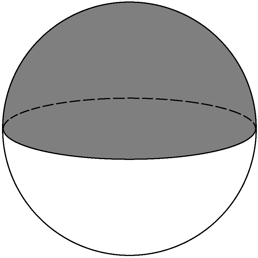
Figure 1: Representation of the two-sphere of emission directions at $r=3M$ in the Schwarzschild spacetime, at which the photon sphere is located. The escape region and the capture region are shown by the grey region and the white region, respectively. The boundary of the two regions is given by an orthodrome.

In a static and spherically symmetric spacetime, the boundary of an escape region associated with a constant-time slice is given by an exact circle. In particular, on the photon sphere in the Schwarzschild spacetime, the boundary of the escape region is given by an orthodrome of the two-sphere (see Fig. 1). One might think that it would be reasonable to define a generalization of the photon sphere as a set of points at which the boundary of the escape region is an orthodrome associated with a constant-time slice, at least for stationary spacetimes. However, in general spacetimes, the boundary of the escape region is not necessarily an exact circle. This leads us to the physical interpretation of our new concepts as described below.

To characterize emission directions $E^{\mu}$ orthogonal to a spacelike vector $n^{\mu}$ in (negations of) Defs. 3.1 and 3.3, the notion of “orthodrome” is useful. In the tangent subspace orthogonal to a unit timelike vector field $T^{\mu}$, an orthodrome is defined as an intersection between a plane containing the origin of the tangent subspace and the two-sphere of emission directions (see circles on the two-spheres in Fig. 2). Note that an orthodrome orthogonal to $n^{\mu}$ represents a set of emission directions $E^{\mu}$ orthogonal to $n^{\mu}$.

The conditions for the ODD and IDD associated with $T^{\mu}$ are now rephrased using the escape and capture cones as follows. On the one hand, the negation of Def. 3.1 is equivalent to that at the spacetime point $p$ outside the ODD, there exists an orthodrome that is entirely included in the escape cone. On the other hand, Def. 3.3 is equivalent to that at a spacetime point $p$ in an IDD, there exists an orthodrome that is entirely included in the capture cone. Note that each of the escape and capture cones can have multiple components. For example, at a point between two distant black holes, there would be two capture cones and one “escape belt”. In the case that each of the escape and capture cones has a single component, a hemisphere is included in the capture cone at a point in the IDD, and a hemisphere is included in the escape cone at a point outside the ODD.

Figure 2 illustrates the situation where each of the escape and capture cones has a single component. Spacetime points can be divided into three classes. In the first class (the left sphere in Fig. 2), there exists an orthodrome which is totally included by the capture cone, and the corresponding point in the spacetime is in the IDD. This point is also in the ODD because the escape cone is included in a hemisphere and it cannot include an orthodrome (a strict proof will be given in Cor. 3.9). In the second class (the center sphere in Fig. 2), there is no orthodrome that is entirely included by the escape region or by the capture region. The corresponding points in the spacetime are in the ODD, but not in the IDD. In the last class (the right sphere in Fig. 2), there exists a hemisphere which is totally included in the escape region. In this case, the corresponding point is not in the ODD as mentioned above. In addition, since the capture cone is included in a hemisphere, this point is not in the IDD (see a strict proof for Cor. 3.9).

In short, any point in the ODD has a small escape cone, and any point not in the ODD has a large escape cone. As for the IDD, any point in the IDD has a large capture cone, and any point not in the IDD has a small capture cone. There is no point such that it is in the ODD and not in the IDD, which will be proved more strictly in Cor. 3.9.

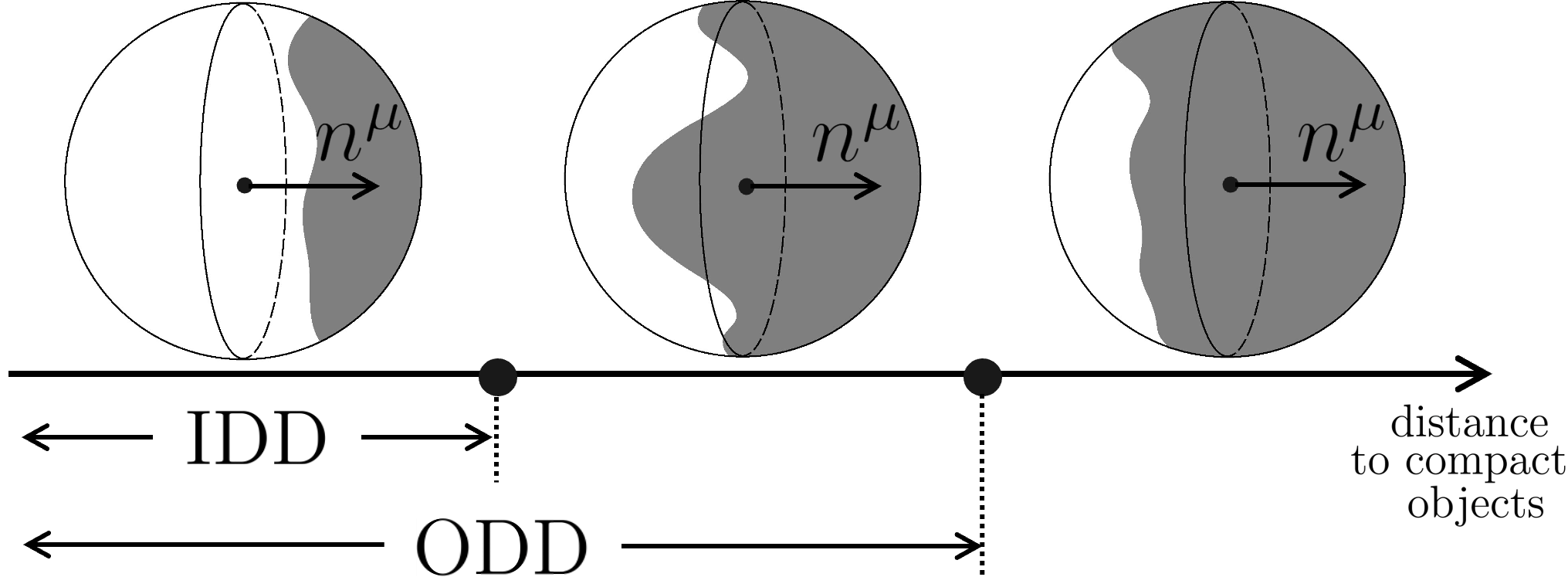
Figure 2: Depiction of two-spheres of emission directions, which represent the escape regions (the grey regions) and the capture regions (the white regions) on three points in a spacetime without symmetry. A vector orthogonal to the plane including the orthodrome corresponds to the spacelike vector $n^{\mu}$ in (negations of) Defs. 3.1 and 3.3. Left sphere: An illustration of the escape and capture regions at a certain point. In this case, this point is both in the ODD and in the IDD. Center sphere: A picture of the escape and capture regions at another point. In other words, all orthodromes intersect the boundary of the two regions. In this case, the point is in the ODD but not in the IDD. Right sphere: An illustration of the escape and capture regions at another point. In this case, the point is not in the ODD nor IDD.

We now present several useful propositions in order to judge whether a given spacetime point is in an ODD/IDD or not. For this purpose, we prove the following Lemma:

Lemma 3.6.

Consider a unit two-sphere and a pair of antipodal points $P$ and $Q$ on that sphere. Let $\gamma$ be any continuous curve that connects $P$ and $Q$, and $\gamma$ includes the two endpoints $P$ and $Q$. Then, any orthodrome on that sphere intersects $\gamma$.

Proof.

In the case that the orthodrome includes the points $P$ and $Q$, it trivially intersects $\gamma$. In the case that the orthodrome does not include $P$ and $Q$, the orthodrome divides the two-sphere into two regions, and the points $P$ and $Q$ are included in different regions because they are antipodal points. Since the curve $\gamma$ continuously connects $P$ and $Q$, it must cross the boundary of the two regions. That is, the orthodrome intersects $\gamma$. ∎

Suppose that a pair of antipodal points are included in a connected component of the capture cone. Then, there exists a curve that connects the two points in the capture cone. From the above Lem. 3.6, any orthodrome crosses that curve, and hence, it cannot be included entirely in the escape cone. This means that the point is in an ODD. For a point at which each of the escape and capture cones is path-connected, we easily see that the reverse is also true and obtain the following:

Theorem 3.7.

If a pair of antipodal points are included in a connected component of the capture cone, the point in the spacetime is in an ODD. In particular, suppose that each of the escape and capture cones is path-connected. Then, a point is in an ODD if and only if the capture cone contains a pair of antipodal points.

Similarly, when a pair of antipodal points are included in a connected component of the escape cone, there exists a curve that connects the two points in the escape cone. Since any orthodrome crosses that curve, it cannot be entirely included in the capture cone. This means that the point is not in an IDD. For a point at which each of the escape and capture cones is path-connected, we see that the reverse also holds.

Theorem 3.8.

If a pair of antipodal points are included in a connected component of the escape cone, the point is not in an IDD. In particular, suppose that each of the escape and capture cones is path-connected. Then, a point is not in an IDD if and only if the escape cone contains a pair of antipodal points.

At a point $p$ in an IDD, an orthodrome is included in the capture cone. This immediately implies the existence of an infinite number of pairs of antipodal points in a connected component of the capture cone. Then, Thm. 3.7 implies that the point $p$ is also in an ODD, and hence, we have the following:

Corollary 3.9.

An IDD is always included in an ODD, as long as they are associated with the same $T^{\mu}$.

We now present the useful criteria to find an ODH and an IDH. For this purpose, we regard the escape and capture cones as mappings from spacetime points. Assuming their continuity, we can find the following:

Proposition 3.10.

Suppose that each of the escape and capture cones has a single component at each spacetime point, and they are continuous mappings with respect to spacetime points. Then, at the ODH, there is an orthodrome that is included in the escape cone except at two or more points, which are on the boundary of the escape and capture cones. Similarly, at the IDH, there is an orthodrome that is entirely included in the capture cone, and furthermore, the orthodrome intersects the boundary of the escape and capture cones at two or more points.

There are several remarks on this Proposition. First, the continuity of the escape and capture cones is guaranteed if the spacetime metric has $C^{2-}$ continuity, and the timelike vector field $T^{\mu}$ is continuous. Here, other than the ODH or the IDH, there might be a surface having the same property for the ODH/IDH mentioned in Prop. 3.10. However, the outermost surface among them can be identified as the ODH/IDH.

3.3 Properties of Outer Dark Domain and Outer Dark Horizon

In this subsection, we provide several properties on the ODD and ODH. First, since all null geodesics in the Minkowski spacetime reach future null infinity, we have the following proposition.

Proposition 3.11.

In the Minkowski spacetime, the ODD and ODH are both absent for any associated timelike vector field $T^{\mu}$.

Proposition 3.11 means that the curved spacetime is essential for the existence of the ODH.

Next, we focus on the spacetimes with black hole(s). For any point $p$ in a black hole, all null geodesics emanating from $p$ do not reach future null infinity by the definition of the black hole. Therefore, $p$ is an element of the ODD. This is summarized as the following theorem:

Theorem 3.12.

In an asymptotically flat spacetime with black hole(s), points in the black hole(s) are also in the ODD for every associated timelike vector field.

Let us discuss the existence of the ODH in spacetimes with black hole(s). To see this, we first show the following lemma.

Lemma 3.13.

Consider a four-dimensional asymptotically flat spacetime in which the metric near future null infinity behaves as Eqs. (2)–(5) with $C^{2-}$ functions using Bondi coordinates. Let a timelike vector $T^{\mu}$ satisfy $T^{\mu}\propto d(u+r)^{\mu}$. We assume that $\Omega_{i}$, which is defined in Eq. (15), is positive. Then, all points $p$ with a sufficiently large $r$ are not in the ODD associated with $T^{\mu}$.

Proof.

We will show that, for all point $p$ with sufficiently large $r$, there exists a tangent vector $n^{\mu}$ orthogonal to $T^{\mu}$, such that all null geodesics which are orthogonal to $n^{\mu}$ at $p$ reach future null infinity. Taking $n^{\mu}=n_{1}^{\mu}:=\left(\partial_{u}\right)^{\mu}-\left(\partial_{r}\right)^{\mu}$ to be an orthogonal vector to $T^{\mu}$, we will show that any null vector $k^{\mu}=\left(\partial_{u}\right)^{\mu}+k^{r}\left(\partial_{r}\right)^{\mu}+k^{I}\left(\partial_{I}\right)^{\mu}$  orthogonal to $n_{1}^{\mu}$ satisfies $k^{r}={{\cal O}\left(r^{-1}\right)}$. By using Eqs. (2), (3), and (5), the orthogonal condition between $n_{1}^{\mu}$ and $k^{\mu}$, that is, $n_{1}^{\mu}k_{\mu}=0$, gives

$$-k^{r}\left(1+{{\cal O}\left(r^{-2}\right)}\right)+k^{I}{{\cal O}\left(r^{0}\right)}+{{\cal O}\left(r^{-1}\right)} = 0$$ (20)

and we have

$$k^{r} = k^{I}{{\cal O}\left(r^{0}\right)}+{{\cal O}\left(r^{-1}\right)}.$$ (21)

Then, a simple calculation gives us

$$0 = k^{\mu}k_{\mu}$$ (22)

$$= k^{I}k^{J}\left(r^{2}\omega_{IJ}+{{\cal O}\left(r^{1}\right)}\right)+k^{I}{{\cal O}\left(r^{0}\right)}-1+{{\cal O}\left(r^{-1}\right)}$$

and we see

$$k^{I} = {{\cal O}\left(r^{-1}\right)}.$$ (23)

With Eq. (21), this shows us

$$k^{r} = {{\cal O}\left(r^{-1}\right)}.$$ (24)

As a consequence, we have $k^{r}={{\cal O}\left(r^{-1}\right)}={{\cal O}\left(r^{-1}\right)}k^{u}$. By Prop. 2.1, null geodesics with $k^{r}={{\cal O}\left(r^{-1}\right)}k^{u}$ at sufficiently large $r$ region reach future null infinity if $\Omega_{i}>0$ holds. Thus, all null geodesics which are orthogonal to $n_{1}^{\mu}$ at $p$ reach future null infinity. Therefore, $p$ is not in the ODD associated with $T^{\mu}$. ∎

Here, Lem. 3.13 does not depend on whether there exist black hole(s) or not. We can also show a higher-dimensional version of Lem. 3.13 in a similar way. Note that in higher dimensions, $\Omega_{i}>0$ is not necessary to show the null geodesics to reach future null infinity Amo:2021gcn ; Amo:2022tcg . Since the same fact also holds for all other theorems, we will not mention higher-dimensional cases, hereinafter.

Now, let us show the existence of the ODH in spacetimes with black hole(s) under the same conditions with Lem. 3.13.

Proposition 3.14.

Consider an asymptotically flat spacetime with black hole(s) under the assumptions in Lem. 3.13. The ODH associated with $T^{\mu}$ is not empty, and not connected to future null infinity.

Proof.

Let the region of the ODD be denoted by $S$. Then, $S$ is not empty by Thm. 3.12. Due to Lem. 3.13, a region sufficiently close to future null infinity is a subset of $\mathcal{M}\backslash S$. Therefore, the ODH is not empty by Def. 3.2, and not connected to future null infinity. ∎

This proposition is supporting evidence for the ODH to serve as an indicator for a strong gravity region.

3.4 Properties of Inner Dark Domain and Inner Dark Horizon

In this subsection, we provide several properties on the IDD and IDH. In the same way to the proofs for Prop. 3.11 and Thm. 3.12, we can easily show the following statements.

Proposition 3.15.

In the Minkowski spacetime, the IDD and IDH are both absent for any associated timelike vector field $T^{\mu}$.

Theorem 3.16.

In an asymptotically flat spacetime with black hole(s), points in the black hole are elements of the IDD for any associated timelike vector field $T^{\mu}$.

Proposition 3.15 means that curved spacetimes are essential for the existence of the IDD and IDH. Meanwhile, Thm. 3.16 guarantees the existence of the IDD in spacetimes with black hole(s).

To show the existence of the IDH in spacetimes with black hole(s), the following lemma is essential, which can easily be verified by using Cor. 3.9 and Lem. 3.13.

Lemma 3.17.

Under the assumptions in Lem. 3.13, all points $p$ with sufficiently large $r$ are not in the IDD associated with $T^{\mu}$.

One expects that the IDH serves as an indicator for the existence of a strong gravity region. This is indeed correct as the following proposition.

Proposition 3.18.

Consider an asymptotically flat spacetime with black hole(s) under the assumptions in Lem. 3.13. The IDH associated with $T^{\mu}$ is not empty, and not connected to future null infinity.

Proof.

The IDD $S$ is not empty by Thm. 3.16. In addition, a region sufficiently close to future null infinity is a subset of $\mathcal{M}\backslash S$ due to Lem. 3.17. Therefore, the IDH is not empty, and not connected to future null infinity by Def. 3.4. ∎

Finally, let us prove that the ODH coincides with the IDH in a spherically symmetric spacetime for the spherically symmetric unit timelike vector field $T^{\mu}$:

Theorem 3.19.

Consider an asymptotically flat, spherically symmetric spacetime. Let $x^{I}$ be the angular coordinates. We adopt the timelike vector field $T^{\mu}$ to be the spherically symmetric one that satisfies $T^{\mu}(dx^{I})_{\mu}=0$. Then, the ODH associated with $T^{\mu}$ coincides with the IDH associated with $T^{\mu}$.

Proof.

If the ODD and IDD coincide with each other, the ODH and IDH also coincide with each other. Here, the IDD is a subset of the ODD by Cor. 3.9. Therefore, the task here is to show that the ODD is a subset of the IDD.

Let a point $p$ be in the ODD. By the definition of the ODD, for all spacelike vectors $n^{\mu}$ orthogonal to $T^{\mu}$, there exists a null geodesic which emanates from $p$, whose tangent vector $k^{\mu}$ is orthogonal to $n^{\mu}$ at $p$, such that it will not reach future null infinity. We now adopt $n^{\mu}$ as the one satisfying $n^{I}=0$. Due to the spherical symmetry of the spacetime, all null geodesics with the tangent vector $k^{\mu}$ satisfying $k^{\mu}n_{\mu}=0$ emanating from $p$ will not reach future null infinity. Then, $p$ satisfies the condition of being in the IDD. ∎

4 Explicit example I: static and spherically symmetric spacetimes

This section concerns a static, spherically symmetric and asymptotically flat spacetime with the metric,

$$ds^{2} = -f(r)dt^{2}+g(r)dr^{2}+r^{2}\left(d\theta^{2}+\sin^{2}\theta d\phi^{2}\right).$$ (25)

Here, the fall-off condition for the asymptotical flatness is written as

$$f(r)=1+{{\cal O}\left(r^{-1}\right)},\quad g(r)=1+{{\cal O}\left(r^{-1}\right)}.$$ (26)

In this section, we adopt the timelike unit vector field $T^{\mu}$ as $T^{\mu}=(\partial_{t})^{\mu}/\sqrt{f(r)}$. In other words, we consider the dark domains and the dark horizons associated with $t-$constant hypersurfaces $\Sigma_{t}$, and omit the phrase “associated with $T^{\mu}$” or “associated with $\Sigma_{t}$” until the end of this section. Due to Thm. 3.19, the ODD and IDD coincide with each other, and the same statement holds also for the ODH and IDH. For this reason, we just call them the dark domain and the dark horizon, respectively.

Assuming the Einstein equation, we have

$$f(r)\ =\ \frac{1}{g(r)}\ =\ 1-\frac{2M}{r}$$ (27)

in the vacuum region. In such a situation, we have a clear relation of the dark horizon and photon sphere:

Theorem 4.1.

Consider a static, spherically symmetric and asymptotically flat spacetime Eq. (25) in which there exists $r_{\rm v}$ satisfying $r_{\rm v}<3M$, such that the region $r\geq r_{\rm v}$ is vacuum, where $M$ is the ADM mass. And we assume that the Einstein equation holds in $r\geq r_{\rm v}$. Then, the hypersurface $r=3M$ is the dark horizon. In particular, in the Schwarzschild spacetime, the photon sphere coincides with the dark horizon.

Proof.

Due to Birkhoff’s theorem, the region for $r\geq r_{\rm v}$ is the Schwarzschild spacetime. Firstly, let us show that a point $p$ with $r>3M$ is not in the dark domain. In the Schwarzschild spacetime, for any point in the region $r>3M$, for all spacelike vectors $n^{\mu}$ orthogonal to $T^{\mu}$, there exists a null geodesic whose tangent vector is orthogonal to both $n^{\mu}$ and $\left(\partial_{r}\right)^{\mu}$. This null geodesic cannot enter the region $r\leq 3M$, and will reach future null infinity as in the Schwarzschild spacetime. Therefore, $p$ is not in the dark domain.

Secondly, let us show that a point $p$ with $r_{\rm v}<r<3M$ is in the dark domain. Taking $n^{\mu}=(\partial_{r})^{\mu}$ to see that $p$ is in the dark domain, we will prove that any null geodesic which emanates from $p$ and is orthogonal to $n^{\mu}$ at $p$ does not reach future null infinity. In the region $r>r_{\rm v}$, the radial coordinate will decrease on the null geodesic for a while and this null geodesic reaches $r=r_{\rm v}$ as in the Schwarzschild spacetime. Now, we classify the situations into two cases. In one case, the null geodesic will not come back to the region $r>r_{\rm v}$ again. In this case, the null geodesic does not reach future null infinity. In the other case, the null geodesic has the periapsis, i.e., a turning point $q$ with respect to the radial coordinate $r$ (see Fig. 3). By virtue of the staticity and spherical symmetry, the orbit is symmetric with respect to $q$, namely, if we consider the equatorial plane $\theta=\pi/2$ in the ordinary $(t,r,\theta,\phi)$ coordinates, the orbit is given by $r=r(\phi)$ with the property $r(2\phi_{q}-\phi)=r(\phi)$, where $\phi_{q}$ is the value of $\phi$ at the point $q$. This means that there exists a point $p^{\prime}$ such that the tangent vector of the null geodesic at $p^{\prime}$ is normal to $n^{\mu}$ similarly to the emission point $p$ (see Fig. 3). The orbit of the null geodesics after $p^{\prime}$ is the same as the one after $p$ except that the initial angular position $\phi_{p}$ is replaced by $\phi_{p^{\prime}}$. To be more specific, the orbit has the periodicity $r(\phi-n(\phi_{p^{\prime}}-\phi_{p}))=r(\phi)$ with the integer $n$. This means that the radial oscillation will be repeated infinite times, and thus, the null geodesic does not reach future null infinity. Summarizing the above two cases, any point $p$ with $r<r_{\rm v}$ is in the dark domain. Therefore, $r=3M$ is the dark horizon. ∎

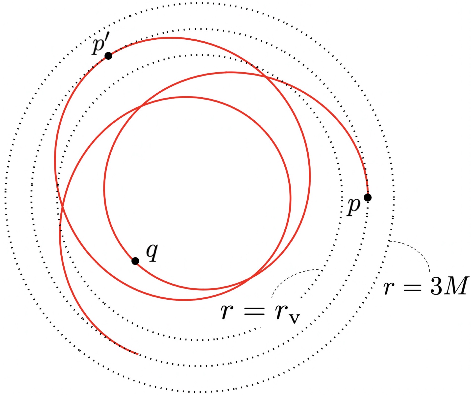
Figure 3: An illustration of $p$, $q$, and $p^{\prime}$ in the proof of Thm. 4.1. The red solid curve represents the orbit of the null geodesic. The point $q$ is the periapsis, and $p$ and $p^{\prime}$ are the apoapses.

As a preparation for the discussion on the dark horizon in more general cases where the metric is given in the form of Eq. (25), let us probe null geodesics in the spacetime by utilizing the discussion for null geodesic to reach future null infinity Ogasawara:2020frt ; Carter:1968rr ; Walker:1970un . The non-zero components of the Killing tensor $K_{\mu\nu}$ are

$$K_{\theta\theta}=r^{4},\qquad K_{\phi\phi}=r^{4}\sin^{2}\theta.$$ (28)

Here, the impact parameter $b:=-k_{\phi}/k_{t}$ and dimensionless Carter’s constant $q:=(K_{\mu\nu}k^{\mu}k^{\nu}-b^{2})/k_{t}^{2}$ are both conserved along the geodesic. In the spherically symmetric spacetimes, without loss of generality, we can restrict our considerations to the case with $b\geq 0$ and $q=0$. This corresponds to the case that the photon propagates on the equatorial plane in the $+\phi$ direction.

Let us see that there exists a forbidden region of the impact parameter depending on the radial coordinate. The geodesic equation for $r$ is given by

$$r^{4}r^{\prime 2}=R,$$ (29)

where $R:=r^{2}\left(r^{2}-fb^{2}\right)/(fg)$ is non-negative and the prime is the derivative with respect to the affine parameter. Let us restrict our attention to the region $f>0$ and $g>0$ because we are interested in the static spacetimes. Then, from the non-negativity of $R$, we see

$$|b|\leq B(r),$$ (30)

where $B(r)$ is defined as

$$B(r):=\frac{r}{\sqrt{f(r)}},$$ (31)

and Eq. (29) shows that the equality in Eq. (30) holds for $r^{\prime}=0$. It is easy to see

$$\left.\frac{dR}{dr}\right|_{b=B(r)}=\frac{2r^{3}}{f^{1/2}(r)g(r)}\frac{dB(r)}{dr},$$ (32)

and then, the derivative of Eq. (29) gives us

$$\left.r^{\prime\prime}\right|_{r^{\prime}=0}=\frac{1}{2r^{4}}\left.\frac{dR}{dr}\right|_{b=B(r)}=\frac{1}{rf^{1/2}(r)g(r)}\frac{dB}{dr}.$$ (33)

Thus, we see that the sign of $\left.r^{\prime\prime}\right|_{r^{\prime}=0}$ and that of $dB/dr$ coincide with each other outside the event horizon, which is consistent with Eq. (31), that is, the allowed region is below the curve of $b=B(r)$ in Fig. 4. In particular, $dB/dr=0$ is necessary and sufficient condition for $\left.r^{\prime\prime}\right|_{r^{\prime}=0}=0$ determining the locus of the photon sphere, outside the event horizon. Using this fact, we can examine whether null geodesics reach future null infinity or not in a static, spherically symmetric and asymptotically flat spacetime. Since $b$ is conserved along null geodesics, the behavior of the null geodesics is determined by a $b-$constant line and the shape of $B(r)$ on the $(r,b)$-plane just like the discussion based on the effective potential in the classical mechanics. For the discussion that appears soon, we write down $dB(r)/dr$ explicitly as

$$\frac{dB}{dr}=\frac{2f(r)-rdf/dr(r)}{2f^{3/2}(r)}.$$ (34)

Next, to show the relation between the dark horizon and the photon sphere, we classify the photon sphere into two types.

Definition 4.2 (visible and invisible photon sphere)

Consider a static, spherically symmetric and asymptotically flat spacetime with the metric of Eq. (25). We call a photon sphere at $r=r_{0}$ the visible photon sphere when $B(r)$ takes the minimal value at $r=r_{0}$ and for all $\tilde{r}_{0}>r_{0}$, $B(\tilde{r}_{0})\neq B(r_{0})$. We also define the invisible photon sphere as a photon sphere which is not a visible photon sphere.

The null geodesics passing slightly outside of the visible photon sphere with $r^{\prime}=0$ reach future null infinity, while the null geodesics passing slightly outside of the invisible photon sphere with $r^{\prime}=0$ do not reach future null infinity, from which their names stem. This is understood from the shape of $B(r)$ as shown in Fig. 4. In particular, the photon sphere at $r=3M$ in the Schwarzschild spacetime is a visible photon sphere.

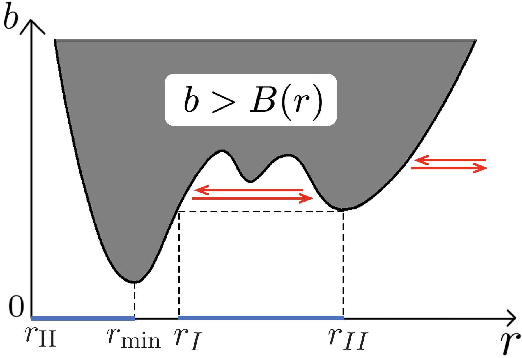
Figure 4: This is an example having five photon spheres. The shaded region $b>B(r)$ is the forbidden region. Null geodesics, which are described as $b-$constant lines, are reflected after they reach $b=B(r)$ (see red arrows). The intervals $[r_{\rm H},r_{\rm min}]$ and $[r_{I},r_{II}]$ correspond to the dark domain, which are indicated by blue lines. Here, $r_{\rm H}$, $r_{I}$ and $r_{II}$ denote the horizon radius, the second outermost dark horizon and the outermost dark horizon, respectively. In this spacetime, the dark horizon composes of three connected components.

As for the relation between the visible photon sphere and the outermost photon sphere, we have the following proposition.

Proposition 4.3.

Consider a static, spherically symmetric and asymptotically flat spacetime with the metric of Eq. (25). The outermost photon sphere is a visible photon sphere.

Proof.

Equations (26) and (34) give us $dB/dr>0$ for sufficiently large $r$. In addition, photon spheres are characterized by the condition $dB/dr=0$. Then, by the continuity of $dB/dr$, the outermost photon sphere is the visible photon sphere. ∎

Next, we discuss the dark domain in static, spherically symmetric and asymptotically flat spacetimes.

Lemma 4.4.

Consider a static, spherically symmetric and asymptotically flat spacetime with the metric of Eq. (25). A point $(t_{0},r_{0},\theta_{0},\phi_{0})$ is in the dark domain if and only if $dB/dr(r_{0})=0$ holds or there exists $\tilde{r}_{0}>r_{0}$ such that $B(r_{0})=B(\tilde{r}_{0})$.

The above lemma comes from the fact that the dark domain is specified by the so-called bounded orbit. The range of $r$ of the dark domain depends on the shape of $B(r)$. In an example such as Fig. 4, the dark domain spreads over the intervals $[r_{\rm H},r_{\rm min}]$ and $[r_{I},r_{II}]$. For those who are interested in a strict proof, see App. A.

It is easy to guess that a dark horizon is a generalization of the visible photon sphere. This is indeed true and summarized as the following theorem.

Theorem 4.5.

Consider a static, spherically symmetric and asymptotically flat spacetime with the metric of Eq. (25). A visible photon sphere is a dark horizon. In particular, the outermost photon sphere coincides with the outermost dark horizon.

The holding of this theorem is seen as follows. Since $B(r)$ has a local minimum at the visible photon sphere, say $r=r_{1}$, and there is the region composed of the bound orbits of null geodesics for $r<r_{1}$. This means that the point with $r=r_{1}-\epsilon$ for sufficiently small $\epsilon(>0)$ is included in the dark domain, and the point with $r=r_{1}+\epsilon$ is not included in the dark domain. Thus, $r=r_{1}$ is the dark horizon. It is trivial that the outermost photon sphere is the outermost dark horizon.

Here, Thm. 4.1 can also be trivially proven from Thm. 4.5 because a spacetime in Thm. 4.1 has a visible photon sphere at $r=3M$ by Birkhoff’s theorem. Theorem 4.5 guarantees that the dark horizon includes a generalization of the visible photon sphere. Note that there are photon spheres which are not dark horizons. For example, stable photon spheres, on which $B(r)$ is maximal, are not dark horizons.

It should be also noted that there exist dark horizons which are not photon spheres. In a spacetime with $B(r)$ of Fig. 4, there are two connected dark domains. The inner boundary of the outer component of the dark domain is a dark horizon, but not a photon sphere. Let us discuss the physical meaning of this dark horizon. As shown in Fig. 4, we express the radial coordinate of this dark horizon as $r_{I}$, and that of the outermost dark horizon as $r_{II}$. Then, let us consider the observation of photons emitted from this region. For a distant observer, the image of the observed region can be regarded as a series of concentric circles, and each circle is specified by the angle $\vartheta$ from the center of the image. Here, the angle $\vartheta$ is a monotonically increasing function of the impact parameter $b$, and $\vartheta=0$ corresponds to $b=0$. When one regards the minimum radial coordinate for each null geodesic as a function of $b$, it has a discontinuity at $b_{c}:=B(r_{I})=B(r_{II})$, and hence, the observable region changes discontinuously at a certain angle $\vartheta_{c}$ corresponding to the impact parameter $b_{c}$. Namely, we observe the region $r>r_{II}$ for $\vartheta=\vartheta_{c}+0$, while we catch signals from the region $r\geq r_{I}$ for $\vartheta=\vartheta_{c}-0$. This gives the physical meaning of the dark horizon that is not the photon sphere.

5 Explicit example II: Vaidya spacetime

In this section, as an example of dynamical spacetimes, we investigate the dark horizon in the Vaidya spacetime. The Vaidya spacetime has two classes depending on the directions of the flow—ingoing and outgoing Vaidya spacetimes. Their metrics are written as

$$ds^{2}=-\left(1-\frac{2M(v)}{r}\right)dv^{2}+2dvdr+r^{2}\left(d\theta^{2}+\sin^{2}\theta d\phi^{2}\right),$$ (35)

and

$$ds^{2}=-\left(1-\frac{2M(u)}{r}\right)du^{2}-2dudr+r^{2}\left(d\theta^{2}+\sin^{2}\theta d\phi^{2}\right),$$ (36)

respectively, where $v$ and $u$ are the advanced and retarded times, respectively. We focus our attention to the domain where $r>2M(v)$ and $r>2M(u)$ hold, and adopt the timelike vector field $T^{\mu}$ as proportional to $(\partial_{v})^{\mu}$ and $(\partial_{u})^{\mu}$ in the ingoing and outgoing Vaidya spacetimes, respectively. Due to Thm. 3.19, the ODH and IDH associated with the same unit time vector field $T^{\mu}$ coincide with each other. In what follows, we just call the ODH and IDH the dark horizon, and do not write “associated with $T^{\mu}$” in this section.

In Ref. Koga:2022dsu , the shadow edge orbits in the Vaidya spacetime were discussed for an idealized situation in which the observer and the light source are supposed to be located at future null infinity and past null infinity, respectively. In this sense, the authors of Ref. Koga:2022dsu defined the dynamical photon sphere as the boundary of the set of null geodesics connecting future and past null infinity, and explicitly calculated the time-dependence of the dynamical photon sphere. To compare the dark horizon with the dynamical photon sphere, let us examine the dark horizon in the same setup.

In the case with the ingoing Vaidya spacetime, we use the same mass function as that in Ref. Koga:2022dsu :

$$M(v)=\left\{\begin{array}[]{cc}1&(v\leq 0);\\ 2-\cos\left(\dfrac{v}{v_{\rm f}}\pi\right)&(0<v\leq v_{\rm f});\\ 3&(v>v_{\rm f}),\end{array}\right.$$ (37)

with $v_{\rm f}=100$. In order to specify the position of the dark horizon at each $v$, we numerically solved the null geodesic equation with the initial condition that corresponds to $r=r_{0}$ and $k^{r}=0$, where $k^{\mu}$ is a tangent vector of the null geodesic. By changing the initial values of $r_{0}$, we specified the radius of the dark horizon $r_{\rm DH}$ such that the null geodesic enters the black hole region for $r_{0}<r_{\rm DH}$ and escapes to infinity for $r_{\rm DH}<r_{0}$. The dynamical photon sphere is also obtained numerically in the same way as Ref. Koga:2022dsu .

Figure 5 shows the radii of the dark horizon, the dynamical photon sphere and the graph $r=3M(v)$. To see the difference between the dark horizon and the dynamical photon sphere, consider two sets of null geodesics—ones corresponding to the dark horizon and ones corresponding to the dynamical photon sphere. The null geodesics emitted from the dark horizon initially have $k^{r}=0$. By contrast, from the behavior of the dynamical photon sphere depicted in the Fig. 5, the null geodesics corresponding to the dynamical photon sphere has $k^{r}>0$ because the null geodesics are included in the dynamical photon sphere, whose area increases with time. This is the reason why the dark horizon is located outside the dynamical photon sphere, shown in Fig. 5. This is a consequence of the assumption that the light sources are located at past null infinity in this case. Here, both sets of null geodesics describe the boundary of null geodesics which reach future null infinity or not, but the locations of the light sources are different.

Figure 5: Comparison between the dark horizon (gray dots) and the dynamical photon sphere (red curve) in the ingoing Vaidya spacetime with the metric Eqs. (35) and (37). The blue dashed curve denotes $r=3M(v)$.

Similarly, in the case of the outgoing Vaidya spacetime, we use the mass function as follows:

$$M(u)=\left\{\begin{array}[]{cc}3&(u\leq 0);\\ 2+\cos\left(\dfrac{u}{u_{\rm f}}\pi\right)&(0<u\leq u_{\rm f});\\ 1&(u>u_{\rm f}),\end{array}\right.$$ (38)

with $u_{\rm f}=100$. Figure 6 shows the dark horizon, the dynamical photon sphere and the graph $r=3M(u)$. One can see that the dark horizon is located inside of the dynamical photon sphere. The reason is interpreted as follows. The null geodesics that correspond to the edge of the escape cone at the dark horizon has the vanishing radial component of the tangent vector, $k^{r}=0$. By contrast, the plot of the dynamical photon sphere in the Fig. 6 tells us that the null geodesics corresponding to the dynamical photon sphere direct inward because the null geodesics are included in the dynamical photon sphere, whose area decreases with time. This gives us the reason why the dark horizon is located inside of the dynamical photon sphere, shown in Fig. 6. This is a consequence of the assumption that the light sources are located at past null infinity in this case. Here, both sets of null geodesics describe the boundary of null geodesics which reach future null infinity or not, but the locations of the light sources are different.

Figure 6: Comparison between the dark horizon (gray dots) and the dynamical photon sphere (red curve) in the outgoing Vaidya spacetime with the metric Eqs. (36) and  (38). The blue dashed curve corresponds to $r=3M(u)$.

6 Explicit example III: Kerr spacetime

In this section, we study the dark horizons in the Kerr spacetime as a simple model of typical black holes in our Universe. To be specific, we consider the ODH and IDH associated with a timeslice $\Sigma_{t}$ of the Boyer-Lindquist coordinates $(t,r,\theta,\phi)$. This section is organized as follows. In subsection 6.1, we show basic properties of null geodesics in the Kerr spacetime. In subsection 6.2, the ODH and IDH on the rotation axis is considered. In subsections 6.3 and 6.4, we investigate the ODH and IDH in the Kerr spacetime, respectively.

6.1 Preparation

In this subsection, we conduct several calculations as a preparation for the depiction of the shapes of the ODH and IDH in the Kerr spacetime. The metric of the Kerr spacetime is given by

$$ds^{2} = -\frac{\Sigma\Delta}{A}dt^{2}+\frac{\Sigma}{\Delta}dr^{2}+\Sigma d\theta^{2}+\frac{A}{\Sigma}\sin^{2}\theta\left(d\varphi-\frac{2Mar}{A}dt\right)^{2},$$ (39)

where $\Sigma$, $\Delta$, and $A$ are defined as

$$\Sigma:=r^{2}+a^{2}\cos^{2}\theta,~{}~{}\Delta:=r^{2}-2Mr+a^{2},~{}~{}A:=\left(r^{2}+a^{2}\right)^{2}-a^{2}\Delta\sin^{2}\theta.$$ (40)

Here, $M$ is the ADM mass and $a$ is the rotation parameter that is related to the ADM angular momentum as $J=Ma$. We also sometimes use the dimensionless rotation parameter $a_{*}=a/M$ to specify the solution. Below, the black hole spacetime with a nondegenerate event horizon, $0<|a_{*}|<1$, is considered (see Sec. 4 for the case of $a_{*}=0$). The event and Cauchy horizons are located at $r=r_{\rm H}^{+}$ and $r=r_{\rm H}^{-}$, respectively, where

$$r_{\rm H}^{\pm}\,=\,M\pm\sqrt{M^{2}-a^{2}},$$ (41)

and we shall limit our attention to the region outside the event horizon, $r>r_{\rm H}^{+}$. Let us introduce the tetrad in the Kerr spacetime as follows:

$$\left(e_{0}\right)^{\mu} = \left(\sqrt{\frac{A}{\Delta\Sigma}},0,0,\frac{2Mar}{\sqrt{A\Delta\Sigma}}\right),$$ (42)

$$\left(e_{1}\right)^{\mu} = \left(0,\sqrt{\frac{\Delta}{\Sigma}},0,0\right),$$ (43)

$$\left(e_{2}\right)^{\mu} = \left(0,0,\frac{1}{\sqrt{\Sigma}},0\right),$$ (44)

$$\left(e_{3}\right)^{\mu} = \left(0,0,0,\sqrt{\frac{\Sigma}{A}}\frac{1}{\sin\theta}\right).$$ (45)

Here, $\left(e_{0}\right)^{\mu}$ is orthogonal to the $t$-constant slice $\Sigma_{t}$ of the Boyer-Lindquist coordinates. The ODD, ODH, IDD, and IDH associated with $\Sigma_{t}$ in the Def. 3.5 are equivalent to those associated with $T^{\mu}=\left(e_{0}\right)^{\mu}$ in the Defs. 3.1, 3.2, 3.3, and 3.4. The timelike vector field $\left(e_{0}\right)^{\mu}$ is equivalent to the four-vector fields of the zero-angular-momentum observers (ZAMOs) (e.g. Frolov:1998 ). The tetrad basis of Eqs. (42)–(45) gives a natural frame associated with ZAMOs, and we consider the escape/capture cones in this ZAMO frame. We show an illustrative figure for the spatial vectors $\left(e_{1}\right)^{\mu}$, $\left(e_{2}\right)^{\mu}$, and $\left(e_{3}\right)^{\mu}$ in the left panel of Fig. 7.

Figure 7: The spatial vectors of the tetrad basis and the emission direction vector. Left panel: The configuration of $\mathbf{e}_{1}$, $\mathbf{e}_{2}$, and $\mathbf{e}_{3}$ at some spatial point on a $t$-constant hypersurface, where $\mathbf{e}_{1}$, $\mathbf{e}_{2}$, and $\mathbf{e}_{3}$ correspond to Eqs. (43), (44), and (45), respectively. The black sphere is the event horizon, and the larger sphere indicates an $r$-constant surface. At each point, $\mathbf{e}_{1}$, $\mathbf{e}_{2}$, and $\mathbf{e}_{3}$ are parallel to $\partial_{r}$, $\partial_{\theta}$, and $\partial_{\phi}$, respectively. Right panel: The definition of $\xi$ and $\eta$ to parametrize the emission direction given in Eq. (46). Here, $\mathbf{E}$ indicates the emission direction vector given by Eq. (19) [the spatial part of Eq. (46)].

At each point $p$ of the Kerr spacetime, we consider the (initial) null tangent vector $k^{\mu}$ of a null geodesic that corresponds to a photon emitted from the point $p$. Adopting the normalization $k^{\mu}\left(e_{0}\right)_{\mu}=-1$ , the initial null tangent vector $k^{\mu}$ is expressed in the form of

$$k^{\mu} = \left(e_{0}\right)^{\mu}+\cos\xi\left(e_{1}\right)^{\mu}+\sin\xi\sin\eta\left(e_{2}\right)^{\mu}+\sin\xi\cos\eta\left(e_{3}\right)^{\mu},$$ (46)

where $0\leq\xi\leq\pi$ and $-\pi\leq\eta<\pi$. See the illustration for the definition of $\xi$ and $\eta$ in the right panel of Fig. 7. Then, at each point $p$, the covariant components $k_{t}$ and $k_{\phi}$ are written down as

$$\left.k_{t}\right|_{p} = -\sqrt{\frac{\Delta\Sigma}{A}}-\frac{2Mar\sin\theta\sin\xi\cos\eta}{\sqrt{A\Sigma}},$$ (47)

$$\left.k_{\phi}\right|_{p} = \sqrt{\frac{A}{\Sigma}}\sin\theta\sin\xi\cos\eta,$$ (48)

where the values of $r$ and $\theta$ at the point $p$ must be used in these equations. After the emission, the motion of the photon follows the null geodesic. In a Kerr spacetime, each null geodesic possesses the conserved quantities, the energy $E$, the angular momentum $L$, and Carter’s constant $Q$ Carter:1968rr (we follow the notation of Ref. Ogasawara:2020frt for Carter’s constant). Their values are determined by the initial condition (i.e., the information at the point $p$), and for the energy and angular momentum, we have $E=\left.-k_{t}\right|_{p}$ and $L=\left.k_{\phi}\right|_{p}$, respectively. The impact parameter $b$ is defined by $b:=L/E$, and its value becomes

$$b\,=\,\left.-\frac{k_{\phi}}{k_{t}}\right|_{p}=\frac{A\sin\theta\sin\xi\cos\eta}{\sqrt{\Delta}\Sigma+2Mar\sin\theta\sin\xi\cos\eta}.$$ (49)

In addition, we introduce the dimensionless Carter’s constant $q=Q/E^{2}$, and the values of $q$ and $b$ satisfy

$$q+(b-a)^{2} = \frac{A\sin^{2}\xi\sin^{2}\eta+\left[\left(r^{2}+a^{2}\right)\sin\xi\cos\eta-a\sqrt{\Delta}\sin\theta\right]^{2}}{\left(\sqrt{\Delta}+2Mar\sin\theta\sin\xi\cos\eta/\Sigma\right)^{2}}.$$ (50)

Eliminating $\eta$ from Eqs. (49) and (50), one has

$$\sin^{2}\xi\,=\,\frac{F(b,q)\Delta}{(A-2Mabr)^{2}},$$ (51)

where

$$F(b,q):=A\left(q+a^{2}\cos^{2}\theta\right)+b^{2}\left[r^{4}+a^{2}\cos^{2}\theta(\Delta-a^{2})\right].$$ (52)

From Eq. (51), it is found that the value of $F(b,q)$ must be nonnegative, that is, the impact parameter $b$ and the dimensionless Carter’s constant $q$ can only take values such that $F(b,q)\geq 0$ is satisfied. Taking the square root of Eq. (51) and substituting it into Eq. (49), we have

$$\sin\xi = \frac{\sqrt{F(b,q)\Delta}}{|A-2Mabr|},$$ (53a)

$$\cos\eta = \mathrm{sgn}(A-2Mabr)\frac{b\Sigma}{\sin\theta\sqrt{F(b,q)}}.$$ (53b)

Next, let us discuss the relation between $\xi$ and $\eta$ on the boundary of the escape/capture cones. It is known that the null geodesics corresponding to the boundary of the escape cone neither reach future null infinity nor fall into the black hole. These null geodesics asymptote to the spherical orbits around the black hole with specific values of $b$ and $q$, which are called the “spherical photon orbits” Teo:2020sey . To discuss the null geodesics which correspond to the boundary of the escape cone, let us look at the relation between $b$ and $q$ for the spherical photon orbits.

Along the null geodesic, the following first-order differential equation holds Carter:1968rr :

$$\Sigma^{2}r^{\prime 2}=R,$$ (54)

where

$$R:=\left[E\left(r^{2}+a^{2}\right)-La\right]^{2}-\Delta\left[Q+(L-aE)^{2}\right].$$ (55)

A spherical photon orbit with the radius $r_{s}$ satisfies $R|_{r=r_{s}}=0$ and $dR/dr|_{r=r_{s}}=0$, and these conditions are rewritten as

$$b = -\frac{r_{s}^{3}-3Mr_{s}^{2}+a^{2}r_{s}+Ma^{2}}{a(r_{s}-M)},$$ (56)

$$q = -\frac{r_{s}^{3}\left(r_{s}^{3}-6Mr_{s}^{2}+9M^{2}r_{s}-4a^{2}M\right)}{a^{2}\left(r_{s}-M\right)^{2}}.$$ (57)

Equations (56) and (57) give the relation between $b$ and $q$ via a parameter $r_{s}$ that is satisfied by various spherical photon orbits.

Next, consider null geodesics asymptoting to spherical photon orbits in the future ($t\to\infty$). These null geodesics correspond to the boundary of the escape cone at a point on these null geodesics. Since $b$ and $q$ of these null geodesics are the same as those of corresponding spherical photon orbits, the same relation of Eqs. (56) and (57) holds. By substituting Eqs. (56) and (57) into Eqs. (53a) and (53b), we obtain the relation between $\sin\xi$ and $\cos\eta$ as parametrized by $r_{s}$, and this relation gives the boundary of the escape cone. However, since two values of $\xi$ give the same $\sin\xi$ in the range $0\leq\xi\leq\pi$, the obtained relation between $\xi$ and $\eta$ includes both the emission directions of photons that asymptote to the spherical photon orbits in the future ($t\to\infty$) and in the past ($t\to-\infty$). Therefore, we must select an appropriate boundary to specify the real escape cone. This can be done by several criteria:

• The structures of the escape cones for a Schwarzschild spacetime are well known, and the escape cones change smoothly as the value of $a_{*}$ is increased;

• The escape cone is a smooth mapping with respect to the spatial positions;

• The boundary of the escape/capture cones must be smooth on the two-sphere of emission directions.

We have found that the formula of $\cos\xi$ that satisfies the above requirements is given by

$$\cos\xi\ =\ \mathrm{sgn}(r_{s}-r)\sqrt{1-\frac{F(b,q)\Delta}{(A-2Mabr)^{2}}}.$$ (58)

In fact, the function in the square root of Eq. (58) has the factor $(r_{s}-r)^{2}$, and hence, Eq. (58) gives an analytic formula with respect to $r_{s}$ for any fixed $r$ and $\theta$. The explicit formula is shown as Eq. (68b) with Eq. (69) in App. B.

Figure 8: The boundaries of the escape and capture cones projected onto the plane spanned by $\mathbf{e}_{3}$ and $\mathbf{e}_{1}$ for $r/M=1.142$, $1.145$, $1.15$, $1.16$, $1.2$, $1.3$, $1.7$, $2.3$, $3.0$, $4.0$, $5.0$, $6.5$, and $10.0$ in the equatorial plane $\theta=\pi/2$ for a Kerr black hole with $a_{*}=0.99$. The upper region of each curve is the escape cone, while the lower region is the capture cone.

Here, we present examples of the boundaries of the escape and capture cones. For this purpose, we consider the projection of the two-sphere of emission directions onto the plane spanned by $\mathbf{e}_{1}$ and $\mathbf{e}_{3}$. In other words, we consider a “side view” of the two-sphere as seen from a distant position with $\xi=\eta=\pi/2$ in the tangent subspace. Then, the two-sphere is projected to a unit disk, and the boundary of the escape and capture cones becomes a curve that has the endpoints on the unit circle due to the symmetry in the transformation $\eta\to-\eta$. Figure 8 presents the projected boundary of the escape and capture cones for various $r$ values on the equatorial plane $\theta=\pi/2$ for $a_{*}=0.99$. The upper region of each curve is the escape cone, while the lower region is the capture cone. Due to the effect of dragging into rotation of the Kerr black hole, the escape cone tends to be directed in the $\mathbf{e}_{3}$ direction.

We point out important properties of the curve of the projected boundary of the escape and capture cones. Let us introduce the Cartesian coordinates $(x,y)$ on the two-dimensional plane defined by $\partial_{x}=\mathbf{e}_{3}$ and $\partial_{y}=\mathbf{e}_{1}$. The origin of the coordinates is set so that the projected two-sphere of emission direction is given by $x^{2}+y^{2}\leq 1$. Note that $\left(\xi,\eta\right)=\left(\pi/2,\pm\pi/2\right)$ are both projected to the origin. The curve of the projected boundary can be expressed as $y=y(x)$. Then, as proved in App. B, it is possible to show the inequalities

$$\frac{dy}{dx}\,\leq\,0,$$ (59)

and

$$\frac{d^{2}y}{dx^{2}}\,\leq\,0,$$ (60)

where equalities hold on and only on the rotation axis. Denoting the two endpoints of the projected boundary of the escape and capture cones as $(\xi,\eta)=(\xi_{+},0)$ and $(\xi_{-},\pi)$, the first inequality of Eq. (59) indicates that $\xi_{+}\geq\xi_{-}$ always holds for $a_{*}>0$. The second inequality of Eq. (60) means that the curve of the projected boundary is convex upward (i.e. concave downward). This property will be used in figuring out the ODH and IDH.

For a later convenience, let us examine the behavior of a null geodesic whose tangent vector $k^{\mu}$ of Eq. (46) has the parameter values $(\xi,\eta)=(\pi/2,\pm\pi/2)$, corresponding to $(x,y)=(0,0)$, at the emission point $p$ of the corresponding photon. The motion of such a photon is initially directed toward $\pm(e_{2})^{\mu}$ in the ZAMO frame and tangent to the $r$-constant surface, $r^{\prime}=0$. The photon possesses zero impact parameter, $b=0$, by Eq. (49). Due to Eq. (54), $r^{\prime}=0$ is equivalent to $R=0$, and the value of $dR/dr$ under the condition $R=0$ is computed as

$$\left.\frac{dR}{dr}\right|_{R=0} = \frac{2E^{2}}{\Delta}\left(r^{2}+a^{2}\right)\left(r^{3}-3Mr^{2}+a^{2}r+Ma^{2}\right).$$ (61)

We can easily see that $\left.{dR}/{dr}\right|_{R=0}=0$ has three real solutions, and only one solution outside the event horizon, $r>r_{\rm H}^{+}$, is given by

$$r=r_{s}^{(0)}:=M+2\left(M^{2}-\frac{a^{2}}{3}\right)^{1/2}\cos\left[\frac{1}{3}\cos^{-1}\left\{\frac{M\left(M^{2}-a^{2}\right)}{\left(M^{2}-a^{2}/3\right)^{3/2}}\right\}\right].$$ (62)

This gives the radius of the spherical photon orbit, and the trajectory of a photon in this orbit crosses the rotation axis due to the property $b=0$. It is easy to see that $\left.dR/dr\right|_{R=0}<0$ holds in the range $r_{\rm H}^{+}\leq r<r_{s}^{(0)}$, and the emitted photon falls into the black hole. We also see $\left.dR/dr\right|_{R=0}>0$ in the range $r>r_{s}^{(0)}$, which means that $r^{\prime\prime}>0$ initially. For such situations, $R$ is positive in the region $r>r_{s}^{(0)}$, and hence, the emitted photon escapes to future null infinity.

We would like to study one more case: the case $\sin\xi=0$, corresponding to $(x,y)=(0,\pm 1)$, at the emission point $p$. In this case, the photon is emitted in the $\pm(e_{1})^{\mu}$ direction in the ZAMO frame. Equations (49) and (50) indicate $b=0$ and $q=\left.-a^{2}\cos^{2}\theta\right|_{p}$. Then, the function $R$ of Eq. (54) is positive and there is no turning point for the radial motion. Therefore, the photon emitted in the $+(e_{1})^{\mu}$ direction escapes to infinity, while the photon emitted in the $-(e_{1})^{\mu}$ direction falls into the black hole. This means that the points $\xi=0$ and $\xi=\pi$ on the sphere of emission directions belong to the escape cone and the capture cone, respectively, at an arbitrary spacetime point outside of the horizon.

6.2 Dark horizons on the rotation axis

Here, we consider the ODH and IDH on the rotation axis. Strictly speaking, since the tetrad frame of Eqs. (42)–(45) becomes singular at the rotation axis, $\theta=0$ and $\pi$, the above analysis must be reconsidered if the initial emission point is on the rotation axis. However, this case can be handled with a minor modification to the case $\theta\neq 0$ or $\pi$. Let us focus on the upper axis, $\theta=0$, for simplicity. The most convenient way would be to consider the limit $\theta\to 0$ of the tetrad frame along $\phi=0$ with $t,r=\mathrm{constant}$. In this case, $(e_{1})^{\mu}$ is the radial unit vector, and $(e_{2})^{\mu}$ and $(e_{3})^{\mu}$ are the unit vector directed to $+\theta$ directions along $\phi=0$ and $\phi=\pi/2$, respectively. Then, the results of Sec. 6.1 hold also on the rotation axis.

We can also obtain the radial coordinate of the ODH and IDH, analytically. Because of the axial symmetry, the escape cone at a point on the rotation axis also becomes axially symmetric, and hence, the boundary of the escape cone is given by $\xi=\mathrm{const}$. Because of this property, the ODH and IDH become degenerate, similarly to the spherically symmetric case. At the ODH and IDH, the boundary of the escape cone becomes $\xi=\pi/2$. From the results of Sec. 6.1, $\xi=\pi/2$ belongs to the capture cone for $r_{\rm H}^{+}<r<r_{s}^{(0)}$, belongs to the escape cone for $r>r_{s}^{(0)}$, and becomes the boundary of the escape and capture cones for $r=r_{s}^{(0)}$. Therefore, the location of the ODH and IDH on the rotation axis is $r=r_{s}^{(0)}$, i.e. the location of the spherical photon orbit with $b=0$.

6.3 Outer Dark Horizon in Kerr spacetime

In this subsection, we depict the ODH of the Kerr black hole by applying the results in subsection 6.1. In order to find the ODD, we can use Thm. 3.7 which tells us that if a pair of antipodal points are included in the capture cone, that position is in the ODD. As a pair of antipodal points, we focus on the points $(\xi,\eta)=(\pi/2,\pm\pi/2)$, that correspond to the emission directions $\pm(e_{2})^{\mu}$. The motion of the corresponding photons are discussed in Sec. 6.1: In the regions $r_{\rm H}^{+}<r<r_{s}^{(0)}$, $r=r_{s}^{(0)}$, and $r>r_{s}^{(0)}$, they fall into the black hole, propagate along the circular orbits eternally, and escape to infinity, respectively. This means that the region $r_{\rm H}^{+}<r\leq r_{s}^{(0)}$ is the ODD.

We now examine whether $r=r_{s}^{(0)}$ is the ODH or not by applying Prop. 3.10. There exists an orthodrome that is tangent to the boundary of the escape and capture cones at $(\xi,\eta)=(\pi/2,\pm\pi/2)$ for the following reason. Consider the tangent subspace in which the two-sphere of emission directions exists. Since the boundary of the cones has the symmetry in the transformation $\eta\to-\eta$, the tangent lines of the boundary at $(\xi,\eta)=(\pi/2,\pm\pi/2)$ are parallel to each other. Then, there exists a plane on which the two tangent lines exist, and the intersection between the plane and the two-sphere of emission directions becomes the desired orthodrome. If that orthodrome is included in the escape cone except at $(\xi,\eta)=(\pi/2,\pm\pi/2)$, the surface $r=r_{s}^{(0)}$ is confirmed to be the ODH.

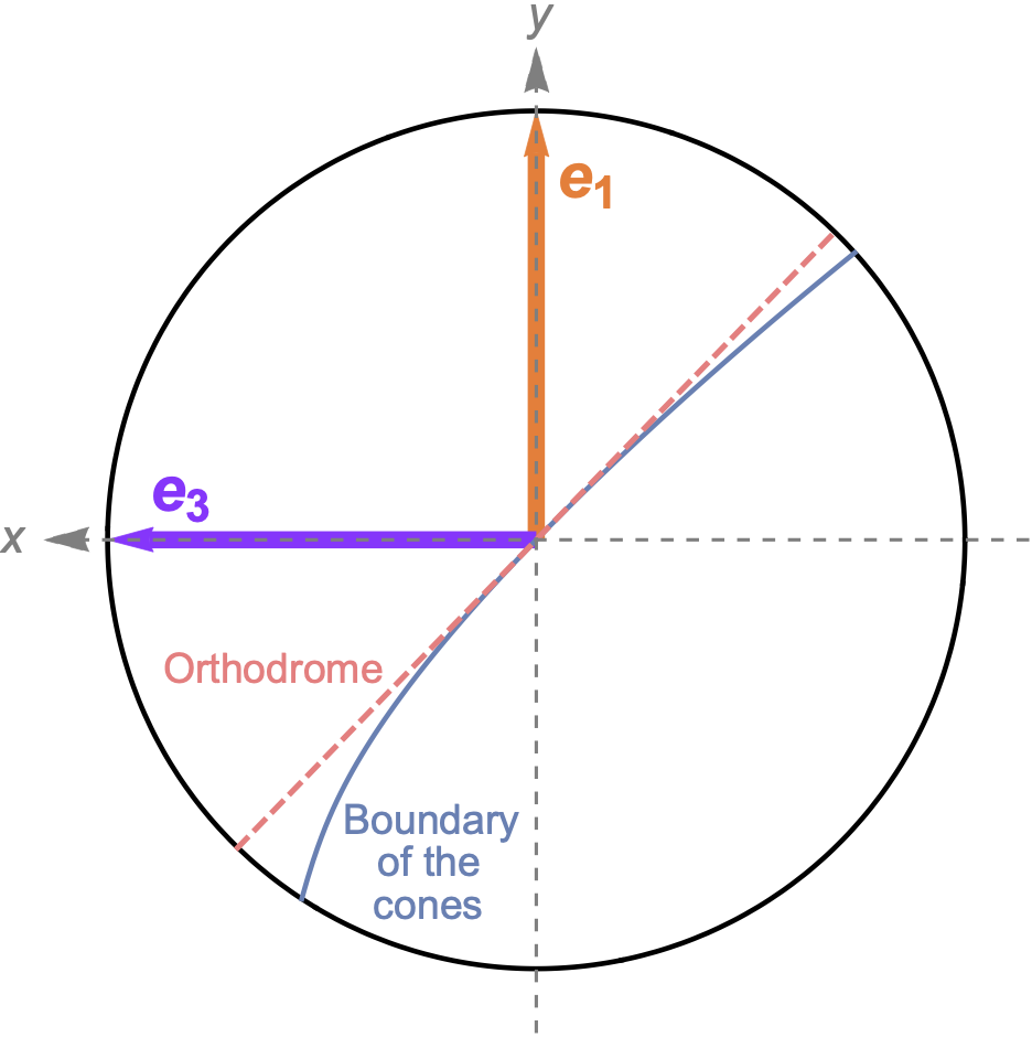
Figure 9: The boundary of the escape and capture cones projected onto the plane spanned by $\mathbf{e}_{3}$ and $\mathbf{e}_{1}$ for $r/M=r_{s}^{(0)}/M\approx 2.431$ in the equatorial plane of a Kerr spacetime with $a_{*}=0.99$. The projected orthodrome that is tangent to the boundary at $(\xi,\eta)=(\pi/2,\pm\pi/2)$ is shown by the dashed line. Because the boundary of the cones is convex upward, the orthodrome is included in the escape cone except at $(\xi,\eta)=(\pi/2,\pm\pi/2)$.

Figure 9 shows an example of the projected boundary of the escape and capture cones and the projected orthodrome that is tangent to the boundary at $(\xi,\eta)=(\pi/2,\pm\pi/2)$ on the two-dimensional plane spanned by $\mathbf{e}_{3}$ and $\mathbf{e}_{1}$ for $r=r_{s}^{(0)}$ on the equatorial plane in the case $a_{*}=0.99$. The projected boundary of the cones becomes a curve that passes through the origin, and the projected orthodrome becomes a tangent line to the curve of the projected boundary at the origin. The projected orthodrome divides the unit disk into the upper and lower half-disks, and then, the condition that the orthodrome is included in the escape cone except for $(\xi,\eta)=(\pi/2,\pm\pi/2)$ is equivalent to that the projected boundary of the cones is included in the lower half-disk. This is guaranteed by the fact that the projected boundary is convex upward, as indicated by the inequality of Eq. (60). Therefore, we can safely declare that $r=r_{s}^{(0)}$ is the ODH.

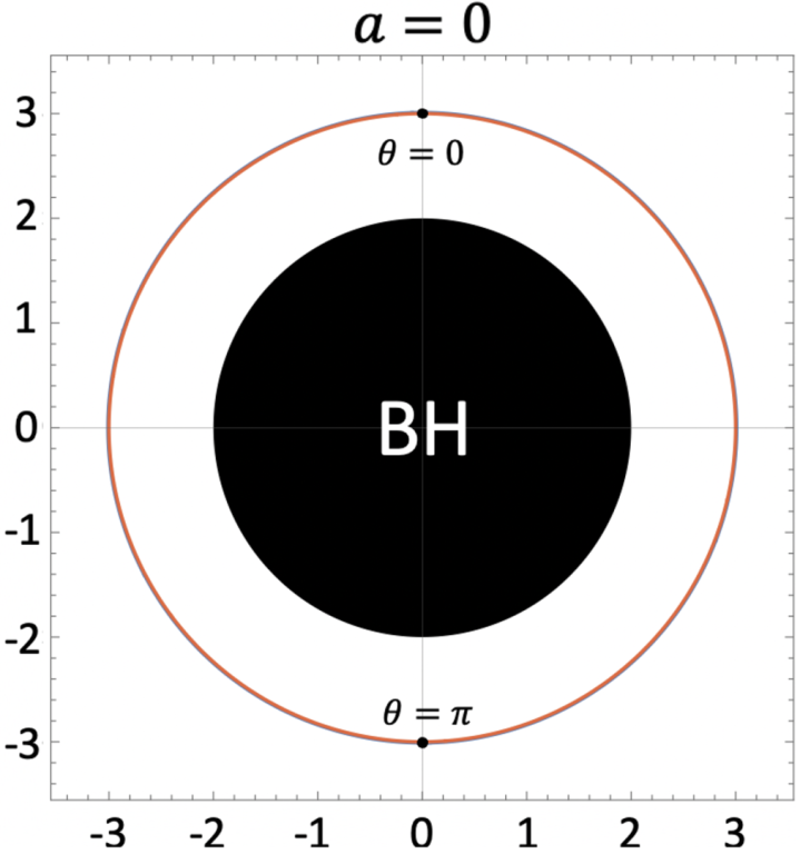
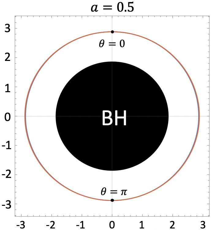
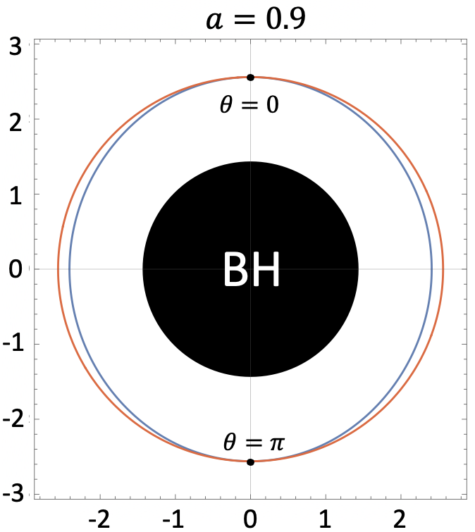
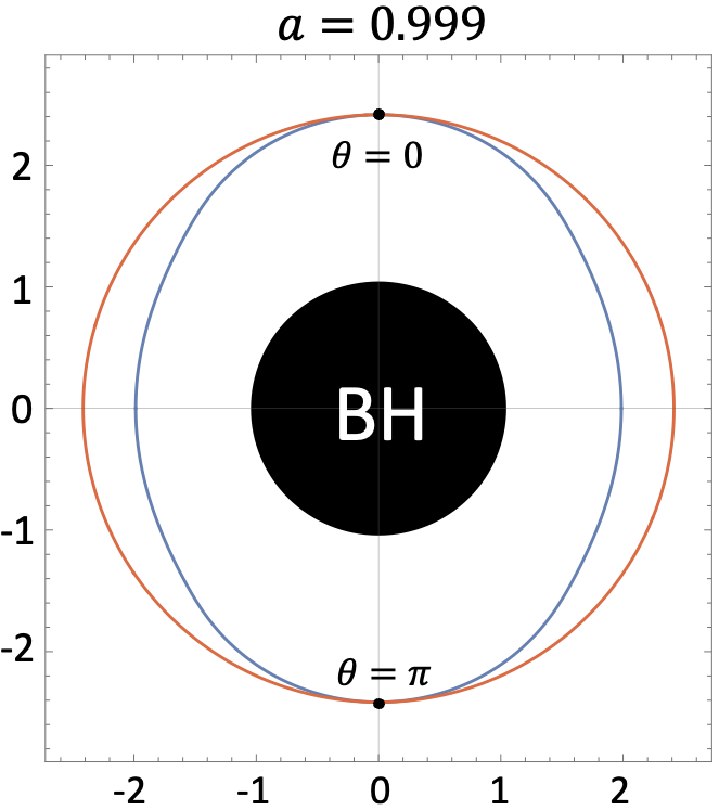
Figure 10: The outer dark horizons (orange) and inner dark horizons (blue) in the Kerr spacetime seen from a distant position on the equatorial plane for $a_{*}=0,0.5,0.9,0.999$. The unit of both axes is $M$. The central black disks represent black holes (BHs). In the case of $a_{*}=0$, the outer dark horizon and the inner dark horizon coincide with each other due to Thm. 3.19.

We depicted the ODH in the Kerr spacetime, i.e., $r=r_{s}^{(0)}$ in Fig. 10 for the cases $a_{*}=0.0$, $0.5$, $0.9$, and $0.999$. In Fig. 10, the IDHs, which will be discussed in the next subsection, are shown by blue closed curves.

6.4 Inner Dark Horizon in Kerr spacetime

We now focus our attention to the IDH. The IDH requires numerical calculations to specify its location. As the numerical strategy, we make use of Thm. 3.8 and Prop. 3.10, and in this case, the positions of the boundary of the escape and capture cones at $\eta=0$ and $\pi$ play an important role. Suppose that the position of the boundary is given by $\xi=\xi_{+}$ at $\eta=0$ (i.e., $\cos\eta=+1$), and $\xi=\xi_{-}$ at $\eta=\pi$ (i.e., $\cos\eta=-1$). Then, $\xi_{+}\leq\xi\leq\pi$ at $\eta=0$ and $\xi_{-}\leq\xi\leq\pi$ at $\eta=\pi$ belong to the capture cone, while $0\leq\xi<\xi_{+}$ at $\eta=0$ and $0\leq\xi<\xi_{-}$ at $\eta=\pi$ belong to the escape cone. For a spacetime point $p$ that satisfies $\xi_{-}+\xi_{+}>\pi$, a pair of antipodal points exists in the escape cone, such as $(\xi,\eta)=((\xi_{+}-\xi_{-}+\pi)/2,0)$ and $((\xi_{-}-\xi_{+}+\pi)/2,\pi)$. Then, the point $p$ is not in the IDD from Thm. 3.8.

At the distant place $r\gg M$, the value of $\xi_{+}+\xi_{-}$ is close to $2\pi$. As $r$ is decreased, the value of $\xi_{+}+\xi_{-}$ becomes smaller. Suppose that a point $p$ satisfying $\xi_{+}+\xi_{-}=\pi$ is found. At that point, we can introduce the orthodrome that is tangent to the boundary of the escape cone at $(\xi,\eta)=(\xi_{+},0)$ and $(\xi_{-},\pi)$ since these two points are antipodal to each other and the tangent vectors of the boundary of cones at these two points both have vanishing $\xi$ components due to the symmetries in the transformation $\eta\to-\eta$ and in the transformation $\eta-\pi\to-(\eta-\pi)$. If that orthodrome is included in the capture cone, the point $p$ is on the IDH due to Prop. 3.10. Therefore, our strategy is firstly to solve for the point where $\xi_{+}+\xi_{-}=\pi$, and secondly to confirm that the obtained point is actually the point of the IDH.

Let us start from solving for a position that satisfies $\xi_{+}+\xi_{-}=\pi$. We focus on each $\theta$-constant surface in the Kerr spacetime. For each $r$, the formulas to parametrically specify the boundary of the escape cone are given by Eqs. (53a) and (53b) with Eqs. (56) and (57). These formulas are symbolically written as $\sin\xi=\sin\xi(r,r_{\rm s})$ and $\cos\eta=\cos\eta(r,r_{\rm s})$. Writing the values of $r_{s}$ that satisfy $\eta=0$ and $\pi$ (i.e., $\cos\eta=\pm 1$) as $r_{\rm s}^{\pm}$, we have $\pm 1=\cos\eta(r,r_{\rm s}^{\pm})$. Then, $\xi_{\pm}$ are determined by $\sin\xi_{\pm}=\sin\xi(r,r_{\rm s}^{\pm})$. Since $\xi_{+}+\xi_{-}=\pi$ leads to the condition $\sin\xi_{+}\ =\ \sin\xi_{-}$, we obtain the set of equations to determine the radius $r_{\rm IDH}$ of the IDH for a given $\theta$:

$$\sin\xi(r_{\rm IDH},r_{\rm s}^{+})\ =\ \sin\xi(r_{\rm IDH},r_{\rm s}^{-}),$$ (63a)

$$+1 = \cos\eta(r_{\rm IDH},r_{\rm s}^{+}),$$ (63b)

$$-1 = \cos\eta(r_{\rm IDH},r_{\rm s}^{-}).$$ (63c)

This set of equations can be solved numerically easily. Except for $\theta=0$ and $\pi$, the value of $r_{\rm IDH}$ is smaller than $r_{s}^{(0)}$ (interested readers can see blue curves of Fig. 10 in advance).

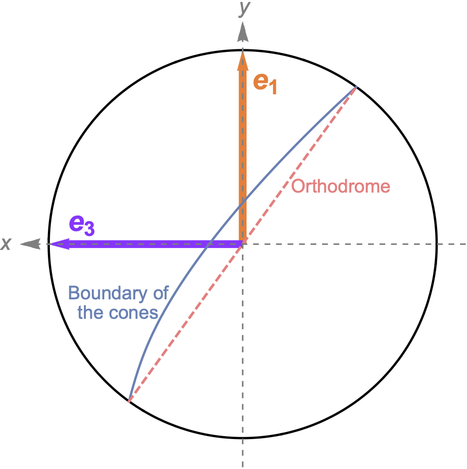
Figure 11: The boundary of the escape and capture cones projected onto the plane spanned by $\mathbf{e}_{3}$ and $\mathbf{e}_{1}$ for $r/M=r_{\rm IDH}/M\approx 2.092$ in the equatorial plane of a Kerr spacetime with $a_{*}=0.99$. The orthodrome tangent to the boundary of the cones at $(\xi,\eta)=(\xi_{+},0)$ and $(\xi_{-},\pi)$ is shown by the dashed line. Because the boundary of the cones is convex upward, the orthodrome is included in the capture cone.

Let us move on to the next step at which we check the obtained surface, $r=r_{\rm IDH}(\theta)$, is actually the IDH. Figure 11 shows an example of the boundary of the escape and capture cones and the orthodrome tangent to it that are projected onto the two-dimensional plane spanned by $\mathbf{e}_{3}$ and $\mathbf{e}_{1}$ for $r=r_{\rm IDH}$ on the equatorial plane in the case of $a_{*}=0.99$. On the two-dimensional plane, the curve of the projected boundary and the line of the projected orthodrome have the same endpoints on the unit circle. By the projected orthodrome, the projected two-sphere of emission directions is divided into the upper and lower half-disks, and the condition that the orthodrome is included in the capture cone is equivalent to that the projected boundary of the cones is included in the upper half-disk. This is guaranteed by the fact that the curve of the projected boundary of the cones is convex upward, as indicated by the inequality of Eq. (60). Therefore, the obtained numerical solution $r=r_{\rm IDH}(\theta)$ is confirmed to be the IDH.

In Fig. 10, we plot the IDH with blue closed curves in the Kerr spacetime with several Kerr parameters. The ODH and IDH both exist in the Kerr spacetime due to Props. 3.14 and 3.18. In the case of $a_{*}=0$, the ODH and IDH coincide with each other by Thm. 3.19, and their radii are given by $3M$. In the case of $a_{*}>0$, the IDH coincides with the ODH only on the rotation axis, and at other positions, the ODH is located in the outside region of the IDH due to Cor. 3.9. In each case, the ODH is given by $r=r_{s}^{(0)}$, which coincides with the edge of the shadow observed from infinity on the axis.

7 Conclusion & Discussion

In this paper, we have proposed new concepts dark horizons (the outer dark horizon, ODH for short, and the inner dark horizon, IDH for short) as generalizations of the photon sphere, from static and spherically symmetric spacetimes to general asymptotically flat spacetimes. In short, the dark horizons are defined with some timelike vector field $T^{\mu}$ or the timeslice $\Sigma_{t}$ which can be chosen depending on the physical context, and the dark horizons are defined as the boundary of the region where escape (capture) cone is large (small) enough in the frame associated with $T^{\mu}$ or $\Sigma_{t}$. We have focused on four-dimensional asymptotically flat spacetimes. We can also apply the same definitions in higher dimensions as the dark horizons. In higher-dimensional case, the positive condition for $\Omega_{i}$, which is defined in Eq. (15), is not needed in Lems. 3.13, 3.17, Props. 3.14, 3.18.

We have strictly shown several statements for the dark horizons. First, the ODD and IDD are both absent in the Minkowski spacetime (see Props. 3.11 and 3.15) and are both present in the spacetime with black hole(s) under a natural assumption (see Thms. 3.12 and 3.16). Second, two dark horizons both exist in black hole spacetime under a natural condition (see Props. 3.14 and 3.18). Third, the IDH is typically located inside of or coinsides with the ODH (see Cor. 3.9). Fourth, in spherical symmetric spacetimes, the ODH and IDH coincide with each other. In addition, we have clarified explicit shapes of the dark horizons in the Vaidya and Kerr spacetimes.

In order to study the relation between the dark horizons and the photon sphere, we defined the visible photon sphere in static and spherically symmetric spacetimes as an unstable photon sphere from which perturbed photons around the photon sphere can move away and reach future null infinity. Then, we have shown, in Thm. 4.5, that any visible photon sphere is a dark horizon and that the outermost photon sphere is the outermost dark horizon in Thm. 4.5. Indeed, the visible photon sphere captures the essential properties of the photon sphere— the properties such that it represents the boundary of the observable region, satisfies the areal inequality Eq. (1) for the outermost visible photon sphere, and serves as an indicator for a strong gravity region.

The dark horizons are defined by referring to null geodesics reaching future null infinity, at which ideal observers are supposed to be distributed. In this sense, the locations of dark horizons are affected by the geometry not only on dark horizons but also the one far away from dark horizons. This distinguishes the concepts of the dark horizon from some of other generalizations of the photon sphere defined in terms of the local geometrical quantities, such as the extrinsic curvature (e.g. Shiromizu:2017ego ; Yoshino:2019dty ).

The dark horizons rather resemble the concept of the black room of Ref. Siino:2021kep in the sense that these are defined in terms of the global behavior of the null geodesics. Here, the black room is defined as a spacetime region such that any photon entering the black room never goes out to the outside region of it. According to this definition, photons emitted at a point on the boundary of the black room in the tangential directions to the boundary must either propagate on the boundary of the black room or fall into the black room. Then, if we prepare a timelike vector field $T^{\mu}$ which is tangent to the boundary of the maximal black room, the IDD associated with it must include the boundary of the black room.

The main difference between the black room and the dark horizons is as follows. On the one hand, the condition for a specific point to be in the black room refers to the global behavior of the null geodesics both in the future and past directions of this point, and therefore, it cannot have past endpoints. Then, the black room does not exist in spacetimes in which a black hole exists only after the gravitational collapse. In addition, the black room does not exist for spacetimes without a black hole Siino:2021kep . On the other hand, each point of the dark horizons refers to the global behavior of null geodesics only in the future side of this point. As a result, it is possible for dark horizons to exist in black hole spacetimes with the gravitational collapse. In addition, it is also possible that the dark horizons exist in spacetimes without a black hole and they coincide with the visible photon sphere. These differences would originate from the difference of the supposed positions of the light sources in these concepts. The black room concept would correspond to the situation where light sources are located at past null infinity (as the simple theoretical models of the black hole shadows), whereas the dark horizons correspond to the situation where light sources are located in and around the ODH and IDH, which are typically near the black hole. We expect that the dark horizons serve as important concepts to describe the properties of the shadows whose light sources distribute in strong gravity regions in varieties of asymptotically flat spacetimes.

Appendix A Detailed Proof of Lem. 4.4

In Sec. 4, we presented Lem. 4.4 based on an intuitive, but physical argument. In this appendix, we provide a more rigorous proof of Lem. 4.4 as follows.

As a preparation, let us show that for all spacelike vectors $n_{2}^{\mu}$ orthogonal to $T^{\mu}:=(\partial_{t})^{\mu}/\sqrt{f(r)}$, there exists a null vector $k^{\mu}$ which is an orthogonal vector to both $n_{2}^{\mu}$ and $(dr)^{\mu}$. The null vector $k^{\mu}$ can be constructed as follows. Equation (25) gives us $g_{\mu\nu}\left(dr\right)^{\mu}\left(dt\right)^{\nu}=g^{rt}=0$. This means that $(dr)^{\mu}$ is orthogonal to $T^{\mu}$. Since we consider a four-dimensional manifold, we can take a vector $n_{3}^{\mu}$ orthogonal to all of $T^{\mu}$, $n_{2}^{\mu}$, and $(dr)^{\mu}$. We can construct a null vector $k^{\mu}$ as a linear combination of $n_{3}^{\mu}$ and $T^{\mu}$. Then, the null vector $k^{\mu}$ is orthogonal to both $n_{2}^{\mu}$ and $(dr)^{\mu}$, which completes the preparation.

Let a point $P_{0}(t_{0},r_{0},\theta_{0},\phi_{0})$ be in the dark domain. By the definition of the IDD, there exists a spacelike vector $n^{\mu}$ orthogonal to $T^{\mu}$, such that for all null geodesics which are orthogonal to $n^{\mu}$ at $P_{0}$ do not reach future null infinity. Therefore, we see that there exists a null geodesic whose tangent vector is orthogonal to both $n^{\mu}$ and $(dr)^{\mu}$ at $P_{0}$ and does not reach future null infinity. By the orthogonality to $(dr)^{\mu}$, we have $r^{\prime}=0$ at this point. Thus, by Eq. (29) and the equivalence between $b=B(r)$ and $R=0$, the point $P_{0}$ corresponds to a point on $b=B(r)$ on $r-b$ plane. In the case of $dB/dr(r_{0})>0$, from Eq. (32), it is easy to see that $dR/dr>0$ holds outside the horizon, which gives us $r^{\prime\prime}>0$ from Eq. (33). Thus, we have $r^{\prime}>0$ right after $P_{0}$. The sign of $r^{\prime}$ will be flipped, or $r$ asymptotes to some constant because the null geodesic will not reach future null infinity. If the sign of $r^{\prime}$ will be flipped, $r^{\prime}$ will experience $r^{\prime}=0$, which means that there exists $\tilde{r}_{0}>r_{0}$ such that $B(r_{0})=B(\tilde{r}_{0})$. If $r$ asymptotes to some constant $r_{c}$, that is,

$$\lim_{r\to r_{c}}r^{\prime}=0$$

holds, then from Eq. (29), we have

$$\lim_{r\to r_{c}}B(r)=b,$$

which gives us $b=B(r_{c})$. Thus, we see that there exists $\tilde{r}_{0}>r_{0}$ such that $B(r_{0})=B(\tilde{r}_{0})$ (see Fig. 4). In the case of $dB/dr(r_{0})<0$, there exists $\tilde{r}_{0}>r_{0}$ such that $B(r_{0})=B(\tilde{r}_{0})$ because $B(r)$ is a continuous function of $r$ and we have

$$\lim_{r\to\infty}B(r)=\infty$$

by the fall-off condition. Therefore, in either case, there exists $\tilde{r}_{0}>r_{0}$ such that $B(r_{0})=B(\tilde{r}_{0})$. Combining with the case with $dB/dr(r_{0})=0$, we see that $dB/dr(r_{0})=0$ holds or there exists $\tilde{r}_{0}>r_{0}$ such that $B(r_{0})=B(\tilde{r}_{0})$.

Conversely, consider any point $P_{0}$ at which $dB/dr(r_{0})=0$ holds or there exists $\tilde{r}_{0}>r_{0}$ such that $B(r_{0})=B(\tilde{r}_{0})$. We will discuss null geodesics which are orthogonal to $(dr)^{\mu}$ at $P_{0}$. When $dB/dr(r_{0})=0$ holds, Eq. (33) gives us $r^{\prime\prime}=0$ when $r^{\prime}=0$. Thus, all null geodesics which are orthogonal to $(dr)^{\mu}$ at $P_{0}$ stay on $r=r_{0}$ hypersurface and do not reach future null infinity. Let us consider the other situation, in which there exists $\tilde{r}_{0}>r_{0}$ such that $B(r_{0})=B(\tilde{r}_{0})$. We define $\tilde{r}_{0{\rm m}}$ as the minimum of such $\tilde{r}_{0}$. We classify the situation into three cases based on the sign of $dB/dr(\tilde{r}_{0{\rm m}})$. In the case of $dB/dr(\tilde{r}_{0{\rm m}})\neq 0$, for sufficiently small $\epsilon>0$, either $b>B(\tilde{r}_{0{\rm m}}-\epsilon)$ or $b>B(\tilde{r}_{0{\rm m}}+\epsilon)$ holds. Since $b>B(r)$ is the forbidden region and $b=B(\tilde{r}_{0{\rm m}})$, the null geodesic will not reach future null infinity. In the case of $dB/dr(\tilde{r}_{0{\rm m}})=0$, we can show as follows that the null geodesic does not reach $r=\tilde{r}_{0{\rm m}}$. Suppose, for the sake of contradiction, that the null geodesic reaches $r=\tilde{r}_{0{\rm m}}$. Here, we have $r^{\prime}=0$ and $r^{\prime\prime}=0$ at this point. Thus, the null geodesic must be on $r=\tilde{r}_{0{\rm m}}$ in the past. This contradicts to $r=r_{0}<\tilde{r}_{0{\rm m}}$ in the past. Therefore, the null geodesic does not reach $r=\tilde{r}_{0{\rm m}}(>r_{0})$. Thus, in any case, all null geodesics which are orthogonal to $(dr)^{\mu}$ at $P_{0}$ do not reach future null infinity. Thus, the point $P_{0}$ is in the dark domain.

Therefore, a point $P_{0}$ is in the dark domain if and only if $dB/dr(r_{0})=0$ or there exists $\tilde{r}_{0}>r_{0}$ such that $B(r_{0})=B(\tilde{r}_{0})$.

Appendix B Proof of the inequalities of Eqs. (59) and (60)

In this appendix, we present the proof of the inequalities of Eqs. (59) and (60) in the analysis of the Kerr spacetime of Sec. 6. Before starting, it is useful to discuss the range of values that $r_{s}$ can take in Eqs. (56) and (57). Since the range of $r_{s}$ depends on $\theta$, we regard that the range is given by $r_{\rm SPO}^{(+)}(\theta)\leq r_{s}\leq r_{\rm SPO}^{(-)}(\theta)$ for a given $\theta$, where $r=r_{\rm SPO}^{(+)}(\theta)$ and $r=r_{\rm SPO}^{(-)}(\theta)$ correspond to the prograde and retrograde spherical photon orbits, respectively. In the equatorial plane, they take the values (e.g. Frolov:1998 )

$$r_{\rm SPO}^{(\pm)}(\pi/2)=2M\left\{1+\cos\left[\frac{2}{3}\arccos\left(\mp a_{*}\right)\right]\right\}.$$ (64)

As the value of $\theta$ is decreased, the values of $r_{\rm SPO}^{(+)}(\theta)$ increases, while the value of $r_{\rm SPO}^{(-)}(\theta)$ decreases, and both converge to $r_{s}^{(0)}$ of Eq. (62) in the limit $\theta\to 0$. In any case, it is sufficient to know that the value of $r_{s}$ satisfies $r_{s}>r_{\rm H}^{+}>M$, where $r_{\rm H}^{+}$ is defined in Eq. (41), since the spherical photon orbits are located outside the event horizon.

As a preparation, we show that the inequality

$$A-2Mabr>0$$ (65)

holds on the boundary of the escape and capture cones, where $A$ is given in Eq. (40). Since the value of $b$ is parametrically given by Eq. (56) on the boundary of the cones, after some algebra, we have

$$A-2Mabr\,=\,2Mr\Delta(r_{s})+(r^{2}+2Mr+a^{2}\cos^{2}\theta)\Delta(r)\\ +\frac{2M^{2}r\left[(r-r_{\rm H}^{-})(r_{s}-r_{\rm H}^{+})+(r-r_{\rm H}^{+})(r_{s}-r_{\rm H}^{-})\right]}{r_{s}-M},$$ (66)

where $\Delta(r)$ is the same as $\Delta$ given in Eq. (40), $\Delta(r_{s})$ is the same as $\Delta(r)$ but $r$ being replaced by $r_{s}$, and the definitions of $r_{\rm H}^{\pm}$ are given in Eq. (41). The right-hand side of this equation is manifestly positive for $r>r_{\rm H}^{+}$ and $r_{s}>r_{\rm H}^{+}$, and therefore, the inequality of Eq. (65) is satisfied. This inequality means that on the boundary of the cones, we do not have to take an absolute value in the denominator of Eq. (53a), and $\mathrm{sgn}(A-2Mabr)$ in Eq. (53b) can be omitted.

We now present the proof of the inequalities of Eqs. (59) and (60). In the main article, we introduced the coordinates $(\xi,\eta)$ on the two-sphere of emission directions through Eq. (46), and in the paragraph with Eq. (59), we introduced the Cartesian coordinates $(x,y)$ on the unit disk that is the two-sphere projected onto the plane spanned by $\mathbf{e}_{3}$ and $\mathbf{e}_{1}$. The relation between these two coordinate systems is

$$x = \sin\xi\cos\eta,$$ (67a)

$$y = \cos\xi.$$ (67b)

Through Eqs. (53a), (53b), (56), and (57), the projected boundary of the escape and capture cones is given in the form $x=x(r_{s})$ and $y=y(r_{s})$. More specifically,

$$x = \frac{b\Sigma\sqrt{\Delta}}{(A-2Mabr)\sin\theta},$$ (68a)

$$y = \frac{(r_{s}-r)\sqrt{H(r_{s})A}}{(r_{s}-M)(A-2Mabr)},$$ (68b)

with

$$H(r_{s})\,=\,(r_{s}-M)^{2}\left[(r_{s}+r-2M)^{2}+4M(r-M)\right]+4M(M^{2}-a^{2})r_{s}.$$ (69)

Equation (68b) with Eq. (69) gives the explicit form of the right-hand side of Eq. (58), i.e., the analytic expression of $\cos\xi$ for the correct boundary of the cones.

The quantity $dy/dx$ is calculated as

$$\frac{dy}{dx}\ =\ \frac{y^{\prime}}{x^{\prime}}\ =\ -\frac{a\sin\theta}{\Sigma}\sqrt{\frac{\Delta}{AH(r_{s})}}\left[rg(r_{s})+a^{2}\cos^{2}\theta h(r_{s})\right],$$ (70)

where the prime denotes the derivative with respect to $r_{s}$ in this appendix, and

$$g(r_{s}) = (r+M)r_{s}(r_{s}+r)+M(3r_{s}^{2}+r^{2}),$$ (71)

$$h(r_{s}) = (r_{s}-M)^{2}+(r-M)(r_{s}+M).$$ (72)

Because $g(r_{s})$ and $h(r_{s})$ are obviously positive for $r_{s}>M$ and $r>M$, the right-hand side of Eq. (70) is nonpositive for $a>0$, and becomes zero on and only on the rotation axis at which $\sin\theta=0$ is satisfied . Therefore, the inequality of Eq. (59) has been proved.

The quantity $d^{2}y/dx^{2}$ is calculated as

$$\frac{d^{2}y}{dx^{2}}\ =\ -\frac{Ma^{2}\sin^{2}\theta(r+3r_{s})(r_{s}-M)^{3}(A-2Mabr)^{3}}{\Sigma^{2}A^{3/2}K(r_{s})H(r_{s})^{3/2}},$$ (73)

where

$$K(r_{s})\ =\ (r_{s}-M)^{3}+M(M^{2}-a^{2}).$$ (74)

Then, the right-hand side of Eq. (73) is nonpositive for the black hole configuration $M^{2}>a^{2}$ since $r_{s}>M$, $r>M$, and the inequality of Eq. (65) hold, and becomes zero on and only on the rotation axis. Therefore, the inequality of Eq. (60) has been proved.

References

- (1) K. Akiyama et al. (Event Horizon Telescope Collaboration), “First M87 Event Horizon Telescope results. I. The shadow of the supermassive black hole,” Astrophys. J. Lett. 875, L1 (2019).
- (2) K. Akiyama et al. [Event Horizon Telescope], “First Sagittarius A* Event Horizon Telescope Results. I. The Shadow of the Supermassive Black Hole in the Center of the Milky Way,” Astrophys. J. Lett. 930, no.2, L12 (2022).
- (3) K. Akiyama et al. [Event Horizon Telescope], “First M87 Event Horizon Telescope Results. V. Physical Origin of the Asymmetric Ring,” Astrophys. J. Lett. 875, no.1, L5 (2019).
- (4) H. M. Wang, Y. M. Xu and S. W. Wei, “Shadows of Kerr-like black holes in a modified gravity theory,” JCAP 03, 046 (2019).
- (5) J. W. Moffat and V. T. Toth, “Masses and shadows of the black holes Sagittarius A* and M87* in modified gravity,” Phys. Rev. D 101, no.2, 024014 (2020).
- (6) M. Khodadi and E. N. Saridakis, “Einstein-Æther gravity in the light of event horizon telescope observations of M87*,” Phys. Dark Univ. 32, 100835 (2021).
- (7) C. M. Claudel, K. S. Virbhadra, and G. F. R. Ellis, “The Geometry of photon surfaces,” J. Math. Phys. 42, 818 (2001).
- (8) K. S. Virbhadra and G. F. R. Ellis, “Schwarzschild black hole lensing,” Phys. Rev. D 62, 084003 (2000).
- (9) R. Q. Yang and H. Lu, “Universal bounds on the size of a black hole,” Eur. Phys. J. C 80 no.10, 949 (2020).
- (10) H. Lu and H. D. Lyu, “Schwarzschild black holes have the largest size,” Phys. Rev. D 101 no.4, 044059 (2020).
- (11) T. Shiromizu, Y. Tomikawa, K. Izumi and H. Yoshino, “Area bound for a surface in a strong gravity region,” PTEP 2017, no.3, 033E01 (2017).
- (12) H. Yoshino, K. Izumi, T. Shiromizu and Y. Tomikawa, “Extension of photon surfaces and their area: Static and stationary spacetimes,” PTEP 2017, no.6, 063E01 (2017).
- (13) L. M. Cao and Y. Song, “Quasi-local photon surfaces in general spherically symmetric spacetimes,” Eur. Phys. J. C 81, 714 (2021).
- (14) H. Yoshino, K. Izumi, T. Shiromizu and Y. Tomikawa, “Transversely trapping surfaces: Dynamical version,” PTEP 2020, no.2, 023E02 (2020).
- (15) M. Siino, “Causal concept for black hole shadows,” Class. Quant. Grav. 38, no.2, 025005 (2021).
- (16) M. Siino, “Black hole shadow and wandering null geodesics,” Phys. Rev. D 106, no.4, 044020 (2022).
- (17) H. Bondi, M. G. J. van der Burg and A. W. K. Metzner, “Gravitational waves in general relativity. VII. Waves from axisymmetric isolated systems,” Proc. Roy. Soc. Lond. A 269, 21-52 (1962).
- (18) R. K. Sachs, “Gravitational waves in general relativity. VIII. Waves in asymptotically flat space-times,” Proc. Roy. Soc. Lond. A 270, 103-126 (1962).
- (19) K. Tanabe, S. Kinoshita and T. Shiromizu, “Asymptotic flatness at null infinity in arbitrary dimensions,” Phys. Rev. D 84, 044055 (2011).
- (20) S. Hollands and A. Ishibashi, “Asymptotic flatness at null infinity in higher dimensional gravity,” arXiv:hep-th/0311178.
- (21) S. Hollands and A. Ishibashi, “Asymptotic flatness and Bondi energy in higher dimensional gravity,” J. Math. Phys. 46, 022503 (2005).
- (22) A. Ishibashi, “Higher Dimensional Bondi Energy with a Globally Specified Background Structure,” Classical Quantum Gravity 25, 165004 (2008).
- (23) M. Amo, K. Izumi, Y. Tomikawa, H. Yoshino and T. Shiromizu, “Asymptotic behavior of null geodesics near future null infinity: Significance of gravitational waves,” Phys. Rev. D 104 (2021) no.6, 064025 [erratum: Phys. Rev. D 107, 029901 (2023)].
- (24) M. Amo, T. Shiromizu, K. Izumi, H. Yoshino and Y. Tomikawa, “Asymptotic behavior of null geodesics near future null infinity. II. Curvatures, photon surface, and dynamically transversely trapping surface,” Phys. Rev. D 105, no.6, 064074 (2022).
- (25) M. Amo, K. Izumi, Y. Tomikawa, H. Yoshino and T. Shiromizu, “Asymptotic behavior of null geodesics near future null infinity. III. Photons towards inward directions,” Phys. Rev. D 106, no.8, 084007 (2022) [erratum: Phys. Rev. D 107, 029902 (2023)].
- (26) M. Amo, K. Izumi, Y. Tomikawa, T. Shiromizu and H. Yoshino, “Asymptotic behavior of null geodesics near future null infinity IV: Null-access theorem for generic asymptotically flat spacetime,” [arXiv:2305.01767 [gr-qc]].
- (27) W. Israel, “Singular hypersurfaces and thin shells in general relativity,” Nuovo Cim. B 44S10, 1 (1966) [erratum: Nuovo Cim. B 48, 463 (1967)].
- (28) K. Ogasawara and T. Igata, “Complete classification of photon escape in the Kerr black hole spacetime,” Phys. Rev. D 103 (2021) no.4, 044029.
- (29) B. Carter, “Global structure of the Kerr family of gravitational fields,” Phys. Rev. 174 (1968), 1559-1571.
- (30) M. Walker and R. Penrose, “On quadratic first integrals of the geodesic equations for type [22] spacetimes,” Commun. Math. Phys. 18, 265-274 (1970).
- (31) Y. Koga, N. Asaka, M. Kimura and K. Okabayashi, “Dynamical photon sphere and time evolving shadow around black holes with temporal accretion,” Phys. Rev. D 105, no.10, 104040 (2022).
- (32) V. P. Frolov and I. D. Novikov, Black Hole Physics: Basic Concepts and New Developments, (Kluwer Academic Publishers, Dordrecht and Boston, 1998).
- (33) E. Teo, “Spherical orbits around a Kerr black hole,” Gen. Rel. Grav. 35, 1909, (2003).