Imprints of phase transitions on Kasner singularities

Abstract

Under the AdS/CFT correspondence, asymptotically AdS geometries with backreaction can be viewed as CFT states subject to a renormalization group (RG) flow from an ultraviolet (UV) description towards an infrared (IR) sector. For black holes however, the IR point is the horizon, so one way to interpret the interior is as an analytic continuation to a “trans-IR” imaginary-energy regime. In this paper, we demonstrate that this analytic continuation preserves some imprints of the UV physics, particularly near its “endpoint” at the classical singularity. We focus on holographic phase transitions of geometric objects in round black holes. We first assert the consistency of interpreting such black holes, including their interiors, as RG flows by constructing a monotonic $a$-function. We then explore how UV phase transitions of entanglement entropy and scalar two-point functions, each of which are encoded by bulk geometry under the holographic mapping, are connected to the structure of the near-singularity geometry, which is characterized by Kasner exponents. Using 2d holographic flows triggered by relevant scalar deformations as test beds, we find that the 3d bulk’s near-singularity Kasner exponents can be viewed as functions of the UV physics precisely when the deformation is nonzero.

1 Introduction

A renormalization group (RG) flow is a contour in the space of QFT couplings that describes the coarse graining of a high-energy (UV-complete) theory to a low-energy (IR) description Wilson:1973jj; Polchinski:1983gv. We integrate out all high-energy modes above some cutoff energy to get an effective QFT. The flow itself consists of all such effective theories and is thus parameterized by the cutoff. Furthermore, both the IR and UV theories are conformal-invariant fixed points of the flow and so are conformal field theories (CFTs). Most importantly, the IR theory may have imprints of the UV physics as remnants of the integration procedure, even though the IR is mostly insensitive to the UV.

A guiding principle of modern quantum gravity research is the AdS/CFT correspondence Maldacena:1997re equating weakly coupled “bulk” gravity on $(d+1)$-dimensional anti-de Sitter (AdS) space to strongly coupled CFT physics on the $d$-dimensional boundary of AdS. AdS/CFT describes a “holographic” class of RG flows Balasubramanian:1999jd. The energy cutoff is associated with the radial extra dimension of the bulk theory, with the UV fixed point being the boundary CFT, so this RG flow essentially describes the emergence of holographic bulk spacetime. The flow dynamics are encoded by the gravitational theory deBoer:1999tgo; deBoer:2000cz; Bianchi:2001kw; Fukuma:2002sb; Papadimitriou:2004ap; Papadimitriou:2005ii, which must include a bulk matter sector dual to some relevant deformation of the UV theory. As the bulk theory is weakly coupled, it is a tractable setting in which one can study imprints of UV physics in the IR sector.

Gravitational theories typically feature black holes, and these are dual to states of a canonical ensemble at fixed temperature. For example, large AdS black holes are dual to thermal CFT states Witten:1998zw; Hubeny:2014bla; hartmanhepQG. From the perspective of holographic RG flow, such a black hole with matter-induced backreaction describes an RG flow from a UV thermal state towards an IR fixed point associated with the horizon. However, the classical geometry does not stop at the horizon; there is also an interior region in which the radial dimension is timelike, rather than spacelike. Nonetheless, we may insist that the black-hole interior is also part of an RG flow. We would then claim that the interior corresponds to a “trans-IR” part of the flow Frenkel:2020ysx; Caceres:2022smh defined as an analytic continuation of the exterior RG flow to imaginary energies. It is further natural to infer that the UV physics leaves an imprint on the trans-IR regime. Exploring such imprints is the goal of this paper.

We emphasize that the trans-IR picture is a working interpretation rather than a firm, established statement. In particular, it is not clear what the actual “points” along this interior RG flow (reached by integrating out all real-energy modes and integrating in “imaginary-energy” modes) would represent in field-theoretic terms, although some progress has been made by Hartnoll:2022snh. While we do not directly tackle this issue in this paper, the study herein is meant to provide some internal consistency to the trans-IR perspective of the black-hole interior as a coarse-graining flow. To this end, we first build on previous work Caceres:2022smh; Caceres:2022hei exploring the existence of monotonic “degree-of-freedom-counting” functions.

Furthermore, we explore how phase transitions in the UV are encoded by the trans-IR part of the flow. We focus on the following two holographic phase transitions in black holes with spherical horizons:

• the deviation of a boundary subregion’s entanglement from the Araki–Leib bound Araki:1970ba described by the holographic entanglement plateaux of Hubeny:2013gta; and

• the connected/disconnected phase transition of a thermal two-point function of a heavy scalar operator $\mathcal{O}_{\text{H}}$ corresponding to a transition of its holographic geodesic approximation Banks:1998dd; Balasubramanian:1999zv.

The question of how UV phase transitions imprint upon the interior geometry has been tackled in the planar holographic superconductor Hartnoll:2008kx by Hartnoll:2020fhc, which found that approaching the condensate temperature from below coincides with rapid, fractal-like fluctuations in the scaling of space deep inside the black-hole geometry. Indeed, one may study the imprints of phase transitions on the trans-IR regime across a wide variety of AdS/CMT models with specific matter content by examining the evolution of black-hole interiors Mansoori:2021wxf; Liu:2021hap; Cai:2021obq; Liu:2022rsy; An:2022lvo; Mirjalali:2022wrg; Sword:2022oyg; Gao:2023zbd. However, we are interested in more universal imprints arising from phase transitions that are not contingent on having a particular type of matter field. Any bulk theory that includes round black holes as classical solutions will also accommodate the above phase transitions.

Black-hole solutions to Einstein gravity with no matter have interior geometries described by finely tuned Kasner cosmologies Kasner:1921zz. However, we find that turning on a scalar deformation in the UV (and thus a matter field in the bulk) changes the story and allows UV physics to imprint upon the near-singularity geometry. Specifically, the deep-interior Kasner cosmologies develops a nontrivial relationship with parameters that characterize the above geometric transitions.

1.1 Horizon topology and phase transitions

Throughout this paper, we restrict ourselves to backreacting AdS black holes of the form

$$ds^{2}=\frac{\ell^{2}}{r^{2}}\left[-e^{-\chi(r)}F(r)dt^{2}+\frac{dr^{2}}{F(r)}+\ell^{2}d\Sigma_{d-1,k}^{2}\right],$$ (1)

where $t\in\mathbb{R}$ and $r>0$, with the conformal boundary being at $r=0$. $\chi$ is a real function, and $F$ has a simple root at $r=r_{\text{h}}$ (defining the horizon). $d\Sigma_{d-1,k}$ is a unit line element describing the topology of the horizon. As in the pure gravity Birmingham:1998nr, this line element is labeled by $k=\{-1,0,1\}$, respectively describing hyperbolic, planar, and spherical horizons:

$$d\Sigma_{d-1,k}^{2}=\begin{cases}d\mathbb{H}_{d-1}^{2},&\text{if}\ k=-1,\\ d\hat{x}_{d-1}^{2},&\text{if}\ k=0,\\ d\Omega_{d-1}^{2},&\text{if}\ k=1.\end{cases}$$ (2)

The study of the planar case was initiated by Frenkel:2020ysx, with an associated monotonic $a$-function having been identified in Caceres:2022smh. In this paper, it is the spherical case that is of interest.

The main underlying difference between the spherical case and the others is that spheres are compact. Owing to this, round black holes accommodate various phase transitions of bulk geometric objects, which in turn are interpreted as phase transitions of boundary CFT quantities. In the other topological cases, the phase transitions in which we are primarily interested either become much simpler or go away.

1.2 A brief comment on the UV state

If we organize the CFT states into a canonical ensemble, there are generically (in $d>2$) three types of bulk states at each temperature: a large black hole, a small black hole, and a thermal gas of gravitons Witten:1998zw; Hubeny:2014bla; hartmanhepQG. The small black hole typically never dominates the canonical partition function and is even thermodynamically unstable, but the other two generally exchange dominance at a Hawking–Page transition temperature Hawking:1982dh. Therefore, while all of these states are thermal states, the large black hole is the dominant thermal state only above the Hawking–Page temperature.

Our focus in this paper is on the near-singularity structure of black holes. From the holographic-RG perspective, we should thus be careful to say that the interior is only the trans-IR flow from the dominant UV thermal state when we are looking at a large black hole on one side of an assumed Hawking–Page transition. However, we can always say that the interior represents a trans-IR flow from some thermal state.

In this work, we do not study the Hawking–Page transition in the presence of matter. However, it should be possible to pin down where this transition happens (cf. Gursoy:2010jh). We leave this to future work.

1.3 Outline

In Section 2, we argue for the irreversibility of the flow from the UV of a generic round black hole to its IR, as well as the irreversibility of this flow’s trans-IR analytic continuation towards the classical singularity. As in earlier AdS/CFT literature Alvarez:1998wr; Freedman:1999gp; Myers:2010xs; Myers:2010tj, we assume the null energy condition to construct a monotone that counts the degrees of freedom along the flow. Our statements in this section are analogous to those of the planar case Caceres:2022smh.

In Section 3, we elaborate on what specifically we mean by “data” in the context of holographic RG flows triggered by a minimal class of scalar deformations. While these flows do not feature the types of phase transitions often seen in AdS/CMT, they still support round black holes and allow geometric phase transitions, so they are sufficient for our purposes here. We will also show how the near-singularity geometry is a function of the temperature only when a deformation is turned on.

After establishing the basic machinery—the equations of motion, the list of UV data, and the construction of “round” Kasner universes Kasner:1921zz describing the near-singularity geometry—we then discuss the entanglement plateaux (Section 4) and the phase structure of the heavy thermal (with respect to the black-hole state) two-point function (Section 5) in these scalar flows and how they imprint upon the near-singularity geometry.

2 Holographic $a$-theorem for round black holes

In the framework of RG flows, it is natural to ask how to count the degrees of freedom to quantify the idea of coarse graining a theory. In principle, this should be described by a function which decreases monotonically as we flow from the UV to the IR, since flowing in this manner corresponds to integrating out degrees of freedom Wilson:1973jj; Polchinski:1983gv. A flow with such a function is “irreversible.”

In general QFT, the seminal work on this front is Zamolodchikov’s $c$-theorem Zamolodchikov:1986gt stating that 2d RG flows of unitary, Lorentz-invariant theories feature a monotonic $c$-function that coincides with the central charges at the RG fixed points. Cardy’s conjectured extension to 4d Cardy:1988cwa (and any even number of dimensions, for that matter), the $a$-theorem, asserts the existence of an $a$-function that coincides with the $A$-type trace anomaly coefficients at the fixed points. The $a$-theorem in 4d has been proven for nonholographic flows Komargodski:2011vj. However, holographic flows are nice in part because the $a$-theorem can be extended to and proven in any number of dimensions Freedman:1999gp; Myers:2010xs; Myers:2010tj assuming reasonable energy constraints on the bulk matter, although the field-theoretic interpretation of the odd-dimensional holographic $a$-function is not connected to an anomaly but rather entanglement entropy.

If the black-hole interior is to be interpreted as an analytically continued RG flow, then the ability to count degrees of freedom should extend to the trans-IR regime. This has been done for flat black holes in Einstein gravity Caceres:2022smh; Caceres:2022hei. Here, we construct the $a$-function of a round black hole in Einstein gravity. Our goal in this endeavor is to perform a preliminary consistency check of interpretation of the interior geometry as a coarse-graining flow, even though “energy” is imaginary.

As a caveat, we note that such a monotone is a rather coarse consistency check and its mere existence does not address questions surrounding what it physically means to flow along imaginary energies on the level of field theory. We leave addressing this point to future work, for now simply assuming that the existence of a monotone serves as reasonable evidence for some RG-flow interpretation of the interior.

2.1 $a$-functions from the null energy condition

The trace anomaly was first realized holographically by Henningson:1998gx in Einstein gravity,

$$G_{\mu\nu}-\frac{d(d-1)}{2\ell^{2}}g_{\mu\nu}=0,$$ (3)

where $\ell$ is the curvature radius. The trace anomaly coefficient $a_{*}$ goes as $\ell^{d-1}$, and in keeping with the normalization conventions of Myers:2010tj; Myers:2010xs it is

$$a_{*}=\frac{\pi^{d/2}}{\Gamma\left(\frac{d}{2}\right)\ell_{\text{P}}^{d-1}}\ell^{d-1}.$$ (4)

For example, for $d=2$ (where $\ell_{\text{P}}=8\pi G_{\text{N}}$) we reproduce the usual 2d trace anomaly coefficient with the Brown-Henneaux central charge $c_{\text{BH}}=\frac{3\ell}{2G_{\text{N}}}$ Brown:1986nw,

$$a_{*}|_{d=2}=\frac{\ell}{8G_{\text{N}}}=\frac{c_{\text{BH}}}{12}.$$ (5)

Holographic $a$-functions in Einstein gravity can be constructed by using $a_{*}$ as a starting point Freedman:1999gp. Basically, we take gravity sourced by matter such that there is a relevant deformation at the boundary triggering an RG flow. The bulk equation of motion is then

$$G_{\mu\nu}-\frac{d(d-1)}{2\ell^{2}}g_{\mu\nu}=\ell_{\text{P}}^{d-1}T_{\mu\nu},$$ (6)

where $\ell_{\text{P}}$ is the Planck length and $T_{\mu\nu}$ is the stress tensor. We then impose a “radial” null energy condition on matter,

$$T_{\mu\nu}k^{\mu}k^{\nu}\geq 0,$$ (7)

where $k^{\mu}$ is some null vector pointing at least partially in the bulk radial direction orthogonal to the conformal boundary. Given a domain-wall ansatz Freedman:1999gp for the spacetime line element such as

$$ds^{2}=g_{ij}(\rho,\vec{x})dx^{i}dx^{j}+d\rho^{2},\ \ i,j=0,...,d-1,$$ (8)

and that we assume to be asymptotically AdS, the inequality (7) is then used to prove the monotonicity of a combination of metric functions that reduces to $a_{*}$ at the conformal boundary.

We can also work in the reverse order by starting with (7) on some metric and engineering a monotone which coincides with the holographic trace anomaly coefficient. This latter systematic approach is useful for constructing candidate $a$-functions for spacetimes involving multiple metric functions, as seen in Caceres:2022hei.

Let us take this approach to construct a monotone for spherically-symmetric round black holes. The domain-wall ansatz which foliates the bulk into cylindrical slices is

$$ds^{2}=e^{2A(\rho)}\left[-f(\rho)^{2}dt^{2}+\ell^{2}e^{2\mathcal{R}(\rho)}d\Omega_{d-1}^{2}\right]+d\rho^{2}.$$ (9)

Here, $(t,\Omega_{d-1})$ parameterize the transverse $\mathbb{R}\times S^{d-1}$ slices, and $\rho>0$ is the radial coordinate. $A$, $\mathcal{R}$, and $f$ are metric functions that for $\rho\gg\ell$ asymptote to

$$A(\rho)\sim\log\cosh\left(\frac{\rho}{\ell}\right),\ \ \mathcal{R}(\rho)\sim\log\tanh\left(\frac{\rho}{\ell}\right),\ \ f(\rho)\sim 1.$$ (10)

This is the condition that the geometry is asymptotically AdS${}_{d+1}$ near the conformal boundary, which we recall as being the UV region. Additionally, we assume that $f(\rho)>0$ in the exterior.

By uniformly setting $f(\rho)=1$, we get a class of metrics describing deformations of global AdS. The warm-up construction of $a$-functions in such geometries is the subject of Appendix LABEL:app:pureAdS. In the main text, we instead focus on black-hole geometries, for which we take $f$ to have a simple root at $\rho=0$ Hartman:2013qma. This condition corresponds to the presence of a black-hole horizon with temperature

$$T_{\text{h}}=\frac{e^{A(0)}f^{\prime}(0)}{2\pi}.$$ (11)

While $\rho>0$ covers the exterior, the interior is charted by analytically continuing the $\rho$ and $t$ coordinates as

$$\rho=i\kappa,\ \ t=t_{\text{I}}-\text{sgn}(t_{\text{I}})\frac{i\gamma}{2T_{\text{h}}},$$ (12)

where $\kappa>0$, $t_{\text{I}}\in\mathbb{R}$, and $\gamma\in\mathbb{Z}+\frac{1}{2}$ Hartman:2013qma.

We are now ready to implement the scheme for constructing holographic $a$-functions from the radial null energy condition, as discussed in Caceres:2022hei. Much of the technical details are similar to those of the case without a black hole in Appendix LABEL:app:pureAdS. As we go into more detail there, we will be sparse on the technical details in the main text in the interest of brevity. Furthermore, we emphasize that the function resulting from the scheme will be guaranteed to be a monotone in the exterior but not the interior, so the proof of monotonicity in the interior is left to Section 2.2.

First, we consider the null vector

$$k^{\mu}=e^{-A(\rho)}\delta_{t}^{\mu}+f(\rho)\delta_{\rho}^{\mu}.$$ (13)

This vector is regular everywhere. If we contract the outer product of two such null vectors against the stress tensor computed by plugging the domain-wall metric (9) into the Einstein equations (6), we get

$$T_{\mu\nu}k^{\mu}k^{\nu}=\frac{(d-1)}{\ell_{\text{P}}^{d-1}}\left[A^{\prime}(\rho)+\mathcal{R}^{\prime}(\rho)\right]^{2}e^{\mathcal{R}(\rho)}f(\rho)\times\left(\frac{d}{d\rho}\left[\frac{e^{-\mathcal{R}(\rho)}f(\rho)}{A^{\prime}(\rho)+\mathcal{R}^{\prime}(\rho)}\right]\right).$$ (14)

The coefficients in front of the derivative factor are manifestly positive in the exterior. Thus if we define the candidate $a$-function

$$\mathfrak{a}(\rho)\equiv\left[\frac{e^{-\mathcal{R}(\rho)}f(\rho)}{A^{\prime}(\rho)+\mathcal{R}^{\prime}(\rho)}\right]^{d-1},$$ (15)

then we have that $\mathfrak{a}$ is monotonic (i.e., its $\rho$-derivative is positive) if

$$\left[\frac{e^{-\mathcal{R}(\rho)}f(\rho)}{A^{\prime}(\rho)+\mathcal{R}^{\prime}(\rho)}\right]^{d-2}\stackrel{{\scriptstyle?}}{{>}}0.$$ (16)

It is sufficient to show that $A^{\prime}(\rho)+\mathcal{R}^{\prime}(\rho)>0$ for $\rho>0$, since both $e^{\mathcal{R}}$ and $f$ are positive on the exterior. Indeed, this is always true given the asymptotic behavior of the metric functions (10) and assuming their analyticity. The proper argument, as utilized in Caceres:2022hei and Appendix LABEL:app:pureAdS, involves a proof by contradiction in which we explicitly exploit analyticity to show that

$$\exists\rho=\rho_{*}\ \ \text{such that}\ \ A^{\prime}(\rho_{*})+\mathcal{R}^{\prime}(\rho_{*})=0\implies\left.T_{\mu\nu}k^{\mu}k^{\nu}\right|_{\rho=\rho_{*}+\epsilon}<0,$$ (17)

for some small $\epsilon>0$. In other words, we find an approximate expression for the null energy condition in an $\epsilon$-neighborhood of a posited root $\rho=\rho_{*}$ that is manifestly negative.

So, (15) is a monotone in the exterior due to the null energy condition. Noting that the physical $a$-function should coincide with the holographic trace anomaly coefficient (4), we ultimately write it as

$$a_{\text{h}}(\rho;S^{d-1})=\frac{\pi^{d/2}}{\Gamma\left(\frac{d}{2}\right)\ell_{\text{P}}^{d-1}}\left[\frac{e^{-\mathcal{R}(\rho)}f(\rho)}{A^{\prime}(\rho)+\mathcal{R}^{\prime}(\rho)}\right]^{d-1}.$$ (18)

The h subscript is to stress that this $a$-function is defined from geometries with horizons. The $S^{d-1}$ argument is to emphasize that the dual CFT states are defined on the $(d-1)$-sphere, as opposed to being on $(d-1)$-dimensional flat space like in Caceres:2022smh.

2.2 Monotonicity in the interior

The domain-wall ansatz (9) is useful for constructing $a$-functions which are manifestly monotonic in black-hole exteriors. Additionally, the smooth radial extra dimension $\rho$ is cleanly identified with the energy scale. However, to cover the black-hole interior in these coordinates, we must analytically continue $\rho$ to imaginary values. This gives rise to ambiguities when checking the monotonicity of our proposed $a$-function in the interior.

A workaround is to incorporate the factor of $i$ into the metric through a coordinate transformation of (9) to a warped Schwarzschild coordinate frame,

$$ds^{2}=\frac{\ell^{2}}{r^{2}}\left[-e^{-\chi(r)}F(r)dt^{2}+\frac{dr^{2}}{F(r)}+\ell^{2}d\Omega_{d-1}^{2}\right],$$ (19)

where $r\in\mathbb{R}$, with $r=0$ being the conformal boundary and $r=\infty$ being the singularity. The metric functions $\chi,F$ are analytic, and $F$ has a simple root at $r=r_{\text{h}}$. We may compute the horizon temperature in terms of these metric functions to be

$$T_{\text{h}}=\frac{e^{-\chi(r_{\text{h}})/2}|F^{\prime}(r_{\text{h}})|}{4\pi}.$$ (20)

The coordinate transformation $\rho=\rho(r)$ which makes (9) assume this form is

$$\rho(r_{\text{h}})=0,\ \ d\rho=-\frac{\ell\,dr}{r\sqrt{F(r)}},\ \ e^{A(\rho)+\mathcal{R}(\rho)}=\frac{\ell}{r},\ \ \frac{f(\rho)}{e^{\mathcal{R}(\rho)}}=e^{-\chi(r)/2}\sqrt{F(r)}.$$ (21)

In domain-wall coordinates, monotonicity along the full flow is the statement that

Exterior: $$\ \ \frac{da_{\text{h}}}{d\rho}>0,$$ (22)

Interior: $$\ \ \frac{da_{\text{h}}}{d\kappa}<0,$$ (23)

where we recall that $\kappa=-i\rho$ by (12). We already know that (18) satisfies the exterior condition (22), but we need to also show that it satisfies the interior condition (23). We do so by computing the derivative along $r$ in (19) and employing the chain rule. So, the first step is to use (21) on (18) to write the $a$-function as a function of $r$.

$$a_{\text{h}}(r;S^{d-1})=\frac{\pi^{d/2}}{\Gamma\left(\frac{d}{2}\right)\ell_{\text{P}}^{d-1}}\left[\ell e^{-\chi(r)/2}\right]^{d-1}=a_{*}e^{-(d-1)\chi(r)/2}.$$ (24)

Then, we may write

$$\frac{da_{\text{h}}}{d\kappa} =\frac{d\rho}{d\kappa}\frac{dr}{d\rho}\frac{da_{\text{h}}}{dr}$$

$$=-\frac{r\sqrt{|F(r)|}}{\ell}\left[\frac{(d-1)\chi^{\prime}(r)}{2}a_{*}e^{-(d-1)\chi(r)/2}\right]$$

$$=-\left[\frac{(d-1)r\sqrt{|F(r)|}}{2\ell}a_{\text{h}}(r;S^{d-1})\right]\chi^{\prime}(r).$$ (25)

In the last line, the factor in square brackets is manifestly positive in the interior. Additionally, from the radial null vector

$$k^{\mu}=e^{\chi(r)/2}\delta_{t}^{\mu}-F(r)\delta_{r}^{\mu},$$ (26)

the null energy condition implies that

$$T_{\mu\nu}k^{\mu}k^{\nu}=\frac{(d-1)F(r)^{2}}{2r}\chi^{\prime}(r)>0\implies\chi^{\prime}(r)>0.$$ (27)

So, when analytically continued to the interior, the $a$-function (18) still decreases monotonically with $\kappa$, i.e., as we flow towards the singularity. In other words, monotonicity is preserved both in the exterior and in the interior of the round black hole.

2.3 Sanity checks of the $a$-function

There are some simple sanity checks that we may perform on the holographic $a$-function to ensure that it is consistent with the interpretation of holographic RG flow. We do these now.

Constant for vacuum solutions

As gravitational dynamics corresponds to RG flow dynamics, a lack of backreaction due to matter should correspond to a theory which does not flow away from the UV at all. This can be checked holographically by plugging the vacuum solution into our $a$-function and seeing if it uniformly evaluates to the holographic trace anomaly coefficient (4).

For the round black hole $a$-function, this is most simply done in the $r$ coordinate. There, we know the form of the vacuum solution analytically:

$$\chi(r)=0,\ \ F(r)=\frac{r^{2}}{\ell^{2}}+1-\left(\frac{r}{r_{\text{h}}}\right)^{d}\left(\frac{r_{\text{h}}^{2}}{\ell^{2}}+1\right).$$ (28)

If we plug this into (24), we find that

$$\left.a_{\text{h}}(r;S^{d-1})\right|_{\chi(r)=0}=a_{*}.$$ (29)

Stationary at the horizon

The horizon should correspond to an IR fixed point. This means that the $a$-function should be stationary when evaluated at the horizon radius. This is again confirmed rather simply in the $r$ coordinate. While the $r$-derivative,

$$\frac{da_{\text{h}}}{dr}=-\frac{(d-1)}{2}a_{\text{h}}(r;S^{d-1})\chi^{\prime}(r),$$ (30)

is regular at the horizon (by the analyticity of the metric function $\chi$), the derivative along the flow requires multiplication by the Jacobian,

$$\frac{dr}{d\rho}=-\frac{r}{\ell}\sqrt{F(r)}.$$ (31)

$F$ vanishes identically at $r=r_{\text{h}}$, so $a_{\text{h}}$ is stationary here.

3 Scalar flows and data

In principle, one can write “initial data” characterizing the beginning of an RG flow from a UV fixed point. Such data consists of dimensionless combinations of scales coming from both the fixed-point theory itself and the relevant deformation which triggers the flow. Through flow’s dynamics, this initial data will be related to the “final data” characterizing the end of the flow (conventionally the IR). Our goal is to connect UV data to trans-IR data extracted from the near-singularity classical geometry, as in for example Frenkel:2020ysx; Hartnoll:2020fhc.

For concreteness, let us restrict to RG flows triggered by a single-trace scalar deformation $\int\phi_{0}\mathcal{O}$, where $\phi_{0}$ is the source and $\mathcal{O}$ is a relevant scalar operator in the CFT. Such flows have a place in the literature as simple toy models of holographic renormalization Kiritsis:2016kog; Gursoy:2018umf; Elander:2022ebt. This relevant deformation may be realized holographically by a bulk matter sector consisting solely of a scalar; for further simplicity, we take this to be a Klein–Gordon scalar. The full theory we consider is then

$$I[g,\Phi]=\frac{1}{2\ell_{\text{P}}^{d-1}}\int\sqrt{-g}\left[R+\frac{d(d-1)}{\ell^{2}}-\frac{1}{2}\left(\nabla_{\alpha}\Phi\nabla^{\alpha}\Phi+m^{2}\Phi^{2}\right)\right].$$ (32)

The classical bulk equations of motion are thus

$$G_{\mu\nu}-\frac{d(d-1)}{2\ell^{2}}g_{\mu\nu} =\frac{1}{2}\left[\nabla_{\mu}\Phi\nabla_{\nu}\Phi-\frac{1}{2}g_{\mu\nu}\left(\nabla_{\alpha}\Phi\nabla^{\alpha}\Phi+m^{2}\Phi^{2}\right)\right],$$ (33)

$$\left(\nabla_{\alpha}\nabla^{\alpha}-m^{2}\right)\Phi =0.$$ (34)

These equations generically determine the dynamics of scalar flows identified with AdS geometries. However, to concretely study such flows, it helps to specify particular ansätze for the field and the metric. For now, we will use the metric ansatz (19) (rewritten below) and a radial ansatz for $\Phi$,

$$ds^{2}=\frac{\ell^{2}}{r^{2}}\left[-e^{-\chi(r)}F(r)dt^{2}+\frac{dr^{2}}{F(r)}+\ell^{2}d\Omega_{d-1}^{2}\right],\ \ \Phi=\phi(r).$$ (35)

For solutions of this form, (33) and (34) reduce to three independent ordinary differential equations:

$$\phi^{\prime\prime}+\left(\dfrac{F^{\prime}}{F}-\dfrac{d-1}{r}-\dfrac{\chi^{\prime}}{2}\right)\phi^{\prime}+\dfrac{\Delta(d-\Delta)}{r^{2}F}\phi=0,$$ (36)

$$\chi^{\prime}-\dfrac{2F^{\prime}}{F}-\dfrac{\Delta(d-\Delta)\phi^{2}}{(d-1)rF}-\dfrac{2d}{rF}+\dfrac{2d}{r}-\dfrac{2(d-2)r}{\ell^{2}F}=0,$$ (37)

$$\chi^{\prime}-\dfrac{r}{d-1}(\phi^{\prime})^{2}=0,$$ (38)

The only difference from the equations of motion for a flat topology is the last term in (37). This term reflects the topology of the horizon in our metric ansatz.

3.1 UV data

First, we describe the initial UV data for these scalar flows. The conformal dimension $\Delta$ of $\mathcal{O}$ is related to the scalar mass $m$ through the AdS/CFT dictionary Witten:1998qj; Aharony:1999ti as

$$(m\ell)^{2}=\Delta(\Delta-d),$$ (39)

so the deformation is only relevant ($\Delta<d$) when $m^{2}<0$. However, for each $m^{2}$ strictly above the Breitenlohner–Freedman bound $m^{2}>-\frac{d^{2}}{4\ell^{2}}$ Breitenlohner:1982bm, there are two possible values of $\Delta$,

$$\Delta_{\pm}=\frac{d}{2}\left(1\pm\sqrt{1+\frac{4\ell^{2}}{d^{2}}m^{2}}\right)\implies 0<\Delta_{-}<\frac{d}{2}<\Delta_{+}<d.$$ (40)

Each $\Delta$ corresponds to specific boundary conditions on the scalar field Klebanov:1999tb. In this paper, we will consider only $\Delta=\Delta_{+}>\frac{d}{2}$. For the radial ansatz $\Phi=\phi(r)$, we can extract the source $\phi_{0}$ from the near-boundary profile of $\phi(r)$ DHoker:2002nbb:

$$\phi(r)=r^{d-\Delta}\left(\phi_{0}+\cdots\right)+r^{\Delta}\left(\frac{\expectationvalue{\mathcal{O}}}{2\Delta-d}+\cdots\right)\implies\phi_{0}=\lim_{r\to 0}\left(\frac{1}{r}\right)^{d-\Delta}\phi(r).$$ (41)

Thus, the source is determined by the leading-order term in the near-boundary expansion (the Dirichlet condition). This contrasts with the choice $\Delta=\Delta_{-}$ for which the source term is next-to-leading-order and is extracted by taking a derivative (the Neumann condition). Additionally, note the length dimension of $\phi_{0}$ is $\Delta-d$, since the scalar field itself must be dimensionless in (32).

So, $\phi_{0}$ is a scale that inputs into the UV data, while $\Delta$ is an additional dimensionless parameter. Furthermore, we consider the UV fixed point to be a CFT at finite temperature $\beta^{-1}=T_{\text{h}}$ and on a spatial sphere of radius $\ell$. Thus, there are three dimensionless parameters:

$$\text{UV data:}\ \ \left\{\frac{\beta}{\ell},\,\phi_{0}\ell^{d-\Delta},\,\Delta\right\}.$$ (42)

As an aside, recall that flat topology arises in the large-volume limit of a round black hole. Specifically, we take $\beta\ll\ell$ with $\beta$ and $\ell$ kept finite, so the flows corresponding to flat black holes do not have $\frac{\beta}{\ell}$ as UV data. The only finite dimensionless parameters left are $\phi_{0}\beta^{d-\Delta}$ and $\Delta$. Round black holes thus accommodate a larger parameter space of UV data.

Lastly, note that the other metric functions $\chi$ and $F$ may also be expanded around $r=0$. Their behavior in this regime is directly determined by that of $\phi$ through the equations of motion. Specifically, we can plug (41) into (36)–(38) to write

$$\chi(r)=\ r^{2(d-\Delta)}\left[\frac{d-\Delta}{2(d-1)}\phi_{0}^{2}+\cdots\right]+r^{d}\left[\frac{2\Delta(d-\Delta)}{d(d-1)(2\Delta-d)}\phi_{0}\expectationvalue{\mathcal{O}}+\cdots\right]$$

$$+r^{2\Delta}\left[\frac{\Delta\expectationvalue{\mathcal{O}}^{2}}{2(d-1)(2\Delta-d)^{2}}+\cdots\right],$$ (43)

$$F(r)=\ 1+\frac{(d-2)}{(d-\Delta)\ell^{2}}r^{2}+\frac{\Delta\phi_{0}^{2}}{2(d-1)}r^{2(d-\Delta)}+\cdots.$$ (44)

As $2(d-\Delta)<d<2\Delta$, the leading-order term in $\chi$ is proportional to $r^{2(d-\Delta)}$. To find the first two subleading terms in $F$, we only plug-in the lowest-order terms in $\phi$ ($\sim r^{d-\Delta}$) and $\chi$ ($\sim r^{2(d-\Delta)}$).

3.2 Trans-IR data

Now, let us briefly comment on the near-singularity structure of black holes in the presence of matter so as to pin down what sort of “data” would characterize the trans-IR endpoint. We again focus on scalar deformations (32), so characterizing the trans-IR data amounts to understanding free-scalar-induced backreaction on an AdS black-hole interior.

The classical evolution of the black-hole interior (or singular geometries) in the presence of matter is a deep topic dating back decades to seminal work by Belinskii, Khalatnikov, and Lifshitz (BKL) Lifshitz:1963ps; Belinskii:1970ew; Belinskii:1982pk and by Misner Misner:1969hg, with subsequent rigorous treatments of the dynamics utilizing the “cosmological billiards” approach Damour:2002et; Damour:2002tc. These methods are good near the singularity. In more recent years, the focus has shifted to numerical construction of the near-horizon region Hartnoll:2020fhc and even to analytic study of the full interior Hartnoll:2022snh; Hartnoll:2022rdv. Nonetheless, these different approaches are complementary to one another Henneaux:2022ijt.

In these studies, the general structure of the black-hole interior is a Kasner universe Kasner:1921zz. These geometries are anisotropic spacetimes. The planar version takes the form

$$ds_{\text{Kasner}}^{2}=-\ell^{2}d\tau^{2}+\sum_{i=1}^{d}\tau^{2p_{i}}dx_{i}^{2}.$$ (45)

The $p_{i}$ are called Kasner exponents. We use these as trans-IR data. For a solution to the vacuum Einstein equations, the Kasner exponents simultaneously satisfy the constraints

$$\sum_{i=1}^{d}p_{i}=1,\ \ \sum_{i=1}^{d}p_{i}^{2}=1.$$ (46)

Let us be more specific to our particular class of flows. Scalar fields blow up logarithmically when near a spherically-symmetric Schwarzschild singularity Doroshkevich:1978aq; Fournodavlos:2018lrk, so we start with

$$\phi(r)\sim c(d-1)\log\left(\frac{r}{\ell}\right),\ \ r\gg\ell,$$ (47)

where $c$ is some constant. We may then use the equations of motion (36) and (38) to write the other metric functions in this $r\gg\ell$ regime:

$$\chi(r)\sim c^{2}(d-1)\log\left(\frac{r}{\ell}\right)+\chi_{\infty},\ \ F(r)\sim-F_{\infty}\left(\frac{r}{\ell}\right)^{q},$$ (48)

where $\chi_{\infty}$ and $F_{\infty}>0$ are integration constants and $q$ is shorthand for

$$q=d+c^{2}\left(\frac{d-1}{2}\right).$$ (49)

Plugging these into our metric ansatz (35), we may apply the coordinate transformation $r\to\ell\tau^{-2/q}$ to get (up to rescalings of the $t$ and $\tau$ coordinates)

$$ds^{2}\sim-\ell^{2}d\tau^{2}+\tau^{2p_{t}}dt^{2}+\left(\frac{\ell q\sqrt{F_{\infty}}}{2}\right)^{2}\tau^{2p_{\Omega}}d\Omega_{d-1}^{2}.$$ (50)

This is a “round” Kasner universe—see Shaghoulian:2016umj. The Kasner exponents are

$$p_{t}=1-\frac{2(d-1)}{q},\ \ p_{\Omega}=\frac{2}{q}.$$ (51)

At this stage, it is useful to write $\phi$ as a function of $\tau$. This allows us to identify yet another Kasner exponent $p_{\phi}$:

$$\phi(\tau)=-\sqrt{2}\log\tau^{p_{\phi}},\ \ p_{\phi}=\frac{2\sqrt{(d-1)(q-d)}}{q}.$$ (52)

Thus, we have three distinct exponents which manifestly satisfy two constraints,

$$p_{t}+(d-1)p_{\Omega}=1,\ \ p_{t}^{2}+(d-1)p_{\Omega}^{2}+p_{\phi}^{2}=1,$$ (53)

so the trans-IR data is described by just one Kasner exponent, which we choose to be $p_{t}$:

$$\text{trans-IR data:}\ \ \{p_{t}\}.$$ (54)

We go from three parameters in the UV data (42) to one parameter, so the lossy nature of RG flow is manifest.

As an application, consider the vacuum solution for which $\phi=0$. Then we recover the same constraint as (46). In this case, we may exactly solve for the Kasner exponents:

$$\left.p_{t}\right|_{\text{vac}}=-1+\frac{2}{d},\ \ \left.p_{\Omega}\right|_{\text{vac}}=\frac{2}{d}.$$ (55)

As a sanity check, observe that this is consistent with the vacuum solution (28), which has a purely $d$-dependent Kasner structure that is fixed independently of UV data.

Lastly, we comment on the qualitative meaning of $p_{t}$ to the structure of the black-hole geometry. It (along with the other Kasner exponents) conveys information about the stability of the interior near the singularity. Specifically, the singularity is located at $\tau\to 0$, so

$$p_{t}>0\implies\lim_{\tau\to 0}g_{tt}\to 0,\ \ \ \ p_{t}<0\implies\lim_{\tau\to 0}g_{tt}\to+\infty.$$ (56)

In the former case, $g_{tt}$ decays exponentially. This decay as we approach the singularity is viewed as the “collapse” of the Einstein–Rosen bridge Hartnoll:2020fhc; Hartnoll:2020rwq. Meanwhile, in the latter case, we would say that the interior geometry grows near the singularity.

3.3 From UV temperature to trans-IR exponent

A preliminary consistency test of our intuition is to compute trans-IR data and demonstrate its functional dependence on UV data in the presence of a relevant deformation. This should contrast with the vacuum case, for which the Kasner exponents are fixed at (55).

To do this, we first numerically construct a large array of black-hole solutions to the equations of motion (36)–(38). Doing so requires fixing the AdS radius; we set $\ell=1$. The finer specifics of our construction procedure are discussed in more detail in Appendix LABEL:app:scalarNums, but at this stage we note that $d$ and $\Delta$ are fixed. With the solutions in hand, we then select for metrics with specific preselected values of the deformation parameter $\phi_{0}$ up to some small error, which we take to be $0.5\%$ throughout our numerics (or $0.005$ for $\phi_{0}=0$). This is done prior to subsequent calculations to save on computational resources.

For $d=2$, each temperature only furnishes a single black-hole geometry—a deformed static BTZ black hole Banados:1992wn; Banados:1992gq. However, it is well known that for $d>2$ bulk spatial dimensions there are two branches of black hole solutions (in terms of the horizon radius $r_{\text{h}}$) for each $\beta$—large black holes and small black holes. This is not only true in vacuum but also with a deformation turned on. We illustrate this point in Figure 1. As a bonus, the $d=3$ plot also exemplifies how $d>2$ theories include a maximal $\beta$ or minimal temperature (the “spinodal” point) beyond which there are no black hole solutions.

In our coordinates (35), the conformal boundary is at $r=0$. Thus if there are two solutions at some temperature, the large black hole corresponds to the smaller value of $r_{\text{h}}$ while the small black hole corresponds to the large value. Although there is this ambiguity in the bulk geometry, we emphasize that the small black hole is thermodynamically unstable. Nonetheless, we may view it as some subdominant (in the canonical ensemble) thermal state with its own trans-IR flow.

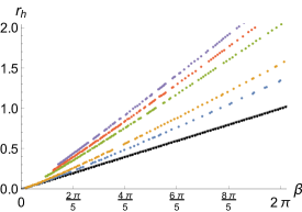
(a) $d=2$, $\Delta=\frac{3}{2}$

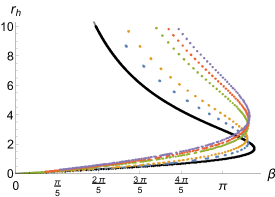
(b) $d=3$, $\Delta=2$

Figure 1: Plots of the horizon radius $r_{\text{h}}$ versus inverse temperature $\beta$ with $\ell=1$ and for both (a) $d=2$, $\Delta=\frac{3}{2}$ and (b) $d=3$, $\Delta=2$. We plot these points for various different values of the deformation parameter $\phi_{0}\pm 0.5\%$. For $d=2$, we observe a one-to-one linear relationship, indicating that each temperature corresponds to just a single black hole in the bulk. For $d=3$ however, there are two solutions for each $\beta$—a large black hole (the lower branches) and a small black hole (the upper branches). As a sanity check, we note the $\phi_{0}\approx 0$ numerical points are consistent with known analytic expressions for $r_{\text{h}}$, which are $\frac{\beta}{2\pi}$ for $d=2$ and $\frac{2\pi}{\beta}\pm\sqrt{\left(\frac{2\pi}{\beta}\right)^{2}-3}$ (resp. the small and large branches) for $d=3$.

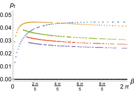
(a) $d=2$, $\Delta=\frac{3}{2}$

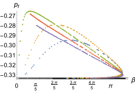
(b) $d=3$, $\Delta=2$

Figure 2: Plots of the Kasner exponent $p_{t}$ versus inverse temperature $\beta$ with $\ell=1$ and for both (a) $d=2$, $\Delta=\frac{3}{2}$ and (b) $d=3$, $\Delta=2$. We again plot these points for various different values of the deformation parameter $\phi_{0}\pm 0.5\%$. For both, the $\phi_{0}\approx 0$ values of $p_{t}$ are only fixed by the dimension (55) and thus respectively are $0$ and $-\frac{1}{3}$. For $\phi_{0}\not\approx 0$, the $d=2$ plot is a well-defined function whereas the $d=3$ plot is branched. In the latter, the upper branch corresponds to large black holes while the lower branch corresponds to small black holes.

With that in mind, for each of these families of black holes we also plot $p_{t}$ as a function of the inverse temperature in Figure 2. For both $d=2$ and $d=3$, we see that the vacuum Kasner exponent $p_{t}|_{\text{vac}}=-1+\frac{2}{d}$ (55) are reproduced by our numerics. With a deformation turned on however, $p_{t}$ develops a nontrivial relationship with $\beta$.

For $d=2$, we get a fairly consistent functional structure (at least for low $\phi_{0}$, but we expect it to hold for larger $\phi_{0}$). $p_{t}$ apparently increases from the vacuum value of $0$ for small $\beta$ until reaching a maximum value dependent on $\phi_{0}$, and then decreases. We may even posit that the value of $\beta$ at this maximum decreases with $\phi_{0}$.

Meanwhile for $d=3$, the presence of two black holes for each $\beta$ manifests branching in Figure 2b. More specifically, we observe that the small black holes have Kasner exponents much closer to the vacuum value than than those of the large black holes. In other words, the small black holes are the lower branch of Figure 2b, while the large black holes exhibit a similar behavior to those of $d=2$ with a spinodal point present. One way to interpret this is to say that small black holes have “more” near-singularity geometry, since as per (56) $g_{tt}$ would blow-up more for small black holes.

So to summarize, deformations of the UV turn on nontrivial relationships between UV and trans-IR data. In particular, the near-singularity geometry is no longer completely specified by $d$. We now want to describe such relationships in terms of other parameters of the UV CFT that are directly connected to phase transitions of holographic quantities.

4 Imprints of entanglement plateaux

One phase transition unique to the round black hole concerns holographic entanglement entropy as computed by the Ryu–Takayanagi (RT) prescription Ryu:2006bv; Hubeny:2007xt, which we now summarize. First, consider a bulk codimension-2 surface $\Gamma$ which is “homologous” to $\mathcal{R}$ ($\Gamma\sim\mathcal{R}$), by which we mean that there exists a codimension-1 bulk region $\Sigma$ for which

$$\partial\Sigma=\mathcal{R}\cup\Gamma,\ \ \partial\mathcal{R}=\partial\Gamma,$$ (57)

Then, to leading order in a small (in units of AdS radius) $G_{\text{N}}$ expansion, the entanglement entropy of a boundary interval $\mathcal{R}$ on a fixed-time slice is proportional to the area of the smallest such $\Gamma$:

$$S(\mathcal{R})=\,\stackrel{{\scriptstyle[}}{{\Gamma}}\sim\mathcal{R}]{}{\text{min}\,\text{ext}}\left[\frac{\text{Area}(\Gamma)}{4G_{\text{N}}}\right].$$ (58)

The minimal-area extremal surface is called the RT surface.

In simple cases like pure AdS or the planar AdS-Schwarzschild black hole, the RT surface is connected if $\mathcal{R}$ is connected. However, this need not be the case in the round black hole (as also appreciated in other work Headrick:2007km; Azeyanagi:2007bj; Blanco:2013joa). For example, when $\mathcal{R}$ constitutes a sufficiently large connected subregion of the boundary in a higher-dimensional ($d>2$) round AdS black hole, one does not even have connected homologous extremal surfaces as candidates for the RT surface in the first place Hubeny:2013gta! The relevant feature of a round black hole is that any bulk region $\Sigma$ bounded by a sufficiently large $\mathcal{R}$ and some extremal connected surface always includes the horizon, so it must be included as a separate connected component of the RT surface. Indeed, allowing for disconnected $\Gamma$ is the only way to have the RT prescription be continuous with the Bekenstein–Hawking formula Bekenstein:1973ur; Hawking:1976de in the limit where $\mathcal{R}$ is the full boundary, for which the RT surface should only be the horizon.

As a generic adaptation of the RT prescription to round black holes, Hubeny:2013gta starts by considering two separate classes of codimension-2 surfaces homologous to $\mathcal{R}$—those which are connected and those which are disconnected and include the horizon. See Figure 3 for a visual representation. Then, computing the entanglement entropy amounts to finding the minimum-area extremal surface among both classes:

$$S(\mathcal{R})=\text{min}\left[\frac{\text{Area}(\Gamma_{\text{C}})}{4G_{\text{N}}},\frac{\text{Area}(\Gamma_{\text{D}})}{4G_{\text{N}}}\right]=\text{min}\left(S_{\text{C}},\,\overline{S}_{\text{D}}+S_{\text{BH}}\right).$$ (59)

Figure 3: A fixed-time slice of the round black hole, with the RT candidates corresponding to a boundary region $\mathcal{R}$. Generically, the true minimal RT surface may either be connected ($\Gamma_{\text{C}}$) or disconnected ($\Gamma_{\text{D}}$). Note that $\Gamma_{\text{D}}$ itself has two connected components—a piece $\overline{\Gamma}_{\text{D}}$ that wraps around the black hole horizon and the horizon itself.

In the equation above, $\Gamma_{\text{C}}$ denotes a generic extremal surface which is both connected and homologous to $\mathcal{R}$. The area of this surface is directly related to $S_{\text{C}}$. Meanwhile $\Gamma_{\text{D}}$ is the extremal surface which is disconnected and homologous to $\mathcal{R}$. It helps to break the resulting entropy into two terms, each corresponding to a connected component of $\Gamma_{\text{D}}$. The first term $\overline{S}_{\text{D}}$ is computed by the connected component $\overline{\Gamma}_{\text{D}}\subset\Gamma_{\text{D}}$ which is anchored to the conformal boundary and wraps around the horizon. The second term $S_{\text{BH}}$ is the Bekenstein–Hawking entropy of the horizon itself.

That there are two competing candidates in the round black hole allows for a first-order phase transition as described in Hubeny:2013gta. First, recall that if the full system is in a pure state, then the entanglement entropy of any subregion $\mathcal{R}$ and its complement $\mathcal{R}^{c}$ must match. For mixed states, we may quantify the “deviation” from this purity as

$$\delta S_{\mathcal{R}}=S(\mathcal{R})-S(\mathcal{R}^{c}).$$ (60)

By the Araki–Lieb inequality (cf. Theorem 2c of Araki:1970ba),

$$|\delta S_{\mathcal{R}}|\leq S(\mathcal{R}\cup\mathcal{R}^{c})=S_{\text{BH}},$$ (61)

where the entropy of the full boundary system is equated to the Bekenstein–Hawking entropy. Saturation of the Araki–Lieb inequality corresponds to a canonical factorization of the full boundary degrees of freedom, with any of the resulting factors carrying all of the microscopic entanglement entropy (cf. Theorem III.2 of Zhang_2011).

We may analyze the deviation from purity on the left-hand side of (61) as we tune the “size” (we make this more precise below) of $\mathcal{R}$ from $0$ to half of the full boundary interval. In doing so, we find that for small $\mathcal{R}$ there is a window of interval sizes for which $S_{\mathcal{R}}$ and $S_{\mathcal{R}^{c}}$ are respectively computed by $\Gamma_{\text{C}}$ and $\Gamma_{\text{C}}\cup\Gamma_{\text{h}}$, where $\Gamma_{\text{h}}$ is the horizon. For $\mathcal{R}$ near half of the boundary, however, there is another window of interval sizes for which both entropies are computed by corresponding connected phases ($\Gamma_{C}$ and $\overline{\Gamma}_{D}$, respectively). According to (59), these two windows are respectively described by

$$S_{\text{C}}\leq\overline{S}_{\text{D}}-S_{\text{BH}} \implies|\delta S_{\mathcal{R}}|=S_{\text{BH}},$$ (62)

$$\overline{S}_{\text{D}}-S_{\text{BH}}<S_{\text{C}}\leq\overline{S}_{\text{D}} \implies 0\leq|\delta S_{\mathcal{R}}|<S_{\text{BH}}.$$ (63)

If we plot $|\delta S_{\mathcal{R}}|$ as a function of interval size, we observe a so-called entanglement “plateau” Hubeny:2013gta. The fall from the plateau corresponds to loss of saturation of the Araki–Lieb inequality.

We aim to understand how this phase transition imprints upon the trans-IR Kasner exponents. To do so, we take $\mathcal{R}$ to be a round “cap” [with $SO(d-1)$ symmetry] in the boundary whose size is controlled by a single angular parameter $\theta_{\mathcal{R}}$. The transition is found to occur at a particular $\theta_{\mathcal{R}}=\theta_{\text{k}}$. With a scalar deformation in the UV, we find that this transition point can be viewed as UV data in lieu of the CFT temperature parameter $\frac{\beta}{\ell}$ in the list (42). With that in mind, we plot $\theta_{\text{k}}$ against the Kasner exponent $p_{t}$ at fixed values of the deformation parameter $\phi_{0}\ell^{d-\Delta}$.

As a matter of practicality, we focus on the $d=2$ case for which the extremal surfaces can be computed from a first-order ODE. The higher-dimensional cases are in principle possible to analyze, but they require numerically solving second-order ODEs. We discuss the basic machinery of general $d\geq 2$ in Appendix LABEL:app:entropyCaps, leaving the higher-dimensional problem open for future work.

Essentially, we will find that a finite, nonzero deformation induces a nontrivial relationship between $p_{t}$ and $\theta_{\text{k}}$. The takeaway is that a deformation allows entanglement structure in the UV to imprint upon the trans-IR data (at least in the low-dimensional case of $d=2$). We find that this effect is numerically small.

4.1 Ryu–Takayanagi in deformations of the BTZ black hole

We compute entanglement plateaux for deformations of the round BTZ black hole in $d=2$, which is described by the metric (fixing the curvature radius as $\ell=1$)

$$ds^{2}=\frac{1}{r^{2}}\left[-e^{-\chi(r)}F(r)dt^{2}+\frac{dr^{2}}{F(r)}+d\theta^{2}\right],$$ (64)

with $t\in\mathbb{R}$, $r>0$, and $\theta\sim\theta+2\pi$. Recall that we assume $F$ to have a simple root at $r=r_{\text{h}}$, defined as the black hole horizon. Furthermore, it is convenient to take the fundamental domain $\theta\in(-\pi,\pi]$, with $\mathcal{R}$ at fixed time being parameterized as $\theta\in[-\theta_{\mathcal{R}},\theta_{\mathcal{R}}]$ for some $0<\theta_{\mathcal{R}}<\frac{\pi}{2}$. Our goal will be to find the value $\theta_{\mathcal{R}}=\theta_{\text{k}}$ at which the Araki–Lieb inequality switches between being saturated and holding strictly.

To compute the extremal surfaces, we first use the metric to write the area functional of a surface $\theta=\theta(r)$ at fixed $t$ (omitting bounds of integration for now)

$$\mathcal{A}=\int\frac{dr}{r}\sqrt{\frac{1}{F(r)}+\theta^{\prime}(r)^{2}}.$$ (65)

We then use the Euler-Lagrange equation to obtain the equation of motion for the extremal surfaces,

$$\theta^{\prime}(r)^{2}=\frac{r^{2}}{F(r)(r_{*}^{2}-r^{2})},$$ (66)

Here, $r_{*}<r_{\text{h}}$ is a bulk constant of motion characterizing the turnaround point of the extremal surface, i.e., $\frac{dr}{d\theta}|_{r=r_{*}}=\frac{1}{\theta^{\prime}(r_{*})}=0$ and $r\in[0,r_{*}]$. By integrating (66), we can relate this $r_{*}$ parameter to $\theta_{\mathcal{R}}$.

We now have the necessary expressions to compute the areas of the RT candidates for both $\mathcal{R}$ and $\mathcal{R}^{c}$. Before we proceed, we reiterate that $\Gamma_{\text{C}}$ denotes the connected extremal surface homologous to $\mathcal{R}$ while the homologous disconnected extremal surface $\Gamma_{\text{D}}$ decomposes into connected components $\overline{\Gamma}_{\text{D}}\cup\Gamma_{\text{h}}$, where $\Gamma_{\text{h}}$ is the horizon and $\partial\overline{\Gamma}_{\text{D}}=\partial\mathcal{R}$. We observe that the connected phase for the entropy of the complement $\mathcal{R}^{c}$ is then computed by the connected component $\overline{\Gamma}_{\text{D}}$, and the disconnected phase is computed by the union $\Gamma_{\text{C}}\cup\Gamma_{\text{h}}$. So at this stage, we simply need to compute the endpoints and areas of $\Gamma_{\text{C}}$ and $\overline{\Gamma}_{\text{D}}$ in terms of their turnaround points.

Computing $\Gamma_{\text{C}}$

We first relate the turnaround point $r_{\text{c}*}$ of $\Gamma_{\text{C}}$ to $\theta_{\mathcal{R}}$. To start, note that $\Gamma_{\text{C}}$ represents a surface which does not wrap around the black hole horizon relative to $\mathcal{R}$ (Figure 3). Therefore, the $\theta(r)>0$ branch has the negative root of (66) as its derivative, so we write

$$\theta(r_{\text{c}*})-\theta(0)=-\int_{0}^{r_{\text{c}*}}\frac{dr}{\sqrt{F(r)}}\frac{r}{\sqrt{r_{\text{c}*}^{2}-r^{2}}}.$$ (67)

By the symmetry of our parameterization, $\theta(r_{\text{c}*})=0$. Additionally, $\theta(0)=\theta_{\mathcal{R}}$. As such, we have

$$\theta_{\mathcal{R}}=\int_{0}^{r_{\text{c}*}}\frac{dr}{\sqrt{F(r)}}\frac{r}{\sqrt{r_{\text{c}*}^{2}-r^{2}}}.$$ (68)

Furthermore, the area of $\Gamma_{\text{C}}$ may be written by plugging (66) directly into (65):

$$\text{Area}(\Gamma_{\text{C}})=2\int_{0}^{r_{\text{c}*}}\frac{dr}{\sqrt{F(r)}}\frac{r_{\text{c}*}/r}{\sqrt{r_{\text{c}*}^{2}-r^{2}}}.$$ (69)

Computing $\overline{\Gamma}_{\text{D}}$

We now relate the turnaround point $r_{\text{d}*}$ of $\overline{\Gamma}_{\text{D}}$ to $\theta_{\mathcal{R}}$. As shown in Figure 3, this surface wraps around the black hole horizon relative to $\mathcal{R}$. As such, the derivative of the $\theta(r)>0$ branch is the positive root of (66), so

$$\theta(r_{\text{d}*})-\theta(0)=\int^{r_{\text{d}*}}_{0}\frac{dr}{\sqrt{F(r)}}\frac{r}{\sqrt{r_{\text{d}*}^{2}-r^{2}}}.$$ (70)

This time, we have that $\theta(r_{\text{d}*})=\pi$ and $\theta(0)=\theta_{\mathcal{R}}$. Hence,

$$\theta_{\mathcal{R}}=\pi-\int_{0}^{r_{\text{d}*}}\frac{dr}{\sqrt{F(r)}}\frac{r}{\sqrt{r_{\text{d}*}^{2}-r^{2}}}.$$ (71)

However, the area of $\overline{\Gamma}_{\text{D}}$ takes the same form as that of $\Gamma_{\text{C}}$,

$$\text{Area}(\overline{\Gamma_{D}})=2\int_{0}^{r_{\text{d}*}}\frac{dr}{\sqrt{F(r)}}\frac{r_{\text{d}*}/r}{\sqrt{r_{\text{d}*}^{2}-r^{2}}}.$$ (72)

Applying Ryu–Takayanagi

For a fixed $\mathcal{R}$ (and $\mathcal{R}^{c}$), we can in principle use the simultaneous constraints (68) and (71) to solve for the turnaround points $r_{\text{c}*}$ and $r_{\text{d}*}$ in terms of the interval size parameter $\theta_{\mathcal{R}}$. With those in hand, we can then plug the expressions (69) and (72) into the holographic prescriptions for the entanglement entropies of $\mathcal{R}$ and $\mathcal{R}^{c}$ to evaluate the entropies:

$$S(\mathcal{R}) =\frac{1}{4G_{\text{N}}}\text{min}\left[\text{Area}(\Gamma_{\text{C}}),\,\text{Area}(\overline{\Gamma}_{\text{D}})+\frac{2\pi}{r_{\text{h}}}\right],$$ (73)

$$S(\mathcal{R}^{c}) =\frac{1}{4G_{\text{N}}}\text{min}\left[\text{Area}(\Gamma_{\text{C}})+\frac{2\pi}{r_{\text{h}}},\,\text{Area}(\overline{\Gamma}_{\text{D}})\right].$$ (74)

The $\frac{2\pi}{r_{\text{h}}}$ term is the horizon area in the $d=2$ round black hole and notably does not depend on the deformation. With these equations, we may compute the absolute difference of entropies $|\delta S_{\mathcal{R}}|=|S(\mathcal{R})-S(\mathcal{R}^{c})|$ explicitly. By scanning over $\theta_{\mathcal{R}}$, we can plot $|\delta S_{\mathcal{R}}|$ as a function of interval size, and it is in such plots that we identify entanglement plateaux.

That being said, we know that the transition in entropy occurs between the windows (62) and (63), i.e.,

$$\theta_{\mathcal{R}}=\theta_{\text{k}}\iff S_{\text{C}}=\overline{S}_{\text{D}}-S_{\text{BH}}\iff\frac{2\pi}{r_{\text{h}}}=\text{Area}(\overline{\Gamma}_{\text{D}})-\text{Area}(\Gamma_{\text{C}}).$$ (75)

This along with (68) and (71) completely constrain the transition point and can be used to find the transition value $\theta_{\mathcal{R}}=\theta_{\text{k}}$ without needing to plot $|\delta S_{\mathcal{R}}|$.

4.2 Plateaux kinks versus Kasner exponents

Given some solution to the equations of motion with horizon radius $r=r_{\text{h}}$, we reiterate that the respective turnaround points $r_{\text{c}*}$ and $r_{\text{d}*}$ of $\Gamma_{\text{C}}$ and $\overline{\Gamma}_{\text{D}}$ at the transition angle $\theta_{\mathcal{R}}=\theta_{\text{k}}$ are fixed by the following system of constraints:

$$\theta_{\text{k}} =\int_{0}^{r_{\text{c}*}}\frac{dr}{\sqrt{F(r)}}\frac{r}{\sqrt{r_{\text{c}*}^{2}-r^{2}}},$$ (76)

$$\theta_{\text{k}} =\pi-\int_{0}^{r_{\text{d}*}}\frac{dr}{\sqrt{F(r)}}\frac{r}{\sqrt{r_{\text{d}*}^{2}-r^{2}}},$$ (77)

$$\frac{\pi}{r_{\text{h}}} =\int_{0}^{r_{\text{d}*}}\frac{dr}{\sqrt{F(r)}}\frac{r_{\text{d}*}/r}{\sqrt{r_{\text{d}*}^{2}-r^{2}}}-\int_{0}^{r_{\text{c}*}}\frac{dr}{\sqrt{F(r)}}\frac{r_{\text{c}*}/r}{\sqrt{r_{\text{c}*}^{2}-r^{2}}}.$$ (78)

To use these constraints, we first obtain a large number of numerical solutions to the equations of motion (36)–(38). We then scan for fixed values of the deformation parameter $\phi_{0}$ (with some prescribed uncertainty) and, for this subset of solutions, numerically solve the above constraints. After post hoc validation that the numerical output indeed solves these constraints, we are left with the desired values of $\theta_{\text{k}}$. We can then check whether $\theta_{\text{k}}$ is a monotonic function of $\beta$, thereby allowing us to substitute the latter for the former in the UV data without issue. We then plot the Kasner exponent $p_{t}$ against $\theta_{\text{k}}$.

Before discussing the numerics, however, we note that the case of the (undeformed) BTZ black hole can be understood analytically. We do so both as a warm-up and to have a consistency test in hand for our numerics.

Undeformed BTZ

Let us review the case of the BTZ black hole in pure gravity, also analyzed by Hubeny:2013gta. As it turns out, the interval size corresponding to the plateau of the BTZ can be computed analytically. First, recall that

$$F_{\text{BTZ}}(r)=1-\frac{r^{2}}{r_{\text{h}}^{2}}.$$ (79)

This can be used to compute both $r_{\text{c}*}$ and $r_{\text{d}*}$ as functions of $\theta_{\mathcal{R}}$:

$$r_{\text{c}*}^{\text{BTZ}} =r_{\text{h}}\tanh\left(\frac{\theta_{\mathcal{R}}}{r_{\text{h}}}\right),$$ (80)

$$r_{\text{d}*}^{\text{BTZ}} =r_{\text{h}}\tanh\left(\frac{\pi-\theta_{\mathcal{R}}}{r_{\text{h}}}\right).$$ (81)

Now, we want to compute the interval size $\theta_{\mathcal{R}}\equiv\theta_{\text{k}}^{\text{BTZ}}$ defining the kink of the plateau. Recalling (62)–(63), this is found by setting

$$\text{Area}(\overline{\Gamma}_{\text{D}})-\text{Area}(\Gamma_{\text{C}})=\frac{2\pi}{r_{\text{h}}}.$$ (82)

For the BTZ geometry, we can compute each of these areas, and thus $\theta_{\text{k}}^{\text{BTZ}}$, analytically. First, define a regulator surface $r=\epsilon$. The regulated areas are then

$$\text{Area}(\Gamma_{\text{C}})_{\text{BTZ}}^{\text{reg}} =-2\log\left(\frac{\epsilon}{2r_{h}}\right)+\log\left(\frac{r_{\text{c}*}^{2}}{r_{\text{h}}^{2}-r_{\text{c}*}^{2}}\right),$$ (83)

$$\text{Area}(\overline{\Gamma}_{\text{D}})_{\text{BTZ}}^{\text{reg}} =-2\log\left(\frac{\epsilon}{2r_{h}}\right)+\log\left(\frac{r_{\text{d}*}^{2}}{r_{\text{h}}^{2}-r_{\text{d}*}^{2}}\right).$$ (84)

The UV divergences manifestly cancel when we take the difference, so the constraint (82) is well-defined and yields the following relation:

$$\theta_{\text{k}}^{\text{BTZ}}=\frac{\pi}{2}-\frac{r_{\text{h}}}{2}\log\cosh\left(\frac{\pi}{r_{\text{h}}}\right).$$ (85)

The horizon temperature (20) of the BTZ black hole is $T_{\text{h}}=\frac{1}{2\pi r_{\text{h}}}$, so we may write the kink angle as a monotonic function of the inverse CFT temperature $\beta=T_{\text{h}}^{-1}$,

$$\theta_{\text{k}}^{\text{BTZ}}=\frac{\pi}{2}\left[1-\frac{\beta}{2\pi^{2}}\log\cosh\left(\frac{2\pi^{2}}{\beta}\right)\right].$$ (86)

So the value of $\theta_{\text{k}}^{\text{BTZ}}$ depends on the temperature (or size through $\beta\sim r_{\text{h}}$) of the black hole. For high-temperature ($\beta\to 0$) and low-temperature ($\beta\to\infty$) BTZ black holes,

$$\lim_{\beta\to 0}\theta^{\text{BTZ}}_{\text{k}}=0,\ \ \lim_{\beta\to\infty}\theta^{\text{BTZ}}_{\text{k}}=\frac{\pi}{2}.$$ (87)

In other words, for large black holes $r_{\text{h}}\ll 1$ there is effectively no range for which the Araki–Lieb inequality is saturated, whereas for small black holes $r_{\text{h}}\gg 1$ the Araki–Lieb inequality is effectively always saturated. However, we may also consider intermediate regimes at which the transition happens at finite interval size, as shown in Figure 4.

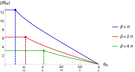
Figure 4: Exact entanglement plateaux for the BTZ black hole (with $\ell=1$) for inverse temperatures $\beta=\pi$ (blue), $\beta=2\pi$ (red), and $\beta=4\pi$ (green). The kinks in each plot are the points at which the phase of $\delta S_{\mathcal{R}}$ (computed via the RT prescription and with $4G_{\text{N}}=1$) changes. These respectively occur at $\theta_{\mathcal{R}}\approx 0.055\pi$, $\theta_{\mathcal{R}}\approx 0.110\pi$, and $\theta_{\mathcal{R}}\approx 0.207\pi$.

Lastly, we emphasize that the Kasner exponent for any black hole solution to the vacuum equations of motion is given by a temperature-independent constant. For BTZ,

$$p_{t}^{\text{BTZ}}=0.$$ (88)

This can be seen by taking $d=2$ in (55). The kinks thus constitute a line at $0$ in the parameter space $(\theta_{\text{k}},\phi_{0},p_{t})$ on the $\phi_{0}=0$ slice (at zero deformation parameter). In other words, the entanglement plateau transition does not imprint upon the interior geometry of the BTZ in the absence of matter.

Finite deformations

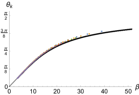
(a) $\theta_{\text{k}}$ versus $\beta$

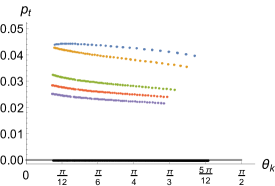
(b) $p_{t}$ versus $\theta_{\text{k}}$

Figure 5: The plots of (a) $\theta_{\text{k}}$ versus $\beta$ and (b) $p_{t}$ versus $\theta_{\text{k}}$ for a variety of scalar deformations characterized by the values of $\phi_{0}$. As our numerics do not find solutions for fixed $\phi_{0}$ outright, we compute these points while allowing for a $0.5\%$ margin of error in the values of $\phi_{0}$. As a sanity check, we numerically compute parameters from solutions with $\phi_{0}\leq 0.005$ (close to $0$) and find that they indeed replicate the analytic results of the undeformed BTZ. The relationship between $\theta_{\text{k}}$ and $\beta$ appears insensitive to the deformation and shows strong matching to the analytic result for $\phi=0$ (86). However, $p_{t}$ develops a nontrivial relationship with $\theta_{\text{k}}$ when $\phi_{0}\not\approx 0$, in contrast to $p_{t}$ being uniformly $0$ when $\phi_{0}\approx 0$.

For the BTZ, there is no relationship between $\theta_{\text{k}}$ (viewed as UV data) and the constant $p_{t}$ (the trans-IR data). Our goal now is to see whether this changes for finite values of the deformation parameter (in $\ell=1$ units). This requires numerics. To summarize our results, we plot both $\theta_{\text{k}}$ versus $\beta$ and $p_{t}$ versus $\theta_{\text{k}}$ from points obtained via our numerical approach for a variety of deformations in Figure 5.

As validation, we first plot the points for $\phi_{0}\leq 0.005$. These points should and do generally follow the analytic relations above, namely (86) for $\theta_{\text{k}}$ versus $\beta$ and a flat line at $0$ for $p_{t}$ versus $\theta_{\text{k}}$. Subsequently, we then plot points for finite values of $\phi_{0}$, namely $\phi_{0}=5.000\pm 0.025$, $10.00\pm 0.05$, $50.00\pm 0.25$, $100.0\pm 0.5$, and $200.\pm 1$—allowing for errors of $0.5\%$ in our scan over deformation parameters.

Just as for the undeformed BTZ, $\theta_{\text{k}}$ monotonically increases in $\beta$, so we can swap $\theta_{\text{k}}$ for the temperature in the UV data. Interestingly, while we certainly observe a dependence of this curve on $\phi_{0}$, it appears to be very small. However, the relationship between $p_{t}$ and $\theta_{\text{k}}$ is much more subtle. Qualitatively, the plot appears stable against the $\pm 0.5\%$ error in $\phi_{0}$. Thus the numerics suggest that for finite, fixed deformations, $\theta_{\text{k}}$ has a numerically weak but nontrivial relationship with $p_{t}$. This is in contrast to no deformation being turned on ($\phi_{0}\approx 0$), in which case $p_{t}$ is completely independent of $\theta_{\text{k}}$. The $\phi_{0}\approx 5$ plot in particular suggests that the Kasner exponent peaks at some value of $\theta_{\text{k}}$. The higher values of $\phi_{0}$ are consistent with this behavior, assuming that their peaks appear at smaller values of $\theta_{\text{k}}$.

These plots reflect how the UV entanglement plateau transition imprints upon the trans-IR data. Physically, both large and small values of $\theta_{\text{k}}$ appear to induce smaller values of $p_{t}$ within the range of our numerics. Thus, there is a particular black hole with maximal $p_{t}$ whose plateau occurs at an intermediate value of $\theta_{\text{k}}$. As per the interpretation of positive $p_{t}$ discussed in Section 3.2, the interior geometry of this dual black hole has a maximally fast collapse relative to other states.

5 Thermal two-point functions and the interior

Another entry of the holographic dictionary involving classical geometry is geodesic approximation of correlation functions. In this section, we restrict our attention to scalar correlation functions, so we assume the presence of a second bulk scalar field ${\widetilde{\Phi}}$ dual to some CFT operator ${\widetilde{\mathcal{O}}}$ in the boundary theory with conformal dimension ${\widetilde{\Delta}}$. Furthermore, for simplicity we assume that this scalar field is not coupled to anything, so it does not generate any gravitational backreaction. We will eventually take ${\widetilde{\Delta}}$ to be large (meaning that ${\widetilde{\mathcal{O}}}$ will be irrelevant), so the presence of ${\widetilde{\Phi}}$ stands in contrast to the scalar $\Phi$ in (32) whose backreaction effects correspond to RG flow from the UV to the trans-IR.

The basic idea of geodesic approximation comes from seminal work equating the scalar propagator of a holographic CFT to a path integral over worldlines in the bulk Banks:1998dd; Balasubramanian:1999zv. Specifically, taking two boundary points $\hat{x}_{1}$ and $\hat{x}_{2}$, the Euclidean scalar propagator is

$$G(\hat{x}_{1},\hat{x}_{2})=\int_{\hat{x}_{1}\leftrightarrow\hat{x}_{2}}\mathcal{D}\mathcal{P}\,e^{-{\widetilde{\Delta}}L[\mathcal{P}]}.$$ (89)

Here, $\mathcal{P}$ is a generic bulk path connecting the boundary points, and $L[\mathcal{P}]$ is a length functional. Given a particular bulk geometry, the left-hand side is equivalent to the Euclidean two-point function of ${\widetilde{\mathcal{O}}}$ in the corresponding CFT state.

Now, we take the limit ${\widetilde{\Delta}}\to\infty$ by taking the bulk scalar mass to be large in units of AdS radius. Hereafter, we denote this large conformal dimension as $\Delta_{\text{H}}$ and the corresponding operator as $\mathcal{O}_{\text{H}}$. The path integral in (89) may then be evaluated using saddle-point approximation. This picks out minima of the length functional—in other words, geodesics:

$$\expectationvalue{\mathcal{O}_{\text{H}}(\hat{x}_{1})\mathcal{O}_{\text{H}}(\hat{x}_{2})}\sim\sum_{\text{geodesics}}e^{-\Delta_{\text{H}}L}.$$ (90)

We can actually go a bit further when working strictly in the $\Delta_{\text{H}}\to\infty$ limit. The sum above is dominated by the minimum-length saddle, and so among the different geodesics there is one in particular that actually determines the two-point function:

$$⟨𝒪{}_{\text{H}}(\widehat{x}{}_1)𝒪{}_{\text{H}}(\widehat{x}{}_2)⟩\sim \exp [-\mathrm{\Delta }{}_{\text{H}}(\stackrel{[}{}geodesics]\text{min}L)].Withthatsaid,weexaminethegeodesicsinone-sidedroundblackholes.Thisisequivalenttocomputingheavy\text{thermal}two-pointfunctions.WeemphasizethatthestudyofgeodesicstogleaninsightintothermalcorrelationfunctionsinCFTisnotnew\text{<cite class="ltx\_cite ltx\_citemacro\_cite"><span class="ltx\_ref ltx\_missing\_citation ltx\_ref\_self">Fidkowski:2003nf</span></cite>}andhasbeenrecentlyrevitalized\text{<cite class="ltx\_cite ltx\_citemacro\_cite"><span class="ltx\_ref ltx\_missing\_citation ltx\_ref\_self">Grinberg:2020fdj</span>; <span class="ltx\_ref ltx\_missing\_citation ltx\_ref\_self">Berenstein:2022nlj</span></cite>}.Ourgoalistoexaminethephasestructureoftheseheavythermaltwo-pointfunctionsoncompactspatialslices.Inparticular,weconsideraCFTthermalstateonS{}^{d-1}andnotethattwooperatorinsertionswillalwaysbecollinear.Thus,thepicturelookssimilartoFigure\text{<a href="\#S4.F3" title="Figure 3 ‣ 4 Imprints of entanglement plateaux ‣ Imprints of phase transitions on Kasner singularities" class="ltx\_ref ltx\_font\_italic"><span class="ltx\_text ltx\_ref\_tag">3</span></a>},withtwodifferentconnectedgeodesicsbeingamongthepossibledominantphasesofthetwo-pointfunction.Ifeitherdominatesthegeodesicapproximation,thenwehaveaconnectedtwo-pointfunction.Inaddition,thereisathirdcandidate---adisconnectedpairofgeodesics,eachofwhichisanchoredtooneoftheinsertionsandhitsthehorizon.Thisthirdcandidaterepresentsthedisconnectedpartofthetwo-pointfunction(theproductoftheheavythermalone-pointfunctions\text{<cite class="ltx\_cite ltx\_citemacro\_cite"><span class="ltx\_ref ltx\_missing\_citation ltx\_ref\_self">Grinberg:2020fdj</span></cite>}).Thethreegeodesicswhichcontributetothethermaltwo-pointfunctionareshowninFigure\text{<span class="ltx\_ref ltx\_missing\_label ltx\_font\_italic ltx\_ref\_self">LABEL:figs:round2pt</span>}.\text{Figure 6Figure 66Figure 6D∙∙∘∘OHOHOHOHC1C26Afixed-timesliceoftheroundblackhole(inLorentziansignature),withthetwoconnectedgeodesi}$$ (91)