More powerful multiple testing under dependence
via randomization

Abstract

We show that two procedures for false discovery rate (FDR) control — the Benjamini-Yekutieli procedure for dependent p-values, and the e-Benjamini-Hochberg procedure for dependent e-values — can both be made more powerful by a simple randomization involving one independent uniform random variable. As a corollary, the Hommel test under arbitrary dependence is also improved. Importantly, our randomized improvements are never worse than the originals, and they are typically strictly more powerful, with marked improvements in simulations. The same technique also improves essentially every other multiple testing procedure based on e-values.

1 Introduction

In the multiple testing problem, we wish to test $K$ hypotheses, out of which an unknown subset $\mathcal{N}\subseteq[K]\coloneqq\{1,\dots,K\}$ contains those where the null hypothesis is actually true. Let $\mathcal{D}$ denote the set of rejections (“discoveries”) made by a multiple testing procedure. Then, $\mathcal{N}\cap\mathcal{D}$ are the “false discoveries”. The false discovery rate (FDR) is defined as follows:

$$\mathrm{FDR}\coloneqq\mathbb{E}\left[\frac{|\mathcal{D}\cap\mathcal{N}|}{|\mathcal{D}|\vee 1}\right],$$ (2)

where $a\vee b:=\max(a,b)$. The goal of an FDR controlling multiple testing method is to always ensure $\mathrm{FDR}\leq\alpha$ for a predefined level $\alpha\in(0,1)$.

One of the seminal results in multiple testing under arbitrary dependence was developed by Benjamini and Yekutieli (2001). They showed that if the $K$ input p-values are arbitrarily dependent, then the Benjamini-Hochberg (BH) procedure (Benjamini and Hochberg, 1995) is only guaranteed to control the false discovery rate (FDR) if it is run at the target level $\alpha$ divided by an approximately $\log K$ factor. We refer to this more conservative version of the BH procedure — which still ensures FDR control under arbitrary dependence — as the BY procedure. The BY procedure is known to be unimprovable in the sense that there is an “extreme” example for which it achieves FDR equal to $\alpha$ (Guo and Bhaskara Rao, 2008). Here, we show the surprising fact that outside of this extreme example, its power can be (usually strictly) improved using independent, external randomization.

Despite the above procedure using only p-values and having nothing to do with “e-values”, the key idea for its improvement stems from the latter concept. In particular, our technique involves a simple stochastic rounding of e-values.

A random variable $X$ is an e-value iff $X$ is nonnegative $\mathbb{E}[X]\leq 1$ under the null hypothesis. E-values have been recognized as a powerful tool for hypothesis testing in the last few years (Wasserman et al., 2020; Grünwald et al., 2023; Shafer, 2021; Vovk and Wang, 2021; Howard et al., 2020). For example, the universal inference statistic provides an e-value for testing any composite null without regularity conditions (Wasserman et al., 2020); as a result, one can now construct tests using e-values in problems where no prior test was known. One such example is the problem of testing the log-concavity of a distribution; the only known valid test is based on an e-value (Dunn et al., 2022; Gangrade et al., 2023). Many other examples exist (Ramdas et al., 2023).

E-values have a intrinsic connection to anytime-valid inference — “anytime-valid” refers to sequential nature of sampling data, where one can choose when to stop and make an inference based on the collected data. Admissible anytime-valid tests (or confidence intervals) must be derived from e-values (Ramdas et al., 2020).

Recently, Wang and Ramdas (2022) showed that the BY procedure is a special case of the e-BH procedure, which is the e-value analog of the BH procedure for FDR control. Our paper also improves the e-BH procedure using the same randomization technique. To recap the e-BH procedure, let $X_{1},\dots,X_{K}$ be $K$ e-values (testing $K$ different null hypotheses), and define

$$k^{*}\coloneqq\max\left\{k\geq 1:X_{[i]}\geq\frac{K}{k\alpha}\right\},$$ (3)

where $X_{[i]}$ refers to the $k$-th order statistic of the e-values when sorted in decreasing order (so $X_{[i]}$ is the $k$-th largest e-value), and the $\max$ of an empty set is defined as 0. The e-BH procedure rejects the hypotheses corresponding to the $k^{*}$ largest e-values, and we denote this set of discoveries as $\mathcal{D}_{\textnormal{eBH}}$. Wang and Ramdas (2022) showed that the e-BH procedure controls FDR at $\alpha$ under any arbitrary dependence between the e-values (a fact that is not true for the BH procedure based on p-values, which is why the corrected BY procedure is needed).

It turns out that one can view the e-BH procedure as selecting a data-dependent threshold

$$\widehat{\alpha}^{*}\coloneqq\frac{\alpha(k^{*}\vee 1)}{K}$$ (4)

and rejecting (i.e., including in $\mathcal{D}$) the $i$th hypothesis if and only if $X_{i}\geq 1/\widehat{\alpha}^{*}$. Observe that $1/\widehat{\alpha}^{*}$ can only take values from the grid $\{K/(k\alpha):i\in[K]\}$. If we “rounded” down each $X_{i}$ to the closest value in the grid that is less than $X_{i}$ (or 0 if $X_{i}$ is smaller than any value in the grid), the discovery set that is output by e-BH would be identical to the one where no rounding had occurred. But if we could round up the e-value, we would potentially gain power; however this would inflate its expectation and it would no longer be an e-value. Our key insight is that if we randomly rounded every e-value up or down — appropriately so that its expectation is unchanged — then we could increase power with positive probability.

The fact that most e-values will typically lie between grid points provides an opportunity to significantly increase the power. Usually, rounding to the grid would require us to know the true distribution for each $X_{i}$ where the null hypothesis is true (e.g., this is called e-value boosting in Wang and Ramdas (2022)); that is often infeasible, particularly when we are testing composite null hypotheses. In what follows, we develop methods that use independent external randomness to stochastically round e-values, and increase the number of discoveries made by e-BH. This in turn improves the power of the seminal BY procedure.

Summary of contributions

Having explained our new ideas abstractly above, we now concisely highlight the key improvements in multiple testing methodology that we obtain through randomization. In the sequel, let $U$ be a uniform random variable over $[0,1]$ independent of any e-values or p-values.

1. Improving e-BH through stochastic rounding: Our core contribution is a new method based on stochstic rounding, U-eBH, that has the following simple characterization:

   $$\text{Apply BH to }(U/X_{1},\dots,U/X_{K}).$$

   U-eBH dominates the standard e-BH procedure:

   $$\text{Apply BH to }(1/X_{1},\dots,1/X_{K}).$$

   Both procedures retain valid FDR control, which we prove in Theorem 4. Notably, U-eBH strictly improves the discovery set that is rejected by e-BH. This means that the rejections made by e-BH will always be a subset of the rejections produced U-eBH. In addition to U-eBH, we develop a framework for stochastic rounding, and formulate other randomized methods in this framework that all possess this strict improvement property over e-BH.

2. Randomized version of the BY procedure for p-values: We can also improve the BY procedure for multiple testing with FDR control under arbitrary dependence through randomization. Let $(P_{1},\dots,P_{K})$ be $K$ arbitrarily dependent p-values and $P_{(k)}$ denote the $k$th smallest p-value. Both U-BY and BY reject the hypotheses corresponding to the smallest p-values — U-BY makes the following number of discoveries:

   $$k^{*}_{\text{U-\text{BY}}}\coloneqq\max\left\{k\geq 1:P_{(k)}\leq\frac{\alpha\lfloor k/U\rfloor}{K\ell_{K}}\right\}.$$ (5)

   On the other hand, BY only makes the following number of discoveries:

   $$k^{*}_{\text{\text{BY}}}\coloneqq\max\left\{k\geq 1:P_{(k)}\leq\frac{\alpha k}{K\ell_{K}}\right\}.$$ (6)

   Again, the randomized U-BY dominates the deterministic BY and still possesses FDR control, as we show in Theorem 5. Our U-BY procedure also controls the FDR, never makes fewer discoveries than BY, and typically makes many more. This is a result of applying p-to-e calibration alongside our randomized e-value procedures. In addition, we prove a stronger version of the superuniformity lemma for arbitrarily dependent p-values from Blanchard and Roquain (2008) and Ramdas et al. (2019) — thus, we can apply our rounding technique to any multiple testing procedure that uses reshaping functions.

3. Randomized Hommel for global null testing: We can also randomize the Hommel procedure (Simes, 1986) to formulate a randomized U-Hommel p-value that is always upper bounded (i.e., at least as powerful) as the typical Hommel p-value. We extend stochastic rounding to improve any admissible homogeneous p-merging procedure, as characterized by Vovk et al. (2022), in Appendix E. Our randomized U-Hommel procedure and its deterministic analog, the Hommel procedure, are formulated as follows:

   $$P_{{\textnormal{U-Hommel}}}\coloneqq\min_{i\in[K]}\frac{P_{(i)}K\ell_{K}}{(\lfloor i/U\rfloor\wedge K)},\qquad P_{{\textnormal{Hommel}}}\coloneqq\min_{i\in[K]}\frac{P_{(i)}K\ell_{K}}{i}.$$ (7)

   We show that the U-Hommel p-value also possesses Type I error control in Theorem 7 while never being larger and often smaller than the Hommel p-value.

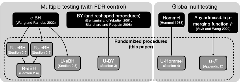
Figure 1: Summary of procedures we improve through randomization in this paper. All randomized procedures retain the validity of their deterministic counterparts, i.e., FDR control for multiple testing and Type I error control for global null testing.

In addition to these improvements, we also provide results on randomizing other methods — a summary of the results in this paper is illustrated in Figure 1. The rest of the paper is organized in the following fashion. In Section 2 we introduce the notion of stochastic rounding, and describe different ways in which it can be combined with the e-BH procedure to improve power. We formulate the U-BY procedure—the randomized version of the BY procedure—in Section 3. Section 4 contains our derivation of the U-Hommel procedure that randomizes the Hommel procedure. In Section 5, we relate our randomization techniques to weighted BH procedures. We show our methods have more power than their deterministic counterparts in numerical simulations in Section 6, and if the sole goal of a practitioner was to maximize power, one should seriously consider using randomization to attain more discoveries.

2 Randomization improves the e-BH procedure

In this section, we show how to (usually strictly) improve the power of the e-BH procedure by stochastically rounding the e-values. This notion lies at the core of our randomized procedures.

2.1 Stochastic rounding of e-values

Define $\mathbb{R}_{+}$ as the nonnegative reals, and $\overline{\mathbb{R}}_{+}\coloneqq\mathbb{R}_{+}\cup\{+\infty\}$, and note the latter is closed set. Consider any closed subset $\mathcal{G}\subseteq\overline{\mathbb{R}}_{+}$ (where $\mathcal{G}$ stands for “grid”, since $\mathcal{G}$ will often be countable or finite below). Denote $g_{*}\coloneqq\inf\{x:x\in\mathcal{G}\}$ and $g^{*}\coloneqq\sup\{x:x\in\mathcal{G}\}$, and note that $g_{*},g^{*}\in\mathcal{G}$ since $\mathcal{G}$ is closed. Further, for any $x\in[g_{*},g^{*}]$, denote

$$x^{+}\coloneqq\inf\{y\in\mathcal{G}:y\geq x\},\qquad x_{-}\coloneqq\sup\{y\in\mathcal{G}:y\leq x\},$$ (8)

and note that $x^{+},x_{-}\in\mathcal{G}$ with $x^{+}\geq x$ and $x_{-}\leq x$, and if $x\notin\mathcal{G}$, then $x_{-}<x<x^{+}$.

Now define the stochastic rounding of $x\in\overline{\mathbb{R}}_{+}$ onto $\mathcal{G}$, denote $S_{\mathcal{G}}(x)$, as follows. If $x<g_{*}$, $x>g^{*}$, $x\in\mathcal{G}$, or $x^{+}=\infty$ then define $S_{\mathcal{G}}(x)=x$. Otherwise, define

$$S_{\mathcal{G}}(x)=\begin{cases}x_{-}\text{ with probability }\frac{x^{+}-x}{x^{+}-x_{-}},\\ x^{+}\text{ with probability }\frac{x-x_{-}}{x^{+}-x_{-}}.\end{cases}$$ (9)

Note that $S_{\mathcal{G}}(x)$ need not lie in $\mathcal{G}$, because if $x$ lies outside the range of $\mathcal{G}$ then it is left unchanged. Also note that when $\mathcal{G}=\overline{\mathbb{R}}_{+}$, we have $S_{\mathcal{G}}(x)=x$ for all $x\in\overline{\mathbb{R}}_{+}$.

Proposition 1.

If $X$ is an e-value, then $S_{\mathcal{G}}(X)$ is also an e-value for any $\mathcal{G}$. Further, $\mathbb{E}[X]=\mathbb{E}[S_{\mathcal{G}}(X)]$.

The proof is simple: by design, $\mathbb{E}[S_{\mathcal{G}}(x)]=x$ for any real $x$, and thus when applied to any random variable, it leaves the expectation unchanged. The important property for us will be that $S_{\mathcal{G}}(X)$ can be larger than $X$ with (usually) positive probability, since it can get rounded up to $X^{+}$, and is at least $X_{-}$, even when rounded down. In e-BH (among other testing procedures), this means that the rejection behavior would not change even if $X$ was rounded down. Let

$$\mathcal{K}\coloneqq\{K/(k\alpha):i\in[K]\}\cup\{0,\infty\}$$ (10)

denote the set of possible levels that e-BH may reject e-values at and in addition to $0$ and $\infty$. If $X\geq K/(\alpha k)$ for some $i\in[K]$, then $S_{\mathcal{K}}(X)\geq K/(\alpha k)$ as well. Thus, a stochastically rounded e-value can only improve power when used in conjunction with e-BH.

2.2 The stochastically rounded R₁-eBH  procedure

The stochastically-rounded R₁-eBH  procedure simply applies the e-BH procedure to the set of e-values $\{S_{\mathcal{K}}(X_{k})\}_{i\in[K]}$. Let $\mathcal{D}_{1}$ be the set of rejections made by such this procedure and let $k^{*}_{1}$ be its cardinality. We can provide the following guarantee for R₁-eBH.

Theorem 1.

For any arbitrarily dependent e-values $(X_{1},\dots,X_{K})$, the R₁-eBH  procedure ensures $\mathrm{FDR}\leq\alpha$ and its rejections are a superset of those of e-BH, i.e., $\mathcal{D}_{\textnormal{eBH}}\subseteq\mathcal{D}_{1}$.

The results follow from the fact that if $X_{i}$ ever takes on a value that is between levels in $\mathcal{K}$, the e-BH procedure will reject at the same level (and make the same rejections) as if $(X_{i})_{-}$ were substituted in its place. Stochastic rounding guarantees that $S_{\mathcal{K}}(X_{i})\geq(X_{i})_{-}$ almost surely, so it can only increase the number of rejections. Further, when $X_{i}$ is between two levels in $\mathcal{K}$, then $S_{\mathcal{K}}(X_{i})=(X_{i})_{+}>X_{i}$ with positive probability, which leads to rejecting hypotheses that e-BH did not reject.

Remark 1.

In Appendix D, we propose a generalized version of rounding, where one stochastically rounds an input, $x$, by sampling from a mixture distribution over all values in the grid $\mathcal{G}$ that are larger than $x$, instead of only sampling from the point mass at $x^{+}$.

2.3 The adaptively rounded R₂-eBH

In the stochastic rounding procedure we described previously, $\mathcal{G}$ is a fixed set of values that is determined without any reference to the data. In the vast majority of multiple testing and selective inference procedures, however, the test level that we would reject a hypothesis is data-dependent, e.g., the e-BH (and R₁-eBH) procedure’s rejection level is dependent on all e-values. Thus, a adaptive stochastic rounding procedure stochastically rounds any input e-value $X$ to meet a data-dependent threshold $1/\widehat{\alpha}$ for some $\widehat{\alpha}\in[0,1]$.

Let $S_{\widehat{\alpha}}$ be shorthand for $S_{\mathcal{G}}$ where $\mathcal{G}=\{0,\widehat{\alpha}^{-1},\infty\}$. Note that $\widehat{\alpha}$ (and the $\mathcal{G}$ we just defined) are random variables that can be arbitrarily dependent with an e-value $X$.

Proposition 2.

For any e-value $X$, and test level $\widehat{\alpha}\in[0,1]$ that possibly depends on $X$, $S_{\widehat{\alpha}}(X)$ is also an e-value. In particular, $\mathbb{E}[S_{\widehat{\alpha}}(X)]=\mathbb{E}[X]$.

To show Proposition 2 is true, we note that another way of writing of $S_{\widehat{\alpha}}$ is as follows:

$$S_{\widehat{\alpha}}(X)=(X\cdot\mathbf{1}\left\{X\geq\widehat{\alpha}^{-1}\right\})\vee\frac{\mathbf{1}\left\{U\leq X\widehat{\alpha}\right\}}{\widehat{\alpha}},$$ (11)

where $U$ is a uniform random variable over $[0,1]$ that is independent of $X$ and $\widehat{\alpha}$, and we treat $0/0=0$. Indeed, we can check that $\mathbb{E}[S_{\widehat{\alpha}}(X)]=\mathbb{E}[X]$ by first taking expectation with respect to $U$ (while conditioning on $X$) and then with respect to $X$.

Proof.

We rewrite $S_{\widehat{\alpha}}(X)$ into the following equivalent form:

$$S_{\widehat{\alpha}}(X)=X\cdot\mathbf{1}\left\{X\geq\widehat{\alpha}^{-1}\right\}+\underset{A}{\underbrace{\widehat{\alpha}^{-1}\cdot\mathbf{1}\left\{\widehat{\alpha}^{-1}>X\geq U\widehat{\alpha}^{-1}\right\}}},\vspace{-5pt}$$ (12)

where $U\sim\text{Uniform}[0,1]$ is independent of $X$ and $\widehat{\alpha}$. First, we derive the following equality for the expectation of $A$ as indicated in (12):

$$\mathbb{E}[A] =\mathbb{E}[\mathbb{E}[\widehat{\alpha}^{-1}\cdot\mathbf{1}\left\{\widehat{\alpha}^{-1}>X\geq U\widehat{\alpha}^{-1}\right\}\mid X,\widehat{\alpha}]]$$ (13)

$$=\mathbb{E}[\widehat{\alpha}^{-1}\cdot\mathbf{1}\left\{X<\widehat{\alpha}^{-1}\right\}\cdot\mathbb{P}\left(U\leq\widehat{\alpha}X\mid X,\widehat{\alpha}\right)]$$ (14)

$$\stackrel{{\scriptstyle\textnormal{(i)}}}{{\mathstrut{=}}}\mathbb{E}[\widehat{\alpha}^{-1}\cdot\mathbf{1}\left\{X<\widehat{\alpha}^{-1}\right\}\cdot(\widehat{\alpha}X\wedge 1)]=\mathbb{E}[X\cdot\mathbf{1}\left\{X<\widehat{\alpha}^{-1}\right\}],$$ (15)

where (15) is by uniform distribution and independence from $X$ and $\widehat{\alpha}$ of $U$, and the last equality is by $\mathbf{1}\left\{X<\widehat{\alpha}^{-1}\right\}=\mathbf{1}\left\{\widehat{\alpha}X<1\right\}$.

Now, we can simply upper bound the expectation of $S_{\widehat{\alpha}}(X)$ as follows.

$$\mathbb{E}[S_{\widehat{\alpha}}(X)]=\mathbb{E}[X\cdot\mathbf{1}\left\{X\geq\widehat{\alpha}^{-1}\right\}]+\mathbb{E}[X\cdot\mathbf{1}\left\{X<\widehat{\alpha}^{-1}\right\}]=\mathbb{E}[X]\leq 1,$$ (16)

where the first equality is by application of (12) and (15). Hence, we have shown our desired result. Note that if $U$ were to be a superuniform (stochastically larger than uniform) random variable, the last equality in (16) would be an inequality. ∎

We note that $S_{\widehat{\alpha}}(X)$ has the following useful property:

$$\text{If }X\geq 1/\widehat{\alpha}\text{, then }S_{\widehat{\alpha}}(X)\geq 1/\widehat{\alpha}.$$ (17)

Recall that $k^{*}$ is the number of rejections made by the e-BH procedure applied to $(X_{1},\dots,X_{K})$. We define the corresponding test level for $k^{*}$:

$$\widehat{\alpha}^{*}=\alpha k^{*}/K.$$ (18)

The e-BH procedure can also be seen as rejecting the the $i$th hypothesis when $X_{i}\geq 1/\widehat{\alpha}^{*}$. Thus, we define the adaptively rounded R₂-eBH procedure as the procedure that rejects the $i$th hypothesis when $S_{\widehat{\alpha}^{*}}(X_{i})\geq 1/\widehat{\alpha}^{*}$. Let $\mathcal{D}_{2}$ be the resulting discovery set and $k^{*}_{2}\coloneqq|\mathcal{D}_{2}|$.

Theorem 2.

For any arbitrarily dependent e-values $(X_{1},\dots,X_{K})$, the R₂-eBH procedure ensures $\mathrm{FDR}\leq\alpha$, and its rejections are a superset of those of e-BH, i.e., $\mathcal{D}_{\textnormal{eBH}}\subseteq\mathcal{D}_{2}$.

Proof.

First, we note that $\mathcal{D}_{\textnormal{eBH}}\subseteq\mathcal{D}_{2}$ because the rejection threshold of $1/\widehat{\alpha}^{*}$ is identical between R₂-eBH and e-BH, and hence the number of discoveries can only increase due to (17).

The proof of FDR control follows similar steps to the proof for the e-BH procedure in Wang and Ramdas (2022). We can write the FDR of the R₂-eBH procedure as follows:

$$\mathrm{FDR} =\sum\limits_{i\in\mathcal{N}}\mathbb{E}\left[\frac{\mathbf{1}\left\{S_{\widehat{\alpha}^{*}}(X_{i})\geq 1/\widehat{\alpha}^{*}\right\}}{k^{*}_{2}\vee 1}\right]\stackrel{{\scriptstyle\textnormal{(ii)}}}{{\mathstrut{\leq}}}\sum\limits_{i\in\mathcal{N}}\mathbb{E}\left[\frac{\widehat{\alpha}^{*}S_{\widehat{\alpha}^{*}}(X_{i})}{k^{*}_{2}\vee 1}\right]=\sum\limits_{i\in\mathcal{N}}\mathbb{E}\left[\frac{\alpha(k^{*}\vee 1)S_{\widehat{\alpha}^{*}}(X_{i})}{K(k^{*}_{2}\vee 1)}\right]$$ (19)

$$\stackrel{{\scriptstyle\textnormal{(iii)}}}{{\mathstrut{\leq}}}\sum\limits_{i\in\mathcal{N}}\mathbb{E}\left[\frac{\alpha(k^{*}\vee 1)S_{\widehat{\alpha}^{*}}(X_{i})}{K(k^{*}\vee 1)}\right]=\frac{\alpha}{K}\sum\limits_{i\in\mathcal{N}}\mathbb{E}\left[S_{\widehat{\alpha}^{*}}(X_{i})\right]\leq\alpha.$$ (20)

Inequality (19) is by $\alpha X\geq\mathbf{1}\left\{X\geq\alpha^{-1}\right\}$ for nonnegative $\alpha$ and $X$, inequality (20) is by $k^{*}_{2}\geq k^{*}$, and the final inequality is by Proposition 2. Thus, we have shown our desired result. ∎

Remark 2.

For any e-value $X$, $S_{\widehat{\alpha}}(X)$ allows us to tightens some of the looseness in the $\mathbf{1}\left\{X\geq\widehat{\alpha}\right\}\leq\widehat{\alpha}X$ inequality, which is the core inequality in the proof of FDR control for e-BH, when $\mathbf{1}\left\{X\geq\widehat{\alpha}\right\}=0$. Normally, $\mathbf{1}\left\{X\geq\widehat{\alpha}\right\}=0$ does not imply $\alpha X=0$. With adaptively rounded e-values, however, $\mathbf{1}\left\{S_{\widehat{\alpha}}(X)\geq\widehat{\alpha}\right\}=0$ if and only if $\alpha S_{\widehat{\alpha}}(X)=0$. Hence, R₂-eBH significantly tightens gap between the theoretical bound and the true FDR.

2.4 Combining stochastic and adaptive rounding: R-eBH

We can combine stochastic and adaptive rounding together to derive the R-eBH procedure in Algorithm 1. Let $k^{*}_{\textnormal{R}}$ denote the size of the discovery set we obtain from the R-eBH procedure.

Round input e-values $(X_{1},\dots,X_{K})$ using stochastic rounding to get $(S_{\mathcal{K}}(X_{1}),\dots,S_{\mathcal{K}}(X_{K}))$.

Apply the e-BH procedure to $(S_{\mathcal{K}}(X_{1}),\dots,S_{\mathcal{K}}(X_{K}))$; let $k^{*}_{1}$ denote the number of rejections.

Adaptively round e-values to $\widehat{\alpha}^{*}_{1}=\alpha k^{*}_{1}/K$ i.e. obtain $(S_{\widehat{\alpha}^{*}_{1}}(S_{\mathcal{K}}(X_{1})),\dots,S_{\widehat{\alpha}^{*}_{1}}(S_{\mathcal{K}}(X_{K})))$.

Reject the $i$th hypothesis if $S_{\widehat{\alpha}^{*}_{1}}(S_{\mathcal{K}}(X_{i}))\geq 1/\widehat{\alpha}^{*}_{1}$. In other words, reject if $S_{\mathcal{K}}(X_{i})\geq U_{i}/\widehat{\alpha}^{*}_{1}$ where $U_{i}\sim\text{Uniform}[0,1]$ and independent of $S_{\mathcal{K}}(X_{i})$.

Algorithm 1 The R-eBH algorithm that combines stochastic and adaptive rounding.

Theorem 3.

For any arbitrarily dependent e-values, $(X_{1},\dots,X_{K})$, the R-eBH procedure controls $\mathrm{FDR}\leq\alpha$. Further, R-eBH makes no fewer discoveries than either of R₁-eBH  and e-BH, i.e., $k^{*}_{\textnormal{R}}\geq k_{1}^{*}\geq k^{*}$.

This is simply a result of combining Theorem 1 and Theorem 2. One should think of the power improvements arising from the R₁-eBH  stage and R₂-eBH as separate, and building on each other. The R₁-eBH  stage has the potential to increase the initial $k^{*}_{1}$ used for computing the rejection level $\widehat{\alpha}^{*}_{1}$, and R₂-eBH is applied to this smaller rejection level. We see this confirmed in our simulations (Section 6), where the R-eBH procedure is more powerful than either of the other randomized procedures individually. We also elucidate under what conditions exactly will each of these randomized procedures show strict improvement over e-BH in Appendix B. As seen in our simulations, for general problems, we should expect $k^{*}_{\textnormal{R}}>k_{1}^{*}>k^{*}$ but it is possible to derive “corner cases” where randomization does not help (or hurt).

2.5 The jointly rounded U-eBH

The default interpretation of our earlier algorithms would entail reading every stochastic rounding operation as being independent of every other. However, the aforementioned randomization algorithms actually make no assumptions on how the algorithmic randomness used to round each e-value relate to each other. Hence, we can propose a joint distribution for stochastically rounding the e-values over their respective grids.

Let $(S_{\mathcal{G}_{1}}(X_{1}),\dots,S_{\mathcal{G}_{K}}(X_{K}))$ denote the rounded e-values of a joint stochastic rounding procedure, with $K$ different grids $\mathcal{G}_{1},\dots,\mathcal{G}_{K}$. Let $U$ be a uniform random variable on $[0,1]$ that is independent of $(X_{1},\dots,X_{K})$. We can define the jointly rounded e-values as follows, where we replace (9) with the following construction:

$$S_{\mathcal{G}_{i}}(x)\coloneqq\begin{cases}x_{-}\text{ if }U>\frac{x-x_{-}}{x^{+}-x_{-}}\\ x^{+}\text{ if }U\leq\frac{x-x_{-}}{x^{+}-x_{-}}.\end{cases}$$ (21)

Here, $x_{-},x^{+}$ are defined w.r.t. to the grid $\mathcal{G}_{i}$. Obviously, as before, jointly rounded e-values are still (dependent) e-values.

Proposition 3.

If $(X_{1},\dots,X_{K})$ are e-values, then $(S_{\mathcal{G}_{1}}(X_{1}),\dots,S_{\mathcal{G}_{K}}(X_{K}))$ are also e-values. Further, $\mathbb{E}[S_{\mathcal{G}_{i}}(X_{i})]=\mathbb{E}[X_{i}]$ for each $i\in[K]$.

Notice that the for each i, $S_{\mathcal{G}_{i}}(X_{i})$ is exactly the stochastic rounding of $X_{i}$ onto $\mathcal{G}_{i}$. Therefore, Proposition 3 follows immediately from its definition in (21).

To prepare for defining the grids we round to, we introduce the following quantities:

$$\mathbf{r}[i]\coloneqq\sum_{j\in[K]}\mathbf{1}\left\{X_{j}\geq X_{i}\right\},\qquad\widehat{\alpha}_{i}\coloneqq\frac{\alpha i}{K},\qquad\ell(i)\coloneqq\underset{j\geq\mathbf{r}[i]}{\text{argmax}}\ jX_{[j]},$$ (22)

for each $i\in[K]$. If there are multiple indices that satisfy the argmax, we take the largest index. Now, we can define the U-eBH procedure as applying the e-BH procedure to ${(S_{\widehat{\alpha}_{\ell(1)}}(X_{1}),\dots,S_{\widehat{\alpha}_{\ell(K)}}(X_{K}))}$. Let $\mathcal{D}_{\textnormal{U}}$ be the resulting discovery set and let $k^{*}_{\textnormal{U}}$ be its cardinality.

We can also view the U-eBH procedure as applying the BH procedure to p-values produced from combining a uniform random variable with e-values.

Proposition 4.

The U-eBH procedure applied to $(X_{1},\dots,X_{K})$ is equivalent to the BH procedure applied to $(U/X_{1},\dots,U/X_{K})$.

We defer the proof to Section A.3. Of course, when viewed through the lens of being an application of the BH procedure, it is not apparent that the U-eBH procedure can control FDR under arbitrary dependence among the e-values — we elaborate on this view in Section 5. However, FDR control does follow directly from U-eBH being a stochastic rounding procedure.

Theorem 4.

For any arbitrarily dependent e-values, $(X_{1},\dots,X_{K})$, the U-eBH procedure ensures the following:

1. $\mathrm{FDR}\leq\alpha$.

2. U-eBH rejects all hypotheses that e-BH rejects, i.e., $\mathcal{D}_{\textnormal{eBH}}\subseteq\mathcal{D}_{\textnormal{U}}$.

3. U-eBH is at least as powerful as R₂-eBH, i.e., $\mathbb{E}[k^{*}_{\textnormal{U}}]\geq\mathbb{E}[k^{*}_{2}]$.

We defer the proof to Section A.1. We now make a few remarks about the randomized e-BH procedures we have introduced.

Remark 3.

While all the theorems we have presented thus far rely on $(X_{1},\dots,X_{K})$ being e-values, we can relax this requirement to

$$\sum_{i\in\mathcal{N}}\mathbb{E}[X_{i}]\leq K$$ (23)

and still ensure FDR control, as was originally noted by Wang and Ramdas (2022) and later utilized by Ren and Barber (2022) in their application of e-BH.

Remark 4.

If one wanted to derandomize our randomized e-BH procedures, the natural way to do this would be to take the stochastically rounded e-values for each hypothesis, and average them over multiple runs (i.e., draws of external randomness). Let $S_{\mathcal{G}_{i}}^{(n)}(X_{i})$ denote the $i$th stochastically rounded e-value for the $n$th run. By construction, all of our stochastically rounded e-values that we used in the randomized procedures satisfy $\mathbb{E}[S_{\mathcal{G}_{i}}^{(n)}(X_{i})\mid X_{i}]=X_{i}$. Hence, by law of large numbers, $\frac{1}{N}\sum_{n=1}^{N}S_{\mathcal{G}_{i}}^{(n)}(X_{i})\rightarrow X_{i}$ as the number of runs, $N$, approaches infinity. Thus, a derandomized version of any of our randomized e-BH procedures recovers exactly e-BH on the original e-values $(X_{1},\dots,X_{K})$.

Remark 5.

We note that while the U-eBH procedure is randomized, it always respects the ‘moral’ property of all step-up procedures in that a hypothesis is rejected only if all hypotheses with more evidence (i.e., larger e-values) are also rejected. Formally, this means the following:

$$\text{If }j\in\mathcal{D}_{\textnormal{U}},\text{ then }\left\{i\in[K]:X_{i}\geq X_{j}\right\}\subseteq\mathcal{D}_{\textnormal{U}}.$$ (24)

3 Randomized procedures for multiple testing with p-values

Our randomization techniques are also applicable to the Benjamini-Yekutieli procedure (Benjamini and Yekutieli, 2001), which provides FDR control for arbitrarily dependent p-values. Recall that $P$ is a p-value if it is superuniform (or stochastically larger than uniform), i.e., $\mathbb{P}\left(P\leq s\right)\leq s$ for all $s\in[0,1]$, when the null hypothesis is true. Now, let $(P_{1},\dots,P_{K})$ be $K$ arbitrarily dependent p-values. Let $U$ be a superuniform random variable that is independent of $(P_{1},\dots,P_{K})$. The BY procedure makes the following number of rejections:

$$k^{*}_{\mathrm{BY}}\coloneqq\max\left\{k\geq 1:P_{(k)}\leq\frac{\alpha k}{K\ell_{K}}\right\},$$ (25)

where $\ell_{K}\coloneqq\sum_{i=1}^{K}1/i$ is the $K$th harmonic number. The BY procedure rejects the $k^{*}_{\mathrm{BY}}$ smallest p-values, which is equivalent to rejecting p-values where $P_{i}\leq\alpha k^{*}_{\mathrm{BY}}/(K\ell_{K})$. Let $\mathcal{D}_{\mathrm{BY}}$ be the resulting discovery set. Now, define a randomized version of $k^{*}_{\mathrm{BY}}$:

$$k^{*}_{\text{U-\text{BY}}}\coloneqq\max\left\{k\geq 1:P_{(k)}\leq\frac{\alpha(\lfloor k/U\rfloor\wedge K)}{K\ell_{K}}\right\},$$ (26)

The U-BY procedure rejects the $i$th hypothesis if

$${P_{i}\leq\alpha(\lfloor k^{*}_{\text{U-\text{BY}}}/U\rfloor\wedge K)/(K\ell_{K})},$$ (27)

and denote this discovery set as $\mathcal{D}_{\textnormal{U-\text{BY}}}$. This leads us to our guarantee for U-BY.

Theorem 5.

For any arbitrarily dependent p-values $(P_{1},\dots,P_{K})$, the U-BY procedure ensures $\mathrm{FDR}\leq\alpha$. Further, U-BY rejects all hypotheses rejected by BY, i.e., ${\mathcal{D}_{\mathrm{BY}}\subseteq\mathcal{D}_{\textnormal{U-\text{BY}}}}$.

Proof.

We will show that the U-BY procedure controls FDR and can only improve power by seeing it is the result of applying U-eBH to calibrated p-values.

A calibrator $f:[0,1]\mapsto[0,\infty)$ is an upper semicontinuous function that satisfies $\int_{0}^{1}f(x)\ dx=1$ which implies that $f(P)$ is an e-value for any p-value $P$. Utilizing this connection, we can then apply U-eBH to the calibrated p-values.

The BY calibrator (Xu et al., 2022) is defined as follows:

$$f^{\mathrm{BY}(\alpha,K)}(x)\coloneqq\frac{K}{\alpha}\left(\left\lceil\frac{x}{\alpha/(K\ell_{K})}\right\rceil\vee 1\right)^{-1}\mathbf{1}\left\{x\leq\alpha/\ell_{K}\right\}.$$ (28)

where $\ell_{K}$ is the $K$th harmonic number. Hence, we can produce arbitrarily dependent e-values${(f^{\mathrm{BY}(\alpha,K)}(P_{1}),\dots,f^{\mathrm{BY}(\alpha,K)}(P_{K}))}$. Note that applying the e-BH procedure to e-values constructed using the BY calibrator is equivalent to running the BY procedure on the original p-values. Now note the following for any $k\geq 1$:

$$\mathbf{1}\left\{U\leq\widehat{\alpha}_{i}f^{\mathrm{BY}(\alpha,K)}(P_{(i)})\right\} =\mathbf{1}\left\{U\leq k\left(\left\lceil\frac{P_{(i)}}{\alpha/(K\ell_{K})}\right\rceil\vee 1\right)^{-1}\mathbf{1}\left\{P_{(i)}\leq\alpha/\ell_{K}\right\}\right\}$$ (29)

$$=\mathbf{1}\left\{\left(\left\lceil\frac{P_{(i)}}{\alpha/(K\ell_{K})}\right\rceil\vee 1\right)\leq(k/U)\wedge K\right\}$$ (30)

$$=\mathbf{1}\left\{P_{(i)}\leq\alpha(\lfloor k/U\rfloor\wedge K)\rfloor/(K\ell_{K})\right\},$$ (31)

where the last line is because $k\geq 1$, and $\lceil x\rceil\leq y\Leftrightarrow x\leq\lfloor y\rfloor$ for any $x,y\geq 0$. Thus, we have shown U-BY has the same rejection behavior as U-eBH  i.e., the exact conditions under which the $i$th smallest p-value is rejected by U-BY are the same conditions under which the $i$th largest calibrated e-value is rejected by U-eBH (as characterized in (50)). Consequently, U-BY inherits its properties from Theorem 4. This is sufficient to justify our desired results. ∎

Section B.3 sets out some formal conditions for when the U-BY procedure is strictly more powerful than BY.

Remark 6.

Guo and Bhaskara Rao (2008) present an instance where the FDR control of BY is tight, that is, exactly $\alpha$. We note in Appendix C that U-BY behaves identically to the BY procedure in such a setting and empirically verify that this is indeed the case.

FDR control of any randomized reshaped procedure

The above proof of Theorem 5 uses the FDR control of the p-to-e calibration guarantee. Alternatively, we can also prove a randomized version of the superuniformity lemma of Blanchard and Roquain (2008) and Ramdas et al. (2019), which is used to justify FDR control of multiple testing procedures that utilize a reshaping function to handle arbitrary dependence. Define a reshaping function $\beta:[0,\infty)\rightarrow[0,\infty)$ to be a (nondecreasing) function that satisfies $\beta(r)=\int_{0}^{r}x\ d\nu(x)$ for probability measure $\nu$ over $[0,\infty)$.

Lemma 1 (Randomized superuniformity lemma.).

Let $P$ be a superuniform random variable that can be arbitrarily dependent with positive random variable $R$. Let $U$ be a superuniform random variable that is independent of both $P$ and $R$. Let $c$ be a nonnegative constant and $\beta$ be a reshaping function. Then, the following holds:

$$\mathbb{E}\left[\frac{\mathbf{1}\left\{P\leq c\beta(R/U)\right\}}{R}\right]\leq c.$$ (32)

Note that this recovers the original superuniformity lemmas (Blanchard and Roquain 2008, Lemma 3.2 and Ramdas et al. 2019, Lemma 1) when $U=1$.

We include the proof of Lemma 1 in Section A.2. As a consequence, we can show FDR control and improvement from randomization for any reshaped variant of the BY procedure. Let the $\beta$-reshaped BY procedure be defined as the procedure that defines the following quantity:

$$k^{*}_{\beta}\coloneqq\max\left\{k\geq 1:P_{(k)}\leq\frac{\alpha\beta(k)}{K}\right\},$$ (33)

rejects the $k^{*}_{\beta}$ smallest p-values to form the discovery set $\mathcal{D}_{\beta}$. The randomized version of this procedure is the $\beta$-reshaped U-BY procedure. Define the following quantity:

$$k^{*}_{\beta,\textnormal{U}}\coloneqq\max\left\{k\geq 1:P_{(k)}\leq\frac{\alpha\beta(k/U)}{K}\right\},$$ (34)

$\beta$-reshaped U-BY rejects the $k^{*}_{\beta,\textnormal{U}}$ smallest p-values and outputs the discovery set $\mathcal{D}_{\beta,\textnormal{U}}$.

Theorem 6.

Let $\beta$ be any reshaping function. The $\beta$-reshaped U-BY procedure ensures $\mathrm{FDR}\leq\alpha$ for each $\alpha\in(0,1)$, and rejects a superset of $\beta$-reshaped BY, i.e., $\mathcal{D}_{\beta}\subseteq\mathcal{D}_{\beta,\textnormal{U}}$.

This follows from Lemma 1 being applied to the FDR expression of $\beta$-reshaped U-BY— see Section A.4 for the full proof. Note that Theorem 6 implies Theorem 5, since the BY procedure is a special case of $\beta$-reshaped BY with $\beta(r)=(\lfloor r\rfloor\wedge K)/\ell_{K}$, so FDR control of the U-BY procedure can be proven through Lemma 1 as well. There may be some direct relationship that can be shown between calibration functions and reshaping functions that would unify all these results, and we leave that to future work.

4 Randomized Hommel procedure for the global null

In addition to FDR control in multiple testing, we can also apply our randomization ideas to testing the global null using the procedure of Hommel (1983) (i.e., the variant of Simes (1986) that is valid under arbitrary dependence). The global null hypothesis is the hypothesis that every individual null hypothesis is true. For arbitrarily dependent p-values, the Hommel procedure simply rejects the global null if the BY procedure has made at least a single discovery. Formally, testing the global null can be formulated as the following hypothesis test:

$$H_{0}^{\textnormal{g}}:\mathcal{N}=[K]\text{ vs. }H_{1}^{\textnormal{g}}:\mathcal{N}\subset[K].$$ (35)

To see how the Hommel procedure controls type I error, we note the following fact: for any procedure $\mathcal{A}$ which rejects the global null if and only if a multiple testing procedure $\mathcal{B}$ rejects any hypothesis, the following relationship will exist between the type I error of $\mathcal{A}$ and FDR of the discovery set of $\mathcal{D}$ that is output by $\mathcal{B}$ when $H_{0}^{\textnormal{g}}$ is true:

$$\mathbb{P}\left(\mathcal{A}\text{ rejects }H_{0}^{\textnormal{g}}\right)=\mathbb{P}\left(\mathcal{D}>0\right)=\mathbb{E}\left[\mathbf{1}\left\{\mathcal{D}>0\right\}\right]=\mathrm{FDR}.$$ (36)

Note that the last equality is because the FDP is 1 if any rejection is made under $H_{0}^{\textnormal{g}}$. Thus, if $\mathcal{B}$ ensures $\mathrm{FDR}\leq\alpha$, the the corresponding procedure $\mathcal{A}$ has type I error controlled under $\alpha$ as well. Since the BY procedure controls FDR, the Hommel procedure also controls type I error. Thus, we derive a randomized improvement of the Hommel procedure, by defining the U-Hommel procedure to reject the global null when U-BY makes a single discovery.

Another way of viewing the Hommel and U-Hommel procedures are as p-value merging procedures; we can define the following p-values that correspond to these procedures as follows:

$$P_{{\textnormal{Hommel}}}\coloneqq\min_{i\in[K]}\frac{P_{(i)}K\ell_{K}}{i},\qquad P_{{\textnormal{U-Hommel}}}\coloneqq\min_{i\in[K]}\frac{P_{(i)}K\ell_{K}}{(\lfloor i/U\rfloor\wedge K)}.$$ (37)

The Hommel procedure rejects at level $\alpha$ if and only if $P_{{\textnormal{Hommel}}}\leq\alpha$, and the same relationship also holds between the U-Hommel procedure and $P_{{\textnormal{U-Hommel}}}$. Now, we can derive the following result about U-Hommel from Theorem 5 and (36).

Theorem 7.

For arbitrarily dependent p-values $(P_{1},\dots,P_{K})$, the U-Hommel procedure for testing the global null, $H_{0}^{\textnormal{g}}$, has type I error at most $\alpha$, i.e., $P_{{\textnormal{U-Hommel}}}$ is a p-value under $H_{0}^{\textnormal{g}}$. Further, $P_{{\textnormal{U-Hommel}}}\leq P_{{\textnormal{Hommel}}}$ always holds.

5 A weighting perspective on randomization

The randomization techniques we have introduced also have interesting connections to multiple testing in the setting, investigated by Ignatiadis et al. (2023), where an e-value and an p-value are available to us for each hypothesis. We now discuss what implications our randomization techniques have on techniques for this aforementioned setting.

E-value weights for trivial p-values

As we saw in Proposition 4, an intriguing way to formulate U-eBH is as applying the BH procedure to $(U/X_{1},\dots,U/X_{K})$. Recall that the BH procedure operates on p-values $(P_{1},\dots,P_{K})$ and make the following number of discoveries:

$$k^{*}_{\text{BH}}\coloneqq\max\left\{k\geq 1:P_{(k)}\leq\frac{\alpha k}{K}\right\},$$ (38)

where $P_{(k)}$ is the $k$th smallest p-value. The BH procedures then rejects the hypotheses corresponding to the $k^{*}_{\text{BH}}$ smallest p-values.

Ignatiadis et al. (2023) and Ramdas and Manole (2023) both note that $U/X$ is a p-value. However, p-values constructed in this fashion can have a wide range of complicated dependence structures since $(X_{1},\dots,X_{K})$ are arbitrarily dependent e-values. Thus, the naive guarantee of FDR control for BH under positive dependence does not suffice in this situation.

However, one can reinterpret U-eBH as applying the weighted BH procedure to trivial p-values that are $K$ replications of $U$, with e-value weights of $(X_{1},\dots,X_{K})$. Ignatiadis et al. (2023, Theorem 4) showed that the weighted BH procedure applied to positively dependent $(P_{1},\dots,P_{K})$ and arbitrarily dependent e-value weights $(X_{1},\dots,X_{K})$ controls $\mathrm{FDR}\leq\alpha$. Applying that result to $P_{1}=P_{2}=\dots=P_{K}=U$ yields a proof of FDR control. Despite the connection to their work, we remark that the main interest of Ignatiadis et al. (2023) was multiple testing when both p-values and e-values were available for a hypothesis, which is different from our (more traditional) setup.

Combining a p-value and an e-value

Our randomization techniques also imply a new method for multiple testing when both p-values and e-values are at hand. We observe that we can replace the uniform random variable in R₂-eBH with a p-value, and derive a method for combining a p-value $P$ and any e-value $X$ into a single e-value:

$$M_{\widehat{\alpha}}(X,P)\coloneqq(X\cdot\mathbf{1}\left\{X\geq\widehat{\alpha}^{-1}\right\})\vee\frac{\mathbf{1}\left\{P\leq\widehat{\alpha}X\right\}}{\widehat{\alpha}}.$$ (39)

Proposition 5.

Let $X$ be an e-value w.r.t. to null hypothesis $H_{0}$, and $\widehat{\alpha}\in(0,1)$ be a (random) test level. If $P$ is p-value when conditioned on $X$ and $\widehat{\alpha}$, i.e., $\mathbb{P}\left(P\leq s\mid X,\widehat{\alpha}\right)\leq s$ for all $s\in[0,1]$ when $H_{0}$ is true, then $M_{\widehat{\alpha}}(X,P)$ is an e-value under $H_{0}$ as well.

The proof follows from the same argument as Proposition 2. Recall that $1/\widehat{\alpha}^{*}$ is the rejection threshold for the e-BH procedure. Thus, we can define the P-eBH procedure, as rejecting the $i$th hypothesis when $M_{\widehat{\alpha}}(X_{i},P_{i})\geq 1/\widehat{\alpha}^{*}$.

Theorem 8.

Let $\mathbf{P}\coloneqq(P_{1},\dots,P_{K})$ and $\mathbf{X}\coloneqq(X_{1},\dots,X_{K})$ be vectors of p-values and e-values, respectively, where $P_{i}$ and $X_{i}$ are a p-value and e-value for the same null hypothesis for each $i\in[K]$. Assume $\mathbf{P}$ is independent of $\mathbf{X}$, but otherwise $\mathbf{P}$ and $\mathbf{X}$ can each have arbitrarily dependent components. Then, the P-eBH procedure ensures $\mathrm{FDR}\leq\alpha$, and rejects a superset of the hypotheses rejected by e-BH applied to $\mathbf{X}$.

Ignatiadis et al. (2023) discuss procedures for FDR control under arbitrarily dependent p-values where one first uses a calibrator, $h$, to produce the e-value $h(P)E$, on which the e-BH procedure is then applied. However, there is no deterministic calibrator $h$ s.t. $h(p)\geq 1$ for all values of $p\in[0,1]$, except the trivial calibrator $h(p)=1$. Thus, these calibrator methods are unlike P-eBH, as they cannot guarantee improvement over e-BH.

6 Simulations

We run simulations in the Gaussian setting, where we test $K=100$ hypotheses. Let $\pi_{0}=(K-|\mathcal{N}|)/K=0.3$, i.e., the proportion of hypotheses where the null is false. For each hypothesis, we sample $X_{i}\sim(\mu_{i},1)$, and perform the following one-sided hypothesis test:

$$H_{0}: \ \mu_{i}=0\ \text{vs.}\ H_{1}:\ \mu_{i}\geq 0,$$ (40)

for each $i\in[K]$. We consider two dependence settings:

1. Positive dependence: $\mathrm{Cov}(X_{i},X_{j})=\rho^{|i-j|}$ for each $i,j\in[K]$, i.e., the covariance matrix is Toeplitz.

2. Negative dependence: $\mathrm{Cov}(X_{i},X_{j})=-\rho/(K-1)$, i.e., the covariance is equivalent among all pairs of samples.

We let $\mu$ range in $[1,4]$, and $\rho$ range in $[0,0.9]$.

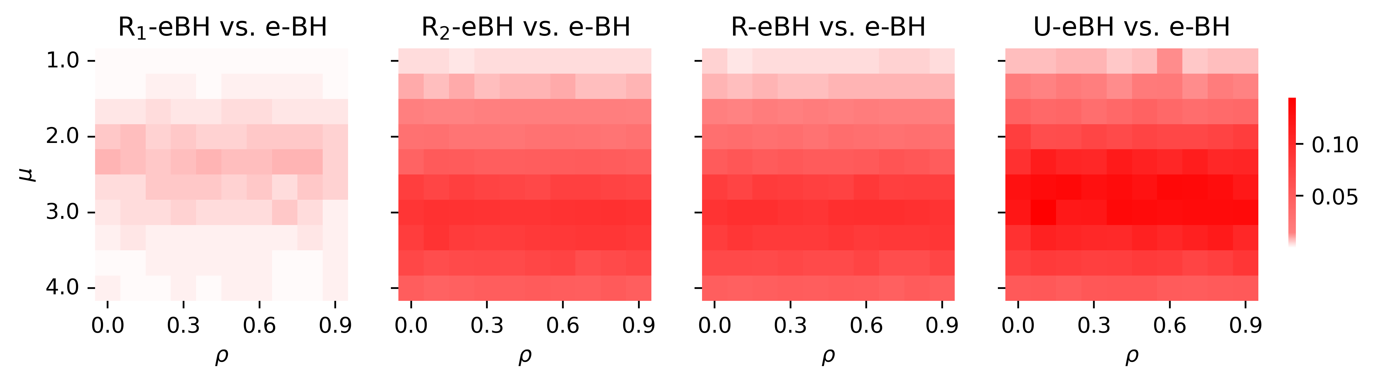
(a) Positive dependence: R₂-eBH, R-eBH, and U-eBH all have large power improvements over e-BH.

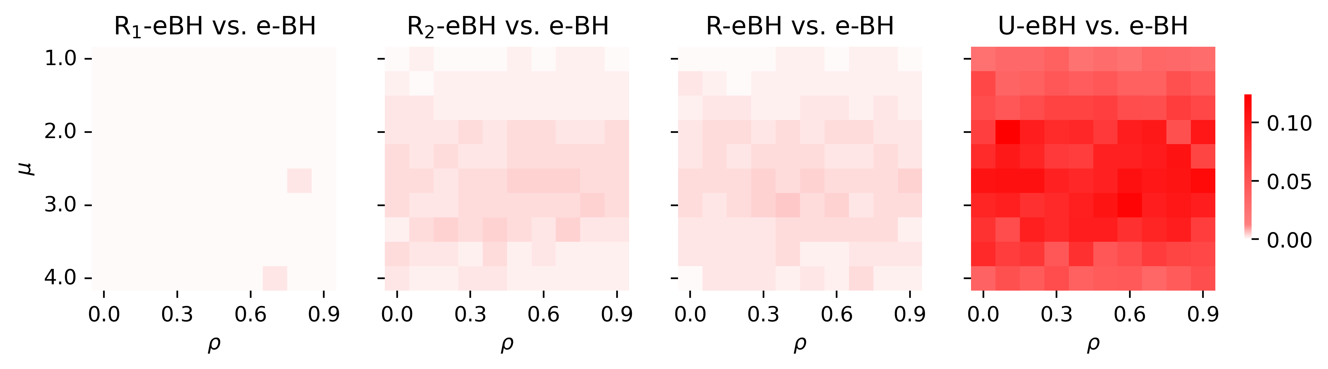
(b) Negative dependence: U-eBH is much more powerful than the other methods.

Figure 2: Heatmaps of the difference in power between randomized e-BH methods and e-BH. The hypotheses are one-sided tests of the mean of a standard Gaussian with covariance parameterized by $\rho$ (larger $\rho$ means larger covariance) and non-null means of $\mu$. As expected, U-eBH is the most powerful method across all settings, and randomized procedures uniformly improve over e-BH.

For each $i\in[K]$, where the null hypothesis is false, we let $\mu_{i}=\mu$, i.e., all non-null hypotheses have a single mean. Power is defined as the expected proportion of non-null hypotheses that are discovered, i.e., $\mathbb{E}[|\mathcal{D}-\mathcal{N}|/(K-|\mathcal{N}|)]$. We calculate the power averaged over 500 trials.

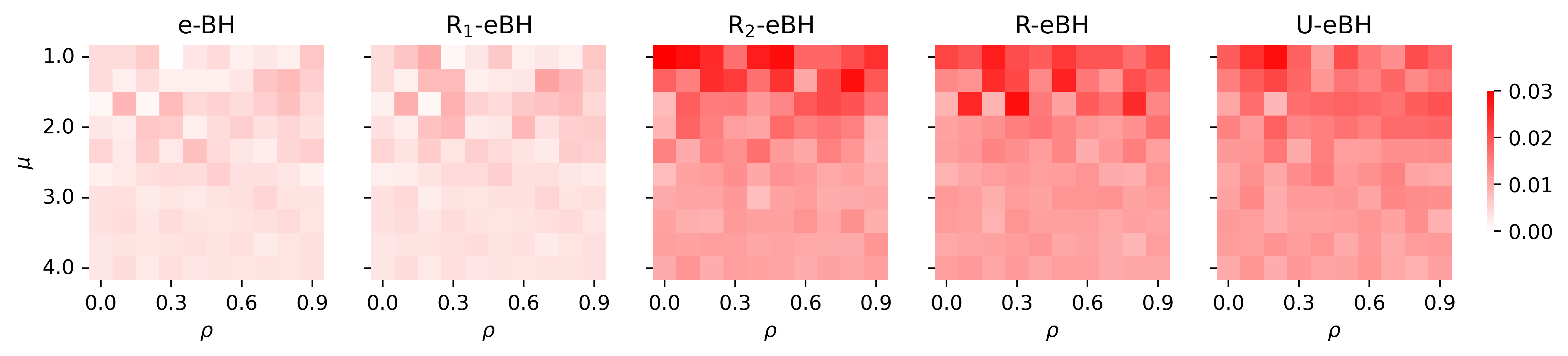
(a) Positive dependence: R₂-eBH, R-eBH, and U-eBH all have similar FDR.

(b) Negative dependence: U-eBH has much larger FDR across all settings.

Figure 3: Heatmaps of the achieved FDR of randomized e-BH methods and e-BH across different signal strength $\mu$ and correlation $\rho$. Note that all the FDR values are under the desired level of $\alpha=0.05$. Further, the randomized e-BH methods have higher realized FDR than e-BH (but still below $\alpha$), which is indicative of randomization providing tighter FDR control.

In Figure 2, we can see that R₁-eBH slightly increases power, while R₂-eBH provides a much larger improvement. Since the two types of rounding are complementary, R-eBH has the largest increase in power over e-BH. Further, we can see in Figure 3 that the FDR of all the methods is controlled to be below $\alpha=0.05$. Additional analysis of these results is in Appendix F.

(a) Positive dependence: U-BY has maximal power improvement when $\mu\in[2,3]$.

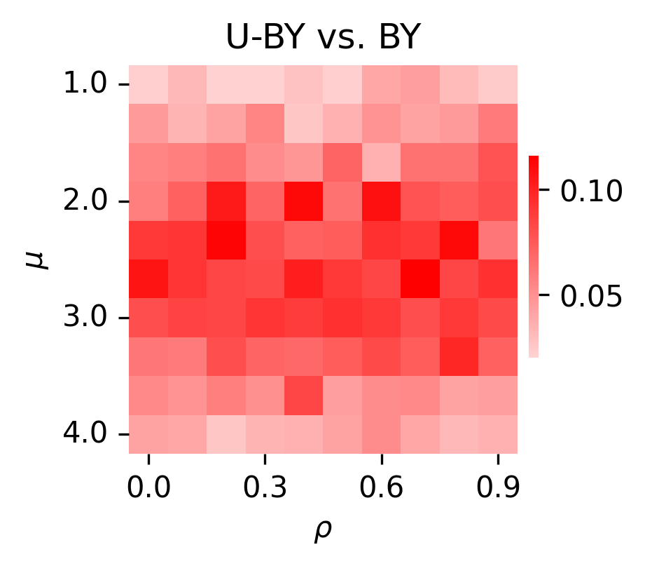
(b) Negative dependence: the power improvement of U-BY varies across $\rho$ and $\mu$.

Figure 4: Each pixel in the above heatmap captures the difference in power between U-BY and BY at the corresponding value of $\mu$ and $\rho$. The hypotheses are one-sided tests of the mean of a standard Gaussian that has covariance parameterized by $\rho$ (null means are 0 and non-null means are $\mu$). U-BY dominates the BY procedure across all $\rho$ and $\mu$.

In Figure 4, we compare the power of U-BY vs. BY. Similarly, U-BY uniformly dominates the BY procedure and shows a large amount of power improvement in most settings.

7 Conclusion

Stochastic rounding of e-values present a simple way of improving the power of multiple testing with e-values, and also procedures based on p-values that apriori appear to have nothing to do with e-values. While we have primarily discussed the use of stochastic rounding to improve the e-BH and BY procedures for FDR control, we also demonstrated that the idea works for other multiple testing procedures. In fact, one can also use these ideas to improve post-selection inference for confidence intervals with false coverage rate control (Benjamini and Yekutieli, 2005; Xu et al., 2022). Importantly, our randomized procedures always reject a superset of the rejection set produced by the original deterministic procedure. Among randomization techniques in the statistics literature (such as the bootstrap or sample splitting), this type of uniform improvement is rare, and moreover, implementing stochastic rounding in practice is quite simple.

One natural concern that may arise is whether the results of these randomized methods are reproducible. This concern can easily be addressed by using by using sources of randomness derived directly from the data itself (e.g., the order of the ranks in i.i.d. samples of data), as noted in Ramdas and Manole (2023, Section 10.6). Despite hesitations that may arise to use these randomized methods in practice, we believe our results are of significant theoretical and methodological interest. At the very least, our results should be quite surprising to the reader, since even the possibility that randomization can improve the power of deterministic procedures in multiple testing has not been previously considered, let alone constructively demonstrated.

Acknowledgments

We thank Ruodu Wang for his insightful comments and discussions including pointing out the application of stochastic rounding to admissible p-value merging in Appendix E.

Appendix A Proofs

A.1 Proof of Theorem 4

The FDR control is simply because we are running e-BH on e-values — to reproduce the proof from Wang and Ramdas (2022), we have that

$$\mathrm{FDR} =\sum\limits_{i\in\mathcal{N}}\mathbb{E}\left[\frac{\mathbf{1}\left\{S_{\widehat{\alpha}_{\ell(i)}}(X_{i})\geq K/(k^{*}_{\textnormal{U}}\alpha)\right\}}{k^{*}_{\textnormal{U}}\vee 1}\right]\leq\sum\limits_{i\in\mathcal{N}}\mathbb{E}\left[\frac{S_{\widehat{\alpha}_{\ell(i)},i}(X_{i})k^{*}_{\textnormal{U}}\alpha}{K(k^{*}_{\textnormal{U}}\vee 1)}\right]$$ (41)

$$=\frac{\alpha}{K}\sum\limits_{i\in\mathcal{N}}\mathbb{E}[S_{\widehat{\alpha}_{\ell(i)}}(X_{i})]\leq\alpha.$$ (42)

The first inequality is because $\mathbf{1}\left\{x\geq 1\right\}\leq x$ for any $x>0$, and the second inequality is because $S_{\widehat{\alpha}_{\ell(i)}}(X_{i})$ is an e-value for each $i\in[K]$.

Now, we want to show that U-eBH rejects all discoveries made by e-BH. To do so, we derive the following inequalities which hold for any $i\in\mathcal{D}_{\textnormal{eBH}}$:

$$\widehat{\alpha}_{\ell(i)}X_{i}\stackrel{{\scriptstyle\textnormal{(iv)}}}{{\mathstrut{\geq}}}\widehat{\alpha}_{\ell(i)}X_{[\ell(i)]}\stackrel{{\scriptstyle\textnormal{(v)}}}{{\mathstrut{\geq}}}\widehat{\alpha}_{k^{*}}X_{[k^{*}]}=\widehat{\alpha}^{*}X_{[k^{*}]}\stackrel{{\scriptstyle\textnormal{(vi)}}}{{\mathstrut{\geq}}}1,$$ (43)

where (43) is because $\mathbf{r}[i]\leq\ell(i)$ by the lower bound on the set $\ell(i)$ is the argmax over, (43) is by definition of $\ell(i)$ maximizing over a set that includes $k^{*}$ (since $X_{i}\geq X_{[k^{*}]}$ implies $\mathbf{r}[i]\geq k^{*}$), and (43) is by definition of e-BH. Further, we know $\widehat{\alpha}_{\ell(i)}\leq\widehat{\alpha}^{*}$ (i.e., $\ell(i)\leq k^{*}$) since $jX_{[j]}<K/\alpha\leq k^{*}X_{[k^{*}]}$ for all $j>k^{*}$ by definition of e-BH. Thus, we get the following inequalities:

$$X_{i}\geq 1/\widehat{\alpha}_{\ell(i)}\geq 1/\widehat{\alpha}^{*},$$ (44)

where the left inequality is by (43). Thus, $S_{\widehat{\alpha}_{\ell(i)}}(X_{i})\geq 1/\widehat{\alpha}^{*}$ for each $i\in\mathcal{D}_{\textnormal{eBH}}$, and we conclude all of $\mathcal{D}_{\textnormal{eBH}}$ is rejected.

The last thing we wish to show is $\mathbb{E}[k^{*}_{\textnormal{U}}]\geq\mathbb{E}[k^{*}_{2}]$. We observe the following follows by definition of stochastic rounding:

$$\mathbf{1}\left\{S_{\widehat{\alpha}_{\ell(i)}}(X_{i})\geq 1/\widehat{\alpha}_{\ell(i)}\right\}=\mathbf{1}\left\{U\leq\widehat{\alpha}_{\ell(i)}X_{i}\right\}.$$ (45)

Let $L\coloneqq\{\ell(i):i\in[K]\}$ be the set of levels that are rounded to. We define the following set of hypotheses for each $i\in L$:

$$\mathcal{D}_{i}\coloneqq\{j\in[K]:\widehat{\alpha}_{\ell(j)}\leq\widehat{\alpha}_{i}\}=\{j\in[K]:\mathbf{r}(j)\geq i\}.$$ (46)

By definition of $\ell$, the following properties are true:

$$|\mathcal{D}_{i}|=i\text{ for each }i\in L,\ignorespaces\ignorespaces$$

$$\mathcal{D}_{i}\subset\mathcal{D}_{i^{\prime}}\text{ for each }i,i^{\prime}\in L\text{ where }i<i^{\prime}.\ignorespaces\ignorespaces$$

Further, we can only reject numbers of hypotheses in $L$, i.e., $k^{*}_{\textnormal{U}}\in L$. This is because, for any $i\not\in L$, we know that $|\{j\in[K]:S_{\widehat{\alpha}_{\ell(j)}}(X_{j})\geq 1/\widehat{\alpha}_{i}\}|<i$ since for all $j\in[K]$ s.t. $X_{j}\geq X_{[i]}$, we have that $\ell(j)<i$. Hence, define $L(i)\coloneqq\min\{j\in L:j\geq i\}$, and we get the following relationship for any $i\geq k^{*}+1$:

$$\mathbf{1}\left\{k_{\textnormal{U}}^{*}\geq i\right\}=\mathbf{1}\left\{k^{*}_{\textnormal{U}}\geq L(i)\right\}.$$ (47)

Now, we derive the following property for each $i\in L$ where $i\geq k^{*}+1$:

$$\mathbf{1}\left\{k^{*}_{\textnormal{U}}\geq i\right\} =\mathbf{1}\left\{S_{\widehat{\alpha}_{\ell(j)}}(X_{j})\geq 1/\widehat{\alpha}_{\ell(j)}\text{ for all }j\in\mathcal{D}_{i}\right\}$$ (48)

$$=\mathbf{1}\left\{U\leq\widehat{\alpha}_{\ell(j)}X_{j}\text{ for all }j\in\mathcal{D}_{i}\right\}$$ (49)

$$=\mathbf{1}\left\{U\leq\widehat{\alpha}_{i}X_{[i]}\right\}.$$ (50)

The first line by (LABEL:eq:d-size) and (LABEL:eq:d-subset), and the observation that if $S_{\widehat{\alpha}_{\ell(j)}}(X_{j})=0$ for any $j\in\mathcal{D}_{i}$, there will be fewer than $i$ rejections. The equality in the second line is by (45), and the final equality is because—by definition of $\ell$—there exists $j\in\mathcal{D}_{i}$ s.t. $\ell(j)=i$ and $X_{j}=X_{[i]}$, and $\widehat{\alpha}_{\ell(j)}X_{j}\geq\widehat{\alpha}_{i}X_{[i]}$ for all $j\in\mathcal{D}_{i}$ by the definition of $\mathcal{D}_{i}$.

Thus, we have:

$$\mathbb{E}[k^{*}_{\textnormal{U}}\mid X_{1},\dots,X_{K}] =k^{*}+\sum\limits_{i=k^{*}+1}^{K}\mathbb{E}\left[\mathbf{1}\left\{k^{*}_{\textnormal{U}}\geq i\right\}\mid X_{1},\dots,X_{K}\right]$$ (51)

$$=k^{*}+\sum\limits_{i=k^{*}+1}^{K}\mathbb{P}\left(U\leq\widehat{\alpha}_{i}X_{[i]}\mid X_{1},\dots,X_{K}\right)$$ (52)

$$=k^{*}+\sum\limits_{i=k^{*}+1}^{K}\widehat{\alpha}_{i}X_{[i]}$$ (53)

$$\geq k^{*}+\sum\limits_{i=k^{*}+1}^{K}\widehat{\alpha}^{*}X_{[i]}$$ (54)

$$=k^{*}+\sum\limits_{i=k^{*}+1}^{K}\mathbb{P}\left(U_{i}\leq\widehat{\alpha}^{*}X_{[i]}\mid X_{1},\dots,X_{K}\right)$$ (55)

$$=\mathbb{E}[k^{*}_{2}\mid X_{1},\dots,X_{K}].$$ (56)

The second equality is by (50), and $U_{i}$ in the inequality are i.i.d. uniform random variables over $[0,1]$ for each $i\in[K]$.

A.2 Proof of Lemma 1

Define $R^{*}\coloneqq\inf\ \{s\in[R,\infty):P_{i}\leq c\beta(s)\}$. We note that

$$\mathbf{1}\left\{P\leq c\beta(R/U)\right\}=\mathbf{1}\left\{P\leq c\beta(R)\right\}+\mathbf{1}\left\{P>c\beta(R),U\leq R/R^{*}\right\}.$$ (57)

Hence, we simply need to prove that

$$\mathbb{E}\left[\frac{\mathbf{1}\left\{P\leq c\beta(R)\right\}+\mathbf{1}\left\{P>c\beta(R),U\leq R/R^{*}\right\}}{R}\right]\leq c.$$ (58)

The following proof repeatedly uses the fact that

$$1/z=\int_{0}^{\infty}\mathbf{1}\left\{r\geq z\right\}/z^{2}\ dr,\text{ for positive $z$}.$$ (59)

We begin with the following equalities:

$$\mathbb{E}\left[\frac{\mathbf{1}\left\{P\leq c\beta(R)\right\}+\mathbf{1}\left\{P>c\beta(R),U\leq R/R^{*}\right\}}{R}\right]$$ (60)

$$=\mathbb{E}\left[\int\limits_{0}^{\infty}\frac{\mathbf{1}\left\{r\geq R,P\leq c\beta(R)\right\}}{r^{2}}\ dr+\frac{\mathbf{1}\left\{P>c\beta(R),U\leq R/R^{*}\right\}}{R}\right]$$ (61)

$$=\mathbb{E}\left[\int\limits_{0}^{\infty}\frac{\mathbf{1}\left\{r\geq R,P\leq c\beta(R),P\leq c\beta(r)\right\}}{r^{2}}\ dr\right]+\mathbb{E}\left[\frac{\mathbf{1}\left\{P>c\beta(R),U\leq R/R^{*}\right\}}{R}\right].$$ (62)

Now, we can get the following equalities for the right summand:

$$\mathbb{E}\left[\frac{\mathbf{1}\left\{P>c\beta(R),U\leq R/R^{*}\right\}}{R}\right]$$ (63)

$$=\mathbb{E}\left[\frac{\mathbf{1}\left\{P>c\beta(R)\right\}\mathbb{E}[\mathbf{1}\left\{U\leq R/R^{*}\right\}\mid R,P]}{R}\right]$$ (64)

$$\stackrel{{\scriptstyle\textnormal{(vii)}}}{{\mathstrut{=}}}\mathbb{E}\left[\frac{\mathbf{1}\left\{P>c\beta(R)\right\}}{R^{*}}\right]$$ (65)

$$=\mathbb{E}\left[\mathbf{1}\left\{P>c\beta(R)\right\}\int\limits_{0}^{\infty}\frac{\mathbf{1}\left\{r\geq R^{*}\right\}}{r^{2}}dr\right]$$ (66)

$$\stackrel{{\scriptstyle\textnormal{(viii)}}}{{\mathstrut{=}}}\mathbb{E}\left[\mathbf{1}\left\{P>c\beta(R)\right\}\int\limits_{0}^{\infty}\frac{\mathbf{1}\left\{r\geq R,P\leq c\beta(r)\right\}}{r^{2}}\ dr\right].$$ (67)

The equality in (65) is by the independence and the uniform distribution of $U$. The equality in (67) is by definition of $R^{*}$, i.e., $r\geq R^{*}$ if and only if $P\leq c\beta(r)$ and $r\geq R$. Now, we can combine (58), (62) and (67) to derive the following:

$$\mathbb{E}\left[\frac{\mathbf{1}\left\{P\leq c\beta(R/U)\right\}}{R}\right]$$ (68)

$$=\mathbb{E}\left[\int\limits_{0}^{\infty}\frac{\mathbf{1}\left\{r\geq R,P\leq c\beta(R),P\leq c\beta(r)\right\}}{r^{2}}\ dr\right]+\mathbb{E}\left[\int\limits_{0}^{\infty}\frac{\mathbf{1}\left\{r\geq R,P>c\beta(R),P\leq c\beta(r)\right\}}{r^{2}}\ dr\right]$$ (69)

$$=\mathbb{E}\left[\int\limits_{0}^{\infty}\frac{\mathbf{1}\left\{r\geq R,P\leq c\beta(r)\right\}}{r^{2}}\ dr\right]=\int\limits_{0}^{\infty}\frac{\mathbb{P}\left(r\geq R,P\leq c\beta(r)\right)}{r^{2}}\ dr$$ (70)

$$\stackrel{{\scriptstyle\textnormal{(ix)}}}{{\mathstrut{\leq}}}\int\limits_{0}^{\infty}\frac{\mathbb{P}\left(P\leq c\beta(r)\right)}{r^{2}}\ dr\stackrel{{\scriptstyle\textnormal{(x)}}}{{\mathstrut{\leq}}}c\int\limits_{0}^{\infty}\frac{\beta(r)}{r^{2}}\ dr$$ (71)

$$=c\int\limits_{0}^{\infty}x\int\limits_{0}^{\infty}\frac{\mathbf{1}\left\{r\geq x\right\}}{r^{2}}\ dr\ d\nu(x)=c\int_{0}^{\infty}d\nu(x)=c.$$ (72)

We get (71) by taking the probability of a superset, and (71) is by superuniformity of $P$. Consequently, we have proven our lemma.

A.3 Proof of Proposition 4

Let $k^{*}_{\text{BH}}$ represent the number of rejections made BH. First, we note that both the BH view and the U-eBH formulation will reject the hypotheses corresponding to the $k^{*}_{\text{BH}}$ and $k^{*}_{\textnormal{U}}$ largest e-values. The number of rejections made by BH are as follows:

$$k^{*}_{\text{BH}}=\max\left\{k\geq 1:\frac{U}{X_{[k]}}\leq\frac{\alpha k}{K}\right\}=\max\left\{k\geq 1:U\leq\frac{\alpha kX_{[k]}}{K}\right\}$$ (73)

Now, we simply want to show that

$$k^{*}_{\textnormal{U}}=\ell^{*}\coloneqq\max\left\{\ell(i):U\leq\alpha X_{i}\ell(i)/K,i\in[K]\right\}=k^{*}_{\text{BH}}.$$ (74)

We will first argue the left equality is true. Stochastic rounding rejects the $i$th hypothesis if and only if $U\leq\alpha X_{i}\ell(i)/K$ by expanding the definition of $\widehat{\alpha}_{\ell(i)}$ and applying (17). $U\leq\alpha X_{i}\ell(i)/K$ if and only if $\ell(i)\leq\ell^{*}$, and exactly $\ell^{*}$ hypotheses satisfy that.

The right equality is true because if $k^{*}_{\text{BH}}>\ell^{*}$, then the definition of $\ell$ is violated, as $k^{*}_{\text{BH}}X_{[k^{*}_{\text{BH}}]}>\ell(i)X_{[\ell(i)]}$ for some $i$ where $\ell(i)\leq\ell^{*}$. If $\ell^{*}>k^{*}_{\text{BH}}$, this violates the definition $k^{*}_{\text{BH}}$, as $\ell^{*}>k^{*}_{\text{BH}}$ and $U\leq\alpha kX_{[\ell^{*}]}/K$. Thus, we have shown (74) is true, and our desired result follows.

A.4 Proof of Theorem 6

Since $\beta$ is monotonic, $\beta(k^{*}_{\beta})\leq\beta(k^{*}_{\beta}/U_{i})$ for every $i\in[K]$, so $k^{*}_{\beta}\leq k^{*}_{\beta,\textnormal{U}}$. Now, define the following quantities:

$$m(i)\coloneqq\max\{u\in[0,1]:P_{(i)}\leq\alpha\beta(i/u)/K\},\qquad t(i)\coloneqq\underset{j\geq\mathbf{r}(i)}{\text{argmax}}\ m(j).$$ (75)

where $\mathbf{r}(i)\coloneqq\sum_{j\in[K]}\mathbf{1}\left\{P_{j}\leq P_{i}\right\}$ refers to the rank of $P_{i}$ in ascending order of p-values. We claim that

$$\mathbf{1}\left\{P_{i}\leq\alpha\beta(k^{*}_{\beta,\textnormal{U}}/U)/K\right\}=\mathbf{1}\left\{P_{i}\leq\alpha\beta(t(i)/U)/K\right\}.$$ (76)

If the right side equals 1, $k^{*}_{\beta,\textnormal{U}}\geq t(i)\geq\mathbf{r}(i)$ by construction, so the left side equals 1. On the other hand, if the right side equals 0, then we know $U>m(j)$ for all $j\geq\mathbf{r}(i)$. This means that at most $\mathbf{r}(i)-1$ hypotheses are rejected, and $\mathbf{r}(i)-1<t(i)$, so the left side is also 0.

We can now look at the FDR of the $\beta$-reshaped U-BY procedure.

$$\mathrm{FDR} =\sum\limits_{i\in\mathcal{N}}\mathbb{E}\left[\frac{\mathbf{1}\left\{P_{i}\leq\alpha\beta(k^{*}_{\beta,\textnormal{U}}/U)/K\right\}}{k^{*}_{\beta,\textnormal{U}}\vee 1}\right]$$ (77)

$$\stackrel{{\scriptstyle\textnormal{(xi)}}}{{\mathstrut{\leq}}}\sum\limits_{i\in\mathcal{N}}\mathbb{E}\left[\frac{\mathbf{1}\left\{P_{i}\leq\alpha\beta(t(i)/U)/K\right\}}{t(i)}\right]\stackrel{{\scriptstyle\textnormal{(xii)}}}{{\mathstrut{\leq}}}\sum\limits_{i\in\mathcal{N}}\frac{\alpha}{K}\leq\alpha.$$ (78)

We know (78) is true by (76) and $t(i)\leq k^{*}_{\beta,\textnormal{U}}$ whenever the $i$th hypothesis is rejected. Inequality (78) is by Lemma 1. Thus, we have proven FDR control for any reshaping function $\beta$.

Appendix B Conditions for strict improvement by stochastic rounding

Our theorems in the paper guarantee that the randomized e-BH procedures do no worse than the original e-BH in power. We will now formulate conditions where the power of these randomized version are strictly more powerful.

B.1 R₁-eBH 

For R₁-eBH, we introduce two natural conditions.

Condition 1.

$(X_{1},\dots,X_{K})$ are not supported solely over $\mathcal{K}$.

This condition is necessary, since if $(X_{1},\dots,X_{K})$ lay on $\mathcal{K}$ exactly, then there would be no rounding possible, as rounding precisely exploits the gap between the support of each e-value and $\mathcal{K}$.

Condition 2.

$(X_{1},\dots,X_{K})$ is supported on a set such that for all $(x_{1},\dots,x_{K})$ in this set, e-BH applied to $(x_{1}^{+},\dots,x_{K}^{+})$ results in more discoveries.

This is non-degeneracy condition, i.e., there do exists realizations of the e-values where if every e-value $X_{i}$ was rounded up to $X_{i}^{+}$, e-BH would actually make more discoveries.

Then, we have that R₁-eBH  is more powerful.

Proposition 6.

If Condition 1 and Condition 2 both hold, then R₁-eBH  is strictly more power than e-BH, i.e., $k^{*}_{1}>k^{*}$ with positive probability.

B.2 R₂-eBH  R-eBH, and U-eBH

For R₂-eBH, R-eBH, and U-eBH, we can relax our requirements to a condition that is weaker than Condition 2.

Condition 3.

$\mathbb{P}\left(\exists i\in[K]:0<X_{i}<\widehat{\alpha}^{*}\right)>0$, i.e., there is positive probability that e-BH does not reject all hypotheses and at least one e-value, corresponding to an hypothesis that is not rejected by e-BH, is nonzero.

This condition is nearly always satisfied in practice, since it only excludes the trivial situations where e-values that do not meet threshold of rejection are zero or every hypothesis has been rejected. Hence we note that R₂-eBH and U-eBH have greater power over e-BH in most scenarios.

Proposition 7.

For any arbitrarily dependent e-values $(X_{1},\dots,X_{K})$, R₂-eBH, R-eBH, and U-eBH all reject a strict superset of the hypotheses rejected by e-BH, i.e., $\mathcal{D}_{\textnormal{eBH}}\subset\mathcal{D}_{2},\mathcal{D}_{\textnormal{R}},\mathcal{D}_{\textnormal{U}}$ with nonzero probability when Condition 3 is satisfied.

B.3 U-BY

We can also show a similar result for the U-BY procedure by translating Condition 3 into the language of p-values.

Condition 4.

For p-values $(P_{1},\dots,P_{K})$, $\mathbb{P}\left(\exists i\in[K]:\widehat{\alpha}_{k^{*}_{\mathrm{BY}}}/\ell_{K}<P_{i}\leq\alpha/\ell_{K}\right)>0$, that is, there is a positive probability that BY does not reject all hypotheses and at least one p-value, corresponding to a hypothesis that is not rejected by BY, that is at most $\alpha/\ell_{K}$.

Proposition 8.

For any arbitrarily dependent p-values $(P_{1},\dots,P_{K})$, the U-BY procedure rejects a strict superset of the hypotheses rejected by BY, i.e., $\mathcal{D}_{\text{BY}}\subset\mathcal{D}_{U-\text{BY}}$ with nonzero probability, when Condition 4 is satisfied.

Appendix C U-BY when the FDR control is sharp

One might wonder what the behavior of U-BY is when applied to the p-value distribution constructed by Guo and Bhaskara Rao (2008), on which BY applied at level $\alpha$ has an FDR of exactly $\alpha$. We will show that in this situation U-BY has a behavior that is identical to BY, and also has an FDR of exactly $\alpha$.

Let $K_{0}\in[K]$ be the number of null hypotheses — let the first $K_{0}$ hypotheses be true nulls (i.e., $\mathcal{N}=[K_{0}]$ is the set of true nulls), and the remaining hypotheses be non-nulls (i.e, $\{K_{0}+1,\dots,K\}=[K]\setminus[K_{0}]$). For a specific level $\alpha\in[0,1]$, Guo and Bhaskara Rao (2008) begin their construction by sampling $N\in[K+1]$ according to the following distribution:

$$\mathbb{P}\left(N=n\right)=\begin{cases}\alpha K_{0}/(nK\ell_{K})&\text{ for }n\in[K_{0}]\\ \alpha/(K\ell_{K})&\text{ for }n\in\{K_{0}+1,\dots,K\}\\ 1-\alpha\left(1+(\ell_{K_{0}}-1)K_{0}\right)/(K\ell_{K})&\text{ for }n=K+1\end{cases}.$$ (79)

Let $U_{0}$ and $U_{1}$ be independent, uniform random variables in $[0,1]$.

1. If $N\leq K$, draw $I_{0}\subseteq[K_{0}]$ uniformly randomly from the subsets of $[K_{0}]$ that are of size $N\wedge K_{0}$. If $N>K_{0}$, additionally draw $I_{1}\subseteq[K]\setminus[K_{0}]$ uniformly randomly from subsets of $[K]\setminus[K_{0}]$ that are of size $N-K_{0}$ — otherwise let $I_{1}=\emptyset$. Let $I\coloneqq I_{0}\cup I_{1}$. Now, we define our p-values as follows:

   $$P_{i}=\begin{cases}\alpha(N-1+U_{0})/(K\ell_{K})&\text{ for }i\in I\\ \alpha/\ell_{K}+(1-\alpha/\ell_{K})U_{1}&\text{ for }i\not\in I\end{cases}.$$ (80)

2. Otherwise, if $N=K+1$, the p-values are generated as follows:

   $$P_{i}=\begin{cases}\alpha/\ell_{K}+(1-\alpha/\ell_{K})U_{0}\text{ for }i\in[K_{0}]\\ 1\text{ for }i\in[K]\setminus[K_{0}]\end{cases}..$$ (81)

Fact 1 (Theorem 5.1 (iii) of Guo and Bhaskara Rao (2008)).

The BY procedure, when applied to the aforementioned p-value distribution characterized by (80) and (81), has an FDR of exactly $\alpha(K+K_{0}(\ell_{K_{0}}-1))/(K\ell_{K})$. Note that, when $K_{0}=K$, the FDR of BY is exactly $\alpha$.

We note that in this setting, BY always rejects all hypotheses corresponding to p-values less than $\alpha/\ell_{K}$. Hence, U-BY cannot improve upon BY, as U-BY never rejects any hypotheses with p-values above $\alpha/\ell_{K}$. Thus, BY and U-BY should have exactly the same FDR in this setting. We verify through simulations in Figure 5, where we set $\alpha=0.05$, $K=10^{5}$, vary $\pi_{0}\coloneqq K_{0}/K$ in $[0,1]$, and plot the FDR calculated from simulations against the FDR derived in Fact 1. Clearly, BY and U-BY have identical empirical FDR that matches closely to what Fact 1 indicates.

Figure 5: Plot of proportion of nulls, $\pi_{0}$, vs. the FDR (estimated through simulations) of different FDR controlling procedures applied at level $\alpha=0.05$ (denoted by the dashed grey line) in the setting described in Guo and Bhaskara Rao (2008). The bands surrounding each line are 95% CIs for the FDR that arise from Monte Carlo error. The dashed black line indicates the exact FDR of BY derived theoretically by Guo and Bhaskara Rao (2008). BH clearly does not ensure $\mathrm{FDR}\leq\alpha$. Both BY and U-BY have identical estimates and closely match the theoretical FDR.

Appendix D Generalization of stochastic rounding

One might wish to generalize stochastic rounding (to the nearest points in $\mathcal{G}$) to instead take a probability distribution over values in $\mathcal{G}$ that are at greater than or equal to $x^{+}$. For e-BH, the simplest such generalization would be to assign a uniform probability to all potential e-BH rejection levels greater than the input $x$. Let $r=x-x_{-}$, and define $j^{+}=K/(\alpha x^{+})$ . Then, we would define $S^{\mathrm{uni}}_{\mathcal{G}}(X)$ a follows:

$$S^{\mathrm{uni}}_{\mathcal{G}}(x)=\begin{cases}\frac{K}{\alpha j}&\text{ with probability }\frac{\alpha r}{KH_{j^{+}}}\\ x_{-}&\text{ with probability }1-\frac{\alpha rj^{+}}{KH_{j^{+}}}.\end{cases}$$ (82)

Another way of generalizing the stochastic rounding is to have equal “expectation” assigned to each potential e-BH rejection level. We would have $p_{j}\propto j$, where $p_{j}$ is the probability of outputting $K/(\alpha j)$ for some $j\geq j^{+}$.

$$S^{\mathrm{eq}}_{\mathcal{G}}(x)=\begin{cases}\frac{K}{\alpha j}&\text{ with probability }\frac{\alpha jr}{Kj^{+}}\text{ for }j\in[j^{+}]\\ x_{-}&\text{ with probability }1-\frac{\alpha r(j^{+}+1)}{2K}.\end{cases}$$ (83)

More generally, we know that we can consider $\mathcal{G}^{+}(x)\coloneqq\{y\in\mathcal{G}:y\geq x\}$, i.e., the set of values in the grid greater than $x$. Let $F_{x}$ be the c.d.f. of a distribution over $\mathcal{G}^{+}(x)$ for each $x$ that satisfies

$$p^{+}(x)\cdot\int\limits_{y\in\mathcal{G}^{+}(x)}y\ dF_{x}(y)+(1-p^{+}(x))x_{-}=x,$$ (84)

where $p^{+}(x)\in[0,1]$ is the probability $X$ is made larger by stochastic rounding. Let $S^{+}_{\mathcal{G}}(X)$ be our generalized stochastically rounded e-value i.e.,

$$S^{+}_{\mathcal{G}}(x)\coloneqq\begin{cases}Y&\text{ where }Y\sim F_{x}\text{ ind. of }X\text{ with probability }p^{+}(x)\\ x_{-}&\text{ with probability }(1-p^{+}(x)).\end{cases}$$ (85)

Proposition 9.

If $X$ is an e-value, then $\mathbb{E}[S^{+}_{\mathcal{G}}(X)]$ is an e-value. Further, $\mathbb{E}[X]=\mathbb{E}[S^{+}_{\mathcal{G}}(X)]$.

The above proposition follows from the definition of $S^{+}_{\mathcal{G}}$, and (84). We also note that in the multiple testing setting we can allow the $Y$ that is sampled to be dependent on all the e-values $(X_{1},\dots,X_{K})$ while still having a conditional distribution with expectation $x$. This allows us to adaptively choose the rounding distribution $F_{x}$ for all $x\in[0,\infty)$ based on the randomized e-values results so far, if randomization is done sequentially over the e-values.

Joint generalized rounding (the J-eBH procedure)

We can extend this generalized rounding idea to allow for joint distribution across the rounded e-values. In essence, our rounding scheme would be, given some input e-values $(X_{1},\dots,X_{K})$, the rounded e-values $(S_{\mathcal{G}_{1}}^{+}(X_{1}),\dots,S_{\mathcal{G}_{K}}^{+}(X_{K}))$ satisfy the following:

$$\mathbb{E}[S_{\mathcal{G}_{i}}^{+}(X_{i})\mid X_{i}]=X_{i}.$$ (86)

In the context of joint generalized rounding procedures for e-BH, a desideratum is the following:

$$i\not\in\mathcal{D}\text{ if and only if }S_{\mathcal{G}_{i}}^{+}(X_{i})=0\text{ for all }i\in[K].$$ (87)

This means the rounding procedure is “efficient” in some sense, since the e-value wastes no probability mass on values that are insufficiently large to be rejected. We note that the U-eBH and R₂-eBH both satisfy (87). For the e-BH procedure, we can push a generalized joint rounding scheme even further, and requires that it satisfies the following:

$$i\in\mathcal{D}\text{ and }X_{i}<1/\widehat{\alpha}^{*}\text{ if and only if }S_{\mathcal{G}_{i}}^{+}(X_{i})=1/\widehat{\alpha}_{|\mathcal{D}|}.$$ (88)

Note that neither U-eBH nor R₂-eBH satisfy (88) — the rounding procedures in both cases round e-values to values that are larger than necessary to be rejected. Hence, we can characterize a class of generalized rounding procedures that satisfy (88).

We define a singular grid for all e-values: $\mathcal{G}_{i}=\mathcal{K}_{k^{*}}\coloneqq\{1/\widehat{\alpha}_{j}:j>k^{*},j\in[K]\}$ for each $i\in[K]$. Since $1/\widehat{\alpha}^{*}$ is larger than the max element of $\mathcal{K}_{k^{*}}$, all $X_{i}$ that are rejected by e-BH do not change after rounding. Now, we wish to define a joint distribution $F_{(X_{1},\dots,X_{K})}$ in the following fashion: let $\mathcal{J}_{(X_{1},\dots,X_{K})}$ be our rounding distribution over $\mathbf{J}\in\{0,1\}^{K}$ where the $\mathbf{J}_{i}=1$ for each $i\in\mathcal{D}_{\textnormal{eBH}}$. We draw a sample $\mathbf{J}$, and define the rounded e-value as follows:

$$S_{\mathcal{K}_{k^{*}}}^{+}(X_{i})=(X_{i}\cdot\mathbf{1}\left\{X_{i}\geq 1/\widehat{\alpha}^{*}\right\})\vee\frac{\mathbf{J}_{i}}{\widehat{\alpha}_{||\mathbf{J}||_{0}}},$$ (89)

where $||\cdot||_{0}$ is the number of nonzero entries or zeroth norm. Note that under this sampling scheme, (88) is satisfied, since $||\mathbf{J}||_{0}=|\mathcal{D}|$. We refer this as the J-eBH procedure, and denote its discovery set as $\mathcal{D}_{\textnormal{J}}$ with cardinality $k^{*}_{\textnormal{J}}$.

One such choice of $\mathcal{J}_{(X_{1},\dots,X_{K})}$ is the one induced by defining $\mathbf{J}_{i}$ as follows:

$$\mathbf{J}_{i}=\mathbf{1}\left\{U_{i}\leq X_{i}\widehat{\alpha}_{U}^{*}\right\},$$ (90)

where $1/\widehat{\alpha}_{U}^{*}$ is the rejection threshold of BH when applied to $(U_{1}/X_{1},\dots,U_{K}/X_{K})$, where $(U_{1},\dots,U_{K})$ are uniform random variables which are joinly independent and independent of $(X_{1},\dots,X_{K})$.

Proposition 10.

If $(X_{1},\dots,X_{K})$ are e-values, then $(S_{\mathcal{K}_{k^{*}}}(X_{1}),\dots,S_{\mathcal{K}_{k^{*}}}(X_{K}))$ are e-values, where the rounding distribution is characterized by (90).

Proof.

For brevity, we use the notation $\mathbf{X}\coloneqq(X_{1},\dots,X_{K})$. We will show ${\mathbb{E}[S_{\mathcal{K}_{k^{*}}}(X_{i})\mid\mathbf{X}]=X_{i}}$ for each $i\in[K]$. This is trivially true for $i\in\mathcal{D}_{\textnormal{eBH}}$. We can note the following for each $k>k^{*}$ and $i\not\in\mathcal{D}_{\textnormal{eBH}}$:

$$\mathbb{P}\left(S_{\mathcal{K}_{k^{*}}}(X_{i})=1/\widehat{\alpha}_{k}\mid\mathbf{X}\right)$$ (91)

$$=\mathbb{P}\left(||\mathbf{J}||_{0}=k,\mathbf{J}_{i}=1\mid\mathbf{X}\right)$$ (92)

$$=\sum\limits_{\mathbf{A}:||\mathbf{A}||_{0}=k,\mathbf{A}_{i}=1}\mathbb{P}\left(\forall j\in[K]:\mathbf{1}\left\{U_{j}\leq X_{j}\widehat{\alpha}_{j}\right\}=\mathbf{A}_{j}\mid\mathbf{X}\right)$$ (93)

$$=\mathbb{P}\left(U_{i}\leq X_{i}\widehat{\alpha}_{i}\mid\mathbf{X}\right)\sum\limits_{\mathbf{A}:||\mathbf{A}||_{0}=k,\mathbf{A}_{i}=1}\mathbb{P}\left(\forall j\in[K]\setminus\{i\}:\mathbf{A}_{j}=\mathbf{1}\left\{U_{j}\leq X_{j}\widehat{\alpha}_{j}\right\}\mid\mathbf{X}\right),$$ (94)

where the last equality is by independence of $U_{i}$.

Now, we note the following, where we assume $X_{1},\dots,X_{K}$ are fixed quantities for brevity of notation:

$$\mathbb{E}[S_{\mathcal{K}_{k^{*}}}(X_{i})\mid\mathbf{X}]$$ (95)

$$=\sum\limits_{j=k^{*}+1}^{K}\frac{\mathbb{P}\left(S_{\mathcal{K}_{k^{*}}}(X_{i})=1/\widehat{\alpha}_{j}\mid\mathbf{X}\right)}{\widehat{\alpha}_{j}}$$ (96)

$$=\sum\limits_{j=k^{*}+1}^{K}\sum\limits_{\mathbf{A}:||\mathbf{A}||_{0}=j,\mathbf{A}_{i}=1}\mathbb{P}\left(\forall k\in[K]\setminus\{i\}:\mathbf{A}_{i}=\mathbf{1}\left\{U_{i}\leq X_{i}\widehat{\alpha}_{i}\right\}\mid\mathbf{X}\right)$$ (97)

$$\leq 1$$ (98)

where the last equality is by (94) and the last inequality is because the summations are over disjoint events. Thus, we have shown our desired result.

∎

Given the above proposition, we can now assert the FDR of J-eBH is controlled.

Theorem 9.

For any arbitrarily dependent e-values, $(X_{1},\dots,X_{K})$, the J-eBH procedure controls $\mathrm{FDR}\leq\alpha$. Further, J-eBH rejects all hypotheses that e-BH rejects, i.e., $\mathcal{D}_{\textnormal{eBH}}\subseteq\mathcal{D}_{\textnormal{J}}$.

Further, one can see that as a result of its definition in (90), J-eBH with rounding distribution specified by (90) is equivalent to applying BH to $(U_{1}/X_{1},\dots,U_{K}/X_{K})$. Of course, any $\mathcal{J}$ that can satisfy (86) is sufficient to derive a valid J-eBH procedure, and we leave exploration of what the best choice is to future work.

Simulations

In the same setting as Section 6, we compare J-eBH and U-eBH. The difference in their power is shown in Figure 6. Interestingly, neither method dominates the other. U-eBH is more powerful when there is negative dependence or $\mu$ is small and positive dependence. On the other hand, J-eBH is more powerful when there is positive dependence and $\mu$ is large. This suggests one avenue for future work is to identify whether there is a single optimal joint generalized rounding scheme, and if not, in what situations are different schemes optimal.

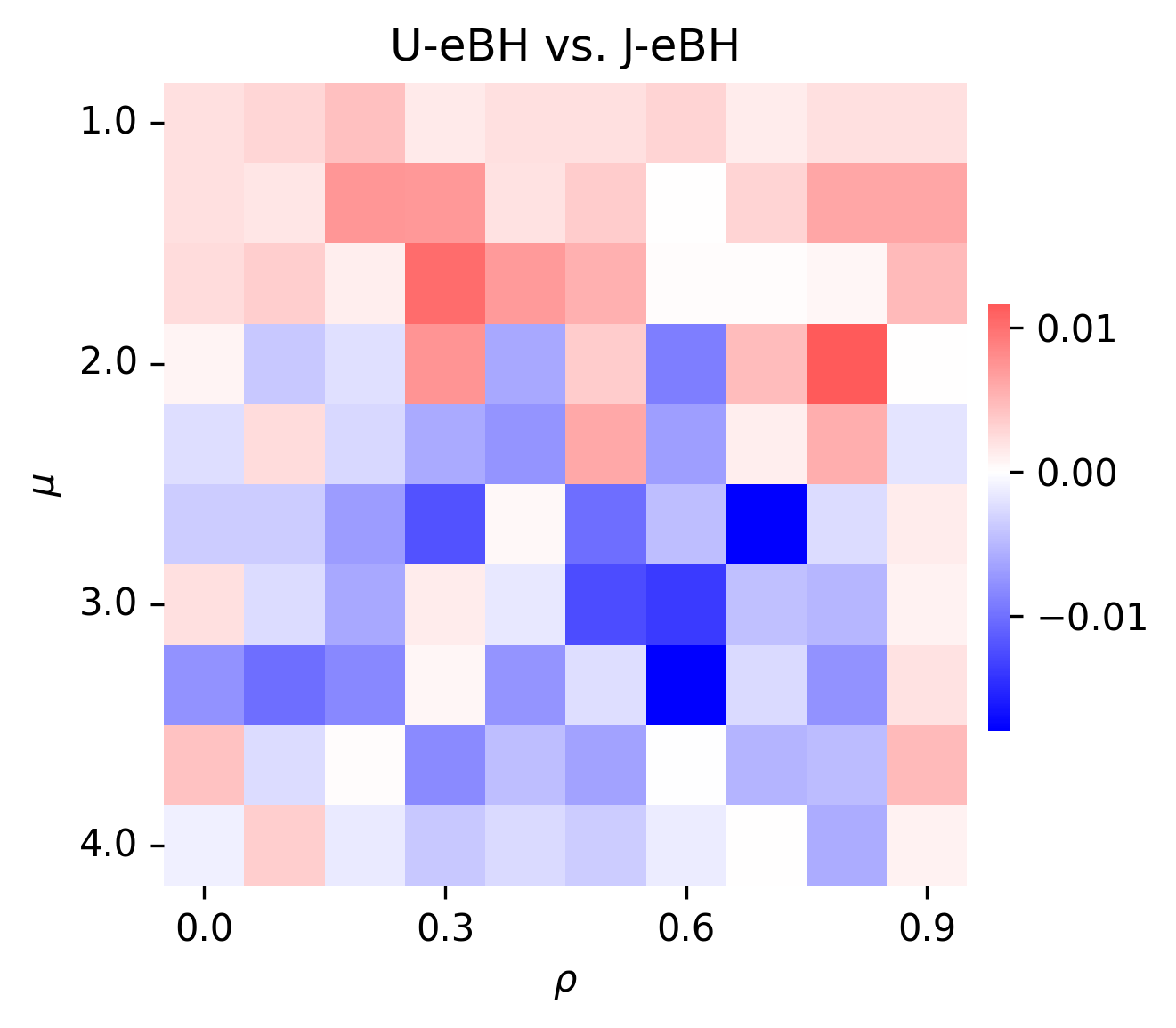
(a) Positive dependence: U-eBH is more powerful when $\mu$ is smaller, while J-eBH is more powerful when $\mu$ is larger.

(b) Negative dependence: U-eBH dominates J-eBH across the board.

Figure 6: Heatmaps of the difference in power of using U-eBH vs J-eBH, i.e., single $U$ vs. a independent $U_{i}$, across different values of $\mu$ and $\rho$ in the same simulation setting as described in Section 6. U-eBH is more powerful when the dependence is negative, or when the signal is smaller under positive dependence, while J-eBH is more powerful when the dependence is positive and $\mu$ is small.

Appendix E Randomizing admissible p-merging functions

We can extend our results from Section 4 concerning the Hommel p-merging function to randomize admissible p-merging functions in general. Formally, we define a p-merging function $F:[0,\infty)^{K}\rightarrow[0,\infty)$ to be a function where $F(\mathbf{P})$ is a p-value if $\mathbf{P}=(P_{1},\dots,P_{K})$ is a vector of $K$ arbitrarily dependent p-values. Note that p-values are usually restricted to the domain $[0,1]$, but the definition of p-merging functions relaxes the domain to $[0,\infty)$ for simplicity. We also call $F$ homogeneous if $F(\lambda\mathbf{p})=\lambda F(\mathbf{p})$ for any $\lambda\in(0,1]$ and $\mathbf{p}\in[0,\infty)^{K}$. The class of homogeneous p-merging functions includes the analog of the Bonferroni correction, methods introduced by Hommel (1983) and Rüger (1978) based on order statistics, and functions that use p-value averages devised by Vovk and Wang (2020).

Vovk et al. (2022) prove that any admissible homogeneous p-merging function has a dual form that is formulated in terms of calibrators. We will leverage this dual form to apply our randomization techniques and produce randomized p-merging functions that are never greater than the p-values produced by the unaltered p-merging function. The key representation result that we use is the following:

Fact 2 (Vovk et al. 2022; Theorem 5.1).

Let $R_{\alpha}(F)\coloneqq\{\mathbf{p}\in[0,\infty)^{K}:F(\mathbf{p})\leq\alpha\}$. For any admissible homogeneous p-merging function $F$, there exist $(\lambda_{1},\dots,\lambda_{K})\in\Delta^{K}$ ($\Delta^{K}$ is the simplex on $K$ dimensions) and admissible calibrators $f_{1},\dots,f_{K}$ such that:

$$X(\mathbf{p}) \coloneqq\sum\limits_{i=1}^{K}\lambda_{i}f_{i}(p_{i})\text{ and }$$ (99)

$$R_{\alpha}(F) =\left\{\alpha\cdot\mathbf{p}:\mathbf{p}\in[0,\infty)^{K},X(\mathbf{p})\geq 1\right\}\text{ for each }\alpha\in(0,1),$$ (100)

where $p_{i}$ is the $i$th component of $\mathbf{p}$. Conversely, for any $(\lambda_{1},\dots,\lambda_{K})\in\Delta^{K}$ and calibrators $(f_{1},\dots,f_{K})$, (100) determines a homogeneous p-merging function.

Note that $X(\mathbf{P})$ is an e-value in the definition above. Hence, we can define a randomized p-merging function by stochastically rounding $X(\mathbf{P})$. Let $\widetilde{F}$ be the randomized version of the p-merging function $F$, where $F$ can be represented by (100). We can define the rejection region of $\widetilde{F}$ in the following fashion:

$$R_{\alpha}(\widetilde{F}) \coloneqq\left\{\alpha\cdot\mathbf{p}\in[0,\infty)^{K}:S_{1}(X(\mathbf{p}))\geq 1\right\}$$ (101)

$$=\left\{\alpha\cdot\mathbf{p}\in[0,\infty)^{K}:X(\mathbf{p})\geq U\right\}\text{ for each }\alpha\in(0,1),$$ (102)

where $U$ is a uniform random variable.

Theorem 10.

$\widetilde{F}$ with the randomized rejection region defined in (102) is a bona-fide p-merging function. Further $\widetilde{F}(\mathbf{p})\leq F(\mathbf{p})$ for any $\mathbf{p}\in[0,\infty)^{K}$.

Proof.

First, we want to show the validity of this randomized p-merging function by proving the following:

$$\mathbb{P}\left(\mathbf{P}\in R_{\alpha}(\widetilde{F})\right) =\mathbb{P}\left(S_{1}(X(\mathbf{P}/\alpha))\geq 1\right)\leq\alpha.$$ (103)

To show this, we use the same argument as Vovk et al. (2022), and we can make the following derivation:

$$\mathbb{E}[X(\mathbf{P}/\alpha)] =\sum\limits_{i=1}^{K}\lambda_{i}\mathbb{E}[f_{i}(P_{i}/\alpha)]\leq\sum\limits_{i=1}^{K}\lambda_{i}\int\limits_{0}^{1}f_{i}(x/\alpha)\ dx=\alpha\sum\limits_{i=1}^{K}\lambda_{i}\int\limits_{0}^{1/\alpha}f_{i}(x)\ dx=\alpha.$$ (104)

The first inequality is because each $f_{i}$ is a calibrator. The last equality is because $f_{i}(x)=0$ for $x>1$ since $f_{i}$ is a calibrator, and $\sum_{i\in[K]}\lambda_{i}=1$ by definition. Consequently, $\mathbb{E}[S_{1}(X(\mathbf{P}/\alpha))]\leq\alpha$ as a result of stochastic rounding, i.e., Proposition 2. By Markov’s inequality, we know that (103) is true.

We know also know the following chain of implications by definition of $F$:

$$F(\mathbf{p})\leq\alpha\Leftrightarrow\sum\limits_{i=1}^{K}\lambda_{i}f_{i}(p_{i}/\alpha)\geq 1\Rightarrow\sum\limits_{i=1}^{K}\lambda_{i}f_{i}(p_{i}/\alpha)\geq U\Leftrightarrow\widetilde{F}(\mathbf{p})\leq\alpha.$$ (105)

The implication in the above chain is simply because $1\geq U$ is always true. Hence, we have shown our desired result. ∎

Theorem 10 now allows us to define a large family or randomized p-merging functions that improve over admissible deterministic p-merging functions. An example of such a p-merging function from Vovk et al. (2022) is the grid harmonic merging function which dominates the Hommel function and the domination is strict when $K\geq 4$. It is defined using the formulation in (100) and the following calibrator:

$$f^{\textnormal{GH}}(x)\coloneqq\frac{K\mathbf{1}\left\{\ell_{K}x\leq 1\right\}}{\lceil K\ell_{K}x\rceil}.$$ (106)

Consequently, the grid harmonic merging function, $F^{\textnormal{GH}}$, has a rejection region that is defined as follows:

$$R_{\alpha}(F^{\textnormal{GH}})\coloneqq\left\{\alpha\cdot\mathbf{p}:\sum\limits_{i=1}^{K}\frac{K\mathbf{1}\left\{\ell_{K}p_{i}\geq 1\right\}}{\lceil K\ell_{K}x\rceil}\geq 1\right\}.$$ (107)

Applying our randomization approach, we can define $\widetilde{F}^{\textnormal{GH}}$ as follows:

$$R_{\alpha}(\widetilde{F}^{\textnormal{GH}})\coloneqq\left\{\alpha\cdot\mathbf{p}:\sum\limits_{i=1}^{K}\frac{K\mathbf{1}\left\{\ell_{K}p_{i}\leq 1\right\}}{\lceil K\ell_{K}x\rceil}\geq U\right\}.$$ (108)

Appendix F Additional simulations

We performed some additional simulations to probe the differences between methods more deeply. We can see the improvement of using R-eBH over each of the stochastic rounding approaches individually in Figure 7. Notably, R₂-eBH is not uniformly dominated by R-eBH in all simulation settings, but it is beaten in the majority of them, particularly when the signal strength, $\mu$, is smaller.

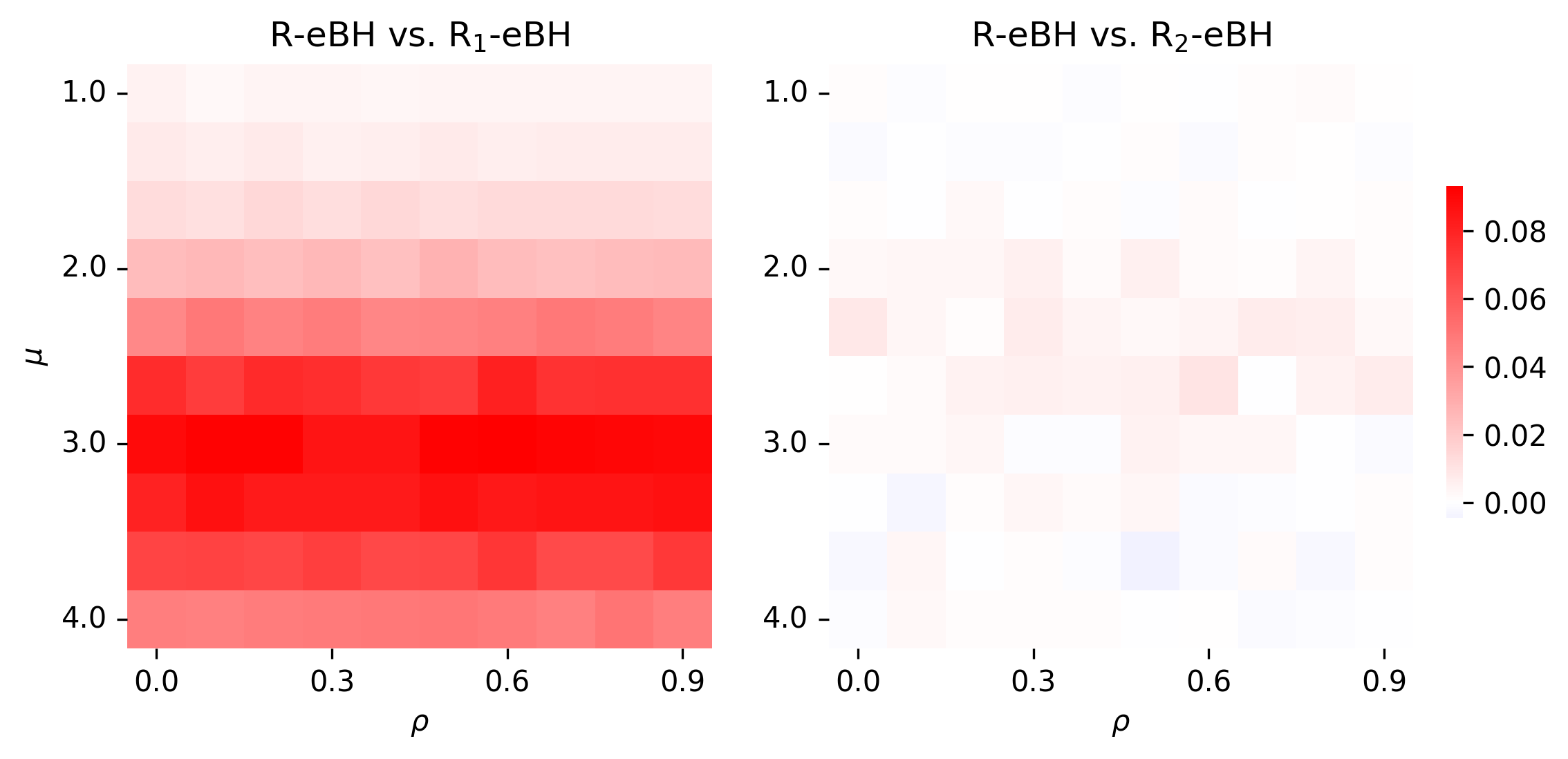
(a) Positive dependence: R-eBH performs much better than R₁-eBH and slightly better than R₂-eBH when $\mu$ is small.

(b) Negative dependence: R-eBH performs better than R₁-eBH, but neither R-eBH nor R₂-eBH dominate the other.

Figure 7: Heatmap of the difference in power of using R-eBH over either R₁-eBH  or R₂-eBHacross different values of $\mu$ and $\rho$ in the same simulation setting as described in Section 6. R-eBH clearly performs better than R₁-eBH. Compared to R₂-eBH, R-eBH performs only better in some settings.

Another comparison to consider is the relationship between the e-BH procedure and using the BY procedure with $U_{i}/X_{i}$. We can see in Figure 8 that BY applied to $U_{i}/X_{i}$ has much lower power, and therefore is beaten even by baseline e-BH.

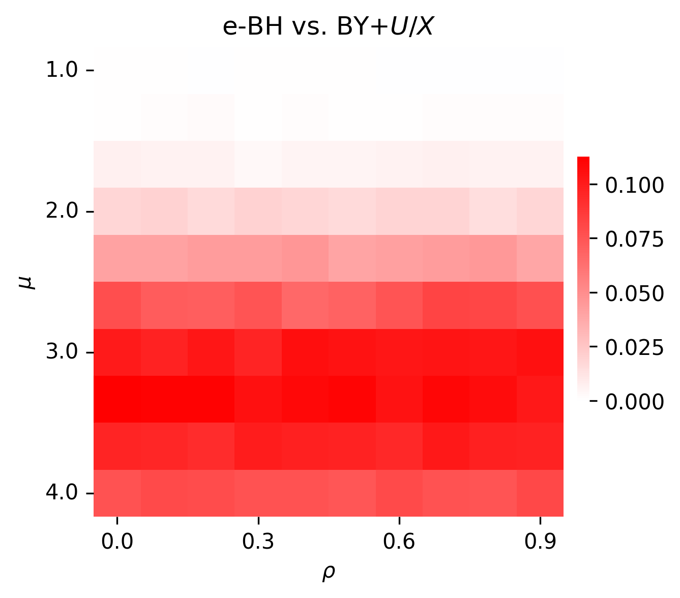
(a) Positive dependence: e-BH dominates applying BY to $U/X_{i}$ across all $\mu$ and $\rho$.

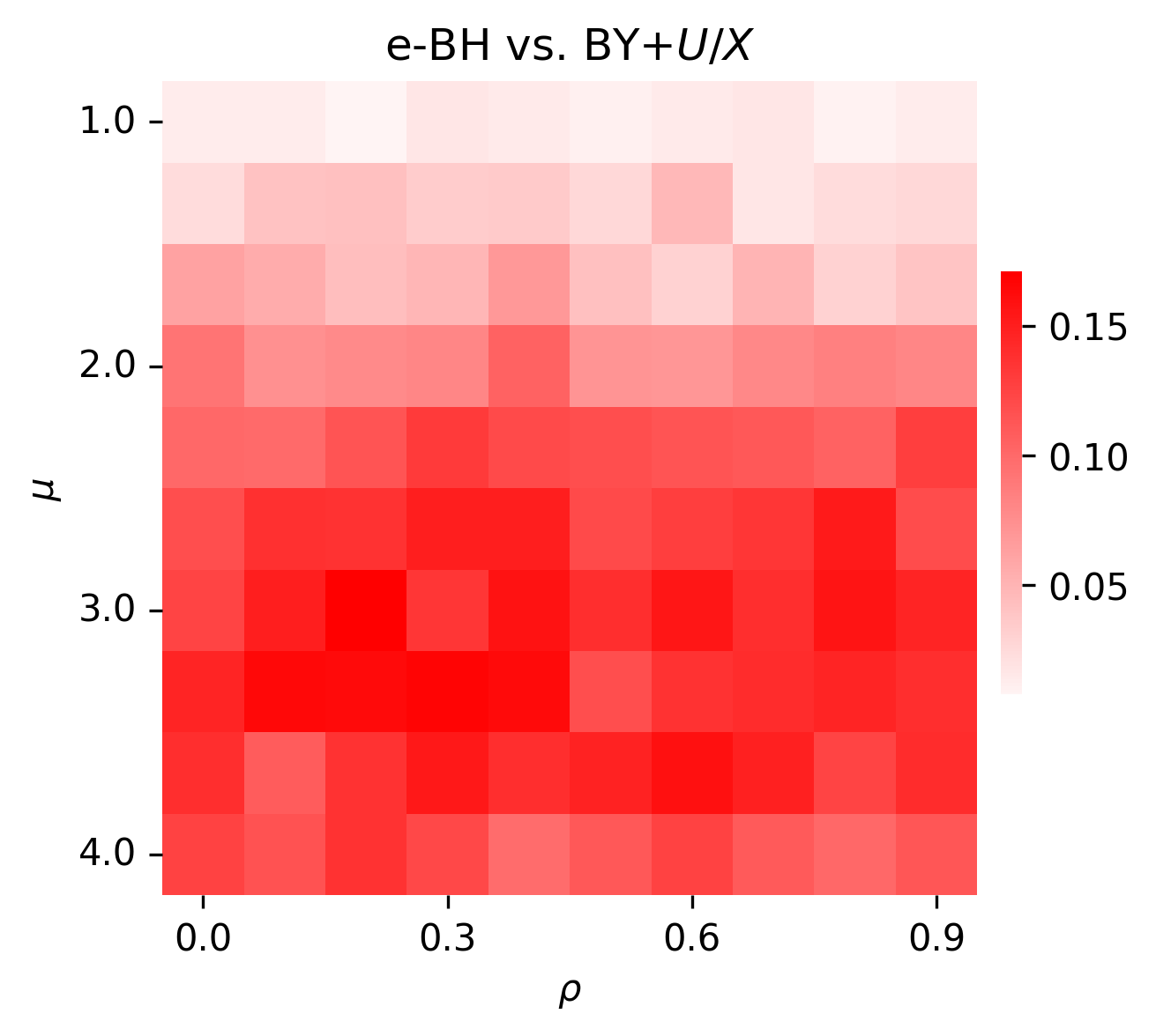
(b) Negative dependence: e-BH also dominates BY with $U/X_{i}$ for all $\mu$ and $\rho$ here too.

Figure 8: Heatmap of the difference in power of using e-BH over applying BY to $U_{i}/X_{i}$ across different values of $\mu$ and $\rho$ in the same simulation setting as described in Section 6.

We also compare how the use of a single $U_{i}=U$ for all uniform random variables instead of independent $U_{i}$ affects the performance of R₂-eBH and R-eBH in Figure 9. There is no particular relationship between which one is better or worse, so it does not seem like selecting one vs. the other makes a significant difference in the procedure.

(a) Positive dependence: independent $U_{i}$ seem to be better on average, particularly for R-eBH.

(b) Negative dependence: Single $U$ seems to be better on average, particularly for R-eBH.

Figure 9: Heatmaps of the difference in power of using independent $U_{i}$ vs. a single $U$ (i.e., $U_{i}=U$ for each $i\in[K]$) across different values of $\mu$ and $\rho$ (as described in Section 6).

References

- Benjamini and Hochberg (1995) Y. Benjamini and Y. Hochberg. Controlling the False Discovery Rate: A Practical and Powerful Approach to Multiple Testing. Journal of the Royal Statistical Society. Series B (Methodological), 57(1):289–300, 1995.
- Benjamini and Yekutieli (2001) Y. Benjamini and D. Yekutieli. The control of the false discovery rate in multiple testing under dependency. The Annals of Statistics, 29(4):1165–1188, 2001.
- Benjamini and Yekutieli (2005) Y. Benjamini and D. Yekutieli. False Discovery Rate–Adjusted Multiple Confidence Intervals for Selected Parameters. Journal of the American Statistical Association, 100(469):71–81, 2005.
- Blanchard and Roquain (2008) G. Blanchard and E. Roquain. Two simple sufficient conditions for FDR control. Electronic Journal of Statistics, 2:963–992, 2008.
- Dunn et al. (2022) R. Dunn, A. Gangrade, L. Wasserman, and A. Ramdas. Universal Inference Meets Random Projections: A Scalable Test for Log-concavity. arXiv:2111.09254, 2022.
- Gangrade et al. (2023) A. Gangrade, A. Rinaldo, and A. Ramdas. A Sequential Test for Log-Concavity. arXiv:2301.03542, 2023.
- Grünwald et al. (2023) P. Grünwald, R. de Heide, and W. Koolen. Safe Testing. Journal of the Royal Statistical Society: Series B (forthcoming), 2023.