Blackout Diffusion: Generative Diffusion Models in Discrete-State Spaces

Abstract

Typical generative diffusion models rely on a Gaussian diffusion process for training the backward transformations, which can then be used to generate samples from Gaussian noise. However, real world data often takes place in discrete-state spaces, including many scientific applications. Here, we develop a theoretical formulation for arbitrary discrete-state Markov processes in the forward diffusion process using exact (as opposed to variational) analysis. We relate the theory to the existing continuous-state Gaussian diffusion as well as other approaches to discrete diffusion, and identify the corresponding reverse-time stochastic process and score function in the continuous-time setting, and the reverse-time mapping in the discrete-time setting. As an example of this framework, we introduce “Blackout Diffusion”, which learns to produce samples from an empty image instead of from noise. Numerical experiments on the CIFAR-10, Binarized MNIST, and CelebA datasets confirm the feasibility of our approach. Generalizing from specific (Gaussian) forward processes to discrete-state processes without a variational approximation sheds light on how to interpret diffusion models, which we discuss.

1 Introduction

Diffusion processes have been recently utilized to construct Diffusion Models, a class of generative models in deep learning (Sohl-Dickstein et al., 2015; Ho et al., 2020; Song et al., 2021d). These frameworks consist of a set of trainable transformations (implemented as deep neural networks) that sequentially process a prescribed distribution (the prior, usually a high-dimensional isotropic Gaussian) to the data distribution. To train the networks, samples drawn from the data distribution are transformed by a stochastic process, which goes forward in time, and which has the prior as a stationary (final) distribution. Realizations from the forward diffusion process are used to train transformations that approximate the reverse-time process. In generative inference, samples are drawn from the prior, and the trained network is used to transform them into samples of the learned data distribution.

Diffusion Models have been used for many applications, including image (Sohl-Dickstein et al., 2015; Ho et al., 2020; Nichol & Dhariwal, 2021; Song & Ermon, 2019, 2020; Song et al., 2021d, b), audio (Kong et al., 2021), video (Höppe et al., 2022; Ho et al., 2022), and language (Gong et al., 2022). Most works follow the original formulation (Sohl-Dickstein et al., 2015; Ho et al., 2020), utilizing Gaussian diffusion on continuous domains. However, there are wide-ranging data domains which are not continuous in nature, and applying quantization and de-quantization for treating these data may not be ideal. For example, single-molecule and single-cell gene expressions (Munsky et al., 2015; Pichon et al., 2018) study systems with very small counts, in which discrete effects are qualitatively relevant to system behavior. As another example, phase-separated fluid problems occur in many applications pertaining to industrial and earth sciences, where each region of space is occupied categorically, that is, by exactly one of several fluid types (Li et al., 2016). Graph structures are pervasive and machine learning on these structures is an area of tremendous recent growth (Zhou et al., 2020), for example being the dominant representation for molecular structure, which is of relevance to chemistry (Gilmer et al., 2017), drug discovery (Wieder et al., 2020; Smith et al., 2018), and biophysics (Jiang et al., 2021). In bioinformatics, both DNA and protein sequences are codes consisting of discrete values (Ingraham et al., 2019).

Some prior works have investigated diffusion modeling beyond the Gaussian paradigm. For example, Bansal et al. (2022) challenged the notion that noise is required by showing that deterministic degradation (e.g. blurring) applied to images, constructing a deterministic alternative, and discarding the stochastic theory entirely. Despite the abundance of potential applications, few theoretical formulations diffusion modeling of arbitrary discrete-state systems have been proposed. Sohl-Dickstein et al. (2015) explores a particular form of binomial diffusion kernels as a discrete-time diffusion. Ye et al. (2022) proposed leveraging the exit distribution of first-passage processes to achieve discrete-state generative modeling. Termed as the First Hitting Diffusion Models (FHDM), the underlying process is still a continuous-state Gaussian (Itô) diffusion, but FHDM can sample discrete-state distributions without ad hoc quantization and dequantization. Most relevant to our work include (1) Multinomial Diffusion (Hoogeboom et al., 2021), which invoked a specific discrete Markovian process (the multinomial process) and solved for the corresponding reverse process analytically, (2) Austin et al. (2021) created Masked Diffusion using a discrete-state Markov chain as the forward diffusion which transforms samples to a unique “masked state”, and (3) the recent work by Campbell et al. (2022) described a theoretical framework for continuous-time discrete-state Generative Diffusion Modeling. Importantly, the theories developed in both Austin et al. (2021); Campbell et al. (2022) take a variational inference approach to constructing the loss function, and Campbell et al. (2022) achieves a continuous-time formulation by taking a limit of this approach. An exact (i.e. non-variational) analysis has not been seen in the existing literature.

Addressing diffusion for arbitrary discrete-state processes requires answering several questions. For example, is there a discrete-state formula corresponding to the Brownian bridge used in Ho et al. (2020) for learning the reverse-time mappings, and more broadly, is diffusion modeling only possible when there are closed-form solutions for reverse-time mapping? What is the Stein score function (Song & Ermon, 2019, 2020; Song et al., 2021d, b) for learning the reverse-time process? Our contribution is to answer these questions and put forth a general and exact theoretical framework for constructing Diffusion Models in discrete-state spaces for an arbitrary Markov process, which can be either discrete-time or continuous-time in nature. Our core contribution is a prescription for the generator of the reverse-time stochastic process, forming the discrete analog to Anderson (1982) for Itô Stochastic Differential Equations (SDEs).

We then examine explicitly a specific case, the pure-death process, which corresponds physically to radioactive decay. In this case, the prior consists of a single point—a completely black image, similar to Mask Diffusion (Austin et al., 2021). Based on this characteristic, we call this approach Blackout Diffusion. We emphasize that our process is different from Mask Diffusion (Austin et al., 2021), although both processes (almost-surely) converge to a singular state as $t\rightarrow\infty$. We show that Blackout Diffusion can learn and generate the CIFAR-10, CelebA, and Binarized MNIST datasets without interpreting the data as continuous at any stage. Additionally, we consider how discrete-state models answer two additional conceptual questions regarding generative Diffusion Models: (1) Do the forward and reverse stochastic processes have to correspond to noisifying and denoising processes? (2) Is it natural to consider the prescribed prior as a latent-space representation, as can be done for normalizing flows (Rezende & Mohamed, 2015) and variational autoencoders (Kingma & Welling, 2014)?

The rest of the paper is structured as follows. Section 2 presents the construction of discrete-space forward, backward and reverse processes, loss functions and score functions, and the relationship to Gaussian diffusion. For the rest of the article, we choose a particular Markov model, Blackout Diffusion defined in Sec. 2.5, presenting results in Sec. 3 and questions raised in Sec. 4.

2 Method

There are several key components to tractable Diffusion Models. First, one must be able to sample the forward stochastic process efficiently for generating the training data. Secondly, one needs to analytically prescribe summary statistics for training the backwards transformations; learning from individual samples would be computationally prohibitive. Existing generative Diffusion Models (Sohl-Dickstein et al., 2015; Ho et al., 2020; Nichol & Dhariwal, 2021; Song & Ermon, 2019, 2020; Song et al., 2021d, b) use a particular Gaussian diffusion process which is applied independently in the dimension of the data, e.g. in each color channel of each pixel in an image, for which the theoretical formulation is complete. For discrete-time implementations (Sohl-Dickstein et al., 2015; Nichol & Dhariwal, 2021), the forward solution is analytically tractable, and the summary statistics—the conditional mean and variance of the reverse-time mapping—can be obtained via the Brownian bridge technique (Revuz & Yor, 1994). For continuous-time implementations (Song & Ermon, 2019, 2020; Song et al., 2021d, b), the forward solution is also tractable, and the summary statistics (the drift and diffusion of SDE) for the reverse-time process were provided by Anderson (1982).

In this section, we present the theoretical formulation for generative modeling using discrete-state Markov processes. Detailed derivations can be found in the Appendices. We present the forward and backward Kolmogorov equations (Sec. 2.2), and reverse-time processes (Sec. 2.3) for discrete-space diffusion modeling. We further elaborate (Sec.2.4) on the continuum limit of discrete-state systems, providing the connection to continuous-state systems, and describing the discrete-state score functions. The loss functions (Sec. 2.6) and sample generation (Sec. 2.7) procedures are also provided.

2.1 Notations

State space. We consider an $N$-dimensional state space $\Omega^{N}$, where each dimension of the data lives in a finite discrete-state space $\Omega$, and each state is labeled and ordered by $\left\{0\ldots M\right\}$. For example, in CIFAR-10, $N=32\times 32\times 3$ and $\Omega=\left\{0,1,\ldots M=255\right\}$. A state in this space, a high-dimensional random variable, is denoted by $\mathbf{X}\in\Omega^{N}$. For most of the derivations, it suffices to consider a single dimension (one color channel of a particular pixel) which will be denoted by $X\in\Omega$. We will use the lower-case symbols (e.g., $m$, $n$, $o$) to denote the dummy state variable. We will use the subscript to denote the time parameter of the random process: For discrete-time systems, the random process is denoted as $\mathbf{X}_{k}$, $k\in\mathbb{Z}_{\geq 0}$, and continuous-time random process is denoted as $\mathbf{X}_{t}$, $t\geq 0$.

Probability distributions. We use $p$ to denote joint or conditional probabilities. In addition, a shorthand notation will be employed, for example with times $s,\,t\geq 0$,

$$p_{(m,t)}:={} \mathbb{P}\left\{X_{t}=m\right\},$$ (1a)

$$p_{(n,t)|(m,s)}:={} \mathbb{P}\left\{X_{t}=n|X_{s}=m\right\},$$ (1b)

$$p_{(m,s),(n,t)|(o,0)}:={} \mathbb{P}\left\{X_{s}=m,X_{t}=n|X_{0}=o\right\}.$$ (1c)

2.2 Forward and Backward equations

The forward process is described by the Chapman–Kolmogorov equations (Kolmogorov, 1931; van Kampen, 2007; Gardiner, 2009). We will consider a one-dimensional Markov process applied independently to each of the dimensions of the joint state $\mathbf{X}$. In the continuous-time setting, the forward equation can be written as a Master Equation (van Kampen, 2007; Gardiner, 2009; Weber & Frey, 2017):

$$\frac{\text{d}}{\text{d}t}p_{(m,t)|(o,0)}=\sum_{m^{\prime}}L^{\dagger}_{mm^{\prime}}p_{(m^{\prime},t)|(o,0)},$$ (2)

where $L$ is the generator of the continuous-time and discrete-state stochastic process and $L^{\dagger}$ is the adjoint operator of $L$.

We first explain our results for a subset of Markov processes where the states are only allowed to transition between neighboring states, so that the generator in Eq. (2) have a tri-diagonal structure. For this subset of processes, it is convenient to use the step operators (van Kampen, 2007) to reformulate the forward equation (2). The step operators $\mathcal{E}_{\pm}$ are defined by $\mathcal{E}_{\pm}f(m)\triangleq f(m\pm 1)$ for any test function $f$. Employing the Einstein summation convention for the $\pm$ signs $\sigma\in\left\{+,-\right\}$, the forward equation (2) can be expressed by

$$\frac{\text{d}}{\text{d}t}p_{(m,t)|(o,0)}=\left(\mathcal{E}_{\sigma}^{\dagger}-1\right)\left[\nu_{\sigma}(m)\,p_{(m,t)|(o,0)}\right]$$ (3)

where $\nu_{\sigma}(m)$ is the transition rate from state $m$ to $m+\sigma\cdot 1$.

The backward equation for the continuous-time process (3) is the Kolmogorov backward equation (Kolmogorov, 1931; van Kampen, 2007; Gardiner, 2009) for the transition probabilities from state $m$ at an earlier time $s\geq 0$ to state at $n$ at a later time $t$:

$$-\frac{\text{d}}{\text{d}s}p_{(n,t)|(m,s)}=\nu_{\sigma}(m)\left(\mathcal{E}_{\sigma}-1\right)p_{(n,t)|(m,s)}.$$ (4)

2.3 Reverse-time process

Here we prescribe the reverse-time stochastic process, analogous to the prescription of Anderson (1982) which is applied for Gaussian diffusion. Formally, the reverse-time process describes how conditional probability $p_{(m,s)|(n,T),(o,0)}$, $0\leq s\leq T$, evolves reversely in time, which is necessary for designing the likelihood or loss function and for generation, thereby laying the foundation for Diffusion Model learning and inference. Here, we present the results, and leave the detailed derivations in Appendix A.

For the continuous-time Markov process (3), the reverse-time evolutionary equation for any time $0\leq s\leq t$ reads

$$-\frac{\text{d}}{\text{d}s}{} p_{(m,s)|(n,t),(o,0)}=$$ (5)

$$\left(\mathcal{E}_{\sigma}-1\right)\left[\nu_{\sigma}\left(m_{\sigma}^{\prime}\right)\frac{p_{(m^{\prime}_{\sigma},s)|(o,0)}}{p_{(m,s)|(o,0)}}p_{(m,s)|(n,t),(o,0)}\right].$$

Note that the reverse-time process is an explicitly time-dependent Markov process, whose transition rates depend on the forward solution $p_{(m,s)|(n,0)}$. This is analogous to the fact that the drift and diffusion of the reverse-time Gaussian diffusion processes depend on the forward solution (Anderson, 1982). Note also that a state $m$ later in time can transit to a state $m^{\prime}$ at an early time only if there exists a transition $m^{\prime}\rightarrow m$ defined in the forward process (see Remark 1 in Appendix A). These expressions, derived from formal operator algebra, can be understood intuitively as a conditional Bayes formula (see Appendix A).

While Eqs. (3)-(5) are specific to tri-diagonal transitions, all of these results generalize to arbitrary transition matrices, as shown in Appendix B, by writing the transition matrix as a sum over banded processes and exploiting linearity. We also remark that the theory applies to arbitrary discrete-state spaces. The state space does not have to be ordered, although it is ordered in our application of image dataset below. Finally, as illustrated in Appendix A, there exists a corresponding theory for generic discrete-time and discrete-time stochastic processes.

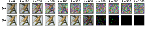
Figure 1: The forward process of (a) Gaussian diffusion and (b) Blackout Diffusion applied on an image, sampled at discrete time $k$. The colormap is adjusted per-image to better visualize the noisy signal of Blackout Diffusion at large times. Fig. 5 shows images with unadjusted colormap.

2.4 Relationship to Gaussian diffusion

To shed light on the connection between our discrete-state diffusion formulas and Gaussian diffusion, we use Kramers–Moyal expansion (van Kampen, 2007; Gardiner, 2009; Weber & Frey, 2017), a standard asymptotic analysis to study the limiting behavior in a state space with large number discrete states ($M\gg 1$) densely distributed in $\Omega$. Appendix C presents the formal expansion, showing that both the forward and reversal discrete-state processes asymptotically converge to the standard (multiplicative) Gaussian diffusion in this limit. Importantly, the asymptotic expansion of the discrete-state reversal process is consistent with the reversal process (by Anderson (1982)) of the asymptotically expanded forward process.

Performing the continuous limit also allows the identification of the discrete-state score function $s_{\mathrm{dis,\sigma}}$:

$$s_{\text{dis},\sigma}\left(m,s\right)\propto\nu_{\sigma}\left(m^{\prime}_{\sigma}\right)\frac{p_{(m^{\prime}_{\sigma},s)|(o,0)}-p_{(m,s)|(o,0)}}{p_{(m,s)|(o,0)}},$$ (6)

which is an analog to the Stein score function, the key learning target for score-based generative models (Song & Ermon, 2019, 2020; Song et al., 2021d, b). Interestingly, there is a transformation to learn for each type of transition event into state $m$, rather than simply a transformation for each feature in the data. (see discussion in Appendices C and G).

2.5 Blackout Diffusion

Here, we choose a simple Markov process to illustrate the utility of the proposed discrete-state formulation. The process is adequate for the digital images, whose state space $\Omega=\left\{0\ldots 255\right\}$ is discrete and naturally ordered. One of the simplest processes of this class is the pure-death process, such that the only event is the transition $m\in\Omega$ to $m-1$ with a transition rate $\gamma m$:

$$m\xrightarrow{\gamma m}m-1.$$ (7)

The pure-death process is a mathematical model for constant, independent decay, such as in radioactivity. For digital image data, it can be interpreted as such: Each unit intensity of a specific pixel and color channel decays from $1$ to $0$ with a rate $\gamma$. This process is a homogenous stochastic process, that is, the transition rate is constant in time. We can arbitrarily set the timescale such that $\gamma=1$. With Eq. (2), the transition matrix can be defined by a banded $L^{\dagger}_{mm^{\prime}}=m^{\prime}\left(\delta_{m,m^{\prime}-1}-\delta_{m,m^{\prime}}\right)$, where $\delta$ is the Kronecker delta. Note that the pure-death process is distinct from Mask Diffusion (Austin et al., 2021), which has one-step transition from any state to the absorbing state, per pixel and per channel. For pure-death process, a state $n$ requires $n$ transition events before it reaches the absorbing state $0$, per pixel and per channel. The two processes are very similar on binary data, only differing in that Masked Diffusion is non-homogenous process (i.e., the transition rate is time-dependent). With the representation Eq. (3), we have the negative transition $\nu_{-}(m)=m$ and the positive transition $\nu_{+}(m)=0$, $m\in\Omega$. It is elementary to derive the solution of the forward process as a binomial distribution, $X_{t}\sim\text{Binom}\left(X_{0},e^{-t}\right)$, or equivalently

$$p_{(m,t)|(o,0)}=\left(\begin{array}[]{c}o\\ m\end{array}\right)e^{-mt}\left(1-e^{-t}\right)^{\left(o-m\right)}.$$ (8)

Thus, at any finite time $t\in\left(0,\infty\right)$, any initial state is diffused to a binomial distribution that decays exponentially. As $t\rightarrow\infty$, all initial states $o$ converge to the same state, $0$. Thus, the prior for this process consists of a $\delta$-distribution at a single point—an entirely black image—hence the name Blackout Diffusion. Because the prior is singular, diffused samples cannot contain any information about the initial data, a point we will discuss further in Sec. 4. Examples of Gaussian and Blackout diffusion as forward processes are provided in Fig. 1. We will use the continuous-time formulation (i.e., Eqs. (2), (4), (5)) because of the rather large state space $\left|\Omega\right|=256\gg 1$. Preliminary experiments showed that using a discrete-time formulation would involve either too many time steps or too noisy transitions, resulting in lower-quality generated samples.

Prescribed by Eq. (5), the reverse-time dynamics is a birth-only process, with a non-trivial transition rate

$$\nu_{-}\left(m^{\prime}\right)\frac{p_{(m^{\prime},s)|(o,0)}}{p_{(m,s)|(o,0)}}=\left(o-m\right)\frac{e^{-t}}{1-e^{-t}}.$$ (9)

Figure 2 contrasts the forward and reverse-time processes for Gaussian Diffusion with the improved noise schedule (Nichol & Dhariwal, 2021) and Blackout Diffusion.

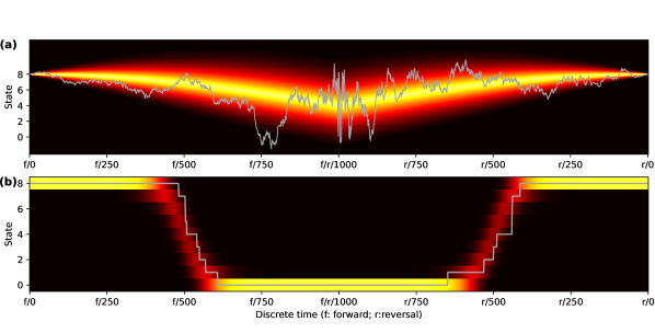
Figure 2: Probability distribution (heatmap) and paths (solid line) on a discrete-support $\Omega=\left\{0,1,\ldots M=8\right\}$. (a) Gaussian diffusion with de-quantization. The stochastic paths are not constrained on the discrete support, and also not bounded between $[0,M]$. Here, the Gaussian process is that in (Ho et al., 2020), with the cosine schedule. The forward process brings all the states to a high-dimensional Gaussian. (b) The discrete-state pure-death process takes place only on $\Omega$ and bring all the states to a $\delta$-distribution at $0$. Here, we used the discrete observation times specified in Appendix E. Both processes have $T=1000$ steps.

Note that Eq. (9) prescribes only the instantaneous time-dependent transition rates. Due to the simplicity of Blackout Diffusion, we can establish that the solution of the reverse-time process after a finite-time leap, i.e., $p_{(m,s)|(n,t),(o,0)}$, $0\leq s\leq t$, is also binomial in nature (see Appendix D):

$$p_{(m,s)|(n,t),(o,0)}={} \left(\begin{array}[]{c}o-n\\ m-n\end{array}\right)r^{m-n}(1-r)^{o-m},$$ (12)

$$r:={} s\left(e^{-s}-e^{-t}\right)/\left(1-e^{-t}\right).$$ (13)

In more compact notation, this can be written $X_{s}|(X_{0},X_{t})-X_{t}\sim\text{Binom}\left(X_{0}-X_{t},r\right)$. We label Eq. (13) as the Binomial bridge formula, since it is analogous to the key Brownian bridge formula used in Gaussian Generative Diffusion Models. Since we chose an independent decay process for each feature in the image data, all of the above can be immediately transferred from pixels $X\in\Omega$ to full images $\mathbf{X}\in\Omega^{N}$.

2.6 Diffusion Schedule and Loss functions

For training, a set of $T$ observation times $t_{k}\in\mathbb{R}_{\geq 0}$, $k=1,\ldots T$ is defined a priori, ordered by $0<t_{1}<t_{2}\ldots t_{T}$. In addition, $t_{0}:=0$. The choice of the observation times is analogous to the noise schedule in Gaussian diffusion models. Rather than treating the observation times/noise amplitudes as a hyperparameter to be optimized, as in Sohl-Dickstein et al. (2015); Nichol & Dhariwal (2021); Ho et al. (2020), we take a mathematical approach to defining the schedule of observation times $t_{k}$. The schedule is designed to uniformize the change in the Fisher information of the degraded samples, and this is derived in Appendix E.

Similar to other diffusion models, the goal is to train a neural network which transforms samples at $t_{k}$ to $t_{k-1}$. However, we accomplish this with a novel approach: Observing the instantaneous transition rate Eq. (9) and the finite reverse-time propagation Eq. (13), this goal can be achieved by training the neural net to predict the difference $\mathbf{X}_{0}-\mathbf{X}_{t_{k-1}}$, given a realization of $\mathbf{X}_{t_{k}}$. We will write the neural-net predicted difference as $\mathbf{y}:=\mathbf{NN}\left(\mathbf{X}_{t_{k}},t_{k}\right)$. We remark that this computational instantiation is drastically different from existing discrete diffusion implementations (Austin et al., 2021; Campbell et al., 2022) which model transition rates. With Blackout Diffusion, transition rates decays several orders of magnitudes, making it difficult to train a neural network to learn the transition rates. The remaining task is to establish the loss function that minimizes a metric on Eqs. (9) and (13).

We use a likelihood approach to define the loss function. Appendix F presents the derivation, showing that for a sample $\mathbf{X}_{t_{k}}$ generated by a particular training sample $\mathbf{X}_{0}$, the loss function can be defined as:

$$l_{i}=\left(t_{k}-t_{k-1}\right)e^{-t_{k}}\left[y_{i}-\left(\mathbf{X}_{0}-\mathbf{X}_{t_{k}}\right)_{i}\log y_{i}\right],$$ (14)

where $i$ indexes components of the multidimensional state. A finite-time correction by the binomial bridge formula is

$$l_{i}={} \left(e^{-t_{k-1}}-e^{-t_{k}}\right)\left[y_{i}-\left(\mathbf{X}_{0}-\mathbf{X}_{t_{k}}\right)_{i}\log y_{i}\right].$$ (15)

We average over each component $i$, samples in the training set $\mathbf{X}_{0}$, and randomly sampled observation time index $k$; the full loss is $\mathcal{\ell}=\left\langle l_{i}\right\rangle_{\{\mathbf{X_{0}},k,i\}}$. Note that if one chooses a uniformly distributed observation times and if the time difference $\Delta:=t_{k}-t_{k-1}\ll 1$, Eq. (15) converges asymptotically to Eq. (14).

2.7 Generating sample images

For image generation, we chose $t_{T}=15$, a time that is deemed long enough to approximate $t\rightarrow\infty$, in which limit all initial states converged to 0 (i.e., all the images degrade to all black). More accurately speaking, $p_{(0,15)|(255,0)}>0.9999$. To generate samples, we start with an all-black image, use the trained neural network to predict $\mathbf{X}_{t_{0}}-\mathbf{X}_{t_{T}}$, clipped at 0 and 255. Then, we can either use the general $\tau$-leaping algorithm (Gillespie, 2001) (which is analogous to the Euler–Maruyama integrator for Itô SDEs (Kloeden & Platen, 1999)) to generate a Poisson random number, or exploit the analytically exact binomial bridge Eq. (13), whose applicability is limited to Blackout Diffusion. The former sampling approach is similar to integrating Itô SDE in (Song et al., 2021d), and the latter approach is analogous to the Denoising Diffusion Probabilistic Model (Ho et al., 2020). The drawn numbers are added to the all-black image to obtain $\mathbf{X}_{t_{T-1}}$. The procedure repeats until $\mathbf{X}_{0}$ is obtained.

We summarize the proposed training and inference methods in Algorithms 1 and 2. The algorithms can be generalized to accommodate arbitrary continuous-time and discrete-state Markov process in Appendix G.

Algorithm 1 Training Blackout Diffusion

  repeat

     $\mathbf{X}_{0}\leftarrow\mathbf{x}$, drawn from the training set

     Draw an index $k$ from $\left\{1,\ldots T\right\}$ uniformly

     $\mathbf{X}_{t}\sim\text{Binomial}\left(\mathbf{X}_{0},e^{-t_{k}}\right)$ (element-wise)

     $\mathbf{y}\leftarrow\mathbf{NN}_{\theta}\left(\mathbf{X}_{t_{k}},k\right)$

     if Using instantaneous loss function Eq. (14) then

        $\omega_{k}\leftarrow\left(t_{k}-t_{k-1}\right)e^{-t_{k}}$

     else if Using finite-time loss function Eq. (15) then

        $\omega_{k}\leftarrow e^{-t_{k-1}}-e^{-t_{k}}$

     end if

     $l\leftarrow\omega_{k}\times\text{mean}\left\{\mathbf{y}-\left(\mathbf{X}_{0}-\mathbf{X}_{t_{k}}\right)\log\mathbf{y}\right\}$

     Take a gradient step on $\nabla_{\theta}l$

  until Converged

Algorithm 2 Generating images by Blackout Diffusion

  Initiate a blacked-out image $\mathbf{X}_{t_{T}}=0$

  for $k=T$ to $1$ do

     $\mathbf{y}_{\theta}\leftarrow\text{clip}\left(\mathbf{NN}_{\theta}\left(\mathbf{X}_{t_{k}},k\right),\,\mathbf{0},\,255\mathbf{I}-\mathbf{X}_{t_{k}}\right)$

     if Using Poisson then

        $\mathbf{d}\sim\text{Poisson}\left(\mathbf{y}_{\theta}\frac{e^{-t_{k}}}{1-e^{-t_{k}}}\right)$ (element-wise)

        $\mathbf{X}_{t_{k-1}}\leftarrow\text{clip}\left(\mathbf{X}_{t_{k}}+\mathbf{d},\mathbf{0},255\mathbf{I}\right)$

     else if Using Binomial Bridge then

        $\mathbf{d}\sim\text{Binomial}\left(\mathbf{y}_{\theta},\frac{e^{-t_{k-1}}-e^{-t_{k}}}{1-e^{-t_{k}}}\right)$ (element-wise)

        $\mathbf{X}_{t_{k-1}}\leftarrow\mathbf{X}_{t_{k}}+\mathbf{d}$

     end if

  end for

Table 1: Results of the numerical experiments (iteration 300K).

Loss	Sampling	FID	IS
Instantaneous	Binomial	4.77	9.01
Instantaneous	Poisson	4.92	9.18
Finite-time	Binomial	4.83	9.00
Finite-time	Poisson	5.01	9.08

Table 2: Summary of discrete methods

Dataset	Discrete Methods	Starts from a singular point?	Corrector steps	Time homogeneous	FID (↓)
	D3PM Absorbing (Austin et al., 2021)	$\checkmark$	None	$\times$	30.97
	D3PM Gauss (Austin et al., 2021)	$\times$	None	$\times$	7.34
CIFAR10	$\tau$LDR-0 (Campbell et al., 2022)	$\times$	None	$\times$	8.10
	$\tau$LDR-10 (Campbell et al., 2022)	$\times$	10	$\times$	3.74
	BlackOut (Ours)	$\checkmark$	None	$\checkmark$	4.77
	BlackOut (Ours)	$\checkmark$	2	$\checkmark$	4.58
Binarized MNIST	BlackOut (Ours)	$\checkmark$	None	$\checkmark$	0.02
CelebA	BlackOut (Ours)	$\checkmark$	None	$\checkmark$	3.21

3 Numerical Experiments

We chose the CIFAR-10 dataset to validate the feasibility of using Blackout Diffusion for generative modeling. We stress that our goal is to provide evidence that the theoretical results for discrete-state diffusion, derived above, are useful for practical tasks, rather than to advance the state-of-the-art for CIFAR-10 or any other dataset. To do so, we adopted the improved Noise Conditional Score Network (NCSN++) architecture presented in Song et al. (2021d, c) to serve the $\mathbf{NN}$ function in Eqs. (14) and (15). We made two minimal modifications on NCSN++ which bring the architecture in line with the theoretical requirements of Blackout Diffusion Modeling. (1) We applied a softplus function on the output of NCSN++ to ensure the positivity of the output. This is because the target ($\mathbf{X}_{0}-\mathbf{X}_{t_{k}}\geq 0$) is non-negative in Blackout Diffusion. (2) For inference, we clip the output of $\text{softplus}\left(\text{NCSN++}\left(\cdot\right)\right)$ by 0 and $255\mathbf{I}-\mathbf{X}_{t_{k}}$, followed by a round-off to the nearest integer. We used mini-batches with $256$ samples, and the training was stopped at 300K iterations, above which we observed degraded quality of the generated samples. We did not modify other hyperparameters of the NSCN++. We fixed $T=1000$ in this feasibility experiment. We performed the analysis on both loss functions, Eqs. (14) and Eq. (15), and by both binomial and Poisson sampling. The training was carried out by two NVIDIA A100 GPUs for $\sim$72 hr. Due to limited computational resources, we only trained once for each loss function. We then generated 50K samples, which took approximately 10.5 hours.

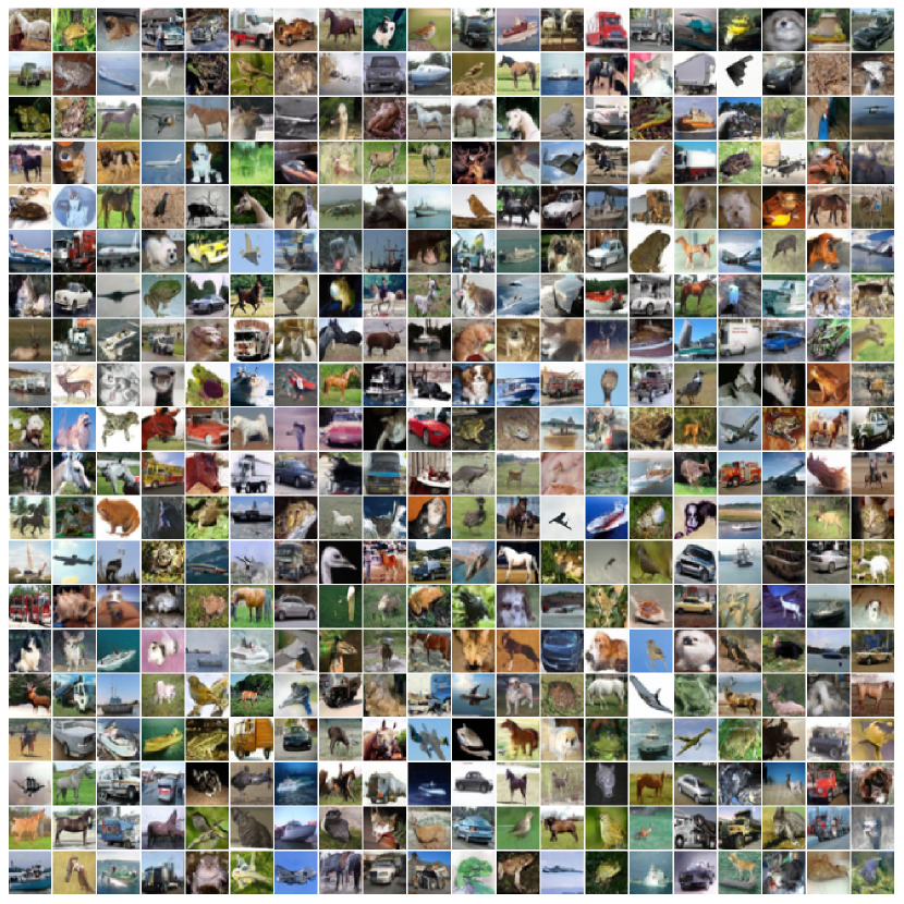
Figure 7: Four hundred samples generated by Blackout Diffusion trained by the finite-time loss function Eq. (15) and generated by the binomial bridge formula Eq. (13) during inference.

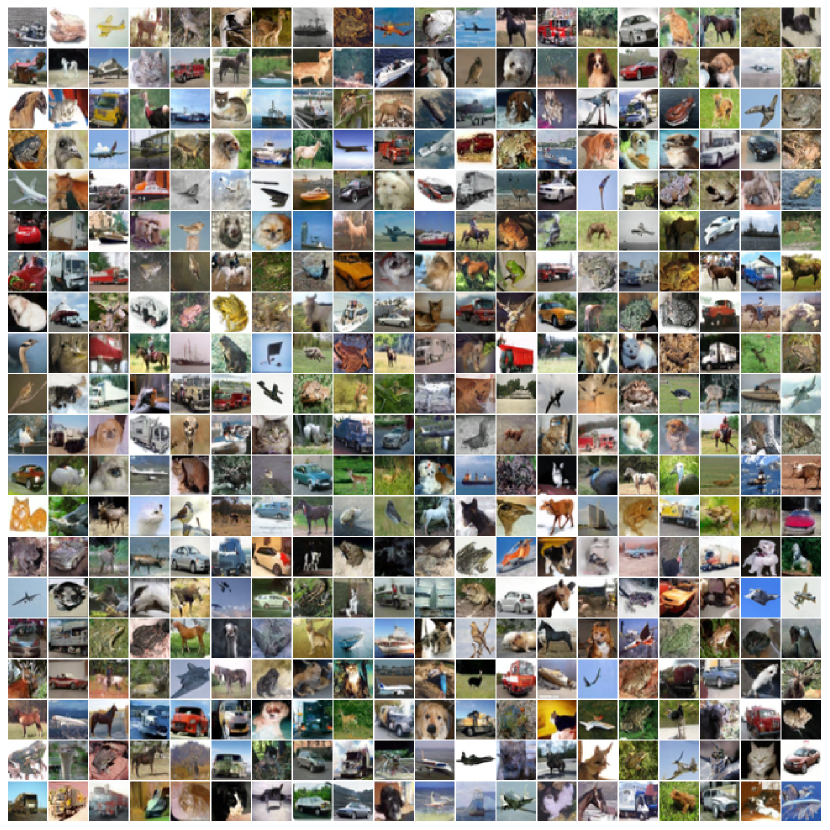
Figure 8: Four hundred samples generated by Blackout Diffusion trained by the finite-time loss function Eq. (15) and generated by $\tau$-leaping (Poisson random number) during inference.

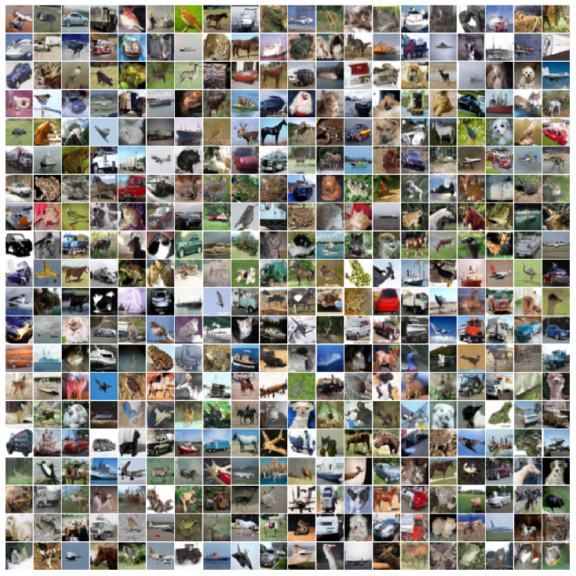
Figure 9: Four hundred samples generated by Blackout Diffusion trained by the instantaneous loss function Eq. (14) and generated by the binomial bridge formula Eq. (13) during inference.

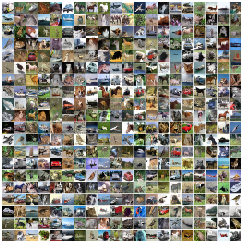
Figure 10: Four hundred samples generated by Blackout Diffusion trained by the instantaneous loss function Eq. (14) and generated by $\tau$-leaping (Poisson random number) during inference.

Selected samples are visualized in Fig. 3, which shows how the Blackout Diffusion Model generates different images from the same terminal condition ($\mathbf{X}_{t_{T}}=0$). Using 50K generated images, we computed the Fréchet Inception Distance (FID) to the training set and the Inception score (IS) in Table 1. Our results suggest that the quality of the generated samples is not sensitive to the choice of the loss function, and using the binomial bridge formula for sampling is slightly advantageous. We visualize 400 generated images for each case in Figs. 7-10. Results of binary MNIST and CelebA are shown in Table 2 and Figs. 11-13.

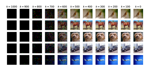
Figure 3: Image generation based on Blackout Diffusion. The color is adjusted per-image to better visualize the noisy signal at large times. Fig. 6 shows images with unadjusted colormap.

4 Discussion and Conclusion

We developed an exact theoretical framework for general discrete-state Markov processes, on either discrete- or continuous-time domain, which enables the exploration of Diffusion Modeling using a large class of stochastic processes. Our theoretical formulation for the discrete-state processes is analogous to Anderson (1982) for Gaussian processes. To the authors’ knowledge, a complete analogous theory for general discrete-state Markov processes has not yet been proposed. These theoretical results can be summarized as such: (1) We generalized the diffusion models based on those SDEs whose underlying noise is Wiener process (Song et al., 2021d) to discrete-state Markov processes. Besides yielding Blackout Diffusion based on the pure-death process, this paves the way to include more complex stochastic processes that involve some discreteness, e.g., jump-diffusion model (Huang et al., 2014), piecewise-deterministic Markov process (Faggionato et al., 2009), Gaussian diffusion with Markov switching (Mao & Yuan, 2006). Some of these more complex models could expand the current extent of generative diffusion models. (2) We derived the discrete-state score functions, Eqs. (6) and (45). These functions are analogous to the Stein score function (Song & Ermon, 2019). Since the score function was not used for training Blackout Diffusion, it remains for future work to see if score-based Diffusion Modeling (Song et al., 2021d; Song & Ermon, 2019) can be applied to discrete-state processes. For generic discrete-state models, the reverse-time generator Eq. (5) holds the key to enable FHDM (our Eq. (5) is the discrete-state counterpart of the continuous-state Itô SDE (9) in Ye et al. (2022)). FHDM uses distinct training and sampling methods based on Doob’s transformation to achieve improved quality and efficiency. Although in this paper we did not combine our theoretical formulation and FHDM, such a combination can be a fruitful research direction. Furthermore, as established in Ye et al. (2022), FHDM can be connected to the (continuous-state) Schrödinger–F:̈ollmer bridge formalism (Vargas et al., 2023, 2021; De Bortoli et al., 2021) and the (continuous-state) Path Integral Sampler (Zhang & Chen, 2022), we hypothesize that a successful application of our theoretical formulation to FHDM could initiate a new class of problems on corresponding discrete-state Schrödinger–Föllmer bridge and Path Integral formalism, which to our best knowledge do not exist yet. (3) We associate the “noise schedules” to the observation times of a continuous-time diffusion process. Such an association allowed us to design a principled, albeit heuristic, argument to construct the observation times based on Fisher information of the forward process. We remark that a different heuristic existed for training Mask Diffusion (Austin et al., 2021). (4) Using the exact theoretical formulation, we formulated a loss function based on maximum likelihood. This contrasts to Campbell et al. (2022), who took an approximate (variational) approach and then send the discrete time step down to zero. Our result (in Appendix G) shows that the variational bound in Campbell et al. (2022) is tight in the continuum-time limit. Finally, (4) we provide a demonstration that discrete-state Diffusion Modeling can be effective while exhibiting completely different qualitative behavior from Gaussian diffusion, by learning a Blackout Diffusion model on binarized MNIST, CIFAR-10, and CelebA-64.

These results also allow us to address conceptual questions about the technique of Diffusion Modeling more broadly:

Is Gaussian noise special? Our numerical experiment on Blackout Diffusion shows that Gaussian noise is not a crucial property for generative diffusion modeling. The discrete-state (Poissonian) noise in Blackout Diffusion can also be used for Generative Diffusion Modeling. This discovery is in line with a few other recently proposed models, e.g., Cold Diffusion Bansal et al. (2022) and Multinomial Diffusion Hoogeboom et al. (2021); Song et al. (2021a). Beyond the computational experiments, the existence of the generic instantaneous loss formula implies that the learning is tractable for any discrete-state process.
Must the forward and reverse processes correspond to noisifying and de-noising, respectively? Often, the forward process is described as one adds noise to the image (Ho et al., 2020; Hoogeboom et al., 2021). Blackout Diffusion highlights that this association must be taken with some subtlety. If noise corresponds to variance in the data across the space of samples of the stochastic process, for $t<\log 2$, the forward process for Blackout Diffusion adds noise, but for $t>\log 2$, the forward process removes noise as samples converge towards a blank image. The scenario is, of course, the reverse in the process of generating an image. As such, the first phase of inference involves adding noise to the sample. However, the whole forward (respectively, reverse) Blackout Diffusion is a degradation (reconstruction) process that removes (adds) information of the generated samples. This represents an apparent paradox: information is constantly diffusing away, despite the fact that all the pixels are converging to the same singular distribution, which has maximal information in the sense of Shannon entropy. As such, to declare whether a process is adding noise or removing noise critically depends on what type of stochastic process is used, and how noise is defined. Notably, the same phenomenon can be observed in Mask Diffusion, although the “denoisng” nature was not discussed (Austin et al., 2021). In light of this, we find it more accurate to simply declare that the forward and reverse processes are stochastic processes.
Does the final state $\mathbf{X}_{t_{T}}$ constitute a latent-space representation? The final state of the forward process is sometimes conceived as a latent-space representation, e.g., see Song et al. (2021d). Under this view, Diffusion Modeling appears conceptually very similar to Variational Autoencoders (Kingma & Welling, 2014) or Normalizing Flows (Rezende & Mohamed, 2015). However, both Mask Diffusion (Austin et al., 2021) and Blackout Diffusion converges all data to a single discrete point. Therefore, it seems impossible to conceive of the terminal space of the forward process as constituting a latent representation of the data. This highlights a fundamental difference between Diffusion Modeling and deterministic generative modeling. We argue that $\mathbf{X}_{t_{T}}$ is not a latent space, but the path-based conception of Rombach et al. (2022), where ($\mathbf{X}_{t_{1\ldots T-1}}$) may be viewed as a latent representation of the data—although this joint space is far larger than the original state space. With the similar spirit, we argue that the Cold Diffusion (Bansal et al., 2022) is more a flow model than a diffusion model because it cannot be directly applied to singular priors.

Finally, we would like to remark on the motivations that gave rise to our results and on future work that might be built from them. These results, collectively, arose out of the Authors’ endeavor to understand the theory behind Diffusion Modeling—like many Machine Learning advancements, a fairly complex foundational idea yields, in practice, a few simple formulas to implement. A great many recent works have treated the exploration of Diffusion Modeling as a problem of hyperparameters. Practical but ad hoc processes such as dequantization/requantization, and noise schedules have been included in pursuit of an engineering goal to improve model performance, but these stray significantly from the theoretical framework governing the underlying learning task. However, when looking at fundamentally different data domains—including but not limited to the discrete-space examples laid out in our introduction—this line of attack will likely introduce even machine learning algorithms for which the success cannot be explained and replicated. We believe that ad hoc procedures which improve performance are less likely to transfer across tasks or even individual datasets. In contrast, when a clear theoretical framework is provided, the individual pieces of the learning task, such as the forward evolution, reverse process, and loss function, can be more closely examined and tested, and the exploration of innovations can be driven by understanding in addition to empirical testing.

Having laid out the exact theoretical framework, discrete-space Diffusion Modeling thus presents many well-motivated opportunities. For example, we hypothesize that with further work, discrete-space Diffusion Models may be found that are far more computationally efficient than Gaussian Diffusion Models, because the state space is far smaller (mathematically, infinitely so) than in the continuous case. An empirical hint that this may be so comes from the fact that we adopted an existing continuous-space architecture (NCSN++) out-of-the-box and achieved reasonable results; further search of the space of network architectures and hyperparameters ought to yield some improvement.

Another advantage of our framework is that the instantaneous loss, Eq. (14), can be applied without any bridge formula that prescribes the reverse process analytically. Yet another advantage is in the computational tractability of the forward solution. For Gaussian Diffusion, the forward process is only computationally tractable because it can be analytically solved, and other continuous-state process which cannot be analytically solved are not computationally tractable. However, the forward evolution of discrete-state is very often numerically tractable, ask it involves powers (discrete-time) or exponentiation (continuous-time) of the transition matrix. These can be efficiently computed, e.g. by the Krylov subspace method (Saad, 1992; Gaudreault et al., 2018), bypassing the need for an analytical forward solution. Because of both of these advantages, we anticipate a rich library of discrete-state processes that can be used for diffusion modeling, and hope that these processes can be tailor-matched to the rich space of discrete-state data and systems that arise in the natural world.

Reproducibility and code availability

The codes we developed to perform the experiments are deposited at https://github.com/lanl/Blackout-Diffusion, with a C-number C23047 approved by the Richard P. Feynman Center for Innovation (FCI) at the Los Alamos National Laboratory.

Appendix A Deriving the Reverse-Time Evolutions

We first derive the reverse-time evolution for the continuous-time process (3). With $0\leq s\leq t$, recall that the conditional probabilities

$$p_{(m,s),(n,t)|(o,0)}=p_{(n,t)|(m,s),(o,0)}p_{(m,s)|(o,0)}=p_{(n,t)|(m,s)}p_{(m,s)|(o,0)}.$$ (16)

We use the Markov property $p_{(n,t)|(m,s),(o,0)}=p_{(n,t)|(m,s)}$ to establish the last equality. Applying $-\text{d}/\text{d}s$ to the equation above and by the chain rule, we arrive at

$$-\frac{\text{d}}{\text{d}s}p_{(m,s),(n,t)|(o,0)}={} -\frac{\text{d}p_{(n,t)|(m,s)}}{\text{d}s}p_{(m,s)|(o,0)}-p_{(n,t)|(m,s)}\frac{\text{d}p_{(m,s)|(o,0)}}{\text{d}s}$$

$$={} \nu_{\sigma}(m)p_{(m,s)|(o,0)}\left(\mathcal{E}_{\sigma}-1\right)p_{(n,t)|(m,s)}-p_{(n,t)|(m,s)}\left(\mathcal{E}_{\sigma}^{\dagger}-1\right)\left[\nu_{\sigma}(m)\,p_{(m,s)|(o,0)}\right]$$ (17)

by the forward and backward equations (3) and (4). Next, we apply the product identity to the terms involving the forward equation

$$-p_{(n,t)|(m,s)}\left(\mathcal{E}_{\sigma}^{\dagger}-1\right)\left[\nu_{\sigma}(m)\,p_{(m,s)|(o,0)}\right]={} -\left(\mathcal{E}_{\sigma}^{\dagger}-1\right)\left[p_{(n,t)|(m,s)}\nu_{\sigma}(m)\,p_{(m,s)|(o,0)}\right]$$

$$+\left\{\mathcal{E}_{\sigma}^{\dagger}\left[\nu_{\sigma}\left(m\right)p_{(m,s)|(o,0)}\right]\right\}\left\{\left(\mathcal{E}_{\sigma}^{\dagger}-1\right)p_{(n,t)|(m,s)}\right\},$$ (18)

to expand Eq. (17):

$$-\frac{\text{d}}{\text{d}s}p_{(m,s),(n,t)|(o,0)}={} \nu_{\sigma}(m)p_{(m,s)|(o,0)}p_{(n,t)|(\mathcal{E}_{\sigma}\left[m\right],s)}-\nu_{\sigma}(m)p_{(n,t)|(m,s)}p_{(m,s)|(o,0)}$$

$$-\left(\mathcal{E}_{\sigma}^{\dagger}-1\right)\left[p_{(n,t)|(m,s)}\nu_{\sigma}(m)\,p_{(m,s)|(o,0)}\right]$$

$$+\nu_{\sigma}\left(\mathcal{E}_{\sigma}^{\dagger}\left[m\right]\right)p_{(\mathcal{E}_{\sigma}^{\dagger}\left[m\right],s)|(o,0)}p_{(n,t)|(\mathcal{E}_{\sigma}^{\dagger}\left[m\right],s)}$$

$$-\nu_{\sigma}\left(\mathcal{E}_{\sigma}^{\dagger}\left[m\right]\right)p_{(\mathcal{E}_{\sigma}^{\dagger}\left[m\right],s)|(o,0)}p_{(n,t)|(m,s)}.$$ (19)

Next, note that three of the terms in the RHS of Eq. (19) cancel due to the identity

$$\left(\mathcal{E}_{\sigma}^{\dagger}-1\right){} \left[\nu_{\sigma}(m)p_{(n,t)|(m,s)}p_{(m,s)|(o,0)}\right]=$$

$$\nu_{\sigma}\left(\mathcal{E}_{\sigma}^{\dagger}\left[m\right]\right)p_{(\mathcal{E}_{\sigma}^{\dagger}\left[m\right],s)|(o,0)}p_{(n,t)|(\mathcal{E}_{\sigma}^{\dagger}\left[m\right],s)}-\nu_{\sigma}(m)p_{(n,t)|(m,s)}p_{(m,s)|(o,0)},$$ (20)

Eq. (19) can be simplified

$$-\frac{\text{d}}{\text{d}s}p_{(m,s),(n,t)|(o,0)}={} \nu_{\sigma}(m)p_{(m,s)|(o,0)}p_{(n,t)|(\mathcal{E}_{\sigma}\left[m\right],s)}-\nu_{\sigma}\left(\mathcal{E}_{\sigma}^{\dagger}\left[m\right]\right)p_{(\mathcal{E}_{\sigma}^{\dagger}\left[m\right],s)|(o,0)}p_{(n,t)|(m,s)}$$

$$={} \left(\mathcal{E}_{\sigma}-1\right)\left[\nu_{\sigma}\left(\mathcal{E}_{\sigma}^{\dagger}\left[m\right]\right)p_{(\mathcal{E}_{\sigma}^{\dagger}\left[m\right],s)|(o,0)}p_{(n,t)|(m,s)}\right],$$ (21)

by the identity of any step operators $\mathcal{E}_{\sigma}\mathcal{\mathcal{E}_{\sigma}^{\dagger}}=1$. Next, multiplying and dividing $p_{(m,s)|(o,0)}$ leads to the evolutionary equation of the joint ($(m,s)$ and $(n,t)$) conditional (on initial condition $(o,0)$)

$$-\frac{\text{d}}{\text{d}s}p_{(m,s),(n,t)|(o,0)}={} \left(\mathcal{E}_{\sigma}-1\right)\left[\nu_{\sigma}\left(\mathcal{E}_{\sigma}^{\dagger}\left[m\right]\right)\frac{p_{(\mathcal{E}_{\sigma}^{\dagger}\left[m\right],s)|(o,0)}}{p_{(m,s)|(o,0)}}p_{(n,t)|(m,s)}p_{(m,s)|(o,0)}\right]$$

$$={} \left(\mathcal{E}_{\sigma}-1\right)\left[\nu_{\sigma}\left(\mathcal{E}_{\sigma}^{\dagger}\left[m\right]\right)\frac{p_{(\mathcal{E}_{\sigma}^{\dagger}\left[m\right],s)|(o,0)}}{p_{(m,s)|(o,0)}}p_{(n,t),(m,s)|(o,0)}\right].$$ (22)

which is a closed-form evolution of the joint distribution $p_{(n,t),(m,s)|(o,0)}$, given the forward solution $p_{(m,s)|(o,0)}$. Finally, we divide both side of the equation on a particular terminal probability $p_{(n,t)|(o,0)}$ (assumed finite) to obtain Eq. (5):

$$-\frac{\text{d}}{\text{d}s}p_{(m,s)|(n,t),(o,0)}=\left(\mathcal{E}_{\sigma}-1\right)\left[\nu_{\sigma}\left(\mathcal{E}_{\sigma}^{\dagger}\left[m\right]\right)\frac{p_{(\mathcal{E}_{\sigma}^{\dagger}\left[m\right],s)|(o,0)}}{p_{(m,s)|(o,0)}}p_{(m,s)|(n,t),(o,0)}\right].$$ (23)

The derivation of the reverse-time evolution for the discrete-time process mostly follows the above derivation, but with a few additional technical details. With discrete-time index $k,\ell\in\mathbb{Z}_{\geq 0}$, $k<\ell$, the forward and backward equations read

$$p_{(m,k+1)|(o,0)}={} p_{(m,k)|(o,0)}+\left(\mathcal{E}_{\sigma}^{\dagger}-1\right)\left[\mu_{\sigma}(m)\,p_{(m,k)|(o,0)}\right],$$ (24)

$$p_{(n,T)|(m,k)}={} p_{(n,T)|(m,k+1)}+\mu_{\sigma}(m)\left(\mathcal{E}_{\sigma}-1\right)p_{(n,T)|(m,k+1)},$$ (25)

where $\mu_{\sigma}(m)$ is the transition probability from state $m$ to $m+\sigma\cdot 1$. We first express the conditional probabilities $p_{(m,k),(n,\ell)|(o,0)}=p_{(n,\ell)|(m,k)}p_{(m,k)|(o,0)}$; again, the Markov property $p_{(n,\ell)|(m,k),(o,0)}=p_{(n,\ell)|(m,k)}$ is used. Next, we establish an expression that is analogous to Eq. (17):

$$p_{(m,k),(n,\ell)|(o,0)}-p_{(m,k+1),(n,\ell)|(o,0)}=p_{(n,\ell)|(m,k)}p_{(m,k)|(o,0)}-p_{(n,\ell)|(m,k+1)}p_{(m,k+1)|(o,0)}$$

$$={} -p_{(m,k)|(o,0)}\left[p_{(n,\ell)|(m,k+1)}-p_{(n,\ell)|(m,k)}\right]+p_{(n,\ell)|(m,k+1)}\left[p_{(m,k)|(o,0)}-p_{(m,k+1)|(o,0)}\right]$$

$$={} p_{(m,k)|(o,0)}\mu_{\sigma}(m)\left(\mathcal{E}_{\sigma}-1\right)p_{(n,\ell)|(m,k+1)}-p_{(n,\ell)|(m,k+1)}\left(\mathcal{E}_{\sigma}^{\dagger}-1\right)\left[\mu_{\sigma}(m)\,p_{(m,k)|(o,0)}\right],$$ (26)

where the last equality was established by the forward and backward equations, (24) and (25). Next, we use the product identity to the terms involving the forward equation

$$-p_{(n,\ell)|(m,k+1)}\left(\mathcal{E}_{\sigma}^{\dagger}-1\right)\left[\mu_{\sigma}(m)\,p_{(m,k)|(o,0)}\right]$$

$$={} -\left(\mathcal{E}_{\sigma}^{\dagger}-1\right)\left[p_{(n,\ell)|(m,k+1)}\mu_{\sigma}(m)\,p_{(m,k)|(o,0)}\right]+\left[\mathcal{E}_{\sigma}^{\dagger}\left(\mu_{\sigma}(m)\,p_{(m,k)|(o,0)}\right)\right]\left[\left(\mathcal{E}_{\sigma}^{\dagger}-1\right)p_{(n,\ell)|(m,k+1)}\right]$$ (27)

to expand (26):

$$p_{(m,k),(n,\ell)|(o,0)}-p_{(m,k+1),(n,\ell)|(o,0)}={} p_{(m,k)|(o,0)}\mu_{\sigma}(m)\left(\mathcal{E}_{\sigma}-1\right)p_{(n,\ell)|(m,k+1)}$$

$$-\left(\mathcal{E}_{\sigma}^{\dagger}-1\right)\left[p_{(n,\ell)|(m,k+1)}\mu_{\sigma}(m)\,p_{(m,k)|(o,0)}\right]$$

$$+\left[\mathcal{E}_{\sigma}^{\dagger}\left(\mu_{\sigma}(m)\,p_{(m,k)|(o,0)}\right)\right]\left[\left(\mathcal{E}_{\sigma}^{\dagger}-1\right)p_{(n,\ell)|(m,k+1)}\right]$$

$$={} p_{(m,k)|(o,0)}\mu_{\sigma}(m)p_{(n,\ell)|(\mathcal{E}_{\sigma}\left[m\right],k+1)}-p_{(m,k)|(o,0)}\mu_{\sigma}(m)p_{(n,\ell)|(m,k+1)}$$

$$-\left(\mathcal{E}_{\sigma}^{\dagger}-1\right)\left[p_{(n,\ell)|(m,k+1)}\mu_{\sigma}(m)\,p_{(m,k)|(o,0)}\right]$$

$$+\mu_{\sigma}(\mathcal{E}_{\sigma}^{\dagger}\left[m\right])\,p_{(\mathcal{E}_{\sigma}^{\dagger}\left[m\right],k)|(o,0)}p_{(n,\ell)|(\mathcal{E}_{\sigma}^{\dagger}\left[m\right],k+1)}$$

$$-\mu_{\sigma}(\mathcal{E}_{\sigma}^{\dagger}\left[m\right])\,p_{(\mathcal{E}_{\sigma}^{\dagger}\left[m\right],k)|(o,0)}p_{(n,\ell)|(m,k+1)}.$$ (28)

The above expanded equation can be simplified by the identity

$$\left(\mathcal{E}_{\sigma}^{\dagger}-1\right)\left[p_{(n,\ell)|(m,k+1)}\mu_{\sigma}(m)\,p_{(m,k)|(o,0)}\right]={} p_{(n,\ell)|(\mathcal{E}_{\sigma}^{\dagger}\left[m\right],k+1)}\mu_{\sigma}(\mathcal{E}_{\sigma}^{\dagger}\left[m\right])\,p_{(\mathcal{E}_{\sigma}^{\dagger}\left[m\right],k)|(o,0)}$$

$$-p_{(n,\ell)|(m,k+1)}\mu_{\sigma}(m)\,p_{(m,k)|(o,0)},$$ (29)

leading to the reverse-time evolutionary equation for the joint conditional probabilities, analogous to Eq. (22):

$$p_{(m,k),(n,\ell)|(o,0)}-p_{(m,k+1),(n,\ell)|(o,0)}={} p_{(m,k)|(o,0)}\mu_{\sigma}(m)p_{(n,\ell)|(\mathcal{E}_{\sigma}\left[m\right],k+1)}-\mu_{\sigma}(\mathcal{E}_{\sigma}^{\dagger}\left[m\right])\,p_{(\mathcal{E}_{\sigma}^{\dagger}\left[m\right],k)|(o,0)}p_{(n,\ell)|(m,k+1)}$$

$$={} \left(\mathcal{E}_{\sigma}-1\right)\left[\mu_{\sigma}(\mathcal{E}_{\sigma}^{\dagger}\left[m\right])\,p_{(\mathcal{E}_{\sigma}^{\dagger}\left[m\right],k)|(o,0)}p_{(n,\ell)|(m,k+1)}\right]$$

$$={} \left(\mathcal{E}_{\sigma}-1\right)\left[\mu_{\sigma}(\mathcal{E}_{\sigma}^{\dagger}\left[m\right])\frac{p_{(\mathcal{E}_{\sigma}^{\dagger}\left[m\right],k)|(o,0)}}{p_{(m,k+1)|(o,0)}}p_{(n,\ell),(m,k+1)|(o,0)}\right].$$ (30)

Dividing both side by $p_{(n,\ell)|(o,0)}$ leads to:

$$p_{(m,k)|(o,0),(n,\ell)}=p_{(m,k+1)|(o,0),(n,\ell)}+\left(\mathcal{E}_{\sigma}-1\right)\left[\mu_{\sigma}(\mathcal{E}_{\sigma}^{\dagger}\left[m\right])\frac{p_{(\mathcal{E}_{\sigma}^{\dagger}\left[m\right],k)|(o,0)}}{p_{(m,k+1)|(o,0)}}p_{(m,k+1)|(o,0),(n,\ell)}\right],$$ (31)

which is the reverse-time stochastic process for the discrete-time and discrete-state Markov processes.

Remark 1. Both Eqs. (23) and (31) can be understood as the forward equation for the reverse-time process. Note that an overall operator $\mathcal{E}_{\sigma}-1$ is applied to the product of the transition rate and conditional probabilities (cf. the adjoint operator $\mathcal{E}_{\sigma}^{\dagger}-1$ in the forward equation of the forward process, Eqs. (24) and (3)). This indicates that the shift operators for the reverse-time process is adjoint to those in the forward process, meaning the possible transitions are opposite—a state $m$ later in time can only transit to a state $m^{\prime}_{\sigma}$ earlier in time, if a transition from $m^{\prime}_{\sigma}$ to $m$ is permitted in the forward process. Note, however, the transition rate (or probability) of the reverse-time $m\rightarrow m^{\prime}_{\sigma}$ is not identical to the transition rate (or probability) of the forward process $m_{\sigma}^{\prime}\rightarrow m$.

Remark 2. For the discrete-time system, it is possible to adopt an alternative derivation that is similar to (Sohl-Dickstein et al., 2015), without introducing the formal operator-algebraic derivation in this section. We are interested in deriving the probability $p_{(m^{\prime}_{\sigma},k)|(m,k+1),(o,0)}$. Using conditional Bayes formula, we can express

$$p_{(m^{\prime}_{\sigma},k)|(m,k+1),(o,0)}=\frac{p_{(m,k+1)|(m^{\prime}_{\sigma},k),(o,0)}p_{(m^{\prime}_{\sigma},k)|(o,0)}}{p_{(m,k+1)|(o,0)}}.$$ (32)

By the Markov property of the process, $p_{(m,k+1)|(m^{\prime}_{\sigma},k),(o,0)}p_{(m^{\prime}_{\sigma},k)|(o,0)}=p_{(m,k+1)|(m^{\prime}_{\sigma},k)}$, which is the transition probability $L_{mm^{\prime}_{\sigma}}$ (and $\nu_{\sigma}(m^{\prime}_{\sigma})$ in the context of process Eq. (24)). Thus, (32) prescribes the transition probabilities of the reverse-time evolution, which is described by Eq. (31).

Remark 3. A typical technique to derive continuous-time master equations is to consider a discrete-time Markov chain and express the transition probabilities in terms of continuous-time rate constants, $\mu_{\sigma}(m)=\nu_{\sigma}(m)\Delta t$, and sending $\Delta t\downarrow 0$. It is clear to see such treatment transforms Eq. (31) to Eq. (23).

Appendix B Generalization of the Theoretical Formulation for Arbitrary Discrete-State Markov Processes

In this section, we present the generalization for the continuous-time process, defined as the forward Chapman–Kolmogorov Equation (2). A parallel derivation for the discrete-time case (Eq. (24)) is omitted.

The key idea is to realize that the step operators $\mathcal{E}_{\sigma}$ are simply a way for us to reformulate the transition matrix $L$ in (2). Let us define rate functions for a general $n$-step transition (those transitions from $m$ to $m^{\prime}$ such that $|m-m^{\prime}|=n$):

$$\nu_{n,\sigma}(m):=\left\{\begin{array}[]{ll}L^{\dagger}_{m+\sigma n,m},&\text{if }m+\sigma\cdot n\in\Omega\\ 0,&\text{else.}\end{array}\right.$$ (33)

It suffices to consider $n=1,\ldots M$ for our setup (where the state in the finite-state space $\Omega$ is labeled from 1 to $M$). Then, Eq. (2) can be reformulated as a linear sum of powers of the shift operators

$$\frac{\text{d}}{\text{d}t}p_{(m,t)|(o,0)}=\left[\left(\mathcal{E}_{\sigma}^{\dagger}\right)^{n}-1\right]\left[\nu_{n,\sigma}\left(m\right)p_{(m,t)|(o,0)}\right].$$ (34)

We remind the reader that we used the Einstein summation convention to sum over $\sigma\in\left\{+,-\right\}$ and $n\in\left\{0,\ldots M\right\}$ in the above equation. Similarly, the Kolmogorov backward equation is

$$-\frac{\text{d}}{\text{d}s}p_{(n,t)|(m,s)}=\nu_{n,\sigma}\left(m\right)\left(\mathcal{E}_{\sigma}^{n}-1\right)p_{(n,t)|(m,s)}$$ (35)

As the powers of the step operators are still step operators, the procedure in Appendix A can be applied to deliver the reverse-time evolutionary equation:

$$-\frac{\text{d}}{\text{d}s}p_{(m,s)|(n,t),(o,0)}=\left[\nu_{n,\sigma}\left(m^{\prime}\right)\frac{p_{(m^{\prime},s)|(o,0)}}{p_{(m,s)|(o,0)}}p_{(m,s)|(n,t),(o,0)}\right],$$ (36)

where $m^{\prime}$ is again the pre-image $\left(\mathcal{E}_{\sigma}^{\dagger}\right)^{n}\left[m\right]$ of transition $(n,\sigma)$ mapping $m^{\prime}$ to $m$ forward in time.

Appendix C Kramers–Moyal expansion of the reverse-time evolution in discrete-state spaces

In this section, we aim to apply the Kramers–Moyal expansion (van Kampen, 2007; Gardiner, 2009; Weber & Frey, 2017) to the both the forward and reverse-time discrete-state process, Eq. (5) and (5) respectively. Albeit rather standard and straightforward, the analysis on the reversal process requires extra care compared to the usual practices, due to the fact that the (reverse-time) transition rate depends on non-local information (i.e., $\nu_{\sigma}$ is evaluated at the preimage of viable transitions to the state $m$).

As usual, we set out the analysis by asserting a large system size $V:=\mathcal{O}\left(X_{t}\right)\gg 1$. We denote the scaled variables by a tilde, for example, $\tilde{m}:=m/V$, $\tilde{n}:=n/V$, and $\tilde{o}:=o/V$. Similarly, the scaled rate constants $\tilde{\nu}_{\sigma}(\tilde{m}):=\nu_{\sigma}(m)/V$. The probabilities $p$’s now relate to a probability density $\rho$ in the continuum (state) limit, $p=\rho\text{d}x=\rho/V$, with $\text{d}x:=1/V\ll 1$. Now for any test function $f$ on the discrete-state space,

$$\left(\mathcal{E}_{\sigma}-1\right)f(m)=f\left(m+\sigma\cdot 1\right)-f(m)=V\tilde{f}\left(\tilde{m}+\sigma\cdot\frac{1}{V}\right).$$ (37)

With minor assumptions on the scaled test function $\tilde{f}$, it can be Taylor-expanded, which is the foundation of the Kramers–Moyal expansion, i.e.,

$$\left(\mathcal{E}_{\sigma}-1\right)f(m)=f\left(m+\sigma\cdot 1\right)-f(m)=V\tilde{f}\left(\tilde{m}\right)+\sigma\frac{\text{d}\tilde{f}}{\text{d}\tilde{m}}+\frac{1}{2V}\frac{\text{d}^{2}\tilde{f}}{\text{d}\tilde{m}^{2}}.$$ (38)

Per the constraints pointed out Pawula (1967), one usually asymptotically expands up to $\mathcal{O}\left(1/V^{2}\right)$ and truncates the higher orders to obtain the Fokker–Planck equation.

For the forward process, the expansion leads to the following Itô stochastic differential equation

$$\text{d}\tilde{X}_{t}=v\left(\tilde{X}_{t}\right)\text{d}t+\sqrt{D\left(\tilde{X}_{t}\right)}\text{d}W_{t},$$ (39)

where $\tilde{X}_{t}\approx X_{t}/V$ is the scaled continuum-state variable, $v(x):=\left[\nu_{+}(Vx)-\nu_{-}(Vx)\right]/V$ is the drift, and $D\left(x\right):=\left[{\nu}_{+}(Vx)+\nu_{-}(Vx)\right]/(2V^{2})$ is the diffusion. The forward solution of the discrete-state system, $p_{(m,t)|(o,0)}$, asymptotically converges to the solution of Eq. (39) in the continuum limit $M\gg 1$.

Performing the expansion for the reversal process Eq. (5) requires extra care. The complication from the fact that the transition rates inside the square brackets are non-local and requires asymptotic expansion, and a careful matching of the asymptotic orders is needed. We first rewrite the reverse-time transition rate

$$\nu_{\sigma}\left(\mathcal{E}_{\sigma}^{\dagger}\left[m\right]\right)\frac{p_{(\mathcal{E}_{\sigma}^{\dagger}\left[m\right],s)|(o,0)}}{p_{(m,s)|(o,0)}}=\left[\nu_{\sigma}\left(\mathcal{E}_{\sigma}^{\dagger}\left[m\right]\right)-\nu_{\sigma}\left(m\right)+\nu_{\sigma}\left(m\right)\right]\left[\frac{p_{(\mathcal{E}_{\sigma}^{\dagger}\left[m\right],s)|(o,0)}-p_{(m,s)|(o,0)}}{p_{(m,s)|(o,0)}}+1\right].$$ (40)

Asymptotically expanding difference terms in both brackets to $\mathcal{O}\left(1/V\right)$:

$$\nu_{\sigma}\left(\mathcal{E}_{\sigma}^{\dagger}\left[m\right]\right)-\nu_{\sigma}\left(m\right)={} \left(\mathcal{E}_{\sigma}^{\dagger}-1\right)\nu_{\sigma}\left(m\right)=-\sigma\frac{\text{d}\tilde{\nu}_{\sigma}}{\text{d}\tilde{m}}+\mathcal{O}\left(\frac{1}{V}\right),$$ (41a)

$$\frac{p_{(\mathcal{E}_{\sigma}^{\dagger}\left[m\right],s)|(o,0)}-p_{(m,s)|(o,0)}}{p_{(m,s)|(o,0)}}={} \frac{\left(\mathcal{E}_{\sigma}^{\dagger}-1\right)p_{(m,s)|(o,0)}}{p_{(m,s)|(o,0)}}$$

$$={} -\frac{\sigma}{V}\frac{1}{\rho\left(\tilde{m},s|\tilde{o},0\right)}\frac{\text{d}\rho\left(\tilde{m},s|\tilde{o},0\right)}{\text{d}\tilde{m}}+\mathcal{O}\left(\frac{1}{V}\right).$$ (41b)

A key detail of the analysis is that

$$\mathcal{O}\left(\frac{1}{\rho\left(\tilde{m},s|\tilde{o},0\right)}\frac{\partial\rho\left(\tilde{m},s|\tilde{o},0\right)}{\partial\tilde{m}}\right)=\mathcal{O}\left(\frac{\partial\log\left(\tilde{m}\right)}{\partial\tilde{m}}\right)=\mathcal{O}\left(V\right),$$ (42)

because the variance of the forward Gaussian diffusion $\rho\left(\tilde{m},s|\tilde{o},0\right)$ is of order $\mathcal{O}\left(1/V\right)$. We can now collect the leading ($\mathcal{O}\left(V^{1}\right)$) asymptotic expression of the transition rates in Eq. (40):

$$\nu_{\sigma}\left(\mathcal{E}_{\sigma}^{\dagger}\left[m\right]\right)\frac{p_{(\mathcal{E}_{\sigma}^{\dagger}\left[m\right],s)|(o,0)}}{p_{(m,s)|(o,0)}}=\nu_{\sigma}\left(m\right)\left[1-\frac{\sigma}{V}\frac{1}{\rho\left(\tilde{m},s|\tilde{o},0\right)}\frac{\text{d}\rho\left(\tilde{m},s|\tilde{o},0\right)}{\text{d}\tilde{m}}\right]+\mathcal{O}\left(V^{1}\right).$$ (43a)

As such, asymptotically speaking, the transition rates of the reverse-time process are almost identical to the forward process, except for the correction $\left(\sigma/V\right)\partial_{\tilde{m}}\rho\left(\tilde{m},s\right)$. The Kramers–Moyal expansion of the process (5) results in the standard Itô stochastic differential equation (39), with the drift $v$ and diffusion $D$ defined as

$$v\left(\tilde{m}\right)={} \sum_{\sigma\in\left\{+,-\right\}}\sigma\cdot\tilde{\nu}_{\sigma}\left(V\cdot\tilde{m}\right)\left[1-\frac{\sigma}{V}\frac{1}{\rho\left(\tilde{m},s|\tilde{o},0\right)}\frac{\text{d}\rho\left(\tilde{m},s|\tilde{o},0\right)}{\text{d}\tilde{m}}\right]$$

$$={} \left(\sum_{\sigma\in\left\{+,-\right\}}\sigma\cdot\tilde{\nu}_{\sigma}\left(V\cdot\tilde{m}\right)\right)-\frac{1}{V}\frac{1}{\rho\left(\tilde{m},s|\tilde{o},0\right)}\frac{\text{d}\rho\left(\tilde{m},s|\tilde{o},0\right)}{\text{d}\tilde{m}},$$ (44a)

$$D\left(\tilde{m}\right)={} \frac{1}{2V}\sum_{\sigma\in\left\{+,-\right\}}\tilde{\nu}_{\sigma}\left(V\cdot\tilde{m}\right).$$ (44b)

Note that the functional form of the correction in the drift $v$ is similar to that in Anderson (1982). Such a correction term is the key target for learning in the score-based generative models (Song & Ermon, 2019, 2020; Song et al., 2021d, b).

Remark 1. The analogous Stein score function (Song & Ermon, 2019, 2020; Song et al., 2021d, b) for the discrete-state system can be identified in the above analysis (see Eq. (40))

$$s_{\text{dis},\sigma}\left(m,s\right)\propto\nu_{\sigma}\left(\mathcal{E}^{\dagger}_{\sigma}\left[m\right]\right)\frac{p_{(\mathcal{E}_{\sigma}^{\dagger}\left[m\right],s)|(o,0)}-p_{(m,s)|(o,0)}}{p_{(m,s)|(o,0)}}$$ (45)

The asymptotic analysis shows in the dense-grid limit, the above finite-difference formula is asymptotically proportional to the Stein score function for continuous-sate system, $s_{\text{cts}}\left(m,s\right):=\partial_{\tilde{m}}\log\rho\left(\tilde{m},s\right)$. The proportionality came from the constant $1/V$, which is proportional to the variance of the forward solution. Such a proportionality constant is usually normalized in the score-based approaches, see discussion in Song et al. (2021d). It is straightforward to show that the score function of Blackout Diffusion Eq. (7) has an interesting functional form

$$\frac{1}{m+1}\left(\frac{oe^{-t}-m}{1-e^{-t}}-1\right).$$ (46)

We did not directly learn this function in this paper.

Remark 2. The discrete-state score functions Eq. (45) depends on the forward solution evaluated at the preimage $m^{\prime}=\mathcal{E}_{\sigma}^{\dagger}\left[m\right]$ of a viable transition to the state $m$. For general Markov transition process (see Appendix B) with $J$ viable transitions into state $m$ (i.e., $J$ non-zero $L^{\dagger}_{mm^{\prime}}$, $m\neq m^{\prime}$), there exists $J$ distinct score functions with the same functional form (45).

Appendix D Deriving the binomial bridge formula

The Binomial Bridge Formula (13) can be established straightforwardly. For $0\leq s\leq t$, Eq. (8) states

$$p_{(m,s)|(o,0)}={} \left(\begin{array}[]{c}o\\ m\end{array}\right)e^{-ms}\left(1-e^{-s}\right)^{o-m}$$ (49)

$$p_{(n,t)|(o,0)}={} \left(\begin{array}[]{c}o\\ n\end{array}\right)e^{-nt}\left(1-e^{-t}\right)^{o-n}.$$ (52)

In addition, the forward propagation from time $s$ to $t$ can be expressed in a similar form, by the Markov property of the process:

$$p_{(n,t)|(m,s)}=\left(\begin{array}[]{c}m\\ n\end{array}\right)e^{-n\left(t-s\right)}\left(1-e^{-\left(t-s\right)}\right)^{m-n}.$$ (53)

Applying conditional Bayes formula,

$$p_{(m,s)|(n,t),(o,0)}={} \frac{p_{(n,t)|(m,s),(o,0)}p_{(m,s)|(o,0)}}{p_{(n,t)|(o,0)}}=\frac{p_{(n,t)|(m,s)}p_{(m,s)|(o,0)}}{p_{(n,t)|(o,0)}}$$

$$={} \frac{\left(o-n\right)!}{\left(m-n\right)!\left(o-m\right)!}\frac{e^{-ms}\left(1-e^{-s}\right)^{o-m}e^{-n\left(t-s\right)}\left(1-e^{-\left(t-s\right)}\right)^{m-n}}{e^{-nt}\left(1-e^{-t}\right)^{o-n}}$$

$$={} \frac{\left(o-n\right)!}{\left(m-n\right)!\left(o-m\right)!}\left(\frac{1-e^{-s}}{1-e^{-t}}\right)^{o-m}\left(\frac{e^{-s}-e^{-t}}{1-e^{-t}}\right)^{m-n},$$ (54)

where we used the Markov property to establish the first equality. By defining $r:=\left(e^{-s}-e^{-t}\right)/\left(1-e^{-t}\right)$, the above equation can be succinctly expressed as

$$p_{(m,s)|(n,t),(o,0)}=\frac{\left(o-n\right)!}{\left(m-n\right)!\left(o-m\right)!}\left(1-r\right)^{o-m}r^{m-n},$$ (55)

which is the probability mass function of a binomial distribution.

Remark (the “physicists’ solution”). The Binomial Bridge Formula can be understood intuitively by the following argument. Consider $o$ radioactive particles going through a $\beta$ decay process. We are asked to infer how many are radioactive at time $s$, given that there are $n$ still active at time $t$. Another way to frame the condition is that at time $t$, there are $o-n$ already decayed. For any one of these particles, the conditional probability that it already decayed at time $s$ conditioned on that it decayed at time $t$ is $(1-e^{-s})/(1-e^{-t})$; equivalently, the conditional probability that it remained radioactive at time $s$ conditioned on that it decayed at time $t$ is $1-(1-e^{-s})/(1-e^{-t})=(e^{-s}-e^{-t})/(1-e^{-t})$. Because each particle goes through an independent process, among those $o-n$ which decayed at time $t$, $\text{Binom}\left(o-n,\left(e^{-s}-e^{-t}\right)/\left(1-e^{-t}\right)\right)$ remained radioactive at time $s$. Adding $n$ which has not decayed by time $t$, the total remaining population at time $s$ is thus $n+\text{Binom}\left(o-n,\left(1-e^{-s}\right)/\left(1-e^{-t}\right)\right)$ remaining.

Appendix E Observation times

The observation times $\left\{t_{k}\right\}_{k=1}^{T}$ specify when the realizations of the forward stochastic processes are generated. The choice of $\left\{t_{k}\right\}_{k=1}^{T}$, analogous to the noise schedules in Gaussian diffusion models (Sohl-Dickstein et al., 2015; Song et al., 2021d), is crucial to the quality of the trained generative model. Here, we present a heuristic way to design the observation times.

Our proposition is to adopt the Fisher information (FI) of the forward process as a guidance. The main idea is that we will use more observation times when the forward process (3) has higher FI. Recall that for the pure-death process (7), suppose the color pixel at $t=0$ is at a state $o\in\Omega$, at time $t$ the solution to the forward process is $\text{Binom}\left(o,q(t)\right)$, where the parameter $q(t)=\exp\left(-t\right)$. As such, the FI of parameter $q$ can be expressed

$$\text{FI}(q)=\frac{o}{q\left(1-q\right)}.$$ (56)

Importantly, the time-dependent part of the $\text{FI}(q)$ is identical for all initial configuration; the implicit dependence comes from $q(t)=\exp\left(-t\right)$. Next, let us define a probability distribution $\phi$ of the observation times in infinitely-many observation limit ($T\rightarrow\infty$), such that the corresponding density $\text{d}\phi$ is proportional to the time-dependent part of the FI:

$$\text{d}\phi\left(q\right)\propto\frac{1}{q\left(1-q\right)}.$$ (57)

With a change of variable from $q$ to $t$ by $q=e^{-t}$, the density function $\phi$ on the time domain is

$$\text{d}\phi\left(t\right)\propto\frac{e^{-t}}{e^{-t}\left(1-e^{-t}\right)}.$$ (58)

Note that the function $\text{d}\phi$ is symmetric about $t=\log(2)$, at which time the system is maximally noisy. Next, we use the inverse transform sampling to generate discrete observation times. The first step is to express the cumulative distribution function, obtained by integrating (58)

$$\text{CDF}(t)\propto\text{Logit}\left(e^{-t}\right)+const.$$ (59)

Note the apparent singularity as $t\downarrow 0$ and $t\uparrow\infty$. We bypass the singularity by a symmetry argument, that we would like to put exactly half of the discretization times before and after $\log(2)$, and the fact that the final time $t_{T}=15<\infty$ will be chosen. With the symmetry argument, the first finite time $t_{1}$ is determined to be $-\log\left(1-e^{t_{T}}\right)$. Then, we uniformly choose in between $\text{CDF}(t_{1})$ and $\text{CDF}(T)$ for the rest $t_{k}$’s, i.e.,

$$t_{k}=-\log\left[\sigma\left(\text{Logit}\left(1-e^{-t_{T}}\right)+\frac{k-1}{T-1}\left[\text{Logit}\left(e^{-t_{T}}\right)-\text{Logit}\left(1-e^{-t_{T}}\right)\right]\right)\right],\quad k=1,2,\ldots T,$$ (60)

where $\sigma(x)\equiv\text{Logit}^{-1}(x):=1/\left(1+e^{-x}\right)$ is the sigmoid function. Figure 4 shows the dependence of $t_{k}$ on $k$.

It is worth mentioning that we also experimented other heuristics, including replacing the Fisher Information by the entropy of the process, entropic production rate, variance, Kullback–Leibler divergence between observation times, signal-to-noise ratio metrics such as the coefficients of variation, and uniform temporal grid. Among all the heuristic methods we experimented, the Fisher Information performed significantly better.

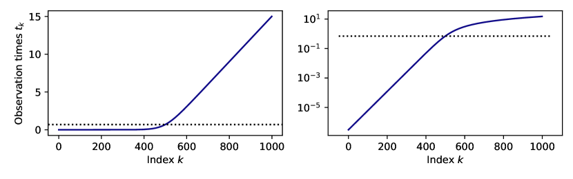
Figure 4: The observation times defined by Eq. (60), in (left panel) linear and (right panel) logarithmic scales. The dashed lines label the time $t=\log 2$, when the images are maximally noisified.

Appendix F Likelihood functions

In this section, we derive the loss function from the formal likelihood function of continuous-time and discrete-state system. It suffices to consider one transition (say, $m\rightarrow m^{\prime}$) with aground-truth transition rate $\lambda(t)$. In the limit of $\delta t\ll 1$, the probability of the state transition to $m^{\prime}$ is then $\lambda(t)\Delta t$ (van Kampen, 2007; Gardiner, 2009), and the probability of no transition event occurred is $1-\lambda(t)\Delta t$. More-than-one transition events can be ignored because they occur at higher order of $\mathcal{O}\left(\Delta t^{2}\right)$. Let us denote the model-predicted transition rate by $\kappa_{\theta}(t)$ which depends on model parameters $\theta$. The corresponding model predicted probabilities are $\kappa_{\theta}(t)\Delta t$ and $1-\kappa_{\theta}(t)\Delta t$. Now, the support of the viable state is only $\left\{m,m^{\prime}\right\}$, so the instantaneous (at time $t$) negative log-likelihood (NNL) can be easily formulated

$$-\text{NLL}(t)=\lambda(t)\Delta t\log\frac{\lambda(t)\Delta t}{\kappa_{\theta}(t)\Delta t}+\left(1-\lambda(t)\Delta t\right)\log\frac{1-\lambda(t)\Delta t}{1-\kappa_{\theta}(t)\Delta t}$$ (61)

which is the Kullback–Leibler divergence between the two Bernoulli distributions induced by the ground-truth and model-predicted processes at time $t$. Neglecting $\theta$-independent terms, and asymptotically expanding the second term on the RHS

$$-\left(1-\lambda(t)\Delta t\right)\log\left(1-\kappa_{\theta}(t)\Delta t)\right)=\kappa_{\theta}(t)\Delta t+\mathcal{O}\left(\Delta t^{2}\right),$$ (62)

we arrive at

$$-\text{NLL}(t)=\Delta t\left(\kappa_{\theta}(t)-\lambda(t)\log\kappa_{\theta}(t)\right)+(const.\text{ of }\theta).$$ (63)

Note that in the reversal process, both the ground-truth reversal rate (prescribed by Eq. (5)) and the model-predicted rate $\kappa_{\theta}$ are time-dependent, and we want to learn the whole process, formally $0\leq t<\infty$. Let us first consider the full negative log-likelihood in the continuum-time limit (i.e., infinitely many observation times) by integrating the above expression:

$$\text{Full NLL}=\int\left(\kappa_{\theta}\left(\tau\right)-\lambda\left(\tau\right)\log\kappa_{\theta}\left(\tau\right)\right)\text{d}\tau+(const.\text{ of }\theta).$$ (64)

In practice, the times are sampled in a Monte Carlo fashion, such that only one observation time is drawn for each drawn training image. Recall that we devised a sampling distribution, Eq.(58), based on a heuristic argument about Fisher information of the process in Appendix E. Similar to an importance sampler, each sample is reweighted by the probability density $\phi(t)$:

$$\text{Full NLL}=\int\phi\left(\tau\right)\left[\frac{1}{\phi\left(\tau\right)}\left(\kappa_{\theta}\left(\tau\right)-\lambda\left(\tau\right)\log\kappa_{\theta}\left(\tau\right)\right)\right]\text{d}\tau+(const.\text{ of }\theta).$$ (65)

This brought us to the loss function as

$$l=\frac{\Delta t}{\phi\left(\tau\right)}\left(\kappa_{\theta}-\lambda\log\kappa_{\theta}\right),$$ (66)

and by minimizing $l$ we can achieve maximization of the likelihood. For the Blackout Diffusion process, the reverse-time transition rate

$$\lambda=\left(X_{0}-X_{t_{k+1}}\right)\frac{\left(t_{k}-t_{k-1}\right)e^{-{t_{k}}}}{1-e^{-{t_{k}}}},$$ (67)

and as the neural net predicts also the difference $y=o-m$,

$$\kappa_{\theta}=y\times\frac{e^{-t_{k}}}{1-e^{-t_{k}}},$$ (68)

which leads to the expression (14), after neglecting another $\theta$-independent constant.

We next derive finite-time corrected loss function, Eq. (15). Note that the model predicted $\kappa_{\theta}$ can only be evaluated at a priori defined observation times, $t_{k}$’s. Using the (constant) rates predicted at time $t_{k}$ to evolve the system back to $t_{k-1}$ is identical to the $\tau$-leaping algorithm (Gillespie (2001); it is analogous to the Euler–Maruyama integration scheme for continuous-state systems). Without taking time-dependent rate constants into account, the constant-rate approach results in $X_{t_{k}}|\left(X_{0},X_{t_{k+1}}\right)-X_{t_{k}}\sim\text{Poisson}\left(\kappa_{\theta}\right)$, and forms only an approximation to the true binomial distribution D. In this case, we can still formulate the exact likelihood: assuming that at time $t_{k+1}$

$$-\log L=\sum_{j=m}^{M}\text{PMF}_{\text{GT}}\left(m\right)\log\frac{\text{PMF}_{\text{GT}}\left(m\right)}{\text{PMF}_{\theta}\left(m\right)},$$ (69)

where $\text{PMF}_{\text{GT}}$ is the ground-truth probability mass function of the binomial Eq. (13), and $\text{PMF}_{\theta}$ is the model-predicted probability mass function, i.e., $\text{Poisson}\left(\kappa_{\theta}\right)$. Inserting the expressions, we obtain

$$-\log L={} -\sum_{j=m}^{M}\text{PMF}_{\text{GT}}\left(m\right)\left[m\log\kappa_{\theta}-\kappa_{\theta}\right]+(const.\text{ of }\theta)$$

$$={} \kappa_{\theta}-\left[\sum_{j=m}^{M}m\text{PMF}_{\text{GT}}\left(m\right)\right]\log\kappa_{\theta}+(const.\text{ of }\theta)$$

$$={} \kappa_{\theta}-\left(o-m\right)\frac{e^{-t_{k-1}}-e^{-t_{k}}}{1-e^{-t_{k}}}\log\kappa_{\theta}+(const.\text{ of }\theta).$$ (70)

Since the neural net was used to predict $o-m$, we obtain (15), after discounting the distribution $1/\phi$.

Appendix G Algorithms for general continuous-time discrete-state Markov processes

With a little more effort, it is possible to prescribe algorithms for general continuous-time discrete-state Markov processes. Let us assume that at each discrete state $m$ in $\Omega$, there are $R$ potential transitions $m\rightarrow m^{\prime}$. We will use $r=1\ldots R$ to denote the type of transition event, $m^{\prime}_{r}$ as the pre-image of the transition event (i.e., $m^{\prime}_{r}\rightarrow m$ via type $r$ transition), and $\nu_{r}(m)$ as the forward transition rate. We will assume that the forward solution $p_{(m,t)|(o,0)}$ is already solved and provided (see discussion in Sec. 4).

By Eq. (5), we can construct the reversal transition rate $m\rightarrow m^{\prime}_{r}$:

$$\lambda_{r}\left(m\right):=\nu\left(m^{\prime}_{r}\right)\frac{p_{(m^{\prime}_{r},t)|(o,0)}}{p_{(m,t)|(o,0)}},$$ (71)

which will be the learning target. Next, assume that the neural network, which is used to approximate the reversal transition rates, is augmented to account for the index $r$ (a simple but most likely not optimal implementation route is to use $R$ independent neural nets like NCSN++). A parallel derivation to that of the instantaneous likelihood in Appendix F leads to

$$-\log L=\sum_{r=1}^{R}\Delta t\left(\kappa_{r;\theta}-\lambda_{r}\log\kappa_{r;\theta}\right)+(const.\text{ of }\theta).$$ (72)

The above equation agrees Campbell et al. (2022). As our construct of the reverse-time stochastic process is exact, this indicates that the variational bounds of Campbell et al. (2022) in the continuum-time limit is tight. As the binomial bridge formula no long holds in general, we use this instantaneous version of the likelihood function (cf. (14)) without the finite-time correction (cf. (15)). For training, we can either use the direct sum, or a Monte Carlo scheme to sample a particular $r$ for each sample. We propose a sampling approach in Algorithm 3. Algorithm 3 and 4 prescribes our proposed training and inference procedures. For inference, the binomial bridge formula no longer holds for the general cases. We thus fold back to the $\tau$-leaping algorithm (Gillespie, 2001) in Algorithm 4. We remark that Algorithms 1 and 2 can be considered as special cases of 3 and 4. Our preliminary analysis [data not shown] shows that it is possible to learn a birth-and-death process ($R=2$; (van Kampen, 2007)) for the CIFAR-10 dataset. As the aim of this paper is to present the theoretical foundation and to establish the feasibility, we focus on Blackout Diffusion and leave the more complex model to a future study.

Appendix H Binarized MNIST dataset

We performed a parallel analysis on training the Blackout Diffusion Model on a binarized MNIST dataset. We first resized the MNIST samples to $32\times 32$, as the architecture provided in Song et al. (2021c) does not apply to $28\times 28$ images. We binarized the dataset by a threshold 127.5. The binarized dataset thus has a highly discrete state space, $\Omega=\left\{0,1\right\}$. We used the infinitesimal loss function 14, batch size $256$, and trained the network for 250K iterations. We used the Poissonian scheme for generating the dataset. Figure (11) shows the generation and Fig. 12 showcases 400 generated samples. Using 60,000 generated samples, the FID to the training dataset is $0.023$.

Appendix I Celeb-A 64x64 dataset

We conducted a similar study, training our model on the CelebA 64x64 dataset. We used the infinitesimal loss function 14 which achieved an FID of $3.22$ when comparing 50,000 generated samples to the training dataset, demonstrating the high fidelity of the model’s output. The first 144 generated images can be seen in Fig. 13.

Algorithm 3 Training for general Markov processes

  Input: Forward solution $p_{(\mathbf{X}_{t},t)|(\mathbf{X}_{0},0)}$, reverse rate functions $\left\{\lambda_{r}\left(\mathbf{X}\right)\right\}_{r=1}^{R}$

  repeat

     $\mathbf{X}_{0}\leftarrow\mathbf{x}$, drawn from the training set

     Draw an index $k$ from $\left\{1,\ldots T\right\}$ uniformly

     Draw an index $r$ from $\left\{1,\ldots R\right\}$ uniformly

     $\mathbf{X}_{t}\sim p_{(\mathbf{X}_{t},t)|(\mathbf{X}_{0},0)}$ (element-wise)

     $\mathbf{y}_{r}\leftarrow\mathbf{NN}_{\theta}\left(\mathbf{X}_{t_{k}},k,r\right)$

     $w_{k}\leftarrow\left(t_{k}-t_{k-1}\right)\left(1-e^{-t_{k}}\right)$ (Using Eq. (14))

     $l\leftarrow w_{k}\times\text{mean}\left\{\left(t_{k}-t_{k-1}\right)\left[\mathbf{y}_{r}-\lambda_{r}\left(\mathbf{X}_{t_{k}}\right)\log\mathbf{y}_{r}\right]\right\}$

     Take a gradient step on $\nabla_{\theta}l$

  until Converged

Algorithm 4 Generating images by $\tau$-leaping

  Initiate an all-black image $\mathbf{X}_{t_{T}}=0$

  for $k=T$ to $1$ do

     for $r=1$ to $R$ do

        $\mathbf{\lambda}_{r;\theta}\leftarrow\mathbf{NN}_{\theta}\left(\mathbf{X}_{t_{k}},k,r\right),$

        $\mathbf{n}_{r;\theta}\sim\text{Poisson}\left(\mathbf{y}_{\theta}\right)$ (element-wise)

     end for

     for Each component $i$ of $\mathbf{X}_{t_{k}}$ do

        for $r=1$ to $R$ do

           Perform $\left(\mathbf{n}_{r,\theta}\right)_{i}$ type-$r$ reversal transition

        end for

     end for

  end for

Table 3: Continuous-state methods vs Blackout

Methods on CIFAR10	Continuous?	Sampling steps	FID (↓)	Training iterations
Improved++ (Nichol & Dhariwal, 2021)	$\checkmark$	1k	3.29	500k
Improved++ (Nichol & Dhariwal, 2021)	$\checkmark$	4k	2.90	500k
SDE VE (Deep NCSN++) (Song et al., 2021d)	$\checkmark$	2k (1k corrector)	2.2	1.3M
SDE VE (NCSN++)(Song et al., 2021d)	$\checkmark$	2k (1k corrector)	2.38	1.3M
EDM-G++ (Kim et al., 2022)	$\checkmark$	1k	1.77	Pre-trained model
Blackout (OURS)	$\times$	1k	4.77	300k

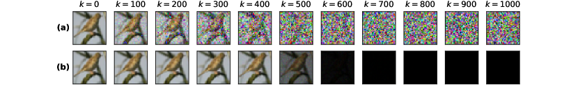
Figure 5: Figure 1 without an adjusted colormap.

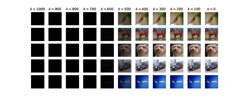
Figure 6: Figure 3 without an adjusted colormap.

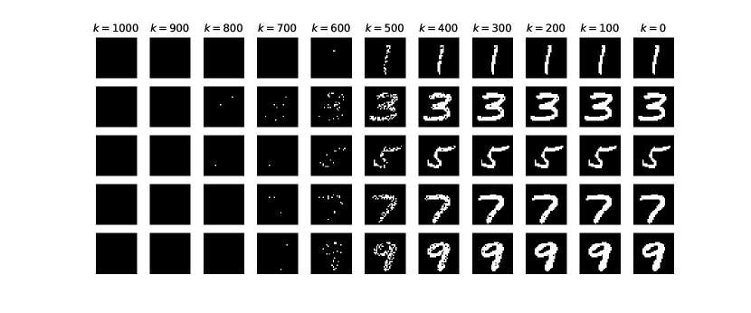
Figure 11: Generation of binarized MNIST samples.

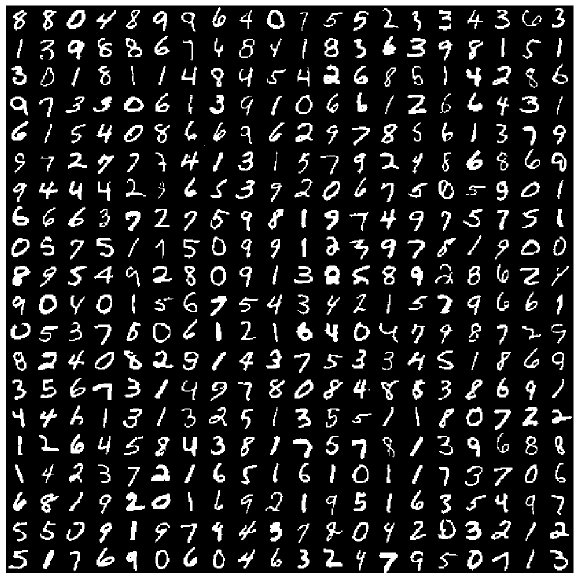
Figure 12: Four hundred binarized MNIST samples generated by Blackout Diffusion.

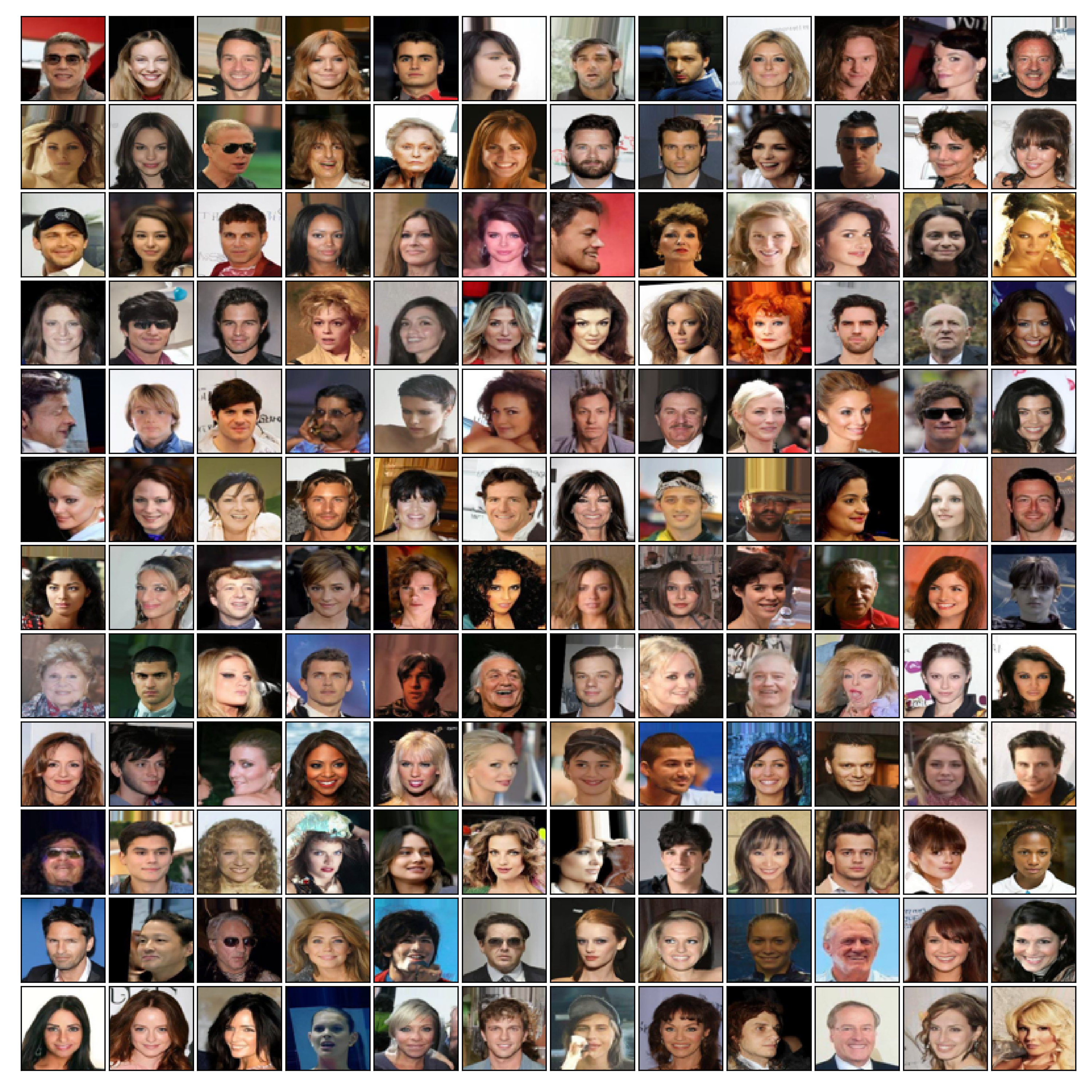
Figure 13: 144 samples generated by Blackout Diffusion trained on the Celeb-A dataset by the instantaneous loss function Eq. (14) and generated by $\tau$-leaping (Poisson random number) during inference (FID=3.22).

References

- Abate & Whitt (1987) Abate, J. and Whitt, W. Transient behavior of the M/M/l queue: Starting at the origin. Queueing Systems, 2(1):41–65, March 1987. ISSN 1572-9443. doi: 10.1007/BF01182933.
- Anderson (1982) Anderson, B. D. Reverse-time diffusion equation models. Stochastic Processes and their Applications, 12(3):313–326, 1982. ISSN 0304-4149. doi: https://doi.org/10.1016/0304-4149(82)90051-5.
- Austin et al. (2021) Austin, J., Johnson, D. D., Ho, J., Tarlow, D., and van den Berg, R. Structured denoising diffusion models in discrete state-spaces. In Ranzato, M., Beygelzimer, A., Dauphin, Y. N., Liang, P., and Vaughan, J. W. (eds.), Advances in Neural Information Processing Systems 34: Annual Conference on Neural Information Processing Systems 2021, NeurIPS 2021, December 6-14, 2021, virtual, pp. 17981–17993, 2021.
- Bansal et al. (2022) Bansal, A., Borgnia, E., Chu, H.-M., Li, J. S., Kazemi, H., Huang, F., Goldblum, M., Geiping, J., and Goldstein, T. Cold diffusion: Inverting arbitrary image transforms without noise, 2022.
- Campbell et al. (2022) Campbell, A., Benton, J., De Bortoli, V., Rainforth, T., Deligiannidis, G., and Doucet, A. A continuous time framework for discrete denoising models. In Koyejo, S., Mohamed, S., Agarwal, A., Belgrave, D., Cho, K., and Oh, A. (eds.), Advances in Neural Information Processing Systems, volume 35, pp. 28266–28279. Curran Associates, Inc., 2022.
- De Bortoli et al. (2021) De Bortoli, V., Thornton, J., Heng, J., and Doucet, A. Diffusion schrödinger bridge with applications to score-based generative modeling. In Ranzato, M., Beygelzimer, A., Dauphin, Y., Liang, P., and Vaughan, J. W. (eds.), Advances in Neural Information Processing Systems, volume 34, pp. 17695–17709. Curran Associates, Inc., 2021.
- Faggionato et al. (2009) Faggionato, A., Gabrielli, D., and Crivellari, M. R. Non-equilibrium thermodynamics of piecewise deterministic markov processes. Journal of Statistical Physics, 137(2):259–304, 2009. ISSN 00224715. doi: 10.1007/s10955-009-9850-x.
- Feller (1949) Feller, W. On the Theory of Stochastic Processes, with Particular Reference to Applications, pp. 403–432. 1949.
- Feller (1951) Feller, W. Two Singular Diffusion Problems. Annals of Mathematics, 54(1):173–182, 1951.
- Feller (1952) Feller, W. The parabolic differential equations and the associated semi-groups of transformations. Annals of Mathematics, 55(3):468–519, 1952.
- Gardiner (2009) Gardiner, C. W. Stochastic Methods: A Handbook for the Natural and Social Sciences. Number 13 in Springer Series in Synergetics. Springer, Berlin Heidelberg, 4th ed edition, 2009. ISBN 978-3-642-08962-6 978-3-540-70712-7.
- Gaudreault et al. (2018) Gaudreault, S., Rainwater, G., and Tokman, M. Kiops: A fast adaptive krylov subspace solver for exponential integrators. Journal of Computational Physics, 372:236–255, 2018. doi: https://doi.org/10.1016/j.jcp.2018.06.026.
- Gillespie (2001) Gillespie, D. T. Approximate accelerated stochastic simulation of chemically reacting systems. The Journal of Chemical Physics, 115(4):1716–1733, 2001. doi: https://doi.org/10.1063/1.1378322.
- Gilmer et al. (2017) Gilmer, J., Schoenholz, S. S., Riley, P. F., Vinyals, O., and Dahl, G. E. Neural message passing for quantum chemistry. In Precup, D. and Teh, Y. W. (eds.), Proceedings of the 34th International Conference on Machine Learning, volume 70 of Proceedings of Machine Learning Research, pp. 1263–1272. PMLR, 06–11 Aug 2017.
- Gong et al. (2022) Gong, S., Li, M., Feng, J., Wu, Z., and Kong, L. Diffuseq: Sequence to sequence text generation with diffusion models. 2022. doi: 10.48550/arxiv.2210.08933.
- Ho et al. (2020) Ho, J., Jain, A., and Abbeel, P. Denoising diffusion probabilistic models. In Larochelle, H., Ranzato, M., Hadsell, R., Balcan, M., and Lin, H. (eds.), Advances in Neural Information Processing Systems, volume 33, pp. 6840–6851. Curran Associates, Inc., 2020.
- Ho et al. (2022) Ho, J., Salimans, T., Gritsenko, A., Chan, W., Norouzi, M., and Fleet, D. J. Video diffusion models. 2022. doi: 10.48550/arxiv.2204.03458.
- Hoogeboom et al. (2021) Hoogeboom, E., Nielsen, D., Jaini, P., Forré, P., and Welling, M. Argmax flows and multinomial diffusion: Learning categorical distributions. In Ranzato, M., Beygelzimer, A., Dauphin, Y., Liang, P., and Vaughan, J. W. (eds.), Advances in Neural Information Processing Systems, volume 34, pp. 12454–12465. Curran Associates, Inc., 2021.
- Höppe et al. (2022) Höppe, T., Mehrjou, A., Bauer, S., Nielsen, D., and Dittadi, A. Diffusion models for video prediction and infilling. Transactions on Machine Learning Research, 2022.
- Huang et al. (2014) Huang, G.-R., Saakian, D. B., Rozanova, O., Yu, J.-L., and Hu, C.-K. Exact solution of master equation with gaussian and compound poisson noises. Journal of Statistical Mechanics: Theory and Experiment, 2014(11):P11033, nov 2014. doi: 10.1088/1742-5468/2014/11/P11033.
- Ingraham et al. (2019) Ingraham, J., Garg, V., Barzilay, R., and Jaakkola, T. Generative models for graph-based protein design. Advances in neural information processing systems, 32, 2019.
- Jiang et al. (2021) Jiang, D., Hsieh, C.-Y., Wu, Z., Kang, Y., Wang, J., Wang, E., Liao, B., Shen, C., Xu, L., Wu, J., et al. Interactiongraphnet: A novel and efficient deep graph representation learning framework for accurate protein–ligand interaction predictions. Journal of medicinal chemistry, 64(24):18209–18232, 2021.
- Karras et al. (2022) Karras, T., Aittala, M., Aila, T., and Laine, S. Elucidating the design space of diffusion-based generative models. 2022. doi: 10.48550/arxiv.2206.00364.
- Kim et al. (2022) Kim, D., Kim, Y., Kwon, S. J., Kang, W., and Moon, I.-C. Refining generative process with discriminator guidance in score-based diffusion models. 11 2022. URL \urlhttps://arxiv.org/abs/2211.17091v3.
- Kingma & Welling (2014) Kingma, D. P. and Welling, M. Auto-encoding variational bayes. 2nd International Conference on Learning Representations, ICLR 2014 - Conference Track Proceedings, (Ml):1–14, 2014.
- Kloeden & Platen (1999) Kloeden, P. E. and Platen, E. Numerical Solution of Stochastic Differential Equations. Number 23 in Applications of Mathematics. Springer, Berlin ; New York, corr. 3rd print edition, 1999. ISBN 978-3-540-54062-5.
- Kolmogorov (1931) Kolmogorov, A. über die analytischen Methoden in der Wahrscheinlichkeitsrechnung. Mathematische Annalen, 104(1):415–458, December 1931. ISSN 1432-1807. doi: 10.1007/BF01457949.
- Kong et al. (2021) Kong, Z., Ping, W., Huang, J., Zhao, K., and Catanzaro, B. Diffwave: A versatile diffusion model for audio synthesis. In International Conference on Learning Representations, 2021.
- Li et al. (2016) Li, Q., Luo, K. H., Kang, Q., He, Y., Chen, Q., and Liu, Q. Lattice boltzmann methods for multiphase flow and phase-change heat transfer. Progress in Energy and Combustion Science, 52:62–105, 2016.
- Mao & Yuan (2006) Mao, X. and Yuan, C. Stochastic Differential Equations with Markovian Switching. Imperial college press, 2006. doi: 10.1142/p473.
- Munsky et al. (2015) Munsky, B., Fox, Z., and Neuert, G. Integrating single-molecule experiments and discrete stochastic models to understand heterogeneous gene transcription dynamics. Methods, 85:12–21, 2015.
- Nichol & Dhariwal (2021) Nichol, A. Q. and Dhariwal, P. Improved denoising diffusion probabilistic models. In Meila, M. and Zhang, T. (eds.), Proceedings of the 38th International Conference on Machine Learning, volume 139 of Proceedings of Machine Learning Research, pp. 8162–8171. PMLR, 18–24 Jul 2021.
- Pawula (1967) Pawula, R. F. Approximation of the linear boltzmann equation by the fokker-planck equation. Phys. Rev., 162:186–188, Oct 1967. doi: 10.1103/PhysRev.162.186.
- Pichon et al. (2018) Pichon, X., Lagha, M., Mueller, F., and Bertrand, E. A growing toolbox to image gene expression in single cells: Sensitive approaches for demanding challenges. Molecular Cell, 71(3):468–480, 2018. ISSN 1097-2765. doi: 10.1016/j.molcel.2018.07.022.
- Revuz & Yor (1994) Revuz, D. and Yor, M. Continuous Martingales and Brownian Motion. Number 293 in Grundlehren Der Mathematischen Wissenschaften. Springer-Verlag, Berlin ; New York, 2nd ed edition, 1994. ISBN 978-3-540-57622-8 978-0-387-57622-0.
- Rezende & Mohamed (2015) Rezende, D. and Mohamed, S. Variational inference with normalizing flows. In International conference on machine learning, pp. 1530–1538. PMLR, 2015.
- Rombach et al. (2022) Rombach, R., Blattmann, A., Lorenz, D., Esser, P., and Ommer, B. High-resolution image synthesis with latent diffusion models. In Proceedings of the IEEE/CVF Conference on Computer Vision and Pattern Recognition, pp. 10684–10695, 2022.
- Saad (1992) Saad, Y. Analysis of some krylov subspace approximations to the matrix exponential operator. SIAM Journal on Numerical Analysis, 29(1):209–228, 1992. doi: https://doi.org/10.1137/0729014.
- Smith et al. (2018) Smith, J. S., Roitberg, A. E., and Isayev, O. Transforming computational drug discovery with machine learning and ai. ACS Medicinal Chemistry Letters, 9(11):1065–1069, 2018. doi: https://doi.org/10.1021/acsmedchemlett.8b00437.
- Sohl-Dickstein et al. (2015) Sohl-Dickstein, J., Weiss, E. A., Maheswaranathan, N., and Ganguli, S. Deep Unsupervised Learning using Nonequilibrium Thermodynamics, November 2015.
- Song et al. (2021a) Song, J., Meng, C., and Ermon, S. Denoising diffusion implicit models. In International Conference on Learning Representations, 2021a.
- Song & Ermon (2019) Song, Y. and Ermon, S. Generative modeling by estimating gradients of the data distribution. In Advances in Neural Information Processing Systems, pp. 11895–11907, 2019.
- Song & Ermon (2020) Song, Y. and Ermon, S. Improved Techniques for Training Score-Based Generative Models, October 2020.
- Song et al. (2021b) Song, Y., Durkan, C., Murray, I., and Ermon, S. Maximum Likelihood Training of Score-Based Diffusion Models, October 2021b.
- Song et al. (2021c) Song, Y., Sohl-Dickstein, J., Kingma, D. P., Kumar, A., Ermon, S., and Poole, B. Github repository of score-Based Generative Modeling through Stochastic Differential Equations. \urlhttps://github.com/yang-song/score_sde_pytorch, February 2021c. [Online; accessed 17-Jan-2023].
- Song et al. (2021d) Song, Y., Sohl-Dickstein, J., Kingma, D. P., Kumar, A., Ermon, S., and Poole, B. Score-Based Generative Modeling through Stochastic Differential Equations, February 2021d.
- van Kampen (2007) van Kampen, N. G. Stochastic Processes in Physics and Chemistry. Elsevier Science B.V., Amsterdam, 2007.
- Vargas et al. (2021) Vargas, F., Thodoroff, P., Lamacraft, A., and Lawrence, N. D. Solving schrödinger bridges via maximum likelihood. Entropy, 23(9):1134, 2021. doi: 10.3390/e23091134.
- Vargas et al. (2023) Vargas, F., Ovsianas, A., Fernandes, D., Girolami, M., Lawrence, N. D., and Nüsken, N. Bayesian learning via neural schrödinger-föllmer flows. Stat. Comput., 33(1):3, 2023. doi: 10.1007/s11222-022-10172-5.
- Weber & Frey (2017) Weber, M. F. and Frey, E. Master equations and the theory of stochastic path integrals. Reports on Progress in Physics, 80(4), 2017. ISSN 00344885. doi: 10.1088/1361-6633/aa5ae2.
- Wieder et al. (2020) Wieder, O., Kohlbacher, S., Kuenemann, M., Garon, A., Ducrot, P., Seidel, T., and Langer, T. A compact review of molecular property prediction with graph neural networks. Drug Discovery Today: Technologies, 37:1–12, 2020. ISSN 1740-6749. doi: https://doi.org/10.1016/j.ddtec.2020.11.009.
- Ye et al. (2022) Ye, M., Wu, L., and Liu, Q. First hitting diffusion models for generating manifold, graph and categorical data. In Koyejo, S., Mohamed, S., Agarwal, A., Belgrave, D., Cho, K., and Oh, A. (eds.), Advances in Neural Information Processing Systems, volume 35, pp. 27280–27292. Curran Associates, Inc., 2022.
- Zhang & Chen (2022) Zhang, Q. and Chen, Y. Path integral sampler: A stochastic control approach for sampling. In The Tenth International Conference on Learning Representations, ICLR 2022, Virtual Event, April 25-29, 2022. OpenReview.net, 2022.
- Zhou et al. (2020) Zhou, J., Cui, G., Hu, S., Zhang, Z., Yang, C., Liu, Z., Wang, L., Li, C., and Sun, M. Graph neural networks: A review of methods and applications. AI Open, 1:57–81, 2020.