Lightweight Online Learning for Sets of Related Problems in Automated Reasoning

Abstract

We present Self-Driven Strategy Learning (sdsl), a lightweight online learning methodology for automated reasoning tasks that involve solving a set of related problems. sdsl does not require offline training, but instead automatically constructs a dataset while solving earlier problems. It fits a machine learning model to this data which is then used to adjust the solving strategy for later problems. We formally define the approach as a set of abstract transition rules. We describe a concrete instance of the sdsl calculus which uses conditional sampling for generating data and random forests as the underlying machine learning model. We implement the approach on top of the kissat solver and show that the combination of kissat+sdsl certifies larger bounds and finds more counter-examples than other state-of-the-art bounded model checking approaches on benchmarks obtained from the latest Hardware Model Checking Competition.

I Introduction

Many automated reasoning tasks involve solving a set of related problems that share common structure. For example, in Bounded Model Checking [1, 2], one repeatedly checks deeper and deeper unrolls of a transition system for a property violation. In iterative (e.g., counter-example-guided) abstraction refinement [3], one verifies a condition on an increasingly precise model of a system. And in symbolic execution [4], one analyzes the possible outcomes of a program on symbolic inputs by incrementally adding path conditions. Often, a fixed, predetermined high-level solving strategy (e.g., the choice of a solver and its parameter settings) is used in this iterative solving process. However, given the structural similarity within the set of problems, a natural question is: can we leverage information gathered while solving earlier problems to adjust the solving strategy for later problems on the fly?

Adapting high-level solving strategies for particular problem distributions, a practice often termed meta-algorithmic design [5], is already a well-established technique. Automated configuration techniques [6], which optimize an algorithm’s performance on a given set of problems, are widely used among practitioners. Per-instance algorithm selection techniques (e.g., SATzilla [7]) train machine learning models to predict a suitable strategy for a given problem based on its structural characteristics. More recently, attempts to improve constraint solving using deep learning also generally follow the paradigm of choosing a particular problem distribution (which can be either broad, such as main-track benchmarks from SAT competitions [8], or narrow, such as graph coloring problems [9]), gathering training data using instances in that distribution, and learning a strategy over the data.

A shared, and arguably undesirable,trait of the aforementioned approaches is that they all involve an offline phase, in which significant time and (often manual) effort are required to obtain an optimized solving strategy that can be used on new unseen problems. While the cost of the offline phase might be justified by the potential performance gain in the long run, the very distinction between an offline phase and an online phase already makes the reasoning less automated.

Our first observation is that for an automated reasoning procedure whose execution involves solving a set $S$ of related problems, it is possible to move the meta-algorithmic design online, as part of the solving, by narrowing the scope of problem distribution all the way down to $S$ itself. More concretely, we propose to solve some of the problems in $S$ not just once, but multiple times, each time using a different solving strategy from a space of candidates. The strategies used for solving later problems are selected based on information recorded during the multiple runs (e.g., using lightweight machine learning techniques). We present this general method, which we term Self-Driven Strategy Learning (sdsl), as a set of transition rules, which can be used to model different ways of carrying out on-the-fly meta-algorithmic design.

Though there are many possible ways to instantiate sdsl, we focus on a strategy space consisting of one fixed solver whose parameters are allowed to vary. One obvious method for exploring this strategy space involves choosing the first few problems, optimizing the parameter settings for them with a standard tuning procedure, and then using the optimized strategy for future problems. However, a drawback of this approach is that it only operates on a fixed set of problems and cannot explicitly take into account possible relationships between this set of problems and later problem instances.

To allow for such flexibility, our second observation is that a tuning procedure can be viewed, not as a way to select a specific solving strategy, but instead as a means of creating a dataset, where each data point is a pair consisting of a particular solving strategy and a particular problem in the problem set. A machine learning model is trained on this dataset to predict the effect of a given solving strategy on a given problem. The model can then be used as an oracle to select the solving strategy for future problems.

Figure 1: Executions of Bounded Model Checking with and without sdsl on a hardware model checking benchmark (arb.n2.w128.d64). The trajectories show the cumulative wall-clock time required to certify a bound.

We apply our methodology to a case study of Bounded Model Checking (BMC) problems. We study different sdsl instantiations and compare against existing model checkers. On satisfiable and unsolved bitvector benchmarks from the latest Hardware Model Checking Competition [10], our approach consistently boosts the performance of a BMC-procedure built on top of the kissat SAT solver [11]. Additionally, it compares favorably against state-of-the-art open-source model checkers avr [12] and pono [13], contributing several unique solutions and speeding up many more. A preview on a single benchmark is shown in Fig. 1. We see that sdsl invests time learning a good solving strategy in the beginning, which results in better performance when solving later problems.

We summarize our main contributions as follows:

1. we propose to move meta-algorithmic design online as part of solving a set of related problems;

2. we propose a general methodology called Self-Driven Strategy Learning and present it formally as a set of transition rules; and

3. we implement our approach and apply it to Bounded Model Checking problems, where it shows significant improvement over other state-of-the-art approaches.

The rest of the paper is organized as follows. After a discussion of related work in Sec. II, we first define a basic calculus for iteratively solving a set of related problems in Sec. III. Next, sdsl is presented as an extension of this calculus with additional rules for data collection, learning, and strategy updates in Sec. IV. We explore the design space of sdsl in Sec. V, discussing how to sample training data and which machine learning models to use. In Sec. VI, we describe in detail the instantiation of sdsl for Bounded Model Checking. In Sec. VII we present experimental results on Bounded Model Checking problems, and finally, we conclude with an account of current limitations and future directions in Sec. VIII.

II Related Work

Our approach is inspired and informed by several existing lines of work.

Incremental solving

A well-established paradigm for exploiting structural similarity is incremental solving [14] in which each new query to a solver can be made by modifying the most recent formulas asserted in the previous query without resetting the solver. sdsl is an orthogonal approach for leveraging structural similarity and may be preferable in cases where incremental solving is not beneficial or not supported.

In principle, the two can be combined. A straightforward way would be to switch to incremental solving mode after fixing a solving strategy. A tighter combination would require updating strategies between incremental invocations, something that current solvers typically do not allow. In case one wants to both switch solvers on the fly and leverage incrementality, proof-transfer techniques such as solver state migration [15] are likely needed. For our particular BMC case study, we found that the direct use of an incremental SAT/SMT solver has mixed effects on performance (see App. D). This suggests that it might be worth revisiting BMC-specific incremental solving techniques such as conflict clause shifting [16] before investigating the interplay between sdsl and incremental solving in BMC, which we leave for future work.

Automated Configuration

Our work is motivated by the success of offline meta-algorithmic design approaches such as automated configuration [17, 6, 18] and per-instance algorithm selection [7, 19, 20]. Automated configuration focuses on finding (near) optimal parameter settings of an algorithm for a fixed set of problems, using either local search or performance prediction techniques [21, 22, 23]. Per-instance algorithm selection techniques were among the first to utilize machine learning to improve constraint solving. The idea is to train an oracle to predict the performance (e.g., runtime) of a set of candidate algorithms on a formula based on its structural characteristics. sdsl differs from both approaches primarily in that it moves meta-algorithmic design online.

ML for AR

Machine Learning has been applied in multiple ways to expedite a variety of automated reasoning tasks, including satisfiability checking [8, 9, 24, 25, 26, 27, 28, 29, 30], Mixed-Integer Convex Programming [31, 32], program/function synthesis [33, 34, 35], and symbolic execution [36, 37].

While most existing techniques require an offline training phase, the general idea of using online learning also appears in previous work. The Conflict-Driven Clause Learning paradigm itself can be viewed as online learning. In the MapleSAT solver [26, 27], branching is formulated as a multi-armed bandit problem where the estimated reward of each arm (i.e., variable) is maintained and updated throughout the solving. This reinforcement learning interpretation of a dynamic branching heuristic is perhaps inspired by the study [38] of the popular VSIDS [39] branching heuristic and its later variants [40], which also track a score for each variable during the solving. In contrast to this direction of online learning, sdsl operates on a set of related problems rather than on a single instance. Moreover, sdsl focuses on selecting from a set of existing strategies rather than inventing new ones.

To conclude this section, we remark that in practice, offline learning, “in-solver” online learning, and sdsl could be combined to solve a set of related problems. For example, one could choose to use SAT/SMT solvers with built-in learning components, set the initial solving strategy using offline learning, and then use sdsl to further customize the strategy online. The exploration of such combinations is beyond the scope of this paper, but is a promising future direction.

III Solving Sets of Related Problems

In this section, we present a simple calculus, SR, for iteratively solving a set of related problems. Let $\mathcal{F}=\{f_{1},\dots,f_{\mathbf{K}}\}$ be a set of $\mathbf{K}$ related formulas. Assume we have a function $\mathbf{check}:\mathcal{F}\times\mathcal{V}\rightarrow\{\textsc{sat},\textsc{unsat}\}$, which takes as input a formula $f\in\mathcal{F}$ and a solving strategy $v$ (from a set $\mathcal{V}$ called the strategy space) and returns either sat (satisfiable) or unsat (unsatisfiable). Additionally, assume that we can stop once any formula is sat.

The rules of the basic SR calculus are shown in Fig. 2. The rules operate over a configuration, which is either one of the distinguished symbols $\{\textsc{success},\textsc{fail}\}$ or a tuple $\langle i,v\rangle$, where $i\in[1,\mathbf{K}]$ is the current formula index and $v\in\mathcal{V}$ is the current solving strategy. The rules describe the conditions under which a certain configuration can transform into another configuration. The Next rule says that if the current formula is unsatisfiable and the maximal index $\mathbf{K}$ has not been reached yet, then the current index will be increased. On the other hand, if the current formula is unsatisfiable and it is the last formula, the Failure rule transitions the system to the fail configuration. The Success rule states that success can be reached when the current formula is satisfiable.

  $i<\mathbf{K}\quad\mathbf{check}(f_{i},v)=\textsc{unsat}$    (Next)           $i,v\Longrightarrow i+1,v$

  $i=\mathbf{K}\quad\mathbf{check}(f_{i},v)=\textsc{unsat}$    (Failure)              $i,v\Longrightarrow\textsc{fail}$

  $\mathbf{check}(f_{i},v)=\textsc{sat}$    (Success)      $i,v\Longrightarrow\textsc{success}$

Figure 2: Transition rules for solving a set of related problems. The starting configuration is $\langle 1,v\rangle$.

An SR-execution is a sequence of configurations that respect the rules in SR. Note that no rule updates the solving strategy $v$. We augment the calculus with strategy updates next.

Given two configurations $C,C^{\prime}$, we use $C\vdash C^{\prime}$ to denote $C$ can transition (in one or more steps) to $C^{\prime}$. We state the following two propositions which are straightforward to verify.

Proposition 1 (Soundness and Completeness)

$\mathcal{F}$ contains a satisfiable formula if and only if $\langle 1,v\rangle\vdash\textsc{success}$.

Proposition 2 (Termination)

There exist no infinite SR-executions.

IV Self-Driven Strategy Learning

      $v_{\text{s}}\in\mathcal{V}\quad j\leq i\quad c=\mathbf{cost}(f_{j},v_{\text{s}})$    (Collect)    $i,v,D,T\Longrightarrow i,v,D\cup\{\langle v_{\text{s}},j,c\rangle\},T$

          $T^{\prime}=\mathbf{fit}(D)$    (Train)    $i,v,D,T\Longrightarrow i,v,D,T^{\prime}$

   $\mathcal{V}_{\text{s}}\subseteq\mathcal{V}\quad v^{\prime}=\operatorname*{arg\,min}_{v_{\text{s}}\in\mathcal{V}_{\text{s}}}T(v_{\text{s}},i)$    (Strategize)          $i,v,D,T\Longrightarrow i,v^{\prime},D,T$

Figure 3: Additional transition rules for Self-Driven Strategy Learning.

IV-A Informal Presentation

Self-Driven Strategy Learning (sdsl) attempts to learn, on the fly, which solving strategy among a set of candidates $\mathcal{V}$ to use for each formula in $\mathcal{F}$. Learning is based on data gathered during solving. To obtain the data, we occasionally solve a formula multiple times, each time with a different strategy in $\mathcal{V}$. For a strategy $v_{\text{s}}$, we record its effect, $c\in\mathbb{R}$, when solving $f_{i}$ by creating a data point $\langle v_{\text{s}},i,c\rangle$, where $c$ is a measure of the cost of the strategy. For example, $c$ could be the total run time required to solve $f_{i}$.

Given such a dataset, an oracle $T:\mathcal{V}\times[1,\mathbf{K}]\mapsto\mathbb{R}$ is trained to predict the cost of a given strategy when run on a given formula. When solving a new formula, we select the one that $T$ predicts will be most effective, and as more data is collected with each call to $\mathbf{check}$, $T$ is updated.

An essential characteristic of sdsl is that the training data is gathered for a specific, and a priori unknown, set of formulas in an online and automatic manner, as part of the solving process. This approach has two challenging implications. The learning process must not incur a large overhead; otherwise, insufficient time is left for actual solving. Additionally, the choice of $\mathcal{V}$ is crucial as it must be large enough to contain good candidate strategies but also not too large to explore. We address these challenges in Sections V and VI, respectively.

IV-B Formal presentation

Formally, we present sdsl as an extension of SR. Configurations are as in SR except that tuple configurations $\langle i,v,D,T\rangle$ have two additional components (assumed to be left unchanged by rules in SR): $D\in\mathcal{P}(\mathcal{V}\times[1,\mathbf{K}]\times\mathbb{R})$ is a dataset, each of whose members records the result of running a single strategy on a single formula; and $T:\mathcal{V}\times[1,\mathbf{K}]\mapsto\mathbb{R}$ is an oracle (e.g., a machine learning model) that predicts the cost of a strategy on a formula. Initially, $D$ is empty, and $T$ is arbitrary (e.g., always return 0). The additional transition rules of sdsl are described in Fig. 3.

The Collect rule samples a strategy $v_{\text{s}}\in\mathcal{V}$, evaluates its cost when solving $f_{j}$, and augments $D$ with this new data. The rule is parameterized by a function $\mathbf{cost}:\mathcal{F}\times\mathcal{V}\mapsto\mathbb{R}$. The Train rule updates the oracle $T$ with a new one trained on the current dataset $D$. It is parameterized by a machine learning algorithm $\mathbf{fit}$ (e.g., k-NN, tree ensemble, deep learning, etc.). Finally, the Strategize rule updates the current strategy by sampling a set of strategies $\mathcal{V}_{\text{s}}$ from $\mathcal{V}$ and choosing the one with the best predicted cost for the current index $i$. The extended calculus is still sound and complete (i.e., Proposition 1 still holds). Since the added rules can effectively be applied at any time, Proposition 2 only holds if we allow only a finite number of applications of the new rules.

Note that in the Collect rule, the results of solving the formula $f_{j}$ are discarded, as $f_{j}$ must have been solved already in some previous application of the Next rule. It is possible to extend the SR calculus to allow unknown results from $\mathbf{check}$, but the completeness property would be lost.

A reasonable strategy for applying sdsl rules is as follows:

1. After every application of Next, issue one learning epoch; that is, apply Collect $m$ times on the current problem, then apply Train;

2. If Train has been applied at least once, apply Strategize whenever $i$ is updated;

3. If the estimated learning time exceeds some threshold $n$, override the first policy and do not issue any more learning epochs;

4. Terminate whenever Success or Failure applies.

The estimated learning time is calculated as the time spent on learning so far plus $m\cdot t$, where $t$ is the runtime of solving the current problem using the current strategy. If $|\mathcal{V}|$ is small, it may be reasonable to use $m=|\mathcal{V}|$ and try each strategy from $\mathcal{V}$. In the more general scenario where $m\ll|\mathcal{V}|$, the choice of which samples to use impacts the quality of the dataset. We discuss this choice and present a conditional sampling procedure in Sec. V-A. The purpose of restricting the training time in step three is to ensure that training does not dominate the total time taken. This simple criterion for when to stop learning already works reasonably well in practice. We leave the exploration of more sophisticated heuristics to future work.

V Design Space in sdsl

This section discusses the design space in the implementation of sdsl and proposes solutions to the following questions: 1) How should training data be sampled? 2) Which machine learning model and training algorithm should be used? The solutions we propose focus on the case where a strategy is simply a set of values for a specific set of solver parameters. In this case, the strategy space is the cartesian product of $p$ sub-strategy spaces, each representing a single parameter: $\mathcal{V}=\mathcal{V}_{1}\times\ldots\times\mathcal{V}_{p}$. The set of possible values for each parameter can vary (e.g., parameter values could be Booleans, strings, or numbers), but for now we assume each $\mathcal{V}_{i}$ is finite.

V-A Gathering Informative Training Data

To make the most informed decision, we could try all candidate strategies on all previously considered problems, but this is infeasible when $|\mathcal{V}|$ is large. In the following, we consider the scenario where $m$ samples are drawn from a strategy space $\mathcal{V}$, where $m\ll|\mathcal{V}|$.

In this restrictive setting, we need to ensure our dataset contains a sufficient number of low-cost strategies (if there are any). Sampling uniformly is unlikely to achieve this goal because in practice, many or most candidate strategies could have high cost. For this reason, we propose to explicitly favor low-cost strategies in the sampling process. One way to do this is by using Markov-Chain Monte-Carlo (MCMC) sampling, which in our setting can be used to generate a sequence of solving strategies with the desirable property that in the limit, strategies with the lowest cost are most frequently drawn. A popular MCMC method is the Metropolis-Hastings (M-H) Algorithm [41], instantiated in the context of sdsl as follows:

1. Choose a current strategy $v$;

2. Propose to replace the current strategy with a new one $v^{\prime}$, which comes from a proposal distribution $q(v^{\prime}|v)$;

3. If $\mathbf{cost}(f,v^{\prime})\leq\mathbf{cost}(f,v)$, accept $v^{\prime}$ as the current strategy;

4. Otherwise, accept $v^{\prime}$ as the current strategy with some probability $a(v{\rightarrow}v^{\prime})$ (e.g., a probability inversely proportional to the increase in cost);

5. Go to step 2.

This process is repeated until $m$ samples are drawn. Importantly, under this scheme, a proposal that results in lower cost is always accepted, while a proposal that does not may still be accepted. This means that the algorithm greedily moves to a better strategy whenever possible, but also has a means for escaping local minima. In our implementation, the acceptance probability is computed using a common method [42] described as follows. We first transform $\mathbf{cost}(f,v)$ into a probability distribution $p(v)$:

$$p(v)\propto\exp(-\beta\cdot\mathbf{cost}(f,v))\enspace,$$

where $\beta>0$ is a configurable parameter. The acceptance probability is then computed as:

$$a(v{\rightarrow}v^{\prime}) =\min\left(1,\frac{p\left(v^{\prime}\right)}{p\left(v\right)}\right)$$

$$=\min\left(1,\exp\left(\beta\cdot\left(c-c^{\prime}\right)\right)\right)\enspace,$$

where $c=\mathbf{cost}(f,v)$ and $c^{\prime}=\mathbf{cost}(f,v^{\prime})$. Under this acceptance probability, the larger that $c^{\prime}$ is compared to $c$, the lower the probability to accept. On the other hand, the larger $\beta$ is, the more reluctant we are to move to a worse proposal.

To ensure the aforementioned convergence property of MCMC in the limit, the proposal distribution must be both symmetric and ergodic. For discrete search spaces, a common proposal distribution is the symmetric random walk, which moves to one of the neighbors of the current sample with equal probability. For our strategy space, we define the neighbors of a strategy as all strategies for which exactly $k$ parameter values are different. We use $k=1$ in our implementation.

Note that MCMC sampling can be used not only in the data collection process, but also in the Strategize rule (i.e., to choose $\mathcal{V}_{\text{s}}\subseteq\mathcal{V}$). Since in this case we use the machine learning model as an oracle of $\mathbf{cost}$ (which is much cheaper than calling a solver), a larger sample size is affordable.

The sampling scheme presented above largely coincides with many local search approaches used in the automated configuration literature [5]. Borrowing more insights from that literature and devising more sophisticated sampling schemes are interesting directions for future work.

V-B Lightweight Online Learning

In the online setting, the machine learning model must generalize from sparse data in limited time. This means the model needs to be both robust against outliers and efficient to train. Training a neural network from scratch, for example, is likely unsuitable, because it requires large amounts of data and, depending on the architecture, could be costly to train. On the other hand, lightweight ensemble models, which consist of a set of sub-models with different strengths and weaknesses, are well-suited for sdsl.

Our data is what is often called tabular data, that is, it can be represented as a table with rows and columns, where each row corresponds to a sample, and each column corresponds to a feature. When the strategy space consists of parameter settings, each sample has $p+2$ features: the $p$ parameters, the problem index, and the cost. Tree-based ensemble methods such as random forests are generally considered to be a good match for such data [43].

A random forest consists of a set of $B$ regression trees $\{f_{1},\ldots,f_{B}\}$. Each tree is trained independently by sampling data from the data set $D$. A regression tree makes a prediction by following a path from the root node to a leaf node, based on the values of the input features, and returning the cost associated with the leaf node (which generally is the average of the costs of the training points that map to that leaf node). The predictions of a random forest $f$ are computed by averaging the predictions of the individual trees in $f$.

A random forest is both efficient to train and efficient for prediction [44]. The time complexity of training a random forest with $B$ trees is $O(B\cdot m\cdot n\cdot\log m)$, where $m$ is the number of data points and $n$ is the number of input features. The inference time complexity for a random forest is $O(B\cdot n)$.

Many machine learning algorithms are themselves parameterized and the performance of the model depends on a good choice of the hyperparameters. For a tree-based algorithm like random forest, an important hyperparameter is the maximal depth allowed for each individual regression tree: too shallow, and the model’s prediction will be inaccurate; too deep, and the model might overfit to outliers. The standard way to find suitable values of the hyperparameters is via (cross-)validation: split the data into a training set and a validation set, train models with different hyperparameters on the training set, evaluate them on the validation set, and pick the best one. However, in the sdsl setting where data is already sparse, validation is less feasible because it is hard to make sure that both the training set and the validation set are representative of the input space. Instead, we propose the following pragmatic heuristic: start by training a random forest with shallow trees and then retrain with incrementally deeper trees as needed until the training score is high enough.

VI Case study: Bounded Model Checking

Bounded Model Checking (BMC) [1, 2, 16] is a well-known technique for checking whether a property $P$ holds along bounded executions of a given system $M$. The algorithm starts by checking all executions of length $k$; if no counter-example is found, $k$ is increased and the system checked until either a counter-example is found, the problem becomes intractable, or some upper bound on $k$ is exceeded.

BMC is useful in practice for at least two reasons. First, it is often the most efficient way to find counter-examples (if they exist) when trying to prove that a system has a particular property. Second, when techniques capable of providing a full (i.e. unbounded) proof fail (which is often the case in practice), BMC still establishes a certain confidence in the system by providing formal guarantees for bounded executions. The larger the certified bound, the stronger the guarantee.

A basic BMC formula for checking whether a property $P$ holds for a system $M$ along executions of length $k$ is:

$$I_{0}\land\bigwedge^{k-1}_{i=0}\rho(i,i+1)\land(\bigvee^{k}_{i=0}\neg P_{i})\enspace,$$

where $I_{0}$ represents the initial state of $M$, $\rho(i,i+1)$ represents how the system evolves in a single step, and $P_{i}$ represents the property at step $i$ in the execution. This formula is satisfiable iff there is an execution of length less than or equal to $k$ such that the property $P$ does not hold at the end of the execution.

In practice, when the bound is increased, additional constraints are added stating that previously checked states are safe (in order to prune the search space). For example, suppose the check for bound $k^{\prime}$ is unsatisfiable. To check bound $k>k^{\prime}$, we use the following formula:

$$bmc(k^{\prime},k):=I_{0}\land\bigwedge^{k-1}_{i=0}\rho(i,i+1)\land{\color[rgb]{1,0,0}\bigwedge^{k^{\prime}}_{i=0}P_{i}}\land(\bigvee^{k}_{{\color[rgb]{1,0,0}i=k^{\prime}+1}}\neg P_{i})\enspace.$$

We use BMC as a case study for our approach. For a given system and property, we solve the following set of problems:

$$\mathcal{F}=\{bmc(k-s,k)\ |\ k=i\cdot s,1\leq i\leq\mathbf{K}\}\enspace,$$

where $s$ is the step size. We focus on hardware model checking problems where the set of formulas to solve is in the theory of bitvectors [45]. We use standard techniques to encode the bitvector problems as Boolean satisfiability (SAT) problems [46]. Thus, $\mathcal{F}$ is a set of Boolean formulas, and we can implement $\mathbf{check}$ using an off-the-shelf SAT solver. We use the state-of-the-art kissat SAT solver [11].

In the following, we discuss the choice of the cost function $\mathbf{cost}$ and the strategy space $\mathcal{V}$ for this case study.

VI-A Choosing the Cost Function

One plausible cost function for a strategy $v$ and a formula $f_{i}$ is the ratio of the runtime to that of some default strategy $v_{0}$, i.e., if the runtime is $t$ with strategy $v$ and $t_{0}$ with $v_{0}$, then $\mathbf{cost}(f_{i},v)=\frac{t}{t_{0}}$. While this definition works in practice, the use of runtime makes sdsl’s behavior non-deterministic across different runs. This is undesirable for many reasons, including experimental reproducibility. Therefore, we instead use the number of conflicts generated by the SAT solver, which is accepted as a good proxy for runtime [47]. Given the same parameter settings, the number of conflicts generated by kissat on the same problem is deterministic.

VI-B Choosing the strategy space

As discussed in Sec. IV-B, the choice of the strategy space is crucial to the effectiveness of sdsl. kissat has over 90 configurable parameters, so considering all of them is impractical. One plausible approach is to rely on expert/domain knowledge and empirical studies to identify a reasonable set of parameters to consider. We follow this approach to define two strategy spaces for kissat.

The first one, $\mathcal{V}_{exp}$ (Table I), is based on a study by Dutertre [48] on the effect of SAT solver parameters on bitvector problems. We allow two possible values for each parameter, the default one and an alternative one. For options that were found to be beneficial in [48], we include the corresponding parameter in kissat and for non-Boolean parameters, we set the alternative value to be more aggressive; for Boolean parameters, we simply set the alternative value to be the opposite of the default. In total, $\mathcal{V}_{exp}$ contains $8192$ $(2^{13})$ possible parameter settings.

TABLE I: The strategy space $\mathcal{V}_{exp}$ based on  [48].

kissat option	default	alternative
and	1	0
bumpreasonsrate	10	1
chrono	1	0
eliminateint	500	50
eliminateocclim	2000	20
forwardeffort	100	200
ifthenelse	1	0
probeint	100	10
rephaseint	1000	100
stable	1	0
substituteeffort	10	20
subsumeocclim	1000	10
vivifyeffort	100	200

The second strategy space, $\mathcal{V}_{dev}$ (Tab. II), is based on suggestions made by the developer of kissat. It contains significantly fewer possible parameter settings (216).

TABLE II: The strategy space $\mathcal{V}_{dev}$.

kissat option	default	alternative(s)
chrono	1	0
phase	1	0
stable	1	0, 2
target	1	0, 2
tier1	2	1
tier2	6	3, 9

Designing principled ways to automatically construct the strategy space (e.g., using techniques for assessing parameter importance [50]) is an important direction for future work.

VI-C Implementation

We implemented an sdsl-based BMC procedure in Python3. Our prototype takes as input a model checking problem in the btor/btor2 format [51, 52] and can run BMC on that input with or without sdsl. We implemented sdsl following the strategy described in Sec. IV-B. The BMC step size and the maximal bound are also command-line arguments. Additional input arguments include:

1. $\mathcal{V}$: path to a csv file representation of the strategy space (e.g., Tabs. I and  II);

2. $n$: the time budget for the learning epochs (see Sec. IV-B), by default 15% of the total time limit;

3. $m$: the number of samples to draw per learning epoch, by default 100;

4. The number of samples to draw in the Strategize rule, by default 500;

5. The number of trees in the random forest, by default 50;

6. The initial tree depth, by default a third of the number of parameters in $\mathcal{V}$;

7. The random seed, by default 0.

The default values are used in all experiments unless otherwise specified.

The formula $bmc(k^{\prime},k)$ is generated online by first creating a bitvector formula using the pono Model Checker [13], then bit-blasting it into a SAT formula using the boolector solver [53]. The versions of the solvers are reported in App. A. Our prototype does not leverage incrementality for reasons discussed in Sec. II. We use the Scikit-Learn machine learning library [54] for training the Random Forest. Apart from the number of trees and the depth of the trees, we use the default hyperparameters of Scikit-Learn’s Random Forest module. The prototype runs on one thread, though the sampling, training, and inference are in principle parallelizable.

VII Experimental Evaluation

TABLE III: Evaluation of $\textsc{kissat + {sdsl}}_{\textit{exp}}$ on BV benchmarks of Hardware Model Checking Competition 2020 that were not solved during the competition. ep is the number of training epochs. $t_{\textit{learn}}$ is the time spent on data collection, training, and inference. $t_{\textit{c.s.}}$ is the cumulative time ($t_{\textit{learn}}$ included) to solve all the formulas up until the largest bound commonly solved by $\textsc{kissat + {sdsl}}_{\textit{exp}}$ and kissat. $k$ is the largest solved bound within 2 hours and is highlighted if a violation is found (i.e., the benchmark is solved).

	step size = 1							step size = 10
	$\textsc{kissat + {sdsl}}_{\textit{exp}}$				kissat		pono	$\textsc{kissat + {sdsl}}_{\textit{exp}}$				kissat		pono
Benchmark	ep	$t_{\textit{learn}}$	$t_{\textit{c.s.}}$	$k$	$t_{\textit{c.s.}}$	$k$	$k$	ep	$t_{\textit{learn}}$	$t_{\textit{c.s.}}$	$k$	$t_{\textit{c.s.}}$	$k$	$k$
arb.n2.w128.d64	10	1040	4816	59	7198	54	45	2	751	3676	70	4940	70	50
arb.n2.w64.d64	9	936	4431	59	6515	53	48	2	638	3985	70	4224	70	50
arb.n2.w8.d128	10	1031	5599	54	6795	52	45	2	1127	3932	60	5528	60	50
arb.n3.w16.d128	9	937	4898	58	7118	53	48	2	807	3653	70	5792	60	60
arb.n3.w64.d128	10	1062	4856	58	7132	53	44	1	84	3427	60	5120	60	50
arb.n3.w64.d64	10	985	4809	58	7055	53	46	2	919	3736	70	5018	70	50
arb.n3.w8.d128	9	983	4760	58	6996	53	46	2	906	3227	60	6017	60	50
arb.n4.w128.d64	9	963	6143	54	6107	53	46	2	1086	3704	70	5627	70	50
arb.n4.w16.d64	10	984	4768	57	6599	53	49	2	580	3349	70	5231	70	70
arb.n4.w8.d64	10	1081	5863	54	6659	52	48	2	617	3177	70	4563	70	50
arb.n5.w128.d64	9	1105	5095	57	6731	53	47	1	139	4204	70	5587	70	50
circ.w128.d128	7	845	5746	46	6549	44	39	1	536	2348	30	1743	30	20
circ.w128.d64	8	887	6071	47	6452	46	39	1	747	2688	30	1962	30	20
circ.w16.d128	11	967	4997	58	7179	54	47	2	876	5778	50	4978	50	40
circ.w64.d128	9	870	5409	51	6895	48	44	1	232	4575	40	4294	40	30
dspf.p22	4	1078	3741	31	5654	28	27	1	285	289	20	90	20	20
pgm.3.prop5	10	1019	7128	128	5663	133	131	2	618	6844	190	6052	190	170
picor.AX.nom.p2	2	929	3307	16	3636	15	14	1	117	279	20	151	20	20
picor.pcregs-p0	5	992	4020	32	6402	30	30	0	0	83	20	85	20	20
picor.pcregs-p2	5	840	6149	30	5003	31	31	0	0	89	20	91	20	20
shift.w128.d64	7	858	4098	27	5393	25	21	1	582	678	30	353	20	20
shift.w16.d128	9	1084	3020	45	5817	39	28	2	864	1731	50	2606	40	20
shift.w32.d128	8	821	2778	43	6273	35	27	1	216	2656	30	2424	30	20
zipversa.p03	5	1110	2961	82	6683	59	45	2	1182	2138	110	6622	90	330
Mean	8.1	975	4811	52.6	6354	48.7	43.1	1.5	580	2927	57.5	3712	55.4	55.4

We consider the bitvector track benchmarks from the latest Hardware Model Checking Competition (HWMCC) [10]. We omit all unsatisfiable benchmarks, since these are not solvable using BMC. What remain are 65 benchmarks that were reported to be satisfiable during the competition and 24 benchmarks that were unsolved during the competition. All experiments are performed on a cluster equipped with Intel(R) Xeon(R) CPU E5-2637 v4 @ 3.50GHz running Ubuntu 20.04. Each job is given one physical core and 8 GB memory.

VII-A Unrolling the unsolved benchmarks

In the first experiment, we focus on the 24 unsolved benchmarks. For each benchmark, the goal is to either find a property violation or to prove that the property holds for as large a bound as possible. A CPU time limit of 2 hours is given for each benchmark. We consider two BMC step sizes: 1 and 10. For each step size, we run as baselines our kissat-based BMC implementation without sdsl (denoted kissat) and the BMC engine of pono (denoted pono), which makes incremental calls to boolector to solve bitvector queries.

VII-A1 Performance of sdsl using the strategy space in Tab. I

We first evaluate $\textsc{kissat + {sdsl}}_{\textit{exp}}$, the sdsl-extended BMC procedure using $\mathcal{V}_{exp}$ (Tab. I) as the strategy space. The results are shown in Tab. III. We report the largest solved (i.e., certified or falsified) bound $k$ for each configuration. For $\textsc{kissat + {sdsl}}_{\textit{exp}}$ and kissat, we also show the total time to solve all formulas up until the largest commonly solved bound ($t_{\textit{c.s.}}$). For $\textsc{kissat + {sdsl}}_{\textit{exp}}$, this includes the time spent on learning. We further report the number of learning epochs (ep) and the time spent on learning ($t_{\textit{learn}}$) for $\textsc{kissat + {sdsl}}_{\textit{exp}}$. Graphic illustrations in the style of Fig. 1 and the duration of each training epoch are presented in App. E and App. F, respectively.

When the BMC step size is 1, $\textsc{kissat + {sdsl}}_{\textit{exp}}$ is able to certify larger bounds compared with the baseline configurations on 22 out of the 24 benchmarks, with an average bound increase of $3.9$ ($52.6-48.7$). This improvement is highly non-trivial, considering that to reach a larger bound, $\textsc{kissat + {sdsl}}_{\textit{exp}}$ needs to 1) certify all the formulas up to the baseline bound; 2) spend time (on average 975 seconds) learning a solving strategy; and 3) solve an additional set of harder formulas with the remaining time, one for each increase in the bound size. Comparing $t_{\textit{c.s.}}$ sheds further light on the performance gain enabled by sdsl: on average, $\textsc{kissat + {sdsl}}_{\textit{exp}}$ is $1.3\times$ faster ($\frac{6354}{4811}$) on the set of commonly solved problems. The fraction of $t_{\textit{c.s.}}$ that $\textsc{kissat + {sdsl}}_{\textit{exp}}$ spends on actual solving (not including learning) is $3836$ seconds ($4811-975$). Thus, on average a $1.7\times$ speedup ($\frac{6354}{3836}$) is achieved in the sheer performance of the SAT solver. Upon closer examination, the learning time is dominated by the data collection, with actual training and inference only taking 2.1% of $t_{\textit{learn}}$ on average.

When using BMC step size 10, both the kissat-based baseline and $\textsc{kissat + {sdsl}}_{\textit{exp}}$ find counter-examples on 8 benchmarks (highlighted in red). In all but one of those benchmarks, $\textsc{kissat + {sdsl}}_{\textit{exp}}$ finds counter-examples faster. Additionally, $\textsc{kissat + {sdsl}}_{\textit{exp}}$ certifies a larger bound than kissat on 4 benchmarks. For the remaining 12 benchmarks, the two configurations certify the same bounds, but $\textsc{kissat + {sdsl}}_{\textit{exp}}$ reduces the runtime on only 3 of them. One explanation for this is that the number of affordable learning epochs is significantly smaller when the step size is 10 due to the increased hardness of individual formulas. As a result, fewer strategies are considered. For example, on arb.n2.w128.d64, a total of 871 unique solving strategies are evaluated when the step size is 1, whereas only 175 strategies are evaluated when the step size is 10. Nonetheless, overall, $\textsc{kissat + {sdsl}}_{\textit{exp}}$ is still $1.3\times$ faster ($\frac{3712}{2927}$) at certifying the same bounds.

It is important to note that using step size 10 does not necessarily lead to a larger certified bound. Take circ.w128.d128 for example: $\textsc{kissat + {sdsl}}_{\textit{exp}}$ can unroll to an execution length of 46 with step size 1 while only unrolling to 30 with step size 10. This also applies to an incremental solver like pono, which certifies an execution length of 39 with step size 1 versus 20 with step size 10. This suggests that the optimal step size varies in practice.

TABLE IV: Evaluation of $\textsc{kissat + {sdsl}}_{\textit{dev}}$. The setup is the same as Tab. III

. step size = 1 step size = 10 $\textsc{kissat + {sdsl}}_{\textit{dev}}$ kissat $\textsc{kissat + {sdsl}}_{\textit{dev}}$ kissat Benchmark ep $t_{\textit{learn}}$ $t_{\textit{c.s.}}$ $k$ $t_{\textit{c.s.}}$ $k$ ep $t_{\textit{learn}}$ $t_{\textit{c.s.}}$ $k$ $t_{\textit{c.s.}}$ $k$ arb.n2.w128.d64 11 861 6714 54 7198 54 2 631 3720 70 4940 70 arb.n2.w64.d64 10 896 6158 54 6515 53 2 575 4981 70 4224 70 arb.n2.w8.d128 11 1006 6291 53 6795 52 2 684 3674 60 5528 60 arb.n3.w16.d128 9 824 6061 54 7118 53 2 635 3905 60 5792 60 arb.n3.w64.d128 10 966 6417 54 7132 53 2 735 3937 60 5120 60 arb.n3.w64.d64 11 1053 5452 55 7055 53 2 598 5619 70 5018 70 arb.n3.w8.d128 9 857 5780 55 6996 53 2 635 3703 60 6017 60 arb.n4.w128.d64 10 901 5859 55 6107 53 2 702 6712 70 5627 70 arb.n4.w16.d64 10 898 5626 55 6599 53 2 462 3266 70 5231 70 arb.n4.w8.d64 11 973 4749 57 6659 52 2 532 3774 70 4563 70 arb.n5.w128.d64 10 869 5672 55 6731 53 1 92 5283 70 5587 70 circ.w128.d128 8 694 6948 43 5879 44 1 400 2158 30 1743 30 circ.w128.d64 8 829 6650 45 5803 46 1 788 2663 30 1962 30 circ.w16.d128 12 969 6961 54 7179 54 2 433 4927 50 4978 50 circ.w64.d128 10 713 6759 48 6895 48 1 179 4361 40 4294 40 dspf.p22 4 959 4148 31 5654 28 1 185 177 20 90 20 pgm.3.prop5 16 920 6933 133 6996 133 3 557 5664 190 6052 190 picor.AX.nom.p2 2 590 3540 15 3636 15 1 59 191 20 151 20 picor.pcregs-p0 6 873 6573 28 3337 30 0 0 86 20 85 20 picor.pcregs-p2 5 646 6045 28 2786 31 0 0 86 20 91 20 shift.w128.d64 8 666 5965 25 5393 25 1 1392 601 20 353 20 shift.w16.d128 9 940 5209 40 5817 39 1 139 2058 40 2606 40 shift.w32.d128 8 796 5551 36 6273 35 1 217 2615 30 2424 30 zipversa.p03 2 460 7037 59 6683 59 1 268 3650 90 6622 90 Mean 8.8 840 5962 49.4 6134 48.7 1.5 454 3242 55.4 3712 55.4

VII-A2 Performance of sdsl using the strategy space in Tab. II

We repeat the same experiment for the other sdsl configuration $\textsc{kissat + {sdsl}}_{\textit{dev}}$, which uses the smaller strategy space $\mathcal{V}_{dev}$ (Tab. II). The result is shown in Tab. IV. To summarize, $\textsc{kissat + {sdsl}}_{\textit{dev}}$ still boosts the performance of kissat though the overall gain is less. For step size 1, the average solved bound by $\textsc{kissat + {sdsl}}_{\textit{dev}}$ is 49.4 compared to 48.7 by kissat. The overall reduction in $t_{\textit{c.s.}}$ is not significant (2.8%) though the reduction in the pure solving time (computed by subtracting $t_{\textit{learn}}$ from $t_{\textit{c.s.}}$) is still clear (16.5%). For step size 10, $\textsc{kissat + {sdsl}}_{\textit{exp}}$ and kissat unroll to the same bound on each instance, but it takes $\textsc{kissat + {sdsl}}_{\textit{exp}}$ 12.7% less time to get there. It is not too surprising that the performance gain resulting from $\textsc{kissat + {sdsl}}_{\textit{dev}}$ is smaller than from $\textsc{kissat + {sdsl}}_{\textit{exp}}$. The smaller strategy space has far fewer strategy options and might simply not contain a better strategy than the default one.

In App. B, we also consider two additional sdsl configurations. One includes all boolean flags in the strategy space; the other uses local-search-based tuning instead of machine learning to pick the solving strategy. Both configurations perform worse than the kissat-based BMC baseline. It is worth noting that local-search-based tuning does also result in speedup in $t_{\textit{c.s.}}$ and improves upon kissat on 16 of the 24 instances. However, the performance gain is less significant compared to $\textsc{kissat + {sdsl}}_{\textit{dev}}$ and, on certain benchmarks, tuning landed on parameter settings that drastically harm the performance. This suggests that using empirical performance models can be more robust than direct tuning in our setting.

VII-B Mini Hardware Model Checking Competition

We evaluate $\textsc{kissat + {sdsl}}_{\textit{exp}}$ with step size 10 on all the satisfiable and unsolved bitvector benchmarks from HWMCC. As in the competition, we use a time limit of 1 hour for this experiment. We consider the basic kissat-based BMC procedure (also using step size 10) as a baseline. In addition, we perform an apples-to-oranges comparison to two algorithm portfolios, one of pono and the other of the avr model checker [12], which was the winner of the most recent competition. We use the competition portfolio of avr, which consists of 16 single-threaded solving modes. The pono portfolio contains 13 single-threaded modes selected by the developers of pono. Each mode can construct counter-examples. The avr portfolio contains two BMC modes, both with step size 5. The pono portfolio contains 1 BMC mode, with step size 11.

The number of solved instances and the total time on solved instances are shown in Tab. V. To study the complementarity of the configurations, we also report the number of unique solutions and the performance of a virtual best configuration. Results on individual benchmarks are reported in App. G.

$\textsc{kissat + {sdsl}}_{\textit{exp}}$ solves all the instances solved by kissat plus 7 more, suggesting that while sdsl might create overhead for easy instances, this overhead is overcome by benefits in the long run. Impressively, those 7 problems are also not solved by the avr and pono portfolios. This suggests that including an sdsl-driven BMC procedure in a model checking algorithm portfolio can be beneficial.

TABLE V: Comparison with two algorithm portfolios on satisfiable and unsolved BV HWMCC benchmarks (89 in total).

Config.	Threads	Slv.	Time	Unique
$\textsc{kissat + {sdsl}}_{\textit{exp}}$	1	68	27362	7
kissat	1	61	6358	0
AVR portfolio	16	48	12113	2
pono portfolio	13	63	10723	0
Virtual Best	31	72	24700	–

VII-C Ablation studies of training budget and model architecture

To study the effect of dataset size and model accuracy, we select one benchmark picor.pcregs-p0, and vary the learning budget (in seconds) in the set $\{180,360,720,1080,1440\}$ and the decision tree depth from 1 to 10. We consider all 50 combinations of the two. For each combination, we run $\textsc{kissat + {sdsl}}_{\textit{exp}}$ (step size 1, time limit 2 hours) 12 times, each time with a different random seed ($0\ldots 11$); we show the median certified bound in the top half of Fig. 4 and the average training score ($R^{2}$ score, the larger the better) in the last learning epoch in the bottom half. The largest bound certified by kissat without sdsl is 30.

Noticeably, on this instance, improvements in the certified bound are achieved when the depth of the tree is at least 4 and the learning budget is at least 1080 seconds. This suggests that both a sufficient amount of training data and an accurate model are necessary for sdsl to work in practice. If not enough data is collected (bottom right), the machine learning model cannot extrapolate well to new problem instances. On the other hand, if the machine learning model is not accurate enough (top left), the strategy it suggests can also be misleading. Determining the optimal learning budget on a per-benchmark basis is a topic worth studying in the future.

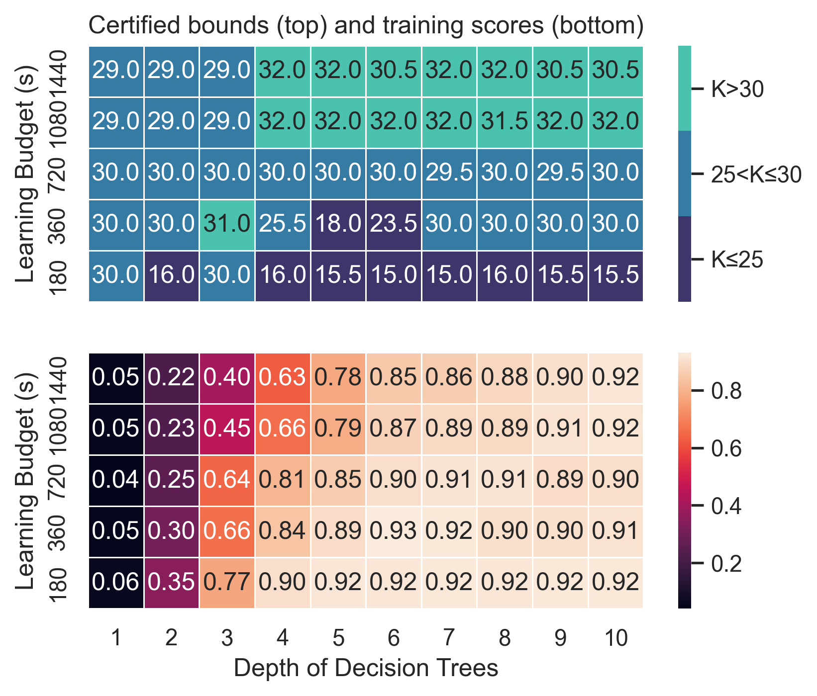
Figure 4: Varying the learning budget and tree depth on picor.pcregs-p0.

VIII Conclusion, limitations, and future work

We introduced Self-Driven Strategy Learning, a conceptually simple, easy-to-implement online learning approach for solving sets of related problems in automated reasoning. We presented the methodology formally as a set of transition rules and instantiated it in the context of Bounded Model Checking. Our experiments show that equipping a BMC-procedure with sdsl results in a significant performance boost, both in terms of certified bounds and solved instances, when comparing against state-of-the-art open-source model checkers.

One thing to consider when applying sdsl is that a good return on investment in learning depends on a sensible a priori choice of the strategy space. Another limitation is that when the problem set is small, gathering sufficient training data can be challenging. An intriguing question is whether a problem can be decomposed into sub-problems automatically in order to obtain sufficient data. Other future directions include alternative orders of applying the sdsl rules, applying sdsl to other automated reasoning tasks (e.g., symbolic execution, max-satisfiability, iterative abstraction refinement), and combining sdsl with offline learning and incremental solving.

Acknowledgments

We thank the anonymous reviewers for their careful reviews and constructive feedback. This work was supported in part by the National Science Foundation (grant 1269248) and by the Stanford Center for Automated Reasoning. Additionally, the NASA University Leadership initiative (grant #80NSSC20M0163) provided funds to assist the authors with their research, but this article solely reflects the opinions and conclusions of its authors and not any NASA entity.

Appendix A Versions of the solvers used in the BMC implementation and the experimental evaluation

Solver	Version
kissat	https://github.com/arminbiere/kissat/blob/97917ddf2
pono for generating SMTLIB files	https://github.com/anwu1219/pono/blob/ed11ef3eb
boolector	https://github.com/Boolector/boolector/blob/95859db82
pono for comparison	https://github.com/upscale-project/pono/blob/8b2a94649
avr	https://github.com/aman-goel/avr/blob/4cbceda5b
CaDiCaL	%****␣90appendix.tex␣Line␣25␣****https://github.com/arminbiere/cadical/tree/a5f15211d

Appendix B Other sdsl configurations

We also consider two additional sdsl configurations. $\textsc{kissat + {sdsl}}_{\textit{all}}$ is the same as $\textsc{kissat + {sdsl}}_{\textit{exp}}$ and $\textsc{kissat + {sdsl}}_{\textit{dev}}$, except it considers a strategy space of all 30 boolean flags of kissat. $\textsc{kissat + {sdsl}}^{\textit{tune}}_{\textit{exp}}$ operates on the larger strategy space $\mathcal{V}_{exp}$ and performs online tuning on the first $p$ BMC problems. Using a fixed $p$ for all benchmarks does not do this approach justice. Rather, $p$ is decided dynamically: $\textsc{kissat + {sdsl}}^{\textit{tune}}_{\textit{exp}}$ keeps solving the BMC problems and keep track of the total solving time $T$; when $m\cdot T$ exceeds the sampling budget $n$ for solving the current problem index $i$, it tunes on all the problems seen before $i$ using the conditional sampling procedure described in Sec. V. We have also tried other local search methods instead of the M-H algorithm, but the effect is similar.

The performance of these two configurations on the unsolved benchmarks is shown in Tab. VI. The step size is 1. $\textsc{kissat + {sdsl}}_{\textit{all}}$ performs significantly worse than kissat. This is not a surprise considering we are only allowed to draw 100 samples from $2^{30}$ possible candidates each time, which is not sufficient to capture the dependencies between parameter values or even land on any effective solving strategies. This suggests that the strategy space cannot be too large in the online learning setting. On the other hand, $\textsc{kissat + {sdsl}}^{\textit{tune}}_{\textit{exp}}$ does result in speedup in $t_{\textit{c.s.}}$ and improve upon kissat on 16 of the 24 instances. However, the performance gain is less significant compared to $\textsc{kissat + {sdsl}}_{\textit{dev}}$ (Tab. III). Moreover, the average certified bound by $\textsc{kissat + {sdsl}}^{\textit{tune}}_{\textit{exp}}$ is smaller than kissat, because the tuning appears to land on particularly harmful parameter settings on certain benchmarks (e.g., picor.pcregs-p0). This suggests that using empirical performance model (e.g., a Random Forest) is more robust than direct tuning in the online meta-algorithmic design setting.

TABLE VI: Evaluation of two other sdsl configurations $\textsc{kissat + {sdsl}}_{\textit{all}}$ and $\textsc{kissat + {sdsl}}^{\textit{tune}}_{\textit{exp}}$. The setup is the same as Tab. III

. step size = 1 step size = 1 $\textsc{kissat + {sdsl}}_{\textit{all}}$ kissat $\textsc{kissat + {sdsl}}^{\textit{tune}}_{\textit{exp}}$ kissat Benchmark ep $t_{\textit{learn}}$ $t_{\textit{c.s.}}$ $k$ $t_{\textit{c.s.}}$ $k$ ep $t_{\textit{learn}}$ $t_{\textit{c.s.}}$ $k$ $t_{\textit{c.s.}}$ $k$ arb.n2.w128.d64 9 1146 7044 34 684 54 1 924 6840 54 7198 54 arb.n2.w64.d64 7 769 6833 46 2908 53 1 740 6342 54 6515 53 arb.n2.w8.d128 8 1326 6485 51 5931 52 1 1074 5838 54 6795 52 arb.n3.w16.d128 8 1085 6959 51 5764 53 1 710 6779 53 7118 53 arb.n3.w64.d128 8 1057 6929 43 2260 53 1 727 6018 54 7132 53 arb.n3.w64.d64 9 978 6963 36 887 53 1 799 6033 54 7055 53 arb.n3.w8.d128 7 928 7154 35 879 53 1 710 6673 53 6996 53 arb.n4.w128.d64 8 1051 6630 50 4520 53 1 853 6563 53 6107 53 arb.n4.w16.d64 8 891 6584 34 747 53 1 799 6565 54 6599 53 arb.n4.w8.d64 7 1032 6715 51 5953 52 1 1282 6116 54 6659 52 arb.n5.w128.d64 8 974 7111 50 4729 53 1 695 6694 53 6731 53 circ.w128.d128 7 1028 6156 23 343 44 1 858 7192 44 6549 44 circ.w128.d64 7 935 6498 31 929 46 1 784 6448 46 6452 46 circ.w16.d128 7 1068 6920 39 1435 54 1 1091 6794 54 7179 54 circ.w64.d128 9 1034 7090 41 3161 48 1 638 4938 51 6895 48 dspf.p22 3 890 5614 24 1186 28 1 607 2496 35 5654 28 pgm.3.prop5 10 910 7151 125 4980 133 1 878 6976 127 5330 133 picor.AX.nom.p2 2 910 1164 13 158 15 1 150 3876 15 3636 15 picor.pcregs-p0 5 1079 6986 27 2427 30 1 730 20 16 20 30 picor.pcregs-p2 4 673 5347 27 1942 31 1 642 5481 24 596 31 shift.w128.d64 7 1070 7187 21 884 25 1 930 3380 28 5393 25 shift.w16.d128 7 1129 6672 26 347 39 1 912 4627 41 5817 39 shift.w32.d128 7 1011 7194 35 6273 35 1 1128 5988 35 6273 35 zipversa.p03 3 961 5814 61 6683 59 1 252 6424 57 6039 59 Mean 6.9 997 6466 40.6 2750 48.7 1 788 5629 48.5 5864 48.7

Appendix C Cross-examination of learned solving strategies

We study the effect of applying the learned parameter setting on one set of problems to other sets. In particular, we identify five parameter settings learned by $\textsc{kissat + {sdsl}}_{\textit{exp}}$ that have pairwise hamming distances of at least 6. For each of the five corresponding benchmarks, we identify the largest certified bound, and solved the corresponding SAT formula with kissat using each of the five parameter settings. A CPU timeout of 1800 seconds is given.

The benchmarks being considered and the learned parameter settings (only non-default values shown) are:

1. arb.n3.w64.d128: ands=0, chrono=0, eliminateint=50, forwardeffort=200, ifthenelse=0, probeint=10, stable=0, substituteeffort=20, vivifyeffort=200

2. circ.w128.d128: ands=0, bumpreasonsrate=1, chrono=0, eliminateint=50, eliminateocclim=20, stable=0, vivifyeffort=200

3. pgm.3.prop5: ands=0, forwardeffort=200, stable=0, subsumeocclim=10, vivifyeffort=200

4. picor.pcregs-p2: eliminateocclim=20, forwardeffort=200, ifthenelse=0

5. shift.w32.d128: bumpreasonsrate=1, eliminateint=50, eliminateocclim=20, forwardeffort=200, probeint=10, stable=0, substituteeffort=20, subsumeocclim=10, vivifyeffort=200

The result is shown below:

	Problem 1	Problem 2	Problem 3	Problem 4	Problem 5
Strategy 1	445	978	210	–	–
Strategy 2	405	637	241	–	1357
Strategy 3	507	761	188	–	–
Strategy 4	1107	864	256	1434	–
Strategy 5	434	817	215	–	968

The strategy learned specifically for a benchmark generally performs better than the alternative strategies. In particular, Problem 4 can be solved within the time limit only using Strategy 4. On the other hand, solving Problem 5 using Strategy 4 results in a timeout. This suggests that the optimal strategies for different instances might contradict with one another.

Appendix D Effect of Incremental Solving

We hoped to also study the interplay between sdsl and incremental solving. However, the effect of incremental solving is mixed on the 24 unsolved bit-vector benchmarks from HWMCC. We focus on the state-of-the-art incremental SAT solver CaDiCaL, which is used by pono under-the-hood to solve the set of problems from a BMC run. We compare pono with the BMC procedure we implement using the non-incremental mode of CaDiCaL. The bounds certified by running BMC with step size 1 for 2 hours are shown in Tab. VII. While pono, which runs the incremental mode of CaDiCaL, certifies a larger bound on barely more than half of the benchmarks, the non-incremental mode of CaDiCaL can certify larger bounds overall. This experiment suggests that it is worth revisiting BMC-specific incremental solving techniques [16] before investigating the interplay between sdsl and incremental solving, which we do believe is an important topic.

TABLE VII: The certified bounds by pono and a CaDiCaL-based BMC procedure.

Benchmark	pono	CaDiCaL
arb.n2.w128.d64	45	44
arb.n2.w64.d64	48	45
arb.n2.w8.d128	45	45
arb.n3.w16.d128	48	44
arb.n3.w64.d128	44	45
arb.n3.w64.d64	46	44
arb.n3.w8.d128	46	45
arb.n4.w128.d64	46	44
arb.n4.w16.d64	49	44
arb.n4.w8.d64	48	45
arb.n5.w128.d64	47	44
circ.w128.d128	39	44
circ.w128.d64	39	43
circ.w16.d128	47	47
circ.w64.d128	44	45
dspf.p22	27	34
pgm.3.prop5	131	131
picor.AX.nom.p2	14	15
picor.pcregs-p0	30	27
picor.pcregs-p2	31	27
shift.w128.d64	21	22
shift.w16.d128	28	39
shift.w32.d128	27	33
zipversa.p03	45	43
Mean	43.1	43.3

Appendix E Executions of all BMC configurations with step size 1 on the unsolved bitvector HWMCC benchmarks

Appendix F Duration of each training epoch

The duration (in seconds) of each training epoch during the run of $\textsc{kissat + {sdsl}}_{\textit{exp}}$ on the unsolved bitvector HWMCC benchmarks with step size 1 is reported in the table below:

Benchmark	$ep_{1}$, $ep_{2}$, …
arb.n2.w128.d64	6, 12, 21, 34, 56, 87, 120, 171, 205, 296
arb.n2.w64.d64	12, 17, 30, 44, 76, 132, 147, 192, 255
arb.n2.w8.d128	4, 12, 17, 29, 46, 84, 112, 175, 219, 300
arb.n3.w16.d128	10, 18, 35, 63, 86, 133, 162, 253, 143
arb.n3.w64.d128	6, 12, 25, 39, 76, 119, 145, 233, 146, 223
arb.n3.w64.d64	6, 11, 22, 38, 56, 93, 130, 185, 246, 162
arb.n3.w8.d128	10, 17, 36, 51, 81, 129, 216, 241, 171
arb.n4.w128.d64	10, 14, 33, 50, 71, 144, 166, 184, 259
arb.n4.w16.d64	6, 10, 19, 36, 56, 88, 136, 198, 251, 150
arb.n4.w8.d64	6, 10, 19, 35, 53, 82, 107, 180, 239, 315
arb.n5.w128.d64	12, 20, 34, 50, 81, 140, 187, 247, 304
circ.w128.d128	5, 15, 35, 48, 122, 220, 373
circ.w128.d64	5, 15, 25, 65, 129, 169, 286, 161
circ.w16.d128	2, 6, 13, 25, 47, 80, 110, 137, 217, 200, 94
circ.w64.d128	3, 6, 11, 22, 50, 82, 142, 219, 300
dspf.p22	178, 286, 274, 317
pgm.3.prop5	55, 73, 85, 106, 109, 85, 83, 111, 200, 78
picor.AX.nom.p2	102, 770
picor.pcregs-p0	21, 68, 242, 360, 275
picor.pcregs-p2	21, 103, 180, 312, 200, 48
shift.w128.d64	5, 12, 29, 94, 160, 203, 327
shift.w16.d128	2, 7, 24, 55, 80, 118, 176, 349, 239
shift.w32.d128	3, 7, 32, 74, 89, 152, 236, 197
zipversa.p03	40, 146, 208, 302, 398

Appendix G Raw Results on the satisfiable and unknown bit-vector benchmarks from HWMCC’20

Note: for pono portfolio and AVR portfolio, the status is MEMOUT if and only if none of the threads in the portfolio solve the problem and at least one of the threads runs out of the 8GB memory limit.

Benchmark	Configuration	Status	Time	Memory
anderson.3.prop1-back-serstep.btor2	$\textsc{kissat + {sdsl}}_{\textit{exp}}$	SAT	2.3	74.3
arbitrated_top_n2_w128_d32_e0.btor2	$\textsc{kissat + {sdsl}}_{\textit{exp}}$	SAT	227.3	353.3
arbitrated_top_n2_w128_d64_e0.btor2	$\textsc{kissat + {sdsl}}_{\textit{exp}}$	SAT	3336.7	1110.0
arbitrated_top_n2_w64_d64_e0.btor2	$\textsc{kissat + {sdsl}}_{\textit{exp}}$	SAT	2566.7	659.1
arbitrated_top_n2_w8_d128_e0.btor2	$\textsc{kissat + {sdsl}}_{\textit{exp}}$	TIMEOUT	3600.0	402.9
arbitrated_top_n2_w8_d16_e0.btor2	$\textsc{kissat + {sdsl}}_{\textit{exp}}$	SAT	27.3	73.4
arbitrated_top_n2_w8_d32_e0.btor2	$\textsc{kissat + {sdsl}}_{\textit{exp}}$	SAT	131.3	108.6
arbitrated_top_n3_w16_d128_e0.btor2	$\textsc{kissat + {sdsl}}_{\textit{exp}}$	TIMEOUT	3600.0	659.4
arbitrated_top_n3_w16_d32_e0.btor2	$\textsc{kissat + {sdsl}}_{\textit{exp}}$	SAT	150.5	150.8
arbitrated_top_n3_w32_d16_e0.btor2	$\textsc{kissat + {sdsl}}_{\textit{exp}}$	SAT	38.0	96.9
arbitrated_top_n3_w64_d128_e0.btor2	$\textsc{kissat + {sdsl}}_{\textit{exp}}$	TIMEOUT	3601.0	1524.1
arbitrated_top_n3_w64_d64_e0.btor2	$\textsc{kissat + {sdsl}}_{\textit{exp}}$	SAT	3127.1	883.4
arbitrated_top_n3_w8_d128_e0.btor2	$\textsc{kissat + {sdsl}}_{\textit{exp}}$	TIMEOUT	3600.0	709.7
arbitrated_top_n3_w8_d16_e0.btor2	$\textsc{kissat + {sdsl}}_{\textit{exp}}$	SAT	33.1	81.4
arbitrated_top_n4_w128_d16_e0.btor2	$\textsc{kissat + {sdsl}}_{\textit{exp}}$	SAT	77.6	204.6
arbitrated_top_n4_w128_d64_e0.btor2	$\textsc{kissat + {sdsl}}_{\textit{exp}}$	SAT	3053.0	2309.1
arbitrated_top_n4_w16_d16_e0.btor2	$\textsc{kissat + {sdsl}}_{\textit{exp}}$	SAT	37.5	95.3
arbitrated_top_n4_w16_d32_e0.btor2	$\textsc{kissat + {sdsl}}_{\textit{exp}}$	SAT	157.2	192.6
arbitrated_top_n4_w16_d64_e0.btor2	$\textsc{kissat + {sdsl}}_{\textit{exp}}$	SAT	2441.6	529.6
arbitrated_top_n4_w32_d32_e0.btor2	$\textsc{kissat + {sdsl}}_{\textit{exp}}$	SAT	243.2	240.6
arbitrated_top_n4_w64_d32_e0.btor2	$\textsc{kissat + {sdsl}}_{\textit{exp}}$	SAT	236.5	369.2
arbitrated_top_n4_w8_d64_e0.btor2	$\textsc{kissat + {sdsl}}_{\textit{exp}}$	SAT	2376.1	418.3
arbitrated_top_n5_w128_d64_e0.btor2	$\textsc{kissat + {sdsl}}_{\textit{exp}}$	SAT	3555.6	2743.1
arbitrated_top_n5_w128_d8_e0.btor2	$\textsc{kissat + {sdsl}}_{\textit{exp}}$	SAT	63.0	187.3
arbitrated_top_n5_w32_d32_e0.btor2	$\textsc{kissat + {sdsl}}_{\textit{exp}}$	SAT	194.4	309.6
arbitrated_top_n5_w64_d16_e0.btor2	$\textsc{kissat + {sdsl}}_{\textit{exp}}$	SAT	56.7	151.3
arbitrated_top_n5_w8_d32_e0.btor2	$\textsc{kissat + {sdsl}}_{\textit{exp}}$	SAT	158.0	171.1
at.6.prop1-back-serstep.btor2	$\textsc{kissat + {sdsl}}_{\textit{exp}}$	SAT	6.4	78.9
blocks.4.prop1-back-serstep.btor2	$\textsc{kissat + {sdsl}}_{\textit{exp}}$	SAT	121.4	128.8
brp2.2.prop1-func-interl.btor2	$\textsc{kissat + {sdsl}}_{\textit{exp}}$	SAT	206.7	191.3
brp2.3.prop1-back-serstep.btor2	$\textsc{kissat + {sdsl}}_{\textit{exp}}$	SAT	96.3	166.8
buggy_ridecore.btor	$\textsc{kissat + {sdsl}}_{\textit{exp}}$	SAT	57.9	912.0
circular_pointer_top_w128_d128_e0.btor2	$\textsc{kissat + {sdsl}}_{\textit{exp}}$	TIMEOUT	3600.1	4437.9
circular_pointer_top_w128_d64_e0.btor2	$\textsc{kissat + {sdsl}}_{\textit{exp}}$	TIMEOUT	3600.1	2446.4
circular_pointer_top_w128_d8_e0.btor2	$\textsc{kissat + {sdsl}}_{\textit{exp}}$	SAT	4.5	102.1
circular_pointer_top_w16_d128_e0.btor2	$\textsc{kissat + {sdsl}}_{\textit{exp}}$	TIMEOUT	3600.0	661.7
circular_pointer_top_w16_d32_e0.btor2	$\textsc{kissat + {sdsl}}_{\textit{exp}}$	SAT	737.7	114.8
circular_pointer_top_w32_d16_e0.btor2	$\textsc{kissat + {sdsl}}_{\textit{exp}}$	SAT	94.0	91.6
circular_pointer_top_w32_d32_e0.btor2	$\textsc{kissat + {sdsl}}_{\textit{exp}}$	SAT	455.8	269.0
circular_pointer_top_w64_d128_e0.btor2	$\textsc{kissat + {sdsl}}_{\textit{exp}}$	TIMEOUT	3600.1	2074.4
circular_pointer_top_w64_d8_e0.btor2	$\textsc{kissat + {sdsl}}_{\textit{exp}}$	SAT	60.0	82.6
circular_pointer_top_w8_d16_e0.btor2	$\textsc{kissat + {sdsl}}_{\textit{exp}}$	SAT	34.0	70.2
dspfilters_fastfir_second-p22.btor	$\textsc{kissat + {sdsl}}_{\textit{exp}}$	TIMEOUT	3600.0	434.1
krebs.3.prop1-func-interl.btor2	$\textsc{kissat + {sdsl}}_{\textit{exp}}$	SAT	102.1	151.5
mul7.btor2	$\textsc{kissat + {sdsl}}_{\textit{exp}}$	SAT	6.6	796.9
mul9.btor2	$\textsc{kissat + {sdsl}}_{\textit{exp}}$	TIMEOUT	3600.0	184.2
peg_solitaire.3.prop1-back-serstep.btor2	$\textsc{kissat + {sdsl}}_{\textit{exp}}$	SAT	61.2	157.3
pgm_protocol.3.prop5-func-interl.btor2	$\textsc{kissat + {sdsl}}_{\textit{exp}}$	TIMEOUT	3600.9	2768.9
picorv32-pcregs-p0.btor	$\textsc{kissat + {sdsl}}_{\textit{exp}}$	TIMEOUT	3600.0	279.0
picorv32-pcregs-p2.btor	$\textsc{kissat + {sdsl}}_{\textit{exp}}$	TIMEOUT	3600.0	273.2
picorv32_mutAX_nomem-p0.btor	$\textsc{kissat + {sdsl}}_{\textit{exp}}$	SAT	168.4	453.0
picorv32_mutAX_nomem-p2.btor	$\textsc{kissat + {sdsl}}_{\textit{exp}}$	SAT	224.9	453.4
picorv32_mutAX_nomem-p5.btor	$\textsc{kissat + {sdsl}}_{\textit{exp}}$	SAT	149.1	451.5
picorv32_mutAY_nomem-p1.btor	$\textsc{kissat + {sdsl}}_{\textit{exp}}$	SAT	28.6	363.8
picorv32_mutAY_nomem-p4.btor	$\textsc{kissat + {sdsl}}_{\textit{exp}}$	SAT	36.4	366.9
picorv32_mutAY_nomem-p6.btor	$\textsc{kissat + {sdsl}}_{\textit{exp}}$	SAT	95.6	346.2
picorv32_mutBX_nomem-p0.btor	$\textsc{kissat + {sdsl}}_{\textit{exp}}$	SAT	118.0	455.0
picorv32_mutBX_nomem-p5.btor	$\textsc{kissat + {sdsl}}_{\textit{exp}}$	SAT	112.3	450.0
picorv32_mutBX_nomem-p8.btor	$\textsc{kissat + {sdsl}}_{\textit{exp}}$	SAT	89.8	453.3
picorv32_mutBY_nomem-p1.btor	$\textsc{kissat + {sdsl}}_{\textit{exp}}$	SAT	81.7	367.2
picorv32_mutBY_nomem-p3.btor	$\textsc{kissat + {sdsl}}_{\textit{exp}}$	SAT	104.5	368.2
picorv32_mutBY_nomem-p4.btor	$\textsc{kissat + {sdsl}}_{\textit{exp}}$	SAT	44.5	356.6
picorv32_mutBY_nomem-p6.btor	$\textsc{kissat + {sdsl}}_{\textit{exp}}$	SAT	118.2	346.8

Benchmark	Configuration	Status	Time	Memory
picorv32_mutBY_nomem-p7.btor	$\textsc{kissat + {sdsl}}_{\textit{exp}}$	SAT	50.7	350.5
picorv32_mutCX_nomem-p0.btor	$\textsc{kissat + {sdsl}}_{\textit{exp}}$	SAT	114.4	458.1
picorv32_mutCX_nomem-p8.btor	$\textsc{kissat + {sdsl}}_{\textit{exp}}$	SAT	253.5	454.7
picorv32_mutCY_nomem-p0.btor	$\textsc{kissat + {sdsl}}_{\textit{exp}}$	SAT	102.9	360.7
picorv32_mutCY_nomem-p3.btor	$\textsc{kissat + {sdsl}}_{\textit{exp}}$	SAT	98.2	364.0
rast-p03.btor	$\textsc{kissat + {sdsl}}_{\textit{exp}}$	SAT	1.5	68.9
rast-p06.btor	$\textsc{kissat + {sdsl}}_{\textit{exp}}$	SAT	1.6	69.1
rast-p18.btor	$\textsc{kissat + {sdsl}}_{\textit{exp}}$	SAT	1.7	68.8
rast-p19.btor	$\textsc{kissat + {sdsl}}_{\textit{exp}}$	SAT	1.7	69.0
ridecore.btor	$\textsc{kissat + {sdsl}}_{\textit{exp}}$	SAT	45.2	909.8
shift_register_top_w128_d16_e0.btor2	$\textsc{kissat + {sdsl}}_{\textit{exp}}$	TIMEOUT	3600.0	192.3
shift_register_top_w128_d64_e0.btor2	$\textsc{kissat + {sdsl}}_{\textit{exp}}$	TIMEOUT	3600.0	325.2
shift_register_top_w16_d128_e0.btor2	$\textsc{kissat + {sdsl}}_{\textit{exp}}$	TIMEOUT	3600.0	186.8
shift_register_top_w16_d16_e0.btor2	$\textsc{kissat + {sdsl}}_{\textit{exp}}$	SAT	239.3	103.7
shift_register_top_w16_d32_e0.btor2	$\textsc{kissat + {sdsl}}_{\textit{exp}}$	TIMEOUT	3600.0	150.8
shift_register_top_w16_d64_e0.btor2	$\textsc{kissat + {sdsl}}_{\textit{exp}}$	TIMEOUT	3600.0	167.6
shift_register_top_w16_d8_e0.btor2	$\textsc{kissat + {sdsl}}_{\textit{exp}}$	SAT	50.1	67.4
shift_register_top_w32_d128_e0.btor2	$\textsc{kissat + {sdsl}}_{\textit{exp}}$	TIMEOUT	3600.0	232.2
shift_register_top_w32_d16_e0.btor2	$\textsc{kissat + {sdsl}}_{\textit{exp}}$	SAT	561.5	114.2
shift_register_top_w32_d8_e0.btor2	$\textsc{kissat + {sdsl}}_{\textit{exp}}$	SAT	64.3	73.5
shift_register_top_w64_d8_e0.btor2	$\textsc{kissat + {sdsl}}_{\textit{exp}}$	SAT	5.7	79.3
shift_register_top_w8_d128_e0.btor2	$\textsc{kissat + {sdsl}}_{\textit{exp}}$	TIMEOUT	3600.0	160.9
stack-p1.btor	$\textsc{kissat + {sdsl}}_{\textit{exp}}$	SAT	3.1	127.4
vis_arrays_am2901.btor2	$\textsc{kissat + {sdsl}}_{\textit{exp}}$	SAT	47.8	75.9
vis_arrays_buf_bug.btor2	$\textsc{kissat + {sdsl}}_{\textit{exp}}$	SAT	11.4	70.1
zipversa_composecrc_prf-p03.btor	$\textsc{kissat + {sdsl}}_{\textit{exp}}$	TIMEOUT	3600.0	207.5
anderson.3.prop1-back-serstep.btor2	kissat	SAT	1.3	73.6
anderson.3.prop1-back-serstep.btor2	kissat	SAT	2.4	73.7
arbitrated_top_n2_w128_d32_e0.btor2	kissat	SAT	175.7	351.4
arbitrated_top_n2_w128_d64_e0.btor2	kissat	TIMEOUT	3600.0	885.9
arbitrated_top_n2_w64_d64_e0.btor2	kissat	TIMEOUT	3600.0	571.5
arbitrated_top_n2_w8_d128_e0.btor2	kissat	TIMEOUT	3600.0	407.4
arbitrated_top_n2_w8_d16_e0.btor2	kissat	SAT	5.5	71.5
arbitrated_top_n2_w8_d32_e0.btor2	kissat	SAT	124.4	106.5
arbitrated_top_n3_w16_d128_e0.btor2	kissat	TIMEOUT	3600.0	611.4
arbitrated_top_n3_w16_d32_e0.btor2	kissat	SAT	106.7	148.9
arbitrated_top_n3_w32_d16_e0.btor2	kissat	SAT	8.5	94.9
arbitrated_top_n3_w64_d128_e0.btor2	kissat	TIMEOUT	3601.0	1378.8
arbitrated_top_n3_w64_d64_e0.btor2	kissat	TIMEOUT	3600.0	754.8
arbitrated_top_n3_w8_d128_e0.btor2	kissat	TIMEOUT	3600.0	520.7
arbitrated_top_n3_w8_d16_e0.btor2	kissat	SAT	8.2	77.4
arbitrated_top_n4_w128_d16_e0.btor2	kissat	SAT	12.6	203.6
arbitrated_top_n4_w128_d64_e0.btor2	kissat	TIMEOUT	3601.0	1718.6
arbitrated_top_n4_w16_d16_e0.btor2	kissat	SAT	6.5	92.6
arbitrated_top_n4_w16_d32_e0.btor2	kissat	SAT	126.4	192.4
arbitrated_top_n4_w16_d64_e0.btor2	kissat	TIMEOUT	3600.0	427.3
arbitrated_top_n4_w32_d32_e0.btor2	kissat	SAT	122.7	236.7
arbitrated_top_n4_w64_d32_e0.btor2	kissat	SAT	136.0	368.6
arbitrated_top_n4_w8_d64_e0.btor2	kissat	TIMEOUT	3600.0	341.1
arbitrated_top_n5_w128_d64_e0.btor2	kissat	TIMEOUT	3601.0	2329.3
arbitrated_top_n5_w128_d8_e0.btor2	kissat	SAT	6.3	187.2
arbitrated_top_n5_w32_d32_e0.btor2	kissat	SAT	149.8	309.3
arbitrated_top_n5_w64_d16_e0.btor2	kissat	SAT	9.2	150.7
arbitrated_top_n5_w8_d32_e0.btor2	kissat	SAT	115.1	171.0
at.6.prop1-back-serstep.btor2	kissat	SAT	6.2	76.7
blocks.4.prop1-back-serstep.btor2	kissat	SAT	78.1	127.2
brp2.2.prop1-func-interl.btor2	kissat	SAT	123.5	191.4
brp2.3.prop1-back-serstep.btor2	kissat	SAT	13.3	165.8
buggy_ridecore.btor	kissat	SAT	59.2	912.6
circular_pointer_top_w128_d128_e0.btor2	kissat	TIMEOUT	3600.1	4260.6
circular_pointer_top_w128_d64_e0.btor2	kissat	TIMEOUT	3600.1	2539.0
circular_pointer_top_w128_d8_e0.btor2	kissat	SAT	4.8	102.2
circular_pointer_top_w16_d128_e0.btor2	kissat	TIMEOUT	3600.0	649.2
circular_pointer_top_w16_d32_e0.btor2	kissat	SAT	161.1	188.8
circular_pointer_top_w32_d16_e0.btor2	kissat	SAT	19.9	88.8
circular_pointer_top_w32_d32_e0.btor2	kissat	SAT	338.8	267.5
circular_pointer_top_w64_d128_e0.btor2	kissat	TIMEOUT	3600.1	2072.8
circular_pointer_top_w64_d8_e0.btor2	kissat	SAT	3.3	81.2
circular_pointer_top_w8_d16_e0.btor2	kissat	SAT	5.9	67.1
dspfilters_fastfir_second-p22.btor	kissat	TIMEOUT	3600.0	434.9
krebs.3.prop1-func-interl.btor2	kissat	SAT	19.2	148.4
mul7.btor2	kissat	SAT	7.2	796.4

Benchmark	Configuration	Status	Time	Memory
mul9.btor2	kissat	TIMEOUT	3600.0	177.4
peg_solitaire.3.prop1-back-serstep.btor2	kissat	SAT	59.6	157.2
pgm_protocol.3.prop5-func-interl.btor2	kissat	TIMEOUT	3600.9	2771.0
picorv32-pcregs-p0.btor	kissat	TIMEOUT	3600.0	280.1
picorv32-pcregs-p2.btor	kissat	TIMEOUT	3600.0	274.2
picorv32_mutAX_nomem-p0.btor	kissat	SAT	154.0	452.6
picorv32_mutAX_nomem-p2.btor	kissat	SAT	140.0	452.6
picorv32_mutAX_nomem-p5.btor	kissat	SAT	82.7	449.8
picorv32_mutAY_nomem-p1.btor	kissat	SAT	26.4	361.7
picorv32_mutAY_nomem-p4.btor	kissat	SAT	33.1	366.5
picorv32_mutAY_nomem-p6.btor	kissat	SAT	41.6	345.0
picorv32_mutBX_nomem-p0.btor	kissat	SAT	113.2	453.5
picorv32_mutBX_nomem-p5.btor	kissat	SAT	64.4	448.8
picorv32_mutBX_nomem-p8.btor	kissat	SAT	89.2	453.8
picorv32_mutBY_nomem-p1.btor	kissat	SAT	87.2	367.9
picorv32_mutBY_nomem-p3.btor	kissat	SAT	103.4	368.4
picorv32_mutBY_nomem-p4.btor	kissat	SAT	41.4	357.8
picorv32_mutBY_nomem-p6.btor	kissat	SAT	21.6	344.5
picorv32_mutBY_nomem-p7.btor	kissat	SAT	57.2	348.9
picorv32_mutCX_nomem-p0.btor	kissat	SAT	57.3	456.5
picorv32_mutCX_nomem-p8.btor	kissat	SAT	216.2	453.9
picorv32_mutCY_nomem-p0.btor	kissat	SAT	99.7	360.5
picorv32_mutCY_nomem-p3.btor	kissat	SAT	61.8	363.2
rast-p03.btor	kissat	SAT	1.9	69.6
rast-p06.btor	kissat	SAT	1.9	69.3
rast-p18.btor	kissat	SAT	2.1	69.7
rast-p19.btor	kissat	SAT	2.1	68.9
ridecore.btor	kissat	SAT	49.5	912.2
shift_register_top_w128_d16_e0.btor2	kissat	TIMEOUT	3600.0	191.3
shift_register_top_w128_d64_e0.btor2	kissat	TIMEOUT	3600.0	323.3
shift_register_top_w16_d128_e0.btor2	kissat	TIMEOUT	3600.0	176.6
shift_register_top_w16_d16_e0.btor2	kissat	SAT	323.0	89.3
shift_register_top_w16_d32_e0.btor2	kissat	TIMEOUT	3600.0	154.2
shift_register_top_w16_d64_e0.btor2	kissat	TIMEOUT	3600.0	168.9
shift_register_top_w16_d8_e0.btor2	kissat	SAT	3.3	66.5
shift_register_top_w32_d128_e0.btor2	kissat	TIMEOUT	3600.0	228.6
shift_register_top_w32_d16_e0.btor2	kissat	SAT	2448.0	112.1
shift_register_top_w32_d8_e0.btor2	kissat	SAT	4.8	70.3
shift_register_top_w64_d8_e0.btor2	kissat	SAT	6.5	79.4
shift_register_top_w8_d128_e0.btor2	kissat	TIMEOUT	3600.0	157.8
stack-p1.btor	kissat	SAT	3.5	127.0
vis_arrays_am2901.btor2	kissat	SAT	2.5	73.6
vis_arrays_buf_bug.btor2	kissat	SAT	2.5	64.5
zipversa_composecrc_prf-p03.btor	kissat	TIMEOUT	3600.0	205.1
anderson.3.prop1-back-serstep.btor2	pono portfolio	SAT	0.1	9.0
arbitrated_top_n2_w128_d32_e0.btor2	pono portfolio	SAT	605.6	171.0
arbitrated_top_n2_w128_d64_e0.btor2	pono portfolio	MEMOUT	1785.3	8000.0
arbitrated_top_n2_w64_d64_e0.btor2	pono portfolio	MEMOUT	1255.8	8000.0
arbitrated_top_n2_w8_d128_e0.btor2	pono portfolio	MEMOUT	2957.6	8000.0
arbitrated_top_n2_w8_d16_e0.btor2	pono portfolio	SAT	0.7	13.1
arbitrated_top_n2_w8_d32_e0.btor2	pono portfolio	SAT	510.4	116.2
arbitrated_top_n3_w16_d128_e0.btor2	pono portfolio	MEMOUT	2283.7	8000.0
arbitrated_top_n3_w16_d32_e0.btor2	pono portfolio	SAT	516.9	127.6
arbitrated_top_n3_w32_d16_e0.btor2	pono portfolio	SAT	1.7	21.1
arbitrated_top_n3_w64_d128_e0.btor2	pono portfolio	MEMOUT	851.7	8000.0
arbitrated_top_n3_w64_d64_e0.btor2	pono portfolio	MEMOUT	1397.0	8000.0
arbitrated_top_n3_w8_d128_e0.btor2	pono portfolio	TIMEOUT	3600.0	351.5
arbitrated_top_n3_w8_d16_e0.btor2	pono portfolio	SAT	0.8	17.0
arbitrated_top_n4_w128_d16_e0.btor2	pono portfolio	SAT	2.8	46.8
arbitrated_top_n4_w128_d64_e0.btor2	pono portfolio	MEMOUT	1285.6	8000.0
arbitrated_top_n4_w16_d16_e0.btor2	pono portfolio	SAT	1.9	24.2
arbitrated_top_n4_w16_d32_e0.btor2	pono portfolio	SAT	602.8	137.4
arbitrated_top_n4_w16_d64_e0.btor2	pono portfolio	MEMOUT	1940.1	8000.0
arbitrated_top_n4_w32_d32_e0.btor2	pono portfolio	SAT	570.9	135.5
arbitrated_top_n4_w64_d32_e0.btor2	pono portfolio	SAT	225.7	122.3
arbitrated_top_n4_w8_d64_e0.btor2	pono portfolio	MEMOUT	2839.4	8000.0
arbitrated_top_n5_w128_d64_e0.btor2	pono portfolio	MEMOUT	869.9	8000.0
arbitrated_top_n5_w128_d8_e0.btor2	pono portfolio	SAT	0.5	23.0
arbitrated_top_n5_w32_d32_e0.btor2	pono portfolio	SAT	520.7	154.8
arbitrated_top_n5_w64_d16_e0.btor2	pono portfolio	SAT	2.7	40.9
arbitrated_top_n5_w8_d32_e0.btor2	pono portfolio	SAT	494.0	120.9
at.6.prop1-back-serstep.btor2	pono portfolio	SAT	1.6	27.1

Benchmark	Configuration	Status	Time	Memory
blocks.4.prop1-back-serstep.btor2	pono portfolio	SAT	333.3	301.0
brp2.2.prop1-func-interl.btor2	pono portfolio	SAT	1795.6	2202.0
brp2.3.prop1-back-serstep.btor2	pono portfolio	SAT	25.5	124.2
buggy_ridecore.btor	pono portfolio	SAT	137.7	846.6
circular_pointer_top_w128_d128_e0.btor2	pono portfolio	MEMOUT	252.4	8000.0
circular_pointer_top_w128_d64_e0.btor2	pono portfolio	MEMOUT	1956.7	8000.0
circular_pointer_top_w128_d8_e0.btor2	pono portfolio	SAT	1.1	34.2
circular_pointer_top_w16_d128_e0.btor2	pono portfolio	TIMEOUT	3600.0	3342.7
circular_pointer_top_w16_d32_e0.btor2	pono portfolio	SAT	492.1	106.0
circular_pointer_top_w32_d16_e0.btor2	pono portfolio	SAT	2.5	42.1
circular_pointer_top_w32_d32_e0.btor2	pono portfolio	SAT	220.3	153.6
circular_pointer_top_w64_d128_e0.btor2	pono portfolio	TIMEOUT	3600.0	1358.3
circular_pointer_top_w64_d8_e0.btor2	pono portfolio	SAT	0.7	23.2
circular_pointer_top_w8_d16_e0.btor2	pono portfolio	SAT	1.1	12.5
dspfilters_fastfir_second-p22.btor	pono portfolio	TIMEOUT	3600.0	7609.3
krebs.3.prop1-func-interl.btor2	pono portfolio	SAT	26.2	107.8
mul7.btor2	pono portfolio	SAT	1.7	171.4
mul9.btor2	pono portfolio	SAT	167.9	1575.7
peg_solitaire.3.prop1-back-serstep.btor2	pono portfolio	SAT	138.4	222.4
pgm_protocol.3.prop5-func-interl.btor2	pono portfolio	TIMEOUT	3600.0	212.9
picorv32-pcregs-p0.btor	pono portfolio	MEMOUT	3013.4	8000.0
picorv32-pcregs-p2.btor	pono portfolio	MEMOUT	3020.1	8000.0
picorv32_mutAX_nomem-p0.btor	pono portfolio	SAT	106.4	507.7
picorv32_mutAX_nomem-p2.btor	pono portfolio	SAT	61.4	493.5
picorv32_mutAX_nomem-p5.btor	pono portfolio	SAT	87.6	478.6
picorv32_mutAY_nomem-p1.btor	pono portfolio	SAT	65.6	482.7
picorv32_mutAY_nomem-p4.btor	pono portfolio	SAT	35.6	377.6
picorv32_mutAY_nomem-p6.btor	pono portfolio	SAT	22.9	387.8
picorv32_mutBX_nomem-p0.btor	pono portfolio	SAT	94.8	510.8
picorv32_mutBX_nomem-p5.btor	pono portfolio	SAT	145.5	504.0
picorv32_mutBX_nomem-p8.btor	pono portfolio	SAT	281.3	567.1
picorv32_mutBY_nomem-p1.btor	pono portfolio	SAT	35.6	431.3
picorv32_mutBY_nomem-p3.btor	pono portfolio	SAT	36.2	398.4
picorv32_mutBY_nomem-p4.btor	pono portfolio	SAT	49.2	383.0
picorv32_mutBY_nomem-p6.btor	pono portfolio	SAT	55.3	398.7
picorv32_mutBY_nomem-p7.btor	pono portfolio	SAT	225.8	407.6
picorv32_mutCX_nomem-p0.btor	pono portfolio	SAT	136.9	493.7
picorv32_mutCX_nomem-p8.btor	pono portfolio	SAT	276.9	581.9
picorv32_mutCY_nomem-p0.btor	pono portfolio	SAT	76.8	448.1
picorv32_mutCY_nomem-p3.btor	pono portfolio	SAT	27.4	398.5
rast-p03.btor	pono portfolio	SAT	0.2	47.1
rast-p06.btor	pono portfolio	SAT	0.1	23.7
rast-p18.btor	pono portfolio	SAT	0.1	23.6
rast-p19.btor	pono portfolio	SAT	0.1	23.6
ridecore.btor	pono portfolio	SAT	135.3	852.6
shift_register_top_w128_d16_e0.btor2	pono portfolio	SAT	413.0	411.6
shift_register_top_w128_d64_e0.btor2	pono portfolio	MEMOUT	1650.7	8000.0
shift_register_top_w16_d128_e0.btor2	pono portfolio	MEMOUT	2027.6	8000.0
shift_register_top_w16_d16_e0.btor2	pono portfolio	SAT	223.3	99.1
shift_register_top_w16_d32_e0.btor2	pono portfolio	MEMOUT	1450.3	8000.0
shift_register_top_w16_d64_e0.btor2	pono portfolio	MEMOUT	1736.5	8000.0
shift_register_top_w16_d8_e0.btor2	pono portfolio	SAT	0.3	9.5
shift_register_top_w32_d128_e0.btor2	pono portfolio	MEMOUT	1978.3	8000.0
shift_register_top_w32_d16_e0.btor2	pono portfolio	SAT	722.1	145.2
shift_register_top_w32_d8_e0.btor2	pono portfolio	SAT	0.4	13.8
shift_register_top_w64_d8_e0.btor2	pono portfolio	SAT	2.4	36.4
shift_register_top_w8_d128_e0.btor2	pono portfolio	MEMOUT	2028.7	8000.0
stack-p1.btor	pono portfolio	SAT	0.1	9.9
vis_arrays_am2901.btor2	pono portfolio	SAT	0.4	10.8
vis_arrays_buf_bug.btor2	pono portfolio	SAT	0.4	7.2
zipversa_composecrc_prf-p03.btor	pono portfolio	TIMEOUT	3600.0	2998.6
anderson.3.prop1-back-serstep.btor2	AVR portfolio	SAT	0.2	26.0
arbitrated_top_n2_w128_d32_e0.btor2	AVR portfolio	SAT	455.4	240.1
arbitrated_top_n2_w128_d64_e0.btor2	AVR portfolio	MEMOUT	1781.9	8000.0
arbitrated_top_n2_w64_d64_e0.btor2	AVR portfolio	MEMOUT	1437.3	8000.0
arbitrated_top_n2_w8_d128_e0.btor2	AVR portfolio	MEMOUT	1304.1	8000.0
arbitrated_top_n2_w8_d16_e0.btor2	AVR portfolio	SAT	6.1	47.6
arbitrated_top_n2_w8_d32_e0.btor2	AVR portfolio	SAT	452.9	160.4
arbitrated_top_n3_w16_d128_e0.btor2	AVR portfolio	MEMOUT	1509.6	8000.0
arbitrated_top_n3_w16_d32_e0.btor2	AVR portfolio	SAT	549.1	210.1
arbitrated_top_n3_w32_d16_e0.btor2	AVR portfolio	SAT	8.0	67.8
arbitrated_top_n3_w64_d128_e0.btor2	AVR portfolio	MEMOUT	1593.4	8000.0

Benchmark	Configuration	Status	Time	Memory
arbitrated_top_n3_w64_d64_e0.btor2	AVR portfolio	MEMOUT	1511.9	8000.0
arbitrated_top_n3_w8_d128_e0.btor2	AVR portfolio	MEMOUT	1056.6	8000.0
arbitrated_top_n3_w8_d16_e0.btor2	AVR portfolio	SAT	7.9	60.5
arbitrated_top_n4_w128_d16_e0.btor2	AVR portfolio	SAT	11.1	131.8
arbitrated_top_n4_w128_d64_e0.btor2	AVR portfolio	MEMOUT	1800.1	8000.0
arbitrated_top_n4_w16_d16_e0.btor2	AVR portfolio	SAT	7.5	73.8
arbitrated_top_n4_w16_d32_e0.btor2	AVR portfolio	SAT	675.8	251.4
arbitrated_top_n4_w16_d64_e0.btor2	AVR portfolio	MEMOUT	1258.9	8000.0
arbitrated_top_n4_w32_d32_e0.btor2	AVR portfolio	SAT	575.6	254.8
arbitrated_top_n4_w64_d32_e0.btor2	AVR portfolio	SAT	497.8	299.9
arbitrated_top_n4_w8_d64_e0.btor2	AVR portfolio	MEMOUT	1512.8	8000.0
arbitrated_top_n5_w128_d64_e0.btor2	AVR portfolio	MEMOUT	1607.7	8000.0
arbitrated_top_n5_w128_d8_e0.btor2	AVR portfolio	SAT	1.1	63.3
arbitrated_top_n5_w32_d32_e0.btor2	AVR portfolio	SAT	507.4	282.2
arbitrated_top_n5_w64_d16_e0.btor2	AVR portfolio	SAT	9.0	113.1
arbitrated_top_n5_w8_d32_e0.btor2	AVR portfolio	SAT	576.6	288.8
at.6.prop1-back-serstep.btor2	AVR portfolio	SAT	37.4	166.1
blocks.4.prop1-back-serstep.btor2	AVR portfolio	TIMEOUT	3600.0	888.8
brp2.2.prop1-func-interl.btor2	AVR portfolio	MEMOUT	1338.3	8000.0
brp2.3.prop1-back-serstep.btor2	AVR portfolio	SAT	14.8	212.3
buggy_ridecore.btor	AVR portfolio	SAT	70.8	3083.6
circular_pointer_top_w128_d128_e0.btor2	AVR portfolio	MEMOUT	1554.3	8000.0
circular_pointer_top_w128_d64_e0.btor2	AVR portfolio	MEMOUT	1566.9	8000.0
circular_pointer_top_w128_d8_e0.btor2	AVR portfolio	SAT	5.6	45.5
circular_pointer_top_w16_d128_e0.btor2	AVR portfolio	MEMOUT	1517.8	8000.0
circular_pointer_top_w16_d32_e0.btor2	AVR portfolio	SAT	961.9	225.0
circular_pointer_top_w32_d16_e0.btor2	AVR portfolio	SAT	19.3	56.3
circular_pointer_top_w32_d32_e0.btor2	AVR portfolio	SAT	1037.6	226.2
circular_pointer_top_w64_d128_e0.btor2	AVR portfolio	MEMOUT	1564.9	8000.0
circular_pointer_top_w64_d8_e0.btor2	AVR portfolio	SAT	2.0	31.3
circular_pointer_top_w8_d16_e0.btor2	AVR portfolio	SAT	10.5	42.3
dspfilters_fastfir_second-p22.btor	AVR portfolio	MEMOUT	1897.8	8000.0
krebs.3.prop1-func-interl.btor2	AVR portfolio	SAT	85.9	270.6
mul7.btor2	AVR portfolio	SAT	0.1	15.3
mul9.btor2	AVR portfolio	SAT	2.3	400.9
peg_solitaire.3.prop1-back-serstep.btor2	AVR portfolio	TIMEOUT	3600.0	155.4
pgm_protocol.3.prop5-func-interl.btor2	AVR portfolio	MEMOUT	1894.8	8000.0
picorv32-pcregs-p0.btor	AVR portfolio	MEMOUT	1458.3	8000.0
picorv32-pcregs-p2.btor	AVR portfolio	MEMOUT	1382.2	8000.0
picorv32_mutAX_nomem-p0.btor	AVR portfolio	TIMEOUT	3600.0	708.6
picorv32_mutAX_nomem-p2.btor	AVR portfolio	TIMEOUT	3600.0	709.1
picorv32_mutAX_nomem-p5.btor	AVR portfolio	SAT	438.1	971.6
picorv32_mutAY_nomem-p1.btor	AVR portfolio	MEMOUT	1926.1	8000.0
picorv32_mutAY_nomem-p4.btor	AVR portfolio	SAT	40.9	540.0
picorv32_mutAY_nomem-p6.btor	AVR portfolio	SAT	1268.2	969.8
picorv32_mutBX_nomem-p0.btor	AVR portfolio	TIMEOUT	3600.0	813.9
picorv32_mutBX_nomem-p5.btor	AVR portfolio	SAT	1979.0	1341.1
picorv32_mutBX_nomem-p8.btor	AVR portfolio	TIMEOUT	3600.0	839.5
picorv32_mutBY_nomem-p1.btor	AVR portfolio	MEMOUT	2037.5	8000.0
picorv32_mutBY_nomem-p3.btor	AVR portfolio	MEMOUT	1972.7	8000.0
picorv32_mutBY_nomem-p4.btor	AVR portfolio	SAT	543.1	693.6
picorv32_mutBY_nomem-p6.btor	AVR portfolio	MEMOUT	2104.5	8000.0
picorv32_mutBY_nomem-p7.btor	AVR portfolio	MEMOUT	1926.8	8000.0
picorv32_mutCX_nomem-p0.btor	AVR portfolio	TIMEOUT	3600.0	2851.8
picorv32_mutCX_nomem-p8.btor	AVR portfolio	MEMOUT	3140.3	8000.0
picorv32_mutCY_nomem-p0.btor	AVR portfolio	MEMOUT	1899.4	8000.0
picorv32_mutCY_nomem-p3.btor	AVR portfolio	MEMOUT	1931.3	8000.0
rast-p03.btor	AVR portfolio	SAT	0.2	29.7
rast-p06.btor	AVR portfolio	SAT	0.2	29.1
rast-p18.btor	AVR portfolio	SAT	0.2	29.5
rast-p19.btor	AVR portfolio	SAT	0.2	29.6
ridecore.btor	AVR portfolio	TIMEOUT	3600.1	3438.0
shift_register_top_w128_d16_e0.btor2	AVR portfolio	SAT	68.0	430.0
shift_register_top_w128_d64_e0.btor2	AVR portfolio	MEMOUT	1228.5	8000.0
shift_register_top_w16_d128_e0.btor2	AVR portfolio	MEMOUT	773.9	8000.0
shift_register_top_w16_d16_e0.btor2	AVR portfolio	SAT	71.1	308.3
shift_register_top_w16_d32_e0.btor2	AVR portfolio	SAT	1009.3	2535.9
shift_register_top_w16_d64_e0.btor2	AVR portfolio	MEMOUT	1200.9	8000.0
shift_register_top_w16_d8_e0.btor2	AVR portfolio	SAT	2.4	56.4
shift_register_top_w32_d128_e0.btor2	AVR portfolio	MEMOUT	674.5	8000.0
shift_register_top_w32_d16_e0.btor2	AVR portfolio	SAT	71.7	400.5
shift_register_top_w32_d8_e0.btor2	AVR portfolio	SAT	3.5	57.7

Benchmark	Configuration	Status	Time	Memory
shift_register_top_w64_d8_e0.btor2	AVR portfolio	SAT	5.1	88.1
shift_register_top_w8_d128_e0.btor2	AVR portfolio	MEMOUT	2138.0	8000.0
stack-p1.btor	AVR portfolio	SAT	0.2	29.8
vis_arrays_am2901.btor2	AVR portfolio	SAT	1.4	111.9
vis_arrays_buf_bug.btor2	AVR portfolio	SAT	2.0	36.5
zipversa_composecrc_prf-p03.btor	AVR portfolio	SAT	18.7	272.9

Appendix H Side-by-side results on the satisfiable and unknown bitvector benchmarks from HWMCC’20

Benchmark	$\textsc{kissat + {sdsl}}_{\textit{exp}}$		kissat		pono portfolio		AVR portfolio
	Status	Time	Status	Time	Status	Time	Status	Time
anderson.3.prop1-back-serstep.btor2	SAT	2.3	SAT	2.4	SAT	0.1	SAT	0.2
arbitrated_top_n2_w128_d32_e0.btor2	SAT	227.3	SAT	175.7	SAT	605.6	SAT	455.4
arbitrated_top_n2_w128_d64_e0.btor2	SAT	3336.7	TO	3600.0	MO	1785.3	MO	1781.9
arbitrated_top_n2_w64_d64_e0.btor2	SAT	2566.7	TO	3600.0	MO	1255.8	MO	1437.3
arbitrated_top_n2_w8_d128_e0.btor2	TO	3600.0	TO	3600.0	MO	2957.6	MO	1304.1
arbitrated_top_n2_w8_d16_e0.btor2	SAT	27.3	SAT	5.5	SAT	0.7	SAT	6.1
arbitrated_top_n2_w8_d32_e0.btor2	SAT	131.3	SAT	124.4	SAT	510.4	SAT	452.9
arbitrated_top_n3_w16_d128_e0.btor2	TO	3600.0	TO	3600.0	MO	2283.7	MO	1509.6
arbitrated_top_n3_w16_d32_e0.btor2	SAT	150.5	SAT	106.7	SAT	516.9	SAT	549.1
arbitrated_top_n3_w32_d16_e0.btor2	SAT	38.0	SAT	8.5	SAT	1.7	SAT	8.0
arbitrated_top_n3_w64_d128_e0.btor2	TO	3601.0	TO	3601.0	MO	851.7	MO	1593.4
arbitrated_top_n3_w64_d64_e0.btor2	SAT	3127.1	TO	3600.0	MO	1397.0	MO	1511.9
arbitrated_top_n3_w8_d128_e0.btor2	TO	3600.0	TO	3600.0	TO	3600.0	MO	1056.6
arbitrated_top_n3_w8_d16_e0.btor2	SAT	33.1	SAT	8.2	SAT	0.8	SAT	7.9
arbitrated_top_n4_w128_d16_e0.btor2	SAT	77.6	SAT	12.6	SAT	2.8	SAT	11.1
arbitrated_top_n4_w128_d64_e0.btor2	SAT	3053.0	TO	3601.0	MO	1285.6	MO	1800.1
arbitrated_top_n4_w16_d16_e0.btor2	SAT	37.5	SAT	6.5	SAT	1.9	SAT	7.5
arbitrated_top_n4_w16_d32_e0.btor2	SAT	157.2	SAT	126.4	SAT	602.8	SAT	675.8
arbitrated_top_n4_w16_d64_e0.btor2	SAT	2441.6	TO	3600.0	MO	1940.1	MO	1258.9
arbitrated_top_n4_w32_d32_e0.btor2	SAT	243.2	SAT	122.7	SAT	570.9	SAT	575.6
arbitrated_top_n4_w64_d32_e0.btor2	SAT	236.5	SAT	136.0	SAT	225.7	SAT	497.8
arbitrated_top_n4_w8_d64_e0.btor2	SAT	2376.1	TO	3600.0	MO	2839.4	MO	1512.8
arbitrated_top_n5_w128_d64_e0.btor2	SAT	3555.6	TO	3601.0	MO	869.9	MO	1607.7
arbitrated_top_n5_w128_d8_e0.btor2	SAT	63.0	SAT	6.3	SAT	0.5	SAT	1.1
arbitrated_top_n5_w32_d32_e0.btor2	SAT	194.4	SAT	149.8	SAT	520.7	SAT	507.4
arbitrated_top_n5_w64_d16_e0.btor2	SAT	56.7	SAT	9.2	SAT	2.7	SAT	9.0
arbitrated_top_n5_w8_d32_e0.btor2	SAT	158.0	SAT	115.1	SAT	494.0	SAT	576.6
at.6.prop1-back-serstep.btor2	SAT	6.4	SAT	6.2	SAT	1.6	SAT	37.4
blocks.4.prop1-back-serstep.btor2	SAT	121.4	SAT	78.1	SAT	333.3	TO	3600.0
brp2.2.prop1-func-interl.btor2	SAT	206.7	SAT	123.5	SAT	1795.6	MO	1338.3
brp2.3.prop1-back-serstep.btor2	SAT	96.3	SAT	13.3	SAT	25.5	SAT	14.8
buggy_ridecore.btor	SAT	57.9	SAT	59.2	SAT	137.7	SAT	70.8
circular_pointer_top_w128_d128_e0.btor2	TO	3600.1	TO	3600.1	MO	252.4	MO	1554.3
circular_pointer_top_w128_d64_e0.btor2	TO	3600.1	TO	3600.1	MO	1956.7	MO	1566.9
circular_pointer_top_w128_d8_e0.btor2	SAT	4.5	SAT	4.8	SAT	1.1	SAT	5.6
circular_pointer_top_w16_d128_e0.btor2	TO	3600.0	TO	3600.0	TO	3600.0	MO	1517.8
circular_pointer_top_w16_d32_e0.btor2	SAT	737.7	SAT	161.1	SAT	492.1	SAT	961.9
circular_pointer_top_w32_d16_e0.btor2	SAT	94.0	SAT	19.9	SAT	2.5	SAT	19.3
circular_pointer_top_w32_d32_e0.btor2	SAT	455.8	SAT	338.8	SAT	220.3	SAT	1037.6
circular_pointer_top_w64_d128_e0.btor2	TO	3600.1	TO	3600.1	TO	3600.0	MO	1564.9
circular_pointer_top_w64_d8_e0.btor2	SAT	60.0	SAT	3.3	SAT	0.7	SAT	2.0
circular_pointer_top_w8_d16_e0.btor2	SAT	34.0	SAT	5.9	SAT	1.1	SAT	10.5
dspfilters_fastfir_second-p22.btor	TO	3600.0	TO	3600.0	TO	3600.0	MO	1897.8
krebs.3.prop1-func-interl.btor2	SAT	102.1	SAT	19.2	SAT	26.2	SAT	85.9
mul7.btor2	SAT	6.6	SAT	7.2	SAT	1.7	SAT	0.1
mul9.btor2	TO	3600.0	TO	3600.0	SAT	167.9	SAT	2.3
peg_solitaire.3.prop1-back-serstep.btor2	SAT	61.2	SAT	59.6	SAT	138.4	TO	3600.0
pgm_protocol.3.prop5-func-interl.btor2	TO	3600.9	TO	3600.9	TO	3600.0	MO	1894.8
picorv32-pcregs-p0.btor	TO	3600.0	TO	3600.0	MO	3013.4	MO	1458.3
picorv32-pcregs-p2.btor	TO	3600.0	TO	3600.0	MO	3020.1	MO	1382.2
picorv32_mutAX_nomem-p0.btor	SAT	168.4	SAT	154.0	SAT	106.4	TO	3600.0
picorv32_mutAX_nomem-p2.btor	SAT	224.9	SAT	140.0	SAT	61.4	TO	3600.0
picorv32_mutAX_nomem-p5.btor	SAT	149.1	SAT	82.7	SAT	87.6	SAT	438.1
picorv32_mutAY_nomem-p1.btor	SAT	28.6	SAT	26.4	SAT	65.6	MO	1926.1
picorv32_mutAY_nomem-p4.btor	SAT	36.4	SAT	33.1	SAT	35.6	SAT	40.9
picorv32_mutAY_nomem-p6.btor	SAT	95.6	SAT	41.6	SAT	22.9	SAT	1268.2
picorv32_mutBX_nomem-p0.btor	SAT	118.0	SAT	113.2	SAT	94.8	TO	3600.0
picorv32_mutBX_nomem-p5.btor	SAT	112.3	SAT	64.4	SAT	145.5	SAT	1979.0
picorv32_mutBX_nomem-p8.btor	SAT	89.8	SAT	89.2	SAT	281.3	TO	3600.0
picorv32_mutBY_nomem-p1.btor	SAT	81.7	SAT	87.2	SAT	35.6	MO	2037.5
picorv32_mutBY_nomem-p3.btor	SAT	104.5	SAT	103.4	SAT	36.2	MO	1972.7
picorv32_mutBY_nomem-p4.btor	SAT	44.5	SAT	41.4	SAT	49.2	SAT	543.1

Benchmark	$\textsc{kissat + {sdsl}}_{\textit{exp}}$		kissat		pono portfolio		AVR portfolio
	Status	Time	Status	Time	Status	Time	Status	Time
picorv32_mutBY_nomem-p6.btor	SAT	118.2	SAT	21.6	SAT	55.3	MO	2104.5
picorv32_mutBY_nomem-p7.btor	SAT	50.7	SAT	57.2	SAT	225.8	MO	1926.8
picorv32_mutCX_nomem-p0.btor	SAT	114.4	SAT	57.3	SAT	136.9	TO	3600.0
picorv32_mutCX_nomem-p8.btor	SAT	253.5	SAT	216.2	SAT	276.9	MO	3140.3
picorv32_mutCY_nomem-p0.btor	SAT	102.9	SAT	99.7	SAT	76.8	MO	1899.4
picorv32_mutCY_nomem-p3.btor	SAT	98.2	SAT	61.8	SAT	27.4	MO	1931.3
rast-p03.btor	SAT	1.5	SAT	1.9	SAT	0.2	SAT	0.2
rast-p06.btor	SAT	1.6	SAT	1.9	SAT	0.1	SAT	0.2
rast-p18.btor	SAT	1.7	SAT	2.1	SAT	0.1	SAT	0.2
rast-p19.btor	SAT	1.7	SAT	2.1	SAT	0.1	SAT	0.2
ridecore.btor	SAT	45.2	SAT	49.5	SAT	135.3	TO	3600.1
shift_register_top_w128_d16_e0.btor2	TO	3600.0	TO	3600.0	SAT	413.0	SAT	68.0
shift_register_top_w128_d64_e0.btor2	TO	3600.0	TO	3600.0	MO	1650.7	MO	1228.5
shift_register_top_w16_d128_e0.btor2	TO	3600.0	TO	3600.0	MO	2027.6	MO	773.9
shift_register_top_w16_d16_e0.btor2	SAT	239.3	SAT	323.0	SAT	223.3	SAT	71.1
shift_register_top_w16_d32_e0.btor2	TO	3600.0	TO	3600.0	MO	1450.3	SAT	1009.3
shift_register_top_w16_d64_e0.btor2	TO	3600.0	TO	3600.0	MO	1736.5	MO	1200.9
shift_register_top_w16_d8_e0.btor2	SAT	50.1	SAT	3.3	SAT	0.3	SAT	2.4
shift_register_top_w32_d128_e0.btor2	TO	3600.0	TO	3600.0	MO	1978.3	MO	674.5
shift_register_top_w32_d16_e0.btor2	SAT	561.5	SAT	2448.0	SAT	722.1	SAT	71.7
shift_register_top_w32_d8_e0.btor2	SAT	64.3	SAT	4.8	SAT	0.4	SAT	3.5
shift_register_top_w64_d8_e0.btor2	SAT	5.7	SAT	6.5	SAT	2.4	SAT	5.1
shift_register_top_w8_d128_e0.btor2	TO	3600.0	TO	3600.0	MO	2028.7	MO	2138.0
stack-p1.btor	SAT	3.1	SAT	3.5	SAT	0.1	SAT	0.2
vis_arrays_am2901.btor2	SAT	47.8	SAT	2.5	SAT	0.4	SAT	1.4
vis_arrays_buf_bug.btor2	SAT	11.4	SAT	2.5	SAT	0.4	SAT	2.0
zipversa_composecrc_prf-p03.btor	TO	3600.0	TO	3600.0	TO	3600.0	SAT	18.7

Appendix I Scatter plot on the satisfiable and unsolved benchmarks from HWMCC’20

Below is a scatter plot of the runtime of $\textsc{kissat + {sdsl}}_{\textit{exp}}$ and kissat on the satisfiable and unsolved benchmarks from HWMCC’20. Most problems can be solved quickly by both configurations, but $\textsc{kissat + {sdsl}}_{\textit{exp}}$ can solve a few hard ones in addition. It is also noteworthy that on easy instances, $\textsc{kissat + {sdsl}}_{\textit{exp}}$ usually does not incur large overhead, either because a counter-example is found immediately, or the reduction in the actual solving time cancels out the extra time spent on learning.

References

- [1] E. Clarke, A. Biere, R. Raimi, and Y. Zhu, “Bounded model checking using satisfiability solving,” Formal methods in system design, vol. 19, pp. 7–34, 2001.
- [2] A. Biere, A. Cimatti, E. M. Clarke, O. Strichman, and Y. Zhu, “Bounded model checking.” Handbook of satisfiability, vol. 185, no. 99, pp. 457–481, 2009.
- [3] E. Clarke, O. Grumberg, S. Jha, Y. Lu, and H. Veith, “Counterexample-guided abstraction refinement,” in Computer Aided Verification: 12th International Conference, CAV 2000, Chicago, IL, USA, July 15-19, 2000. Proceedings 12. Springer, 2000, pp. 154–169.
- [4] J. C. King, “Symbolic execution and program testing,” Communications of the ACM, vol. 19, no. 7, pp. 385–394, 1976.
- [5] H. H. Hoos, F. Hutter, and K. Leyton-Brown, “Automated configuration and selection of sat solvers,” in Handbook of Satisfiability. IOS Press, 2021, pp. 481–507.
- [6] F. Hutter, D. Babic, H. H. Hoos, and A. J. Hu, “Boosting verification by automatic tuning of decision procedures,” in Formal Methods in Computer Aided Design (FMCAD’07). IEEE, 2007, pp. 27–34.
- [7] L. Xu, F. Hutter, H. H. Hoos, and K. Leyton-Brown, “Satzilla: portfolio-based algorithm selection for sat,” Journal of artificial intelligence research, vol. 32, pp. 565–606, 2008.
- [8] D. Selsam and N. Bjørner, “Guiding high-performance sat solvers with unsat-core predictions,” in Theory and Applications of Satisfiability Testing–SAT 2019: 22nd International Conference, SAT 2019, Lisbon, Portugal, July 9–12, 2019, Proceedings 22. Springer, 2019, pp. 336–353.
- [9] E. Yolcu and B. Póczos, “Learning local search heuristics for boolean satisfiability,” Advances in Neural Information Processing Systems, vol. 32, 2019.
- [10] M. Preiner, A. Biere, and N. Froleyks, “Hardware model checking competition 2020,” 2020.
- [11] A. Biere, K. Fazekas, M. Fleury, and M. Heisinger, “CaDiCaL, Kissat, Paracooba, Plingeling and Treengeling entering the SAT Competition 2020,” in Proc. of SAT Competition 2020 – Solver and Benchmark Descriptions, ser. Department of Computer Science Report Series B, T. Balyo, N. Froleyks, M. Heule, M. Iser, M. Järvisalo, and M. Suda, Eds., vol. B-2020-1. University of Helsinki, 2020, pp. 51–53.
- [12] A. Goel and K. Sakallah, “Avr: abstractly verifying reachability,” in Tools and Algorithms for the Construction and Analysis of Systems: 26th International Conference, TACAS 2020, Held as Part of the European Joint Conferences on Theory and Practice of Software, ETAPS 2020, Dublin, Ireland, April 25–30, 2020, Proceedings, Part I 26. Springer, 2020, pp. 413–422.
- [13] M. Mann, A. Irfan, F. Lonsing, Y. Yang, H. Zhang, K. Brown, A. Gupta, and C. Barrett, “Pono: a flexible and extensible smt-based model checker,” in Computer Aided Verification: 33rd International Conference, CAV 2021, Virtual Event, July 20–23, 2021, Proceedings, Part II 33. Springer, 2021, pp. 461–474.
- [14] J. N. Hooker, “Solving the incremental satisfiability problem,” The Journal of Logic Programming, vol. 15, no. 1-2, pp. 177–186, 1993.
- [15] A. Biere, M. S. Chowdhury, M. J. Heule, B. Kiesl, and M. W. Whalen, “Migrating solver state,” in 25th International Conference on Theory and Applications of Satisfiability Testing (SAT 2022). Schloss Dagstuhl-Leibniz-Zentrum für Informatik, 2022.
- [16] O. Strichman, “Accelerating bounded model checking of safety properties,” Formal Methods in System Design, vol. 24, pp. 5–24, 2004.
- [17] F. Hutter, H. H. Hoos, and T. Stützle, “Automatic algorithm configuration based on local search,” in Aaai, vol. 7, 2007, pp. 1152–1157.
- [18] A. R. KhudaBukhsh, L. Xu, H. H. Hoos, and K. Leyton-Brown, “Satenstein: Automatically building local search sat solvers from components,” Artificial Intelligence, vol. 232, pp. 20–42, 2016.
- [19] J. Scott, A. Niemetz, M. Preiner, S. Nejati, and V. Ganesh, “Algorithm selection for SMT,” Int. J. Softw. Tools Technol. Transf., vol. 25, no. 2, pp. 219–239, 2023. [Online]. Available: https://doi.org/10.1007/s10009-023-00696-0
- [20] L. Xu, H. Hoos, and K. Leyton-Brown, “Hydra: Automatically configuring algorithms for portfolio-based selection,” in Proceedings of the AAAI Conference on Artificial Intelligence, vol. 24, no. 1, 2010, pp. 210–216.
- [21] F. Hutter, L. Xu, H. H. Hoos, and K. Leyton-Brown, “Algorithm runtime prediction: Methods & evaluation,” Artificial Intelligence, vol. 206, pp. 79–111, 2014.
- [22] C. Ansótegui, Y. Malitsky, H. Samulowitz, M. Sellmann, K. Tierney et al., “Model-based genetic algorithms for algorithm configuration.” in IJCAI, 2015, pp. 733–739.
- [23] K. Leyton-Brown, E. Nudelman, and Y. Shoham, “Empirical hardness models: Methodology and a case study on combinatorial auctions,” Journal of the ACM (JACM), vol. 56, no. 4, pp. 1–52, 2009.
- [24] M. Balunovic, P. Bielik, and M. Vechev, “Learning to solve smt formulas,” Advances in Neural Information Processing Systems, vol. 31, 2018.
- [25] C. Hahn, F. Schmitt, J. U. Kreber, M. N. Rabe, and B. Finkbeiner, “Teaching temporal logics to neural networks,” in 9th International Conference on Learning Representations, ICLR 2021, Virtual Event, Austria, May 3-7, 2021. OpenReview.net, 2021. [Online]. Available: https://openreview.net/forum?id=dOcQK-f4byz
- [26] J. H. Liang, V. Ganesh, P. Poupart, and K. Czarnecki, “Learning rate based branching heuristic for SAT solvers,” in Theory and Applications of Satisfiability Testing - SAT 2016 - 19th International Conference, Bordeaux, France, July 5-8, 2016, Proceedings, ser. Lecture Notes in Computer Science, N. Creignou and D. L. Berre, Eds., vol. 9710. Springer, 2016, pp. 123–140. [Online]. Available: https://doi.org/10.1007/978-3-319-40970-2_9
- [27] J. H. Liang, C. Oh, M. Mathew, C. Thomas, C. Li, and V. Ganesh, “Machine learning-based restart policy for cdcl sat solvers,” in Theory and Applications of Satisfiability Testing–SAT 2018: 21st International Conference, SAT 2018, Held as Part of the Federated Logic Conference, FloC 2018, Oxford, UK, July 9–12, 2018, Proceedings 21. Springer, 2018, pp. 94–110.
- [28] H. Wu, “Improving sat-solving with machine learning,” in Proceedings of the 2017 ACM SIGCSE Technical Symposium on Computer Science Education, 2017, pp. 787–788.
- [29] H. Wu and R. Ramanujan, “Learning to generate industrial sat instances,” in Proceedings of the International Symposium on Combinatorial Search, vol. 10, no. 1, 2019, pp. 206–207.
- [30] J. You, H. Wu, C. Barrett, R. Ramanujan, and J. Leskovec, “G2sat: learning to generate sat formulas,” Advances in neural information processing systems, vol. 32, 2019.
- [31] V. Nair, S. Bartunov, F. Gimeno, I. von Glehn, P. Lichocki, I. Lobov, B. O’Donoghue, N. Sonnerat, C. Tjandraatmadja, P. Wang, R. Addanki, T. Hapuarachchi, T. Keck, J. Keeling, P. Kohli, I. Ktena, Y. Li, O. Vinyals, and Y. Zwols, “Solving mixed integer programs using neural networks,” CoRR, vol. abs/2012.13349, 2020. [Online]. Available: https://arxiv.org/abs/2012.13349
- [32] D. Bertsimas and B. Stellato, “The voice of optimization,” Machine Learning, vol. 110, no. 2, pp. 249–277, Feb 2021. [Online]. Available: https://doi.org/10.1007/s10994-020-05893-5
- [33] P. Golia, S. Roy, and K. S. Meel, “Manthan: A data-driven approach for boolean function synthesis,” in Computer Aided Verification: 32nd International Conference, CAV 2020, Los Angeles, CA, USA, July 21–24, 2020, Proceedings, Part II. Springer, 2020, pp. 611–633.
- [34] P. Golia, F. Slivovsky, S. Roy, and K. S. Meel, “Engineering an efficient boolean functional synthesis engine,” in 2021 IEEE/ACM International Conference On Computer Aided Design (ICCAD). IEEE, 2021, pp. 1–9.
- [35] E. Parisotto, A.-r. Mohamed, R. Singh, L. Li, D. Zhou, and P. Kohli, “Neuro-symbolic program synthesis,” arXiv preprint arXiv:1611.01855, 2016.
- [36] J. Chen, W. Hu, L. Zhang, D. Hao, S. Khurshid, and L. Zhang, “Learning to accelerate symbolic execution via code transformation,” in 32nd European Conference on Object-Oriented Programming (ECOOP 2018). Schloss Dagstuhl-Leibniz-Zentrum fuer Informatik, 2018.
- [37] J. He, G. Sivanrupan, P. Tsankov, and M. Vechev, “Learning to explore paths for symbolic execution,” in Proceedings of the 2021 ACM SIGSAC Conference on Computer and Communications Security, ser. CCS ’21. New York, NY, USA: Association for Computing Machinery, 2021, p. 2526–2540. [Online]. Available: https://doi.org/10.1145/3460120.3484813
- [38] J. H. Liang, V. Ganesh, E. Zulkoski, A. Zaman, and K. Czarnecki, “Understanding vsids branching heuristics in conflict-driven clause-learning sat solvers,” in Hardware and Software: Verification and Testing: 11th International Haifa Verification Conference, HVC 2015, Haifa, Israel, November 17-19, 2015, Proceedings 11. Springer, 2015, pp. 225–241.
- [39] M. W. Moskewicz, C. F. Madigan, Y. Zhao, L. Zhang, and S. Malik, “Chaff: Engineering an efficient sat solver,” in Proceedings of the 38th annual Design Automation Conference, 2001, pp. 530–535.
- [40] A. Biere and A. Fröhlich, “Evaluating cdcl variable scoring schemes,” in Theory and Applications of Satisfiability Testing–SAT 2015: 18th International Conference, Austin, TX, USA, September 24-27, 2015, Proceedings 18. Springer, 2015, pp. 405–422.
- [41] S. Chib and E. Greenberg, “Understanding the metropolis-hastings algorithm,” The american statistician, vol. 49, no. 4, pp. 327–335, 1995.
- [42] R. E. Kass, B. P. Carlin, A. Gelman, and R. M. Neal, “Markov chain monte carlo in practice: a roundtable discussion,” The American Statistician, vol. 52, no. 2, pp. 93–100, 1998.
- [43] L. Breiman, “Random forests,” Machine learning, vol. 45, pp. 5–32, 2001.
- [44] G. Louppe, “Understanding random forests: From theory to practice,” arXiv preprint arXiv:1407.7502, 2014.
- [45] C. Barrett, A. Stump, and C. Tinelli, “The satisfiability modulo theories library (smt-lib). www,” SMT-LIB. org, vol. 15, pp. 18–52, 2010.
- [46] D. Kroening and O. Strichman, Decision procedures. Springer, 2016.
- [47] F. Beskyd and P. Surynek, “Domain dependent parameter setting in sat solver using machine learning techniques,” in Agents and Artificial Intelligence: 14th International Conference, ICAART 2022, Virtual Event, February 3–5, 2022, Revised Selected Papers. Springer, 2023, pp. 169–200.
- [48] B. Dutertre, “An empirical evaluation of sat solvers on bit-vector problems.” in SMT, 2020, pp. 15–25.
- [49] A. Biere, “Cadical, lingeling, plingeling, treengeling and yalsat entering the sat competition 2018,” Proceedings of SAT Competition, vol. 14, pp. 316–336, 2017.
- [50] F. Hutter, H. Hoos, and K. Leyton-Brown, “An efficient approach for assessing hyperparameter importance,” in International conference on machine learning. PMLR, 2014, pp. 754–762.
- [51] R. Brummayer, A. Biere, and F. Lonsing, “Btor: bit-precise modelling of word-level problems for model checking,” in Proceedings of the joint workshops of the 6th international workshop on satisfiability modulo theories and 1st international workshop on bit-precise reasoning, 2008, pp. 33–38.
- [52] A. Niemetz, M. Preiner, C. Wolf, and A. Biere, “Btor2, btormc and boolector 3.0,” in Computer Aided Verification: 30th International Conference, CAV 2018, Held as Part of the Federated Logic Conference, FloC 2018, Oxford, UK, July 14-17, 2018, Proceedings, Part I. Springer, 2018, pp. 587–595.
- [53] A. Niemetz, M. Preiner, and A. Biere, “Boolector 2.0,” J. Satisf. Boolean Model. Comput., vol. 9, no. 1, pp. 53–58, 2014. [Online]. Available: https://doi.org/10.3233/sat190101
- [54] F. Pedregosa, G. Varoquaux, A. Gramfort, V. Michel, B. Thirion, O. Grisel, M. Blondel, P. Prettenhofer, R. Weiss, V. Dubourg et al., “Scikit-learn: Machine learning in python,” the Journal of machine Learning research, vol. 12, pp. 2825–2830, 2011.
- [55] F. Lonsing, “Pono: An smt-based model checker,” in Center for Automated Reasoning Workshop. Stanford, CA, 2022. [Online]. Available: http://www.florianlonsing.com/talks/Lonsing-CentaurRetreat-2022-talk.pdf
- [56] R. Brayton and A. Mishchenko, “Abc: An academic industrial-strength verification tool,” in Computer Aided Verification: 22nd International Conference, CAV 2010, Edinburgh, UK, July 15-19, 2010. Proceedings 22. Springer, 2010, pp. 24–40.