The Heterotic-Ricci flow and its three-dimensional solitons
Abstract.
We introduce a novel curvature flow, the Heterotic-Ricci flow, as the two-loop renormalization group flow of the Heterotic string common sector and study its three-dimensional compact solitons. The Heterotic-Ricci flow is a coupled curvature evolution flow, depending on a non-negative real parameter , for a complete Riemannian metric and a three-form on a manifold . Its most salient feature is that it involves several terms quadratic in the curvature tensor of a metric connection with skew-symmetric torsion . When the Heterotic-Ricci flow reduces to the generalized Ricci flow and hence it can be understood as a modification of the latter via the second-order correction prescribed by Heterotic string theory, whereas when and the Heterotic-Ricci flow reduces to a constrained version of the RG-2 flow and hence it can be understood as a generalization of the latter via the introduction of the three-form . Solutions of Heterotic supergravity with trivial gauge bundle, which we call Heterotic solitons, define a particular class of three-dimensional solitons for the Heterotic-Ricci flow and constitute our main object of study. We prove a number of structural results for three-dimensional Heterotic solitons, obtaining, in particular, the complete classification of compact three-dimensional strong Heterotic solitons as hyperbolic three-manifolds or quotients of the Heisenberg group equipped with a left-invariant metric. Furthermore, we prove that all Einstein three-dimensional Heterotic solitons have constant dilaton and leave as open the construction of a Heterotic soliton with non-constant dilaton. In this direction, we prove that Einstein Heterotic solitons with constant dilaton are rigid and therefore cannot be deformed into a solution with non-constant dilaton. This is, to the best of our knowledge, the first rigidity result for compact supergravity solutions in the literature.
1. Introduction
1.1. Background and motivation
The main purpose of this article is to introduce a novel curvature flow, namely the Heterotic-Ricci flow, and prove a number of structural results about the particular class of its three-dimensional solitons that can be interpreted as solutions of Heterotic supergravity [4, 5]. The Heterotic-Ricci flow and its associated solitons provide a general framework in which a number of notable curvature flows as well as their solitons, all inspired to some extent by some of the building blocks of Heterotic string theory, appear as natural particular cases, hence giving a conceptual understanding of these flows as limiting cases of a well-defined geometric construction determined by Heterotic supersymmetry. The Heterotic-Ricci flow, which we introduce in Definition 2.1 as the two-loop renormalization group flow of the Heterotic string common sector, involves a real parameter and evolves a family of metrics and three-forms coupled via a system of equations that contains several quadratic terms in the curvature tensor of the unique metric connection with skew-torsion . In particular, the Heterotic-Ricci flow is related to other recent or more classical flows as follows [42, 45]:
-
•
When and , the Heterotic-Ricci flow is the classical Ricci-flow [30].
-
•
When , the Heterotic-Ricci flow reduces to the RG 2-flow [27] involving a quadratic constraint on the Riemann tensor that is inherited from the Bianchi identity of the system. To the best of our knowledge this constraint has not been studied in the RG 2-flow literature, and, based on previous experience with anomaly cancellation constraints, it may lead to a better-behaved RG 2-flow.
- •
-
•
If we consider the Heterotic-Ricci flow on a complex manifold with the trivial canonical bundle and if, using the standard notation in the literature, we set for a family of Hermitian metrics , then the Bianchi identity of the Heterotic-Ricci flow corresponds to the main equation of the Anomaly flow [42, 43, 44].
- •
-
•
The Heterotic-Ricci flow should be a particular case of the generalized Ricci flow on a string Courant algebroid as introduced in [20], although this remains to be checked explicitly. Clarifying the precise condition on the underlying Courant algebroid that reduces the flow of [20] to the Heterotic-Ricci flow would clarify the behavior of the latter under T-duality, see also [52, 53].
-
•
Being the renormalization group flow of a string theory, the Heterotic-Ricci flow can be expected to be related to other curvature evolution flows inspired by string theory [12, 13, 14], although the precise relationship may not be straightforward and may require non-trivial string theory dualities.
Naturally, following the previous list, the solitons of the Heterotic-Ricci flow are similarly related to the solitons of the Ricci flow [9], RG-2 flow [21, 29], generalized Ricci flow [26, 55, 60], and Anomaly flow [42, 43, 44], respectively. In particular, solutions to the celebrated Hull-Strominger system [11, 15, 16, 17, 18, 19, 25, 31, 49] or the coupled Hermite-Einstein equations, recently introduced in [22, 23], are automatically particular solutions of the Einstein equation of Heterotic supergravity and hence are intimately related to the solitons of the Heterotic-Ricci flow. Note that, whereas the Hull-Strominger system involves a single higher curvature term, which appears in its Bianchi identity, the soliton system of the Heterotic-Ricci flow will involve three different higher curvature terms, all of them quadratic in the curvature of a metric connection with skew torsion.
The Heterotic Ricci flow, although neatly packed in terms of curvature tensors with torsion, is a very complex curvature flow. As a first attempt to understand its main properties, we focus in this article on the three-dimensional solitons of the system, and in particular on those admitting an interpretation as solutions of three-dimensional Heterotic supergravity. This leads us to define the Heterotic system in Section 3 together with its strong version, which is obtained by exploiting the internal consistency of the system and which admits a natural higher-dimensional geometric interpretation in terms of the total space of the underlying frame bundle.
1.2. Main results and overview
-
•
In Section 2 we propose and define the Heterotic-Ricci flow as the two-loop renormalization group flow of the Heterotic string common sector. We reformulate it in three dimensions and we study a particular class of Heterotic-Ricci flows, that we call homothety flows, for which the metric evolves only by homotheties. We find the explicit homothety flows and we perform a detailed numerical analysis in the most difficult cases where explicit expressions cannot be obtained. In the latter cases, we obtain explicit numerical examples of eternal and regular flows, showcasing that these flows can be better behaved than their counterparts in the generalized Ricci flow or the RG-2 flow.
-
•
In Section 3 we introduce the Heterotic soliton system as the equations of motion of Heterotic supergravity with the trivial gauge bundle. Studying the consistency of the system we arrive at the notion of strong Heterotic soliton, which we interpret geometrically in terms of the total space of the frame bundle of the underlying Riemannian manifold.
-
•
In Section 4 we study compact three-dimensional Heterotic solitons. In Theorem 4.11 we prove that all Einstein three-dimensional Heterotic solitons have constant dilaton. Furthermore, in Theorem 4.15 we prove that all three-dimensional compact strong Heterotic solitons have constant dilaton and are either hyperbolic manifolds or quotients of the Heisenberg group.
-
•
In Section 5 we study the local deformations of Einstein Heterotic solitons. In particular, in Theorem 5.9 we prove that all three-dimensional compact Einstein Heterotic solitons are rigid and therefore cannot be deformed into Heterotic solitons with non-constant dilaton. To the best of our knowledge, this seems to be the first rigidity result for a compact solution of a supergravity theory.
It should be mentioned that being a new curvature flow, the most fundamental properties of the Heterotic-Ricci flow remain to be investigated, especially its weak parabolicity regime and short-time existence. The latter has been studied in [7, 28] for the case of the RG 2-flow, proving the short-time existence of the flow assuming a bound on the sectional curvature of the initial data. Similarly, the basic properties of the solitons of the Heterotic-Ricci flow remain to be studied, especially the construction of examples, their higher-categorical interpretation, and the study of the associated moduli and stability. In particular, it would be interesting to extend to the Heterotic-Ricci case the work of [21, 29] for solitons of the RG 2-flow. Particularly intriguing is the study of the solitons of the Heterotic-Ricci flow on a complex manifold, with an adapted Ansatz as proposed in [24, 55, 60, 61] for the solitons of the generalized Ricci flow, and their relation with the coupled Hermite-Einstein system of [22, 23]. Related to the existence of solitons for the flow, we have not been able to construct a three-dimensional Heterotic soliton with non-constant dilaton. Regarding this problem, we do not have enough evidence to make a conjecture in either sense, so constructing an example with non-trivial dilaton or proving that its non-existence constitutes the main open problem that can be derived from this article.
2. The Heterotic-Ricci flow
In this section, we introduce the Heterotic-Ricci flow as the renormalization group flow of the Neveu-Schwarz sector of the Heterotic string at second order in the string-slope parameter . At first order in this renormalization group flow corresponds to the generalized Ricci-flow [26, 41, 48], a fact that we use to propose the Heterotic-Ricci flow as a higher-order curvature correction to the latter.
2.1. Preliminaries
Let be an oriented manifold of dimension equipped with a Riemannian metric . We will denote by the determinant inner product induced by on the exterior algebra bundle of , and by its associated norm. For every linear connection on , we will denote by its curvature tensor, which in our conventions is defined by the following formula:
for every vector fields . In the following, we will exclusively consider metric-compatible connections on the given Riemannian manifold , and we will understand their curvature tensors as sections of , upon identification of skew-symmetric endomorphisms with two-forms, using the Riemannian metric. Therefore, in our conventions the norm of is explicitly given by:
in terms of any orthonormal frame , where denotes evaluation of and in the first factor of and denotes evaluation of and on the second factor of . For every three-form , we define the symmetric bilinear form:
Similarly, we define another symmetric bilinear form associated to the curvature tensor of by:
Furthermore, associated to the curvature tensor of , we define the four-form:
obtained by taking the wedge product on the first factor and the norm of the second factor of in . Given a three-form and vector field on , for ease of notation, we will occasionally denote by the skew-symmetric endomorphism of defined by:
where is the musical isomorphism induced by . We will denote by the same symbol the extension of to all tensor bundles over as derivation. In particular, if is any -form and some local orthonormal frame,
Given the composition of and will be denoted by , whereas their commutator as endomorphisms will be denoted by . Similarly, given tensors , their commutator as endomorphisms obtained via the underlying Riemannian metric will be denoted simply by . For every Riemannian metric and three-form on we define the connection on the tangent bundle as the unique metric connection on with totally skew-symmetric torsion equal to . The connection is explicitly given in terms of the Levi-Civita connection of as follows:
For ease of notation in the following the Riemannian curvature tensor of will be denoted by , whereas the curvature tensor of a metric connection with skew-symmetric torsion will be denoted by . Recall the standard relation:
| (2.1) |
between the curvature tensor of and the Riemann tensor of . Taking the trace of in the previous equation we obtain the Ricci tensor of , given explicitly by:
This equation will be useful in Section 3 to understand the Heterotic soliton system.
2.2. The bosonic string action and the generalized Ricci flow
Let be a compact and oriented real surface and let be an oriented manifold of dimension . Given a Riemannian metric on , a two-form , and a function , the bosonic string action determined by the triple on the pair is the action functional:
defined on the space of Riemannian metrics on and the space of smooth maps from to by the following action functional [47]:
where , and is a positive real constant. Here denotes the scalar curvature of , is the differential of understood as a one-form on taking values in the pull-back of by and denotes the standard energy of the map computed with respect to the metrics and . Therefore, the configuration space of the bosonic string action consists of pairs given by Riemannian metrics on and maps . This configuration space admits a large automorphism group of transformations that preserves the action functional . In particular, is invariant under Weyl transformations, namely conformal rescalings of by a positive real function. These symmetries are particularly important for the physical interpretation of the bosonic string action, as we will remark below.
The triple that determines the action functional is not dynamical and is instead interpreted in this framework as the couplings of the bosonic string action. Every such choice of data gives rise to a well-defined theory at the classical level, that is, at the level of the classical equations of motion that are obtained via the first-order extremization of the action functional . In contrast, not every triple leads to a bosonic string action admitting a consistent quantization. The quantization scheme of the bosonic string theory involves a regularization procedure that introduces an ultra-violet cutoff [47]. Through this procedure, physical quantities, in particular, the couplings of the theory, normally acquire a dependence on the scale , in which case the theory is no longer conformally invariant, that is, it is not invariant under Weyl transformations. This implies that Weyl transformations are not guaranteed to be symmetries of the bosonic string at the quantum level, something that cannot be allowed because of the physical consistency of the theory as a theory of quantum gravity. The dependence of the couplings of on the renormalization scale is controlled through the renormalization group flow equations, which in the present case are given by:
where is the logarithm of the renormalization scale, denotes a one-parameter family of Riemannian metrics, two-forms and functions on and:
denote the beta functionals of , , and , respectively, where the latter are being understood as families of coupling fields of the bosonic string action. For Weyl invariance to be preserved in the quantum theory we must have possibly modulo a time-dependent diffeomorphism. Computing the beta functionals of the bosonic string is a complicated task that is usually performed perturbatively in the constant . Let denote the Ricci tensor of . To the lowest order in we have [41, 47]:
where is a constant that depends on the dimension of and we have set and . Assuming , which we will do freely in the following, the previous equations define a weakly parabolic flow whose self-similar solutions are solutions of the bosonic sector of NS-NS supergravity on . By virtue of the evolution equation satisfied by , we obtain the following evolution equation for :
This equation is sometimes considered instead of the evolution equation for as part of the renormalization group flow equations of the NS-NS worldsheet at first order in . Note that the evolution equation for decouples and therefore can be considered separately. The generalized Ricci flow [26] can be introduced as the first-order renormalization group flow for , which after an appropriate time rescaling by is given by the following system of evolution equations:
for pairs .
2.3. The Heterotic extension of the generalized Ricci flow
The first-order renormalization group flow equations of the bosonic string receive higher-order corrections in [3]. To compute these corrections, the bosonic string needs to be considered as a subsector of a particular string theory, which can be the bosonic string itself or any of the five superstring theories since all of them have the bosonic string as a common subsector. Considering the bosonic string as the NS-NS truncation of Heterotic string theory, a careful inspection of the effective action of Heterotic supergravity expanded perturbatively in the string slope parameter together with the computation of the beta functionals of the Heterotic (1,0) worldsheet leads to the following renormalization group flow equations for at second-order in [4, 5, 35, 36]:
together with the Bianchi identity for :
| (2.2) |
As in the case of the renormalization group flow equations at first order, the evolution equation for the dilaton decouples from the evolution equations of and therefore can be considered separately. Proceeding analogously to the generalized Ricci-flow case, we define the Heterotic-Ricci flow equations as the renormalization group flow equations of the NS-NS sector of the Heterotic string at second order in , that is:
Definition 2.1.
The Heterotic-Ricci flow on is the following differential system:
for families of Riemannian metrics and three forms on .
We will refer to solutions to the Heterotic-Ricci flow simply as Heterotic-Ricci flows. Clearly, when we recover the generalized Ricci flow whereas when the Heterotic-Ricci flow reduces to the RG-2 flow [27] subject to the intriguing constraint:
which to the best of our knowledge has not been studied in the RG-2 flow literature. It would be interesting to investigate precisely how the previous equation constrains the RG 2-flow and how it affects its long-time behavior and existence. We will refer to solutions to the Heterotic-Ricci flow equations simply as Heterotic-Ricci flows. Note that a Heterotic-Ricci flow can be completed into a solution of the two-loop renormalization group flow equations of the NS-NS sector of the Heterotic string if and only if there exists a closed one-form and a family of functions such that the following equation, to which we will refer as the dilaton flow equation, is satisfied:
| (2.3) |
where we have set . Note that if the previous equation reduces to the dilaton flow as defined in [56]. It would be very interesting to see if the dilaton flow with can have the same type of applications for the Heterotic-Ricci flow as it does when for the generalized Ricci flow, as explained in [56].
Definition 2.2.
Let be a Heterotic-Ricci flow, and let be a cohomology class. A dilaton for with Lee class is a closed one-form on such that and a family of functions which solves the dilaton flow equation (2.3) for .
Note that the term involves quadratic terms in the Riemann tensor of as well as terms involving covariant derivatives of with respect to the Levi-Civita connection . On the other hand, given a Heterotic-Ricci flow the dilaton evolution equation becomes an inhomogeneous linear heat equation for on , and therefore standard theory applies regarding the existence and uniqueness of its solutions.
Proposition 2.3.
Let be a Heterotic-Ricci flow on a compact manifold and defined on the interval . Then, for each cohomology class there exists a unique dilaton with Lee class associated to .
Proof.
Let be a Heterotic-Ricci flow. Given a cohomology class , fix a closed one-form such that and write in terms of a family of functions . Plugging in the dilaton equation (2.3) we obtain:
where is considered as given data and denotes the Laplace-de-Rham operator. This is a linear parabolic equation for and by [1, Theorem 4.47] it admits a unique smooth solution on such that . ∎
Remark 2.4.
If and are two dilatons with the same Lee class and associated to the same Heterotic-Ricci flow on a compact manifold , then for a function on unique modulo an additive constant.
By the previous proposition, we will not be concerned with the dilaton equation in the sequel.
Example 2.5.
When is two-dimensional we have identically and the Heterotic-Ricci flow equations reduce to the RG-2 flow equations [27]:
where is the Riemann tensor of . As explained in [40], in this dimension the RG-2 flow equations simplify to:
where denotes the scalar curvature of . We refer the reader to [40] for more details.
Remark 2.6.
The proper gauge theoretic formulation of the Heterotic-Ricci flow in terms of the b-field instead of the three-form flux requires understanding the Heterotic-Ricci flow as a system of differential equations either on a string algebroid, as a particular case of [20], or on a string structure on the frame bundle of , see [33, 50, 62] and references therein for more details. This perspective is crucial to properly understand the groupoid of automorphisms of the flow equations as well as its moduli of solitons.
2.4. Heterotic-Ricci flows on three-manifolds
As remarked in Example 2.5, in two dimensions the Heterotic-Ricci flow reduces to the RG-2 flow [27], a curvature flow that is well-known to arise through a second-order correction to the Ricci-flow as prescribed by the renormalization group flow of a metric non-linear sigma model. In three dimensions the Heterotic-Ricci flow equations reduce to:
| (2.4) |
for families of Riemannian metrics and three-forms on . In particular, is closed and the Bianchi identity (2.2) is automatically satisfied for dimensional reasons. Suppose that evolves within the de Rham cohomology class that it determines at . We can write:
With this assumption equation (2.4) is equivalent to:
for a family of closed two-forms . Setting this spurious family of two forms to zero we obtain the following refined formulation of the Heterotic-Ricci flow:
| (2.5) |
which now involves a family of Riemannian metrics and two-forms . Indeed, every family solving the previous flow equations naturally yields a solution of equations (2.4), although the converse may not be true. This is related to the fact that the proper, gauge-theoretic, formulation of the Heterotic-Ricci flow involves the notion of b-field and occurs in terms of connections on a string structure, see Remark 2.6. This point of view requires the development of novel Riemannian tools on string structures and will be considered elsewhere. Here instead we will simplify equations (2.4) using the fact that the dual of a three-form is a function and the fact that the Riemann tensor is completely determined by the Ricci curvature. Given a pair , we write in terms of the unique family of functions , where denotes the Riemannian volume form associated . Consequently, when is three-dimensional we define the configuration space of the Heterotic-Ricci flow system on as the set of tuples , where is a family of Riemannian metrics and is a family of functions. Similarly, we define the set of Heterotic-Ricci flows on as the set of pairs such that is a Heterotic-Ricci flow with parameter . Using Lemma A.1 in Appendix A we can write the three-dimensional Heterotic-Ricci flow as an evolution differential system for a family of metrics and a family of functions involving exclusively the Ricci tensor and scalar curvature of as the only curvature operators occurring in the system.
Proposition 2.7.
A pair is a Heterotic-Ricci flow if and only if it satisfies the following evolution equations:
| (2.6) | |||
| (2.7) |
where and is the Laplace operator on functions.
Proof.
By definition is a Heterotic-Ricci flow if and only if satisfies equations (2.4). Plugging Equation (A.1) into the first equation in (2.4) and using the identity:
it follows that the first equation in (2.4) is equivalent to Equation (2.7). For the second equation in (2.4) we compute:
whence the second equation in (2.4) is equivalent to:
Taking the Hodge dual of this equation we obtain (2.7) and we conclude. ∎
2.5. Homothety flows
In this section, we consider a particular class of three-dimensional Heterotic Ricci flows for which the metric evolves by homotheties. Note that, in contrast with the standard Ricci flow, the Heterotic-Ricci flow is not scale-invariant unless the constant is rescaled too. Doing this for time-dependent rescalings would introduce a time dependence in . This is a priori not allowed but can be a convenient mechanism to consider, see [8] for a detailed discussion of this issue in the context of the RG 2-flow. As a consequence, Heterotic-Ricci flows that evolve by homotheties can be non-trivial and may become remarkably complicated. Suppose then that satisfies:
where is a family of constants and is a Riemannian metric on . We will call such pairs homothety flows. A direct computation by substitution yields the following characterization of the homothety flows that solve the Heterotic-Ricci flow equations.
Lemma 2.8.
A homothety flow is a Heterotic-Ricci flow if and only if:
| (2.8) |
and for a real constant .
The initial point of a homothety flow cannot be arbitrary, as we are showing next. This is the Heterotic-Ricci flow analog of [27, Theorem 3] that was proven in Op. Cit. for the RG 2-flow.
Proposition 2.9.
Let be a homothety flow solving the Heterotic-Ricci flow with non-constant . If , then is Einstein.
Proof.
We can diagonalize in Equation (2.8), obtaining:
where , , are principal Ricci curvatures of . Subtracting the previous equations by pairs, we obtain:
where:
If either or then is not constant and we obtain . ∎
Remark 2.10.
Condition in Proposition 2.9 is necessary. In fact, consider the Riemannian Lie group for which the following the following left-invariant frame is orthonormal:
Direct computation reveals that . Clearly, the eigenvalues of are and , so that . If is the Lambert W function, defined as the inverse of the function when restricted to the interval , it can be checked that:
solves Equation (2.8) for and for the choice , which is not Einstein. Observe that this particular is defined for , where .
Assuming that is Einstein in Equation (2.8) we obtain the following ordinary differential equation:
| (2.9) |
controlling the evolution of . If we set and we recover the standard linear behavior of that corresponds to the Ricci flow case. If we just set we obtain the differential equation that controls according to the RG-2 flow, namely:
Although the standard existence and uniqueness theorems for ordinary differential equations guarantee the existence of a solution to (2.9) in some short time interval, the equation is in the general case too complex to admit a solution by elementary functions. After possibly rescaling the metric , we can set , or obtaining respectively, the positive homothety flow:
| (2.10) |
the flat homothety flow:
| (2.11) |
and the negative homothety flow:
| (2.12) |
It is interesting to note that whereas in the flat case both the Ricci flow and RG-2 flow produce trivial homothety flows, the homothety Heterotic-Ricci flow is non-trivial and is instead prescribed by Equation (2.11). This equation perfectly illustrates a phenomenon that is a common theme of the Heterotic-Ricci flow, that is, a positive contribution corresponding to the term appearing in the generalized Ricci flow together with an opposite negative contribution corresponding to the higher-order correction introduced by the Heterotic-Ricci flow.
Remark 2.11.
Although the terms positive and negative in the previous paragraph have no specific meaning, in the original Lorentzian formulation of the system theory, they can be traced back to the fact that the higher-order correction present in the Heterotic system gives a negative energy contribution that is of opposite sign to the contribution given by the other terms of the system.
Let us study separately the positive, flat and negative cases.
2.5.1. Positive homothety flows
Finding explicit solutions to Equation (2.10) is quite challenging, but it is possible to examine some qualitative and numerical features of its solutions. The crucial object to study is the right-hand side of Equation (2.10), which determines the derivative of :
The first aspect to analyze is the existence of static solutions, i.e., for every . Setting , we find a one-parameter family of values of satisfying such condition, which is given by:
Note that if and only if . Whenever , the solution is no longer static. We observe that:
-
•
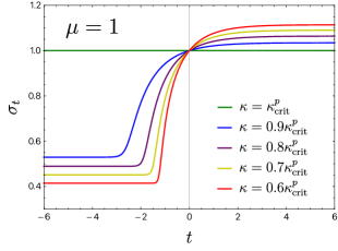
When considering pairs such that , it turns out that . Sticking to these values of , one notices that there exist and such that . Since the vanishing of implies the vanishing of , we conclude that all solutions to Equation (2.10) with are well-defined for all times , satisfying that and . Therefore, they define eternal and regular (in the sense that they asymptote to finite values as ) flows, which do not exist for the Ricci flow case . Some solutions of this type are illustrated in Figure 1 (left).
-
•
For pairs such that , a more detailed examination is required:
-
–
If is greater than the unique real and positive solution of the algebraic equation111This equation is obtained after setting , imposing and identifying . , then all solutions are seen to collapse at finite time. This is due to the fact that , while decreases as goes to zero (so that approaches zero at some finite time).
-
–
Otherwise, there is an interval for which the solution is seen to exist for all times (diverging nonetheless as , while remaining finite for ), thus yielding an eternal flow. The value can be found by solving the equations:
for . If , then solutions collapse at finite time.
On the other hand, if and , the solution is seen to collapse at finite time, while for we have that . Finally, for , if we have that the flow is eternal, diverging as and remaining finite as , while it collapses at finite time if (the case corresponds to the static one).
-
–
2.5.2. Flat homothety flows
In this case, it is possible to find an explicit solution to Equation (2.11). Assuming and defining , the solution can be seen to be:
| (2.13) |
where we have used the Lambert W function (introduced in Remark 2.10). It can be easily checked that for the corresponding solution exists for all times (for strictly positive, it tends to as and grows indefinitely as ), while for the solution is only defined in the interval , where . In this latter case, the solution also asymptotes to as .
On the other hand, if the only solution corresponds to the static one, namely , whereas for the solution reads . The latter is defined for .
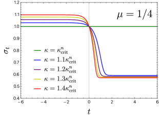
2.5.3. Negative homothety flows
In analogy with the positive case, it is not possible to find explicit solutions for generic , so we restrict ourselves to a qualitative and numerical study of the solutions of Equation (2.12). We define:
We start by examining the existence of static solutions. Demanding , we find:
We note that for , with , there are no static solutions, since would be negative. This suggests to split our study depending on the value of :
-
•
If , there are two different subcases to consider:
-
–
If , we have that , with growing monotonically as we increase and diverging as . Also, we observe that there exists a value such that . Therefore, solutions in this case are eternal and tend to a finite and positive value as and diverge as . The case corresponds to the static solution .
-
–
If , then . Furthermore, it is verified that there always exist and such that . Consequently, these solutions are eternal and regular flows satisfying that and . We show some instances of these solutions in Figure 1 (right).
-
–
-
•
If , regardless of the value of we observe the same qualitative behaviour: the subsequent solution exists for all times, asymptoting to a finite value as and diverging as . This is due to for every and to the existence of such that .
-
•
Finally, for , two subcases need to be addressed:
-
–
For , we have that for , always existing such that . Therefore, the subsequent solutions are defined for all times, remaining finite as and diverging when . The case corresponds to the static solution .
-
–
If , it is easily verified that . Since decreases monotonically as takes smaller values and diverges when , we conclude that these solutions collapse at finite time.
-
–
For , the flow collapses at finite time regardless the value of (if , then ). Finally, if , it is observed that the solution collapses at finite time if , it corresponds to the static one for and it yields a solution that asymptotes to a finite and positive number for and diverges as for .
3. Heterotic supergravity with trivial gauge bundle
The notion of Heterotic soliton was introduced in [39] as a manifold equipped with a solution to the bosonic sector of Heterotic supergravity with trivial gauge bundle at first order in the string slope parameter, which we called the Heterotic soliton system. In the following, we revisit the Heterotic soliton system and discuss some of its basic geometric properties.
3.1. The Heterotic soliton system
Heterotic solitons are expected to be solitons for the Heterotic-Ricci flow, an expectation that we will prove to be correct in the three-dimensional case considered in Section 4, and hence are expected to define a subclass of Heterotic-Ricci solitons for which there exists an interpretation within the context of supergravity.
Definition 3.1.
Let be a non-negative real constant. The Heterotic soliton system on a manifold is the following system of partial differential equations:
| (3.1) |
together with the Bianchi identity:
| (3.2) |
for triples , where is a Riemannian metric on , is a closed one-form and is a three-form. A Heterotic soliton is a triple satisfying the Heterotic soliton system.
Remark 3.2.
Evidently, the Bianchi identity (3.2) is not an identity but an equation that needs to be solved. The terminology comes from the physics community and is nowadays pervasive also in the mathematics community.
We will denote the configuration space and solution space of the Heterotic soliton system by and , respectively. Given , the cohomology class determined by will be called the Lee class of the configuration. This terminology is inherited from [25] in the context of the twisted Hull-Strominger system, for which is necessarily the Lee form of a Hermitian structure on a complex manifold. By the explicit form of Equations (3.1) and (3.2), which are completely determined by supersymmetry, it is clear that the Heterotic soliton system can be considered to be a natural differential system for Riemannian geometries with torsion.
Remark 3.3.
The Heterotic soliton system corresponds to the equations of motion of bosonic Heterotic supergravity with trivial gauge bundle at first order in the string slope parameter [4, 5]. The symmetric part of the first equation in (3.1) is usually referred to in the literature as the Einstein equation, whereas its skew-symmetric part is usually called the Maxwell equation. On the other hand, the second equation in (3.1) is commonly referred to in the literature as the dilaton equation.
A Heterotic soliton for which both and vanish identically reduces to a Ricci-flat metric. Hence, we will refer to such Heterotic solitons as Ricci-flat. If is, in addition, flat, we will say that such a soliton is trivial. A soliton with is a particular instance of steady generalized Ricci soliton [26] which is Ricci-flat if and only if is an exact one-form. Hence, non-Ricci-flat Heterotic solitons with are particular cases of non-gradient steady generalized Ricci solitons. In the following, we will always assume that . For further reference, we introduce the following maps based on the defining equations of the Heterotic soliton system:
| (3.3) |
which we interpret as smooth maps of Fréchet manifolds. Clearly, the solution space of the system corresponds to the preimage of zero by . We incidentally note that very little is known about the structure and properties , our main conjecture being that it should be a finite-dimensional smooth manifold locally around an irreducible solution , namely a solution of the system with no automorphisms.
Remark 3.4.
For every the symmetric and skew-symmetric projections and of are explicitly given by:
These formulas can be very convenient to do explicit computations.
Due to the fact that we are studying an exact truncation of Heterotic supergravity at first order in the string slope parameter, the divergence of the Einstein equation evaluated on an element satisfying the remaining equations of the system may not vanish identically, as we proceed to show below through a calculation that will naturally lead us to introduce the notion of strong Heterotic soliton, see Definition 3.8.
Lemma 3.5.
The following identity holds:
for every , where is the formal adjoint of with respect to the determinant norm and is the formal adjoint of .
Proof.
We choose an orthonormal frame parallel with respect to at a given point . For every parallel with respect to at we compute (using from now on Einstein’s summation convention on repeated indices):
where denotes here the sum over all cyclic permutations of the set . Using now the second Bianchi identity for connections with torsion we obtain after some tedious but straightforward computation:
and we conclude. ∎
We will also need the following:
Lemma 3.6.
The following identity holds for every configuration :
where is a vector field.
Proof.
We choose an orthonormal frame adapted to at a given point and compute:
where is any vector field adapted to at . ∎
Proposition 3.7.
The following formula holds:
for every and .
Proof.
Let . First, recall the standard identities:
for every vector field . On the other hand, a quick computation reveals that:
as well as:
Hence:
which gives the equation in the statement. ∎
Clearly, by the previous proposition, every Heterotic soliton satisfies:
for every vector field . This motivates the following definition.
Definition 3.8.
The strong Heterotic soliton system is the Heterotic soliton system for triples together with the strong condition:
| (3.4) |
A strong Heterotic soliton is a solution of the strong Heterotic soliton system.
The strong Heterotic soliton system is an overdetermined system of partial differential equations. Despite being overdetermined, as we will see below it still has natural non-trivial solutions. This is a remarkable fact that can be traced back to the internal consistency and coherence of supersymmetric field theories and, in particular, Heterotic supergravity and its various truncations. Discussing the consistency of the perturbative expansion Heterotic supergravity and its consistent truncations is beyond the scope of this article. The interested reader is referred to [34] and its references for more details.
Remark 3.9.
Note that every satisfying , and together with the strong condition automatically satisfies:
Identities of this type, involving the divergence of the Einstein equation, are closely related to the existence of variational principles associated with the Heterotic soliton system. Studying the action functionals that can be associated with the Heterotic soliton system is a fundamental problem that is currently a work in progress and that we will consider elsewhere.
The strong condition is an equation in . Hence, by projecting to we obtain an equation in that is satisfied by any strong Heterotic soliton and does not explicitly involve any curvature operators. On the other hand, by contraction we obtain an equation on .
Proposition 3.10.
Let be a solution to the strong condition. Then, the following equations hold:
| (3.5) |
where is any local orthonormal frame.
Proof.
Let be any tangent vector. By (2.1) and the first Bianchi identity for , the totally skew-symmetric part of is explicitly given by:
We choose the local orthonormal frame to be -parallel at some point . Taking in the above formula, differentiating with respect to and summing over , the skew-symmetric part of at can be computed as follows::
where we have used that:
3.2. Lift to the frame bundle
We have introduced the Heterotic soliton system as a system of differential equations for a metric connection with skew-symmetric torsion that is determined by Heterotic supergravity and implicitly by the expected structure of the self-similar solutions to the Heterotic-Ricci flow. In the following, we show that the Heterotic soliton system, and especially its strong condition, can be naturally interpreted when lifted to the reference frame bundle of the underlying manifold . For this, we will adapt the construction of [2, Proposition 7.1] to our case in which the gauge bundle is not an abstract bundle and the gauge connection is not an arbitrary connection but metric-compatible for each choice of Riemannian metric.
Given , we denote by the bundle of oriented frames of . Given any metric connection on , in particular , we denote by:
its Chern-Simons form, which defines a three-form on the total space of . There is a natural map:
from into the Riemannian metrics over that, to every , associates the metric:
where is the metric connection , understood as a one-form in the total space of with values in . In particular, for every we have . Note that the metric is invariant under the principal bundle action of .
Proposition 3.12.
[2, Proposition 7.1] A triple is a strong Heterotic soliton with constant if and only if the associated triple satisfies:
| (3.6) |
where and .
Remark 3.13.
The interest of the previous proposition is that equations (3.6) precisely correspond to the equations of motion of NS-NS supergravity for a pseudo-Riemannian metric of split signature and a three-form flux belonging to a given string class [50] for each choice of metric. The fact that the signature of the metric on the total space of is of split signature is not accidental and can be traced back to the sign of the higher order curvature term in (3.1), see also Remark 2.11. Had this term appeared with the opposite sign (recall that is assumed to be non-negative), then the corresponding would be positive definite. This would be however inconsistent with the physical interpretation of the system.
4. Heterotic solitons on three-manifolds
In this section, we consider the Heterotic soliton system on a compact three-manifold with the goal of obtaining a classification result for three-dimensional strong Heterotic solitons.
4.1. Three-dimensional reformulation
The Heterotic soliton system can be simplified in three dimensions using the fact that the Hodge dual of is a function and the fact that the Riemann tensor is completely determined by the Ricci curvature. Given a triple , we write in terms of the unique function , where denotes the Riemannian volume form associated to . Consequently, we define the configuration space of the Heterotic soliton system on as the set of triples , where is a Riemannian metric, is a one-form and is a function. Similarly, we define the set of Heterotic solitons on as the set of triples such that satisfies the Heterotic soliton system with parameter .
Using the Lemma A.1 in Appendix A we can write the Heterotic system in three dimensions as a system of differential equations for a metric , a closed one-form and a function involving the Ricci tensor and scalar curvature of as the only curvature operators.
Proposition 4.1.
A triple is a Heterotic soliton if and only if it satisfies the following system of equations:
| (4.1) | |||
| (4.2) |
where .
Proof.
Since in three dimensions the Bianchi equation (2.2) is automatically satisfied, a triple is a Heterotic soliton if and only if satisfies equations (3.1). Plugging Equation (A.1) into and using the identity:
Therefore, the Heterotic soliton system, as introduced in Definition 4.2, is equivalent in three dimensions to equations (4.1) and (4.2) for tuples of the form .
Definition 4.2.
The following result is the key reason why solutions to the three-dimensional Heterotic system are relevant in relation to the three-dimensional Heterotic-Ricci flow: the former are, as their name suggests, self-similar solutions of the latter.
Proposition 4.3.
Let be a three-dimensional Heterotic soliton. Then, there exists a one-parameter family of diffeomorphisms for some interval such that:
is a Heterotic-Ricci flow.
Proof.
Suppose that and define the one-parameter family of diffeomorphisms defined by the flow of . Then:
where we have used that is closed. Plugging this equation into (2.7) we directly obtain (4.1). Regarding (2.7), we compute:
Here we have used that , which implies:
together with the identity . Hence is a solution of the three-dimensional Heterotic-Ricci flow and consequently solutions of (4.1) and (4.2) are self-similar solutions of the Heterotic-Ricci flow. ∎
Remark 4.4.
We expect Heterotic solitons in all dimensions to be actual solitons for the Heterotic-Ricci flow. However, in dimensions larger than four, is in general not closed, and therefore obtaining the solitons of the flow requires a precise understanding of the symmetries of the system when formulated either on a string structure [33, 50, 62] or or on a transitive Courant algebroid [2, 20], see Remark 2.6. We plan to come back to this issue in the future.
4.2. General properties
In this subsection, we will prove a number of structural results about three-dimensional Heterotic solitons.
Proposition 4.5.
Let be a closed Riemannian three-manifold. A three-dimensional Heterotic soliton is trivial if and only if .
Proof.
The only if direction holds by definition. Therefore, assume that . The trace of Equation (4.1) reduces to:
where is the trace-free part of the Ricci tensor. On the other hand, the second equation in (4.1) reduces to:
Combining the previous equations and integrating we obtain:
where is the volume form of . Hence , so is Ricci-flat. Since is three-dimensional implies that is in fact a flat Riemannian metric. ∎
Lemma 4.6.
Let be a non-trivial three-dimensional Heterotic soliton. Then, there exists a function such that and for a non-zero constant .
Proof.
Let be a non-trivial three-dimensional Heterotic soliton. We first prove that is nowhere vanishing. To do this, assume that for a given . For every smooth curve:
where is an interval containing and , the first equation in (4.2) implies:
which is a linear ordinary differential equation for . Since , the existence and uniqueness of solutions to the previous ordinary differential equation imply that for all . Since this holds for every such and is connected, we conclude that vanishes identically, which is not allowed since is by assumption a non-trivial Heterotic soliton, cf. Proposition 4.5. Hence is nowhere vanishing, in which case the first equation in (4.2) is equivalent to and for and for a non-zero constant . ∎
By the previous proposition, we will always assume from now on that for any non-trivial three-dimensional Heterotic soliton . This allows us to denote three-dimensional Heterotic solitons simply as pairs . In particular, we will sometimes refer to as the dilaton of the three-dimensional Heterotic soliton .
Proposition 4.7.
Let be a non-trivial Heterotic soliton. Then, the scalar curvature of is strictly negative on some non-empty open set of .
Proof.
Let be a Heterotic soliton and consider the second equation in (4.2), which can be equivalently rewritten as follows:
where denotes the Hessian of with respect to . If is constant then the previous equation reduces to , which immediately implies that is a strictly negative constant since cannot be zero. If is non-constant then evaluating the previous equation at an absolute minimum of we obtain:
where the subscript denotes evaluation at . Since is an absolute minimum and is strictly positive, we have and we conclude. ∎
Remark 4.8.
The previous proposition rules out the possibility of having three-dimensional Heterotic solitons with positive scalar curvature, which in dimension three is obstructed [32]. In contrast, any function on that is negative on some open set is the scalar curvature of a metric on .
Given the complexity of the Heterotic soliton system, it is natural to look for examples that satisfy natural curvature conditions. In the following result, we consider metrics whose Ricci tensor has constant principal curvatures, where the latter are defined as the eigenvalues of the Ricci endomorphism.
Proposition 4.9.
A non-trivial three-dimensional Heterotic soliton with constant dilaton has constant principal Ricci curvatures which satisfy one of the following conditions:
-
(1)
and .
-
(2)
and . In particular, the universal cover of is isometric to either or equipped with a left-invariant metric.
-
(3)
and . In particular is a hyperbolic three-manifold endowed with a metric of scalar curvature .
Proof.
Assume that is a constant, which by Proposition 4.5 must then be non-zero. With this assumption, Equations (4.1) and (4.2) reduce to:
Taking the trace of the first equation and combining it with the second equation we find:
which plugged back into the previous equations yields:
| (4.3) |
The discriminant of the previous equation can be verified to be one, and by solving it we obtain the cases listed in the statement of the Proposition, similarly to [39, Proposition 4.6 and Theorem 4.9], whose proof involves solving the same algebraic equation for the Ricci tensor. ∎
Remark 4.10.
In case of the previous proposition, Reference [39] proves the existence of an associated Sasakian structure, possibly involving a different Riemannian metric, constructed out of the unit-norm eigenvector of with positive eigenvalue. Very little is currently known about the basic properties of this auxiliary Sasakian structure.
Ideally, we would like to construct or, at least, prove the existence of three-dimensional Heterotic solitons with non-constant dilaton . The following result excludes for this purpose the case of Heterotic solitons with Einstein metrics.
Theorem 4.11.
All Einstein three-dimensional Heterotic solitons have constant dilaton.
Proof.
If is Einstein, so that , the Einstein equation (4.1) becomes:
| (4.4) |
Taking the trace with respect to in this equation yields:
| (4.5) |
Using now the dilaton equations (4.2) we readily obtain , for some explicit rational function given by:
Applying then (4.4) to (the metric dual of) and using that:
we obtain:
| (4.6) |
Since and , we deduce from (4.6) that , where is some (explicit) non-vanishing polynomial. This shows that the dilaton is constant. ∎
If we weaken the condition of having constant principal Ricci curvatures in order to construct Heterotic solitons with non-constant dilaton we can rapidly encounter important obstructions, as illustrated by the following result.
Proposition 4.12.
Let be a non-trivial three-dimensional Heterotic soliton such that and:
Then is diffeomorphic to the sphere .
Proof.
Suppose is a Heterotic soliton with non-constant dilaton . We evaluate Equations (4.1) and (4.2) at a critical point of whose critical value we denote by . We obtain:
Taking the trace of the first equation and combining it with the second we obtain a quadratic equation for whose coefficients are constant due to the assumption and . Hence, the function can have at most two critical values, implying that it is either constant, which is not allowed, or has exactly two critical points. The latter implies that is diffeomorphic to the sphere [38, 51]. ∎
We note that the existence of three-dimensional Heterotic solitons with non-constant dilaton is currently an open problem.
4.3. Classification of three-dimensional strong Heterotic solitons
In this subsection, we consider strong three-dimensional Heterotic solitons and provide their complete classification.
Lemma 4.13.
A strong three-dimensional Heterotic soliton has constant dilaton .
Proof.
Every strong Heterotic soliton satisfies by definition the strong condition (3.4) and therefore also satisfies its skew-symmetric projection (3.5). Plugging into equation (3.5) and simplifying we obtain that it is equivalent to:
Setting now in the previous equation we obtain that it is equivalent to:
Integrating over , this implies . ∎
The previous lemma reduces the study of three-dimensional strong Heterotic solitons to the study of the strong condition given at Equation (3.4) in the three possible classes of three-dimensional Heterotic solitons listed in Proposition 4.9. Since is a non-zero constant, the system (4.1)–(4.2) is equivalent to (4.3) and the strong equation (3.4) becomes:
| (4.7) |
We easily compute for every tangent vectors , therefore using the Bianchi identity we obtain after a straightforward computation that (4.7) is equivalent to:
| (4.8) |
where is the traceless Ricci tensor. If is Einstein, this equation is clearly satisfied, so the solitons in case (3) of Proposition 4.9 satisfy automatically the strong condition. If is of type (1) or (2) of Proposition 4.9, the Ricci tensor has one double eigenvalue and one simple eigenvalue . Let denote a unit vector field on satisfying (here we might have to replace with a double cover in order for to be globally defined). We write:
so . The strong equation (4.8) becomes:
For this gives . Reinjecting in the above equation we obtain:
Taking the interior product with in this equation and using again yields:
showing that for every . In particular, is Killing. The Bochner formula gives whence , that is, . We are thus in case (1) of Proposition 4.9. Reversing the order of the above calculations shows that, conversely, if the Ricci tensor of satisfies the condition (1) in Proposition 4.9 and is a unit length vector field on satisfying , then is a strong three-dimensional soliton. It remains to characterize the manifolds satisfying these conditions.
Proposition 4.14.
Let be a complete simply connected three-dimensional Riemannian manifold such that there exists a positive constant and a unit vector field with and . Then is isometric to the Heisenberg group , endowed with a left-invariant metric. Conversely, for every left-invariant metric on there exist and with the above properties.
Proof.
Consider the metric connection with torsion on defined by
We have
so is -parallel. A straightforward but tedious computation then shows that is flat. Consequently, there exists a -parallel oriented orthonormal frame on . We have:
and similarly . This shows that the frame satisfies the commutator relations
of the Heisenberg Lie algebra , and thus is isometric to endowed with the left-invariant metric determined by the scalar product .
Conversely, if is a positive constant and is the Heisenberg group endowed with the above left-invariant metric, the standard formulas of Riemannian Lie groups show that the unit left-invariant vector field induced by satisfies and that . ∎
Altogether, the previous discussion results in the following classification of compact strong Heterotic solitons in three dimensions.
Theorem 4.15.
Every compact three-dimensional strong Heterotic soliton has constant dilaton and is either isometric to a compact quotient of the Heisenberg group equipped with a left-invariant metric or homothetic to a compact hyperbolic three-manifold.
5. Rigidity of Einstein Heterotic solitons
All known Heterotic solitons on a compact three-manifold have constant principal Ricci curvatures and constant dilaton . In this section, we study the local moduli of three-dimensional Heterotic solitons around an Einstein Heterotic soliton, which must be then either flat or of negative constant sectional curvature, in order to evaluate the possibility of deforming them to construct compact three-dimensional Heterotic solitons with non-constant dilaton. For definiteness, we will exclusively focus on the deformation of non-trivial Heterotic solitons with constant dilaton. The deformation problem of trivial Heterotic solitons can be easily studied by directly inspecting the Heterotic soliton system, from which the rigidity of trivial Heterotic solitons follows.
In three dimensions the Bianchi identity is automatically satisfied and, after solving the Maxwell equation as prescribed in Lemma 4.6 the maps introduced in (3.3) reduce to:
namely to the maps defined by the Einstein and dilaton equations. The diffeomorphism group acts naturally on . This action is smooth in the Fréchet category when we consider as a Fréchet manifold and as a Fréchet-Lie group. Furthermore, the map is diffeomorphism-equivariant, namely:
for every and . Hence, the action maps Heterotic solitons to Heterotic solitons. The moduli space of three-dimensional Heterotic solitons on a closed three-manifold is then defined as follows:
It is equipped with the quotient topology of the subspace topology induced by the topology of corresponding to its Fréchet manifold structure. The main result that we need to understand the local structure of is a slice theorem for the action of on .
5.1. Local slice in configuration space
The fact that we are studying Heterotic solitons in three dimensions together with the simplification given by Lemma 4.6, implies that the configuration space of the system reduces in this case to that of the classical Ricci solitons, namely pairs as described above, although the equations that define our system are remarkably more complicated than the standard Ricci soliton system. Furthermore, for us is a variable of the system whereas in the theory of Ricci solitons is usually considered as being completely determined as an eigenvalue of a Schrödinger type of operator associated to the system. The moduli space of standard Ricci solitons together with a slice theorem for the corresponding action of the diffeomorphism group is proved in [46] by considering Sobolev completions of the spaces involved. Here we adopt a direct approach and we consider the smooth right action of on via pull-back. For every define:
to be the orbit map associated with . In particular, is the orbit of the action passing through . The differential of at the identity reads:
where the symbol denotes the Lie derivative. Its adjoint is given by:
Lemma 5.1.
We have a orthogonal decomposition:
in terms of closed subspaces of .
Proof.
The result follows from the fact that the symbol of is injective. ∎
Therefore, if is a three-dimensional Einstein Heterotic soliton with constant dilaton, then the projection of to is zero and the slice for the action of around can be characterized as follows.
Proposition 5.2.
Let be a three-dimensional Einstein Heterotic soliton with constant dilaton. Any smooth submanifold of the form:
where is a slice for the action of on is a slice for the action of on . In particular:
is the tangent bundle of at .
Remark 5.3.
Thanks to recent developments in the theory of infinite dimensional groups and actions [10] we do not need to work in any Sobolev completion of and we can remain in the category of Fréchet spaces and Fréchet Lie groups of smooth sections.
5.2. Essential deformations
Let be a non-trivial three-dimensional Einstein Heterotic soliton with constant dilaton. Recall that in this case, the Heterotic soliton system implies:
We will tacitly use these equations in the following. The existence of a natural slice for the action of the diffeomorphism group around every point immediately implies the following inclusion of vector spaces:
where the tangent space of at the class determined by and:
is the differential of at . This motivates the following definition.
Definition 5.4.
Let be a non-trivial three-dimensional Einstein Heterotic soliton with constant dilaton. The vector space of essential deformations of is:
If then is rigid.
Remark 5.5.
By the existence of a slice around , the previous notion of rigidity corresponds to the intuitive one, namely, if is rigid then there exists a neighborhood of in in which every element is diffeomorphic to .
Lemma 5.6.
Let be a non-trivial three-dimensional compact Einstein Heterotic soliton with constant dilaton. Then, the following equation holds:
for every .
Proof.
Let be a three-dimensional Einstein Heterotic soliton with a constant dilaton and fix a pair . We have:
which follow from the standard formulas for the linearization of the Ricci and scalar curvatures [6] and Equation (A.1) in Appendix A. Note that the latter implies in particular:
Using the previous formulae we compute:
In particular:
Assuming now that holds, the differential of the trace of the Einstein equation (4.1) at gives:
On the other hand, the differential of equation (4.2) at immediately gives:
Combining the previous two equations we obtain:
and a quick computation reveals that:
whence:
and we conclude. ∎
Remark 5.7.
By the previous lemma, if then:
We will tacitly use these identities in the following.
Lemma 5.8.
Let be a non-trivial three-dimensional compact Einstein Heterotic soliton with constant dilaton. Then, the following equations hold:
for every .
Proof.
Theorem 5.9.
Let be a non-trivial three-dimensional compact Einstein Heterotic soliton with constant dilaton. Then .
Proof.
Fix a non-trivial three-dimensional compact Einstein Heterotic soliton with constant dilaton and a pair . Denote by the exterior covariant derivative defined by the Levi-Civita connection of on the bundle of one-forms taking values in . Denote by its formal adjoint. Our starting point is the celebrated Weitzenböck formula:
where , and is the linear operator given explicitly by:
in terms of an orthonormal basis . We compute:
where is the trace-free part of and we have used that:
We obtain:
upon use of Lemma 5.8. We apply now to both sides of the previous equation. Observing that the result of applying to each monomial in the previous equation is a constant times and that the combination of all terms does not vanish we conclude:
which in turn implies since and by assumption. Hence, by Lemma 5.6 we also have and by Lemma 5.8 we finally end up with:
This immediately implies since the differential operator of the left hand side of the equation is positive. ∎
The existence of a slice for the action of the diffeomorphism group around together with the previous theorem immediately implies the following result.
Corollary 5.10.
Three-dimensional compact Einstein Heterotic solitons with constant dilaton are rigid.
Remark 5.11.
We are not aware of any rigidity result for a compact solution of a supergravity theory, especially in the non-supersymmetric case.
Appendix A Riemannian curvature in three dimensions
Let be a Riemannian three-manifold. The Riemannian tensor of can be written as follows in terms of its Ricci tensor :
| (A.1) |
where is the scalar curvature of . In particular, using the previous formula it is easy to show that the contraction , is given by:
| (A.2) |
where we have defined:
In particular, the norm of is given by:
Using the previous formulae, we can obtain an explicit expression for in terms of standard curvature tensors of and derivatives of .
Lemma A.1.
Let be a Riemannian metric on and . The following equation holds:
| (A.3) |
where we have set .
Remark A.2.
Here denotes the standard commutator of endomorphisms, understanding both and as endomorphisms of by means of the musical isomorphisms determined by .
Proof.
Since , we have:
Using the previous formula we compute:
Substituting this expression into and expanding we obtain (A.1) and we conclude. ∎
Using the previous lemma we can compute one-half of the trace of , which corresponds to twice the norm of , obtaining:
This formula is tacitly used in several computations throughout the paper.
References
- [1] T. Aubin, Some Nonlinear Problems in Riemannian Geometry, (Springer monographs in mathematics, 1998.
- [2] D. Baraglia and P. Hekmati, Transitive Courant Algebroids, String Structures and T-duality, Adv. Theor. Math. Phys. 19 (2015), 613.
- [3] K. Becker, M. Becker and J. H. Schwarz, String Theory and M-Theory: A Modern Introduction, Cambridge University Press, 2006.
- [4] E. Bergshoeff and M. de Roo, Supersymmetric Chern-Simons Terms in Ten-dimensions, Phys. Lett. B 218 (1989), 210.
- [5] E. Bergshoeff and M. de Roo, The Quartic Effective Action of the Heterotic String and Supersymmetry, Nucl. Phys. B 328 (1989), 439.
- [6] A. L. Besse, Einstein Manifolds, Springer 1987.
- [7] J. Buckland, Short-time existence of solutions to the cross curvature flow on 3-manifolds, Proceedings of the AMS 134 no. 6, (2005), 1803–1807.
- [8] M. Carfora and C. Guenther, Scaling and Entropy for the RG-2 Flow, Commun. Math. Phys. 378 (2020), 369–399.
- [9] H.-D. Cao, Geometry of Ricci solitons, Chin. Ann. Math. 2006, 27B, 121–142.
- [10] T. Diez and G. Rudolph, Slice theorem and orbit type stratification in infinite dimensions, Differential Geometry and its Applications, 65 (2019), 176 – 211.
- [11] T. Fei, A Construction of Non-Kähler Calabi-Yau Manifolds and New Solutions to the Strominger System, Advances in Mathematics 302 (2016), 529–550.
- [12] T. Fei, B. Guo and D. H. Phong, Parabolic Dimensional Reductions of 11D Supergravity, Commun. Math. Phys. 369 (2019), 811–836.
- [13] T. Fei, D. H. Phong, S. Picard and X. Zhang, Geometric Flows for the Type IIA String, arXiv:2011.03662.
- [14] T. Fei, D. H. Phong, S. Picard and X. Zhang, Estimates for a geometric flow for the Type IIB string, Math. Ann. 382, 1935–1955 (2022).
- [15] T. Fei and S. T. Yau, Invariant Solutions to the Strominger System on Complex Lie Groups and Their Quotients, Commun. Math. Phys. 338 (2015), 1183–1195.
- [16] M. Fernández, S. Ivanov, L. Ugarte and R. Villacampa, Non-Kähler heterotic-string compactifications with non-zero fluxes and constant dilaton, Commun. Math. Phys. 288 (2009) 677–697.
- [17] M. Fernández, S. Ivanov, L. Ugarte and D. Vassilev, Non-Kähler heterotic string solutions with non-zero fluxes and non-constant dilaton, JHEP 6 (2014) 73.
- [18] J. X. Fu, L. S. Tseng and S. T. Yau, Local heterotic torsional models, Commun. Math. Phys. 289 (2009) 1151–1169.
- [19] J. X. Fu and S. T. Yau, The theory of superstring with flux on non-Kähler manifolds and the complex Monge-Ampère, J. Differ. Geom. 78 (2008) 369–428.
- [20] M. García-Fernández, Ricci flow, Killing spinors, and T-duality in generalized geometry, Adv. Math. 350 (2019), 1059–1108.
- [21] E. García-Río, R. Mariño-Villara, M. E. Vázquez-Abal and R. Vázquez-Lorenzo, Fixed points and steady solitons for the two-loop renormalization group flow, J. Fixed Point Theory Appl. Accepted.
- [22] M. García-Fernández and R. Gonzalez Molina, Harmonic metrics for the Hull-Strominger system and stability, preprint arXiv:2301.08236.
- [23] M. García-Fernández and R. Gonzalez Molina, Futaki Invariants and Yau’s Conjecture on the Hull-Strominger system, preprint arXiv:2303.05274.
- [24] M. Garcia-Fernández, J. Jordan, and J. Streets, Non-Kähler Calabi-Yau geometry and pluriclosed flow, preprint arXiv:2106.13716.
- [25] M. García-Fernández, R. Rubio, C. Shahbazi and C. Tipler, Canonical metrics on holomorphic Courant algebroids, Proc. Lond. Math. Soc. 125 no.3 (2022), 700–758.
- [26] M. García-Fernández and J. Streets, Generalized Ricci Flow, AMS University Lecture Series, 2021.
- [27] K. Gimre, C. Guenther, and J. Isenberg, A geometric introduction to the two-loop renormalization group flow, J. Fixed Point Theory Appl., 14 (2013), 3–20.
- [28] K. Gimre, C. Guenther and J. Isenberg, Short-time existence for the second order renormalization group flow in general dimensions, Proc. Amer. Math. Soc. 143 (2015), 4397–4401.
- [29] D. Glickenstein, L. Wu, Soliton metrics for two-loop renormalization group flow on 3D unimodular Lie groups, J. Fixed Point Theory Appl. 19, 1977–1982 (2017).
- [30] R. Hamilton, Three-manifolds with positive Ricci curvature, J. Differ. Geom. 17 (1982), 255–306.
- [31] C. Hull, Compactifications of the Heterotic Superstring, Phys. Lett. B 191 (1986) 357–364.
- [32] J. Kazdan and F. Warner, Scalar curvature and conformal deformation of Riemannian structure, J. Differ. Geom. 10 (1975), 113–134.
- [33] T. P. Killingback, World-sheet anomalies and loop geometry, Nuclear Phys. B 288 (1987), 578–588.
- [34] I. V. Melnikov, R. Minasian and S. Sethi, Heterotic fluxes and supersymmetry, JHEP 6 (2014), 174.
- [35] R. R. Metsaev and A. A. Tseytlin, Two loop beta function for the generalized bosonic sigma model, Phys. Lett. B 191 (1987), 354–362.
- [36] R. R. Metsaev and A. A. Tseytlin, Order alpha-prime (Two Loop) Equivalence of the String Equations of Motion and the Sigma Model Weyl Invariance Conditions: Dependence on the Dilaton and the Antisymmetric Tensor, Nucl. Phys. B 293 (1987), 385–419.
- [37] J. Milnor, Curvatures of Left Invariant Metrics on Lie Groups, Adv. Math. 21 (1976), 293–329.
- [38] J. Milnor, Sommes de variétés différentiables et structures différentiables des sphères, Bull. Soc. Math. de France, 87 (1959), 439 – 444.
- [39] A. Moroianu, Á. Murcia and C. S. Shahbazi, Heterotic solitons on four-manifolds, New York J. Math. 28 (2022), 1463–1497.
- [40] T. A. Oliynyk, The 2nd order renormalization group flow for non-linear sigma models in 2 dimensions, Class. Quant. Grav. 26 (2009), 105020.
- [41] T. Oliynyk, V. Suneeta, and E. Woolgar, A gradient flow for worldsheet nonlinear sigma models, Nuclear Phys. B 739 no. 3 (2006), 441–458. MR 2214659 53, 68, 111, 112.
- [42] D. H. Phong, S. Picard and X. Zhang, New curvature flows in complex geometry, Surveys in Differential Geometry 22 (2017).
- [43] D. H. Phong, S. Picard, and X. Zhang, Anomaly flows, Communications in Analysis and Geometry Volume 26, Number 4, 955–1008, 2018.
- [44] D. H. Phong, S. Picard, and X. Zhang, The Anomaly flow and the Fu-Yau equation, Ann. PDE 4, 13 (2018).
- [45] D. H. Phong, Geometric flows from unified string theories, Contribution to Surveys in Differential Geometry, ”Forty Years of Ricci flow”, edited by H.D. Cao, R. Hamilton, and S. T. Yau.
- [46] F. Podestà and A. Spiro , On Moduli Spaces of Ricci Solitons, J. Geom. Anal. 25 (2015), 1157-–1174.
- [47] J. Polchinski, String theory. Vol. 1: An introduction to the bosonic string, Cambridge Monographs on Mathematical Physics (1998).
- [48] J. Streets, Regularity and expanding entropy for connection Ricci flow, J. Geom. Phys. 58 no. 7 (2008), 900–912. MR 2426247 68, 87, 118.
- [49] A. Strominger, Superstrings with torsion, Nucl. Phys. B274 (2) (1986), 253–284.
- [50] C. Redden, String structures and canonical 3-forms, Pacific J. Math. 249 (2011) 447–484.
- [51] R. H. Rosen, A weak form of the star conjecture for manifolds, Notices Amer. Math. Soc. 7 (1960), 380. Abstract 570–28.
- [52] P. Ševera and F. Valach, Courant Algebroids, Poisson Lie T-Duality, and Type II Supergravities, Commun. Math. Phys. 375 (2020) no. 1, 307–344.
- [53] J. Streets, Generalized geometry, T-duality, and renormalization group flow, Journal of Geometry and Physics Volume 114, 2017, 506–522.
- [54] J. Streets, Generalized Kähler Ricci flow and the classification of nondegenerate generalized Kähler surfaces, Adv. Math. 316 (2017), 187–215.
- [55] J. Streets, Classification of solitons for pluriclosed flow on complex surfaces, Math. Ann., 375(3-4):1555–1595, 2019.
- [56] J. Streets, Scalar curvature, entropy, and generalized Ricci flow, preprint arXiv:2207.13197.
- [57] J. Streets and G. Tian, A parabolic flow of pluriclosed metrics, Int. Math. Res. Not. IMRN, (16): 3101–3133, 2010.
- [58] J. Streets and G. Tian, Regularity results for pluriclosed flow, Geom. Topol. 17(4): 2389–2429, 2013.
- [59] J. Streets and G. Tian, Generalized Kähler geometry and the pluriclosed flow, Nuclear Phys. B 858, 366–376, 2012.
- [60] J. Streets and Y. Ustinovskiy, Classification of generalized Kähler-Ricci solitons on complex surfaces, Communications on Pure and Applied Mathematics, 2020.
- [61] J. Streets and Y. Ustinovskiy, The Gibbons-Hawking ansatz in generalized Kähler geometry, Communications in Mathematical Physics volume 391, 707–778 (2022).
- [62] K. Waldorf, String connections and Chern–Simons theory, Trans. Amer. Math. Soc. 365 (2013), no. 8, 4393–4432.