Uniform approximation of common Gaussian process kernels using equispaced Fourier grids

Abstract

The high efficiency of a recently proposed method for computing with Gaussian processes relies on expanding a (translationally invariant) covariance kernel into complex exponentials, with frequencies lying on a Cartesian equispaced grid. Here we provide rigorous error bounds for this approximation for two popular kernels—Matérn and squared exponential—in terms of the grid spacing and size. The kernel error bounds are uniform over a hypercube centered at the origin. Our tools include a split into aliasing and truncation errors, and bounds on sums of Gaussians or modified Bessel functions over various lattices. For the Matérn case, motivated by numerical study, we conjecture a stronger Frobenius-norm bound on the covariance matrix error for randomly-distributed data points. Lastly, we prove bounds on, and study numerically, the ill-conditioning of the linear systems arising in such regression problems.

1 Introduction

Over the last couple of decades, Gaussian processes (GPs) have seen widespread use in statistics and data science across a range of natural and social sciences [23, 3, 11, 8, 13, 17]. In the canonical Gaussian process regression task, the goal is to recover an unknown real-valued function $f:D\subseteq\mathbb{R}^{d}\to\mathbb{R}$ using noisy observations of that function. Specifically, given data locations $x_{1},\dots,x_{N}\in\mathbb{R}^{d}$, and corresponding observations $y_{1},\dots,y_{N}\in\mathbb{R}$, the usual Gaussian process regression model is

$$y_{n} \;\sim\;f(x_{n})+\epsilon_{n},\qquad n=1,\ldots,N,$$ (1)

$$f(x) \;\sim\;\mathcal{GP}(m(x),k(x,x^{\prime})),$$ (2)

where $\mathcal{GP}$ denotes a Gaussian process distribution, $\epsilon_{n}\sim\mathcal{N}(0,\sigma^{2})$ is independent and identically distributed (iid) noise of known variance $\sigma^{2}>0$, $m:\mathbb{R}^{d}\rightarrow\mathbb{R}$ is a given prior mean function, and $k:\mathbb{R}^{d}\times\mathbb{R}^{d}\to\mathbb{R}$ is a given positive definite covariance kernel [23]. In practice, $k$ is often also translation-invariant, that is, $k(x,x^{\prime})=k(x-x^{\prime})$.

In general, the mean function $m$ can be set to zero by subtraction, which from now we will assume has been done. Then, the marginal posterior of $f$ at any point $x\in D$ is Gaussian with mean $\mu(x)$ and variance $s(x)$ given by,

$$\mu(x) = \sum_{n=1}^{N}\alpha_{n}k(x,x_{n}),$$ (3)

$$s(x) = k(x,x)-\sum_{n=1}^{N}\gamma_{x,n}k(x,x_{n}),$$ (4)

where $\bm{\alpha}:=\{\alpha_{n}\}_{n=1}^{N}$ and $\bm{\gamma}_{x}:=\{\gamma_{x,n}\}_{n=1}^{N}$ are the vectors in $\mathbb{R}^{N}$ that uniquely solve the $N\times N$ symmetric linear systems

$$(K+\sigma^{2}I)\bm{\alpha} = {\mathbf{y}},$$ (5)

$$(K+\sigma^{2}I)\bm{\gamma}_{x} = {{\mathbf{k}}_{x}},$$ (6)

respectively, where $K$ denotes the $N\times N$ positive semidefinite matrix with $K_{i,j}=k(x_{i},x_{j})$, and ${{\mathbf{k}}_{x}}:=\{k(x,x_{n})\}_{n=1}^{N}$. These are known as “function space” linear systems [23].

While GP regression has achieved widespread popularity, an inherent practical limitation of the procedure is its computational cost. A dense direct solution of the above linear systems requires ${\mathcal{O}}(N^{3})$ operations, and in the case of variance $s(x)$ a new right-hand side and solve is needed for each $x$. Since in many modern data sets $N$ can be in the millions or more, a large literature has emerged on faster approximate methods for solving these linear systems, and related tasks such as computing the determinant [22, 20, 23, 12, 32, 1, 19, 4, 7]. An in-depth review of the computational environment for GP regression is outside the scope of this paper, though a summary can be found in, for example, [17, 18, 16].

In this work, we analyze the equispaced Fourier Gaussian process (EFGP) regression approach recently proposed by the authors [16]. Briefly, in EFGP, the covariance kernel is factorized as $k(x-x^{\prime})\approx\tilde{k}(x-x^{\prime}):=\sum_{j=1}^{M}\phi_{j}(x)\phi_{j}(x^{\prime})$ where the plane wave bases $\{\phi_{j}\}$ arise from an equispaced quadrature discretization of the inverse Fourier transform of the covariance kernel, using $M={\mathcal{O}}(m^{d})$ nodes, where $m$ sets the grid size in each dimension. This leads to a rank-$M$ approximation of the covariance matrix $K\approx\tilde{K}=\Phi\Phi^{*}$. The method then proceeds to solve the equivalent “weight space” dual system, with $M\times M$ system matrix $\Phi^{*}\Phi+\sigma^{2}I$, using conjugate gradients (CG) [9]. The method derives its computational efficiency from the ability to rapidly apply the Toeplitz matrix $\Phi^{*}\Phi$ using padded $d$-dimensional fast Fourier transforms (FFTs) with cost $O(M\log{M})$. A precomputation which exploits nonuniform FFTs of cost $O(N+M\log{M})$ is needed; however, the cost per iteration is independent of the number of data points $N$. The result is that for low-dimensional problems (say, $d\leq 3$), $N$ as high as $10^{9}$ can be regressed in minutes on a desktop; this is much faster that competing methods in many settings [16].

Error bounds for such a Fourier kernel approximation are crucial in practice in order to choose the numerical grid spacing $h$ and grid size $m$. Then the error in the computed posterior mean when using $\tilde{k}$ as the covariance kernel can be bounded in terms of the Frobenius norm of $\tilde{K}-K$, which in turn can be bounded by the uniform kernel approximation error [16, Thm. 4.4]. This is a deterministic analysis of what is sometimes termed “computational uncertainty” [31]. This motivates us to derive error estimates for $\tilde{k}-k$, for the commonly-used squared exponential (SE) and Matérn kernels, with explicit dimension- and kernel-dependent constants. Our bounds are uniform over a kernel argument lying in $[-1,1]^{d}$, as appropriate for evaluating the kernel $\tilde{k}(x-x^{\prime})$ for all $x,x^{\prime}$ in the hypercube $D=[0,1]^{d}$. We provide convenient explicit bounds on $h$ and $m$ that guarantee a user-specified uniform error $\varepsilon$ (Corollaries 3 and 6). Our Matérn bounds are reminiscent of an analysis of Gaussian random field sampling by Bachmayr et al. [2], but we include kernel approximation error and our constants are explicit. Since an equispaced tensor-product grid is perhaps the simplest (deterministic) way to discretize a kernel in Fourier space, we expect the bounds to have wider applications to kernel approximations and Gaussian random fields.

Yet, we find that such bounds are in practice pessimistic for Matérn kernels of low smoothness $\nu$, due to the slow algebraic Fourier decay of the kernel. To address this discrepancy we conjecture a stronger bound on $\|\tilde{K}-K\|_{F}$ for data points drawn iid randomly from some absolutely continuous measure. We support this with a brief derivation and a numerical study. This provides a heuristic for choosing more efficient EFGP numerical parameters.

Finally, motivated by experiments [16, Sec. 5] exhibiting very large CG iteration counts, we include a preliminary analysis and study of the condition numbers of the “exact” (true kernel $k$) linear system, and the approximate (kernel $\tilde{k}$) function and weight space systems. While the issue of ill-conditioning of the function space system is well known [26, 24] (and studied in the operator case [29] as well as in the $\sigma=0$ setting of radial basis approximation [30, Ch. 12]), the weight space system condition number is less well studied. It turns out that both function- and weight-space linear systems are nearly as ill-conditioned as their upper bounds allow (about $N/\sigma^{2}$), even though the the GP regression problem itself is very well-conditioned (Proposition 13). It is thus a curious situation from the perspective of numerical analysis to have a well-conditioned problem require an ill-conditioned algorithm for its solution (compare, e.g., the unstable algorithm discussed in [27, Ch. 15]). This twist complements the main kernel error bounds of the paper.

The remainder of this paper is structured as follows. In Section 2, we review bounds on errors in posterior means using approximate GP regression, and provide a summary of the EFGP algorithm introduced in [16]. The main results are the approximation errors for the SE and Matérn kernels derived in Section 3. In Section 4, we conjecture a bound for the norm of $\tilde{K}-K$ in terms of a weighted $L^{2}$ approximation of the covariance kernel, and give a heuristic derivation along with numerical evidence. We discuss bounds on various condition numbers, as well as a numerical study, in Section 5. We summarize and list some open questions in Section 6.

2 Preliminaries

In this section, we motivate the study of the kernel approximation error by reviewing how it controls the error in the posterior mean (relative to exact GP regression with the true kernel). We also summarize the EFGP numerical method. Both are presented in more depth in [16].

2.1 Error estimates for the posterior mean

Suppose that $\tilde{k}$ is an approximation to $k$ with a uniform error $\varepsilon$, i.e.

$$\sup_{x,x^{\prime}\in D}|k(x,x^{\prime})-\tilde{k}(x,x^{\prime})|\leq\varepsilon,$$

then, since all data points lie in $D$, the error in the corresponding covariance matrix is easily bounded by

$$\|K-\tilde{K}\|\leq\|K-\tilde{K}\|_{F}\leq N\varepsilon,$$ (7)

where $\|\cdot\|$ denotes the spectral norm of the matrix, and $\|\cdot\|_{F}$ denotes the Frobenius norm.

Furthermore, let $\bm{\alpha}$, and $\tilde{\bm{\alpha}}$ be the solutions to

$$(K+\sigma^{2}I)\bm{\alpha}={\mathbf{y}},\qquad(\tilde{K}+\sigma^{2}I)\tilde{\bm{\alpha}}={\mathbf{y}},$$ (8)

and let $\bm{\mu}=K\bm{\alpha}$, and $\tilde{\bm{\mu}}=\tilde{K}\tilde{\bm{\alpha}}$ be the corresponding posterior mean vectors at the observation points. Then the error in this posterior mean vector satisfies

$$\frac{\|\bm{\mu}-\tilde{\bm{\mu}}\|}{\|{\mathbf{y}}\|}\leq\frac{\|K-\tilde{K}\|}{\sigma^{2}}\leq\frac{N\varepsilon}{\sigma^{2}}.$$ (9)

Finally, let $\mu(x)={\mathbf{k}}_{x}^{\mathsf{T}}\bm{\alpha}$, where ${{\mathbf{k}}_{x}}:=[k(x,x_{1}),\dots,k(x,x_{N})]^{\mathsf{T}}$, be the true posterior mean at a new test target $x\in\mathbb{R}^{d}$, and let $\tilde{\mu}(x)={\tilde{{\mathbf{k}}}_{x}}^{\mathsf{T}}\tilde{\bm{\alpha}}$ be its approximation. Then its error (scaled by the root mean square data magnitude $\|{\mathbf{y}}\|/\sqrt{N}$) obeys

$$\frac{|\tilde{\mu}(x)-\mu(x)|}{\|{\mathbf{y}}\|/\sqrt{N}} \leq \biggl{(}\frac{N^{2}}{\sigma^{4}}+\frac{N}{\sigma^{2}}\biggr{)}\varepsilon.$$ (10)

These results (simplifications of [16, Thm. 4.4]) show that it suffices to bound $\varepsilon$, the uniform approximation error of the covariance kernel, in order to bound the error in computed posterior means.

2.2 Summary of the EFGP numerical scheme for GP regression

Suppose that $k:\mathbb{R}^{d}\to\mathbb{R}$ describes a translation-invariant and integrable covariance kernel $k(x-x^{\prime})$. In EFGP, this kernel is approximated by discretizing the Fourier transform of the covariance kernel using an equispaced quadrature rule. Specifically, using the Fourier transform convention of [23], we have

$$\hat{k}(\xi)=\int_{\mathbb{R}^{d}}k(x)e^{-2\pi i\langle\xi,x\rangle}\,dx,\qquad\xi\in\mathbb{R}^{d},$$ (11)

$$k(x)=\int_{\mathbb{R}^{d}}\hat{k}(\xi)e^{2\pi i\langle\xi,x\rangle}\,d\xi,\qquad x\in\mathbb{R}^{d}.$$ (12)

Discretizing (12) with an equispaced trapezoid tensor-product quadrature rule we obtain

$$k(x-x^{\prime})\;\approx\;\tilde{k}(x-x^{\prime})=\sum_{j\in J_{m}}h^{d}\hat{k}(hj)e^{2\pi ih\langle j,x-x^{\prime}\rangle},$$ (13)

where the multiindex $j:=(j^{(1)},j^{(2)},\dots,j^{(d)})$ has elements $j^{(l)}\in\{-m,-m+1,\dots,m\}$ and thus ranges over the tensor product set

$$J_{m}:=\{-m,-m+1,\dots,m\}^{d}$$

containing $M=(2m+1)^{d}$ elements. Splitting the exponential in (13) we get the rank-$M$ symmetric factorization for the approximate kernel

$$\tilde{k}(x,x^{\prime})=\sum_{j\in J_{m}}\phi_{j}(x)\overline{\phi_{j}(x^{\prime})}\,,$$ (14)

with basis functions $\phi_{j}(x):=\sqrt{h^{d}\hat{k}(hj)}e^{2\pi ih\langle j,x\rangle}$. Inserting the data points $\{x_{n}\}_{n=1}^{N}$ shows that $\tilde{K}=\Phi\Phi^{*}$, where the design matrix $\Phi$ has elements $\Phi_{nj}=\phi_{j}(x_{n})$. Then in EFGP one solves the $M$-by-$M$ weight-space system

$$(\Phi^{*}\Phi+\sigma^{2}I)\bm{\beta}=\Phi^{*}{\mathbf{y}}$$ (15)

iteratively using CG. Its right-hand side vector can be filled by observing that $\sum_{n=1}^{N}e^{2\pi ih\langle j,x_{n}\rangle}y_{n}$ takes the form of a type 1 $d$-dimensional nonuniform discrete Fourier transform, which may be approximated in ${\mathcal{O}}(N+M\log M)$ effort via standard nonuniform FFT (NUFFT) algorithms [10]. Since $(\Phi^{*}\Phi)_{j,j^{\prime}}$ depends only on $j-j^{\prime}$, then $\Phi^{*}\Phi$ is a Toeplitz matrix, and its Toeplitz vector can be computed by another NUFFT. With these two $N$-dependent precomputations done, the application of $\Phi^{*}\Phi$ in each CG iteration is a discrete nonperiodic convolution, so may be performed by a standard padded $d$-dimensional FFT. Finally, once an approximate solution vector $\bm{\beta}:=\{\beta_{j}\}_{j\in J_{m}}$ is found, the posterior mean $\mu(x)=\sum_{j\in J_{m}}\beta_{j}\phi_{j}(x)$ may be rapidly evaluated at a large number of targets $x$, now via a type 2 NUFFT. This weight-space formula for $\mu$ is equivalent to a function-space solution of (5) with $K$ replaced by its approximation $\tilde{K}$ (see, e.g., [16, Lem. 2.1]). The posterior variance $s(x)$ may be found similarly by iterative solution of (6), then evaluating (4).

Note that the equispaced Fourier grid—being the root cause of the Toeplitz structure—is crucial for the efficiency of EFGP. This motivates the study of the kernel approximation properties of such a Fourier grid, the subject of the next section.

3 Uniform bounds on the kernel discretization error

We now turn to the main results: we derive explicit error estimates for the equispaced Fourier kernel approximation in (13) in all dimensions $d$ for two families of commonly-used kernels: Matérn and squared-exponential. We assume that the source $x$ and target $x^{\prime}$ are contained in the set $D=[0,1]^{d}$, as appropriate when all data and evaluation points lie in this set. Note that the coordinates may always be shifted and scaled to make this so.

We start by restating an exact formula for the error, by exploiting the equispaced nature of the Fourier grid (see [16]; for convenience we include the simple proof.)

Proposition 1 (Pointwise kernel approximation).

Suppose that the translationally invariant covariance kernel $k:\mathbb{R}^{d}\to\mathbb{R}$ and its Fourier transform $\hat{k}$ decay uniformly as $|k(x)|\leq C(1+\|x\|)^{-d-\delta}$ and $|\hat{k}(\xi)|\leq C(1+\|\xi\|)^{-d-\delta}$ for some $C$, $\delta>0$. Let $h>0$, $m\in\mathbb{N}$, then define $\tilde{k}$ by (13). Then for any $x\in\mathbb{R}^{d}$ we have

$$\tilde{k}(x)-k(x)\;\;=\;\;-\underbrace{\sum_{n\in\mathbb{Z}^{d},\,n\neq{\mathbf{0}}}k\left(x+\frac{n}{h}\right)}_{\text{aliasing error}}\;\;+\;\;\underbrace{h^{d}\sum_{j\in\mathbb{Z}^{d},\,j\not\in J_{m}}\hat{k}(jh)e^{2\pi ih\langle j,x\rangle}}_{\text{truncation error}}.$$ (16)

Proof.

Writing $x$ in place of $x-x^{\prime}$ in (13) gives $\tilde{k}(x)=h^{d}\sum_{j\in J_{m}}\hat{k}(jh)e^{2\pi ih\langle j,x\rangle}$. Shifting and scaling the Poisson summation formula [25, Ch. VII, Cor. 2.6] to give the form

$$h^{d}\sum_{j\in\mathbb{Z}^{d}}\hat{k}(jh)e^{2\pi hi\langle j,x\rangle}=\sum_{n\in\mathbb{Z}^{d}}k\biggl{(}x+\frac{n}{h}\biggr{)},$$ (17)

then splitting off the $n={\mathbf{0}}$ term on the right, and $J_{m}$ terms on the left, completes the proof. ∎

Thus the error has two contributions, as illustrated in Fig. 1. The aliasing error takes the form of a lattice sum of periodic images (translates) of the kernel $k$, excluding the central element; see Fig. 1(a). Their separation is $h^{-1}$, and once this is a few times $\ell$ larger than $1$, the exponential decay of the kernel ensures that this term is uniformly small over $x\in[-1,1]^{d}$, the set $D-D$ of values taken by $x-x^{\prime}$. This set is shown by a black box in the plot. The truncation error, the second term on the right-hand side of (16), arises due to limiting the Fourier integral to the finite box $[-mh,mh]^{d}$. It is a tail sum of $\hat{k}$ over the infinite lattice minus the finite box that is summed computationally; see Fig. 1(b). Once $h$ is determined by the aliasing error, the truncation error may be made small by choosing $m$ such that the tail integral of $\hat{k}(\xi)$ is small over the exterior of $[-mh,mh]$.

In practice, $h$ is set to the largest permissible value which achieves a certain aliasing error, then $m$ is chosen according to the decay of $\hat{k}$ to achieve a truncation error of the same order.

We now apply the above to uniformly bound the error for approximating two common kernels defined as follows [23]. Note that the value at the origin for both kernels is $k({\mathbf{0}})=1$, appropriate for when the data has been scaled for unit prior covariance:

• The squared exponential kernel with length scale $\ell$ (using $|\cdot|$ for Euclidean norm),

  $$G_{\ell}(x):=\exp{\left(-\frac{|x|^{2}}{2\ell^{2}}\right)}\,.$$ (18)

• The Matérn kernel with smoothness parameter $\nu\geq 1/2$ and length scale $\ell$,

  $$C_{\nu,\ell}(x):=\frac{2^{1-\nu}}{\Gamma(\nu)}\left(\sqrt{2\nu}\frac{|x|}{\ell}\right)^{\nu}K_{\nu}\biggl{(}\sqrt{2\nu}\frac{|x|}{\ell}\biggl{)}\,,$$ (19)

  where $K_{\nu}$ is the modified Bessel function of the second kind.

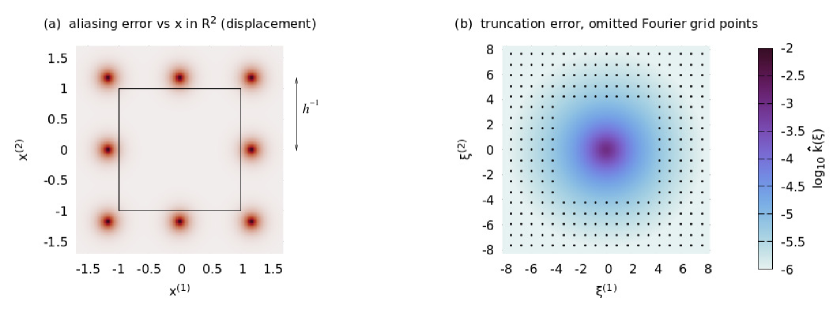
Figure 1: Illustration of two contributions to the discretization error in the pointwise approximation of the kernel $k(x)$, in $d=2$; see Section 3. Panel (a) shows the aliasing error term imaged as a function of the displacement argument $x$. The black square shows the domain $[-1,1]^{2}$. Panel (b) images $\hat{k}(\xi)$ (on a logarithmic color scale) in the Fourier plane, and shows as dots the punctured infinite lattice of excluded Fourier frequencies $hj$, where $j\in\mathbb{Z}^{2}$, $j\notin J_{m}$, and $J_{m}$ is the $(2m+1)$-by-$(2m+1)$ grid of quadrature nodes (not shown). The truncation error is bounded by the sum of $\hat{k}$ at all dots. The parameters (chosen merely for visual clarity) are $h=0.85$, $m=4$, for a Matérn kernel with $\nu=1/2$.

3.1 Squared-exponential kernel

Recall that for data points lying in $D=[0,1]^{d}$, the kernel $k(x)$ must be well approximated over $x\in[-1,1]^{d}$. The theorem below gives uniform bounds for the two contributions to the error. The result shows superexponential convergence both in $h$ (once $h<1$), and in $m$. In practice, for the typical case of $\ell\ll 1$, machine accuracy ($\approx 10^{-16}$) is reached once $h$ is less than 1 by a few times $\ell$, and $m$ is a couple times $1/\ell$.

In the proof below, the following elementary bounds on Gaussian sums are useful. For any $a>0$, we have by monotonicity,

$$\sum_{j=1}^{\infty}e^{-(aj)^{2}/2}\leq\int_{0}^{\infty}e^{-a^{2}t^{2}/2}dt=\frac{\sqrt{\pi}}{2a}$$ (20)

and hence

$$\sum_{j\in\mathbb{Z}}e^{-(aj)^{2}/2}=1+2\sum_{j=1}^{\infty}e^{-(aj)^{2}/2}\leq 1+\frac{\sqrt{\pi}}{a}.$$ (21)

We also need the Fourier transform of $G_{\ell}$ in (18), using the convention (12),

$$\hat{G}_{\ell}(\xi)=(\sqrt{2\pi}\ell)^{d}e^{-2|\pi\ell\xi|^{2}}.$$ (22)

Theorem 2 (Aliasing and truncation error for squared-exponential covariance kernel).

Suppose that $k(x)=G_{\ell}(x)$ as defined by (18), with length scale $\ell\leq 2/\sqrt{\pi}\approx 1.13$. Let $h<1$ be the frequency grid spacing. Then the aliasing error magnitude is bounded uniformly over $x\in[-1,1]^{d}$ by

$$\Biggl{|}\sum_{\begin{subarray}{c}n\in\mathbb{Z}^{d}\\ n\neq{\mathbf{0}}\end{subarray}}k\left(x+\frac{n}{h}\right)\Biggr{|}\;\leq\;2d\,3^{d}e^{-\frac{1}{2}\left(\frac{h^{-1}-1}{\ell}\right)^{2}}.$$ (23)

In addition, letting $m\in\mathbb{N}$ control the grid size ($2m+1$ in each dimension), the truncation error magnitude is bounded uniformly over $x\in\mathbb{R}^{d}$ by

$$\Biggl{|}h^{d}\sum_{\begin{subarray}{c}j\in\mathbb{Z}^{d}\\ j\notin J_{m}\end{subarray}}\hat{k}(jh)e^{2\pi ih\langle j,x\rangle}\Biggr{|}\;\leq\;2d\,4^{d}e^{-2(\pi\ell hm)^{2}}.$$ (24)

Proof of Theorem 2.

We first bound the aliasing error, by exploiting the fact that it is uniformly bounded over $[-1,1]$ by its value at $(1,0,\dots,0)$. Noting that $G_{\ell}$ is positive and isotropic, the left side of (23) is bounded by $2d$ equal sums over overlapping half-space lattices (pointing in each of the positive and negative coordinate directions),

$$\max_{x\in[-1,1]^{d}}\Biggl{|}\sum_{\begin{subarray}{c}n\in\mathbb{Z}^{d}\\ n\neq{\mathbf{0}}\end{subarray}}G_{\ell}\left(x-\frac{n}{h}\right)\Biggr{|}\;\leq\;2d\max_{x\in[-1,1]^{d}}\sum_{p=1}^{\infty}\sum_{q\in\mathbb{Z}^{d-1}}G_{\ell}\left(x-\frac{(p,q)}{h}\right)$$

$$\qquad=2d\,\biggl{(}\max_{s\in[-1,1]}\sum_{p=1}^{\infty}e^{-(s-p/h)^{2}/2\ell^{2}}\biggr{)}\biggl{(}\max_{t\in[-1,1]}\sum_{q\in\mathbb{Z}}e^{-(t-q/h)^{2}/2\ell^{2}}\biggr{)}^{d-1}$$ (25)

where in the second line we split off $s$ as the first coordinate of $x$, and used separability of the Gaussian. The sum over $q$ is bounded by its value for $t=0$, because, by the Poisson summation formula (17) and (22), this sum is equal for any $t\in\mathbb{R}$ to $h\sum_{j\in\mathbb{Z}}e^{2\pi ithj}\sqrt{2\pi}\ell e^{-2(\pi\ell hj)^{2}}$. Then setting $t=0$, this sum is bounded by using $a=1/h\ell$ in (21) to give

$$\max_{t\in[-1,1]}\sum_{q\in\mathbb{Z}}e^{-(t-q/h)^{2}/2\ell^{2}}\leq\sum_{q\in\mathbb{Z}}e^{-q^{2}/2h^{2}\ell^{2}}\leq 1+\sqrt{\pi}\ell h.$$ (26)

However, the first sum over $p$ in (25) is bounded by its value at $s=1$, which can be seen because $h<1$ thus each term is monotonically increasing in $s$. Then by writing $(1-p/h)^{2}=[(p-1)h^{-1}+(h^{-1}-1)]^{2}=(h^{-1}-1)^{2}+(p-1)^{2}h^{-2}+2(h^{-1}-1)h^{-1}(p-1)$ and noting that the last term is nonnegative,

$$\sum_{p=1}^{\infty}e^{-(1-p/h)^{2}/2\ell^{2}}\;\leq\;e^{-\mbox{\small$\frac{1}{2}$}\left(\frac{h^{-1}-1}{\ell}\right)^{2}}\sum_{p=1}^{\infty}e^{-(p-1)^{2}/2h^{2}\ell^{2}}\;\leq\;e^{-\mbox{\small$\frac{1}{2}$}\left(\frac{h^{-1}-1}{\ell}\right)^{2}}\left(1+\frac{\sqrt{\pi}\ell h}{2}\right),$$

where (20) was used with $a=1/h\ell$ in the last step. Inserting this and (26) into (25) and using $1+\sqrt{\pi}\ell h\leq 3$, implied by the hypotheses $h<1$ and $\ell\leq 2/\sqrt{\pi}$, finishes the proof of (23).

The proof of the truncation error bound is similar because $\hat{G}_{\ell}(\xi)$ in (18) is also Gaussian. Because $\hat{k}$ is always nonnegative, the left side of (24) is bounded by its value at $x={\mathbf{0}}$. As with the aliasing error, we may now bound the sum over the punctured lattice by that over $2d$ half-space lattices,

$$h^{d}\sum_{\begin{subarray}{c}j\in\mathbb{Z}^{d}\\ j\notin J_{m}\end{subarray}}\hat{k}(jh)\;=\;(\sqrt{2\pi}\ell h)^{d}\sum_{\begin{subarray}{c}j\in\mathbb{Z}^{d}\\ j\notin J_{m}\end{subarray}}e^{-\mbox{\small$\frac{1}{2}$}|2\pi\ell hj|^{2}}$$

$$\leq\;2d(\sqrt{2\pi}\ell h)^{d}\biggl{(}\sum_{p>m}e^{-\mbox{\small$\frac{1}{2}$}(2\pi\ell hp)^{2}}\biggr{)}\biggl{(}\sum_{q\in\mathbb{Z}}e^{-\mbox{\small$\frac{1}{2}$}(2\pi\ell hq)^{2}}\biggr{)}^{d-1}$$ (27)

The $q$ sum is bounded by $1+1/(2\sqrt{\pi}\ell h)$, by choosing $a=2\pi\ell h$ in (21). The $p$ sum is bounded by writing $p=m+j$, and dropping the nonnegative last term in $p^{2}=(m+j)^{2}=m^{2}+j^{2}+2mj$, then using (20), so

$$\sum_{p>m}e^{-\mbox{\small$\frac{1}{2}$}(2\pi\ell hp)^{2}}\;\leq\;e^{-2(\pi\ell hm)^{2}}\sum_{j=1}^{\infty}e^{-\mbox{\small$\frac{1}{2}$}(2\pi\ell hj)^{2}}\;\leq\;e^{-2(\pi\ell hm)^{2}}\left(1+\frac{1}{4\sqrt{\pi}\ell h}\right).$$

Replacing $4$ by $2$ in the above, then inserting these two bounds into (27) gives

$$h^{d}\sum_{\begin{subarray}{c}j\in\mathbb{Z}^{d}\\ j\notin J_{m}\end{subarray}}\hat{k}(jh)\;\leq\;2d\biggl{(}\sqrt{2\pi}\ell h+\frac{1}{\sqrt{2}}\biggr{)}^{d}e^{-2(\pi\ell hm)^{2}}.$$

The hypotheses $h<1$ and $\ell\leq 2/\sqrt{\pi}$ guarantee that the factor taken to the $d$th power is no more than $2\sqrt{2}+1/\sqrt{2}<4$, proving (24). ∎

The above leads to the following simple rule to set $h$ and $m$ to guarantee a user-defined absolute kernel approximation error, in exact arithmetic.

Corollary 3 (Discretization parameters $(h,m)$ to guarantee uniform SE kernel accuracy $\varepsilon$).

Let $k=G_{\ell}$ be the SE kernel, and let $\ell\leq 2/\sqrt{\pi}$ as above. Let $\varepsilon>0$. Set $h\leq\big{(}1+\ell\sqrt{2\log(4d\,3^{d}/\varepsilon)}\big{)}^{-1}$ then the aliasing error is no more than $\varepsilon/2$. In addition, set $m\geq\sqrt{\mbox{\small$\frac{1}{2}$}\log(4^{d+1}d/\varepsilon)}/\pi\ell h$, then the truncation error is no more than $\varepsilon/2$, so that $|\tilde{k}(x)-k(x)|\leq\varepsilon$ uniformly over $x\in[-1,1]^{d}$.

3.2 Matérn kernel

In this section we provide proofs for the aliasing error and truncation error estimates for the Matérn kernel given by (19). Its Fourier transform is

$$\hat{C}_{\nu,\ell}(\xi)=\hat{c}_{d,\nu}\left(\frac{\ell}{\sqrt{2\nu}}\right)^{d}\left(2\nu+|2\pi\ell\xi|^{2}\right)^{-\nu-d/2},$$ (28)

where $|\cdot|$, as before, denotes Euclidean norm, and where the prefactor $\hat{c}_{d,\nu}$ is

$$\hat{c}_{d,\nu}=\frac{2^{d}\pi^{d/2}(2\nu)^{\nu}\Gamma(\nu+d/2)}{\Gamma(\nu)}.$$ (29)

In order to prove the estimate for the aliasing error, we state some decay properties of the modified Bessel function $K_{\nu}(z)$ (using [21, 10.29 and 10.37] [15, §8.486]). For $z>0$, and fixed $\nu$, $K_{\nu}(z)$ is monotonically decreasing and positive. For fixed $z$, the modified Bessel functions are monotonically increasing in $\nu$, i.e. $K_{\nu}(z)\leq K_{\mu}(z)$ for $\mu\geq\nu$. Moreover,

$$\frac{d}{dz}(z^{\nu}K_{\nu}(z))=-z^{\nu}K_{\nu-1}(z)=-z^{\nu}\left(K_{\nu+1}(z)-\frac{2\nu}{z}K_{\nu}(z)\right).$$ (30)

Note that the positivity of $K_{\nu-1}(z)$ implies that $z^{\nu}K_{\nu}(z)$ is also a monotonically decreasing function of $z$. The monotonicity properties and the positivity of $K_{\nu}$ also imply that

$$\frac{1}{z^{\nu}K_{\nu}(z)}\frac{d}{dz}(z^{\nu}K_{\nu}(z))\;\leq\;-\frac{1}{2}\,,\qquad\forall z\geq 4\nu,$$ (31)

related to a special case in [2, Lem. 3]. Integrating the equation in $z$, we get the exponential upper bound

$$f_{\nu}(z):=z^{\nu}K_{\nu}(z)\;\leq\;f_{\nu}(4\nu)e^{2\nu}e^{-z/2}\,,\qquad z\geq 4\nu.$$ (32)

Noting that the Matérn kernel is proportional to $f_{\nu}(\sqrt{2\nu}|x|/\ell)$, this places a useful exponential decay bound on the kernel beyond a few $\ell$ away from its origin. Note that our bound is on $f_{\nu}(z)$ rather than $K_{\nu}(z)$ as in [2, Lem. 2], at the cost of a lower bound on $z$ and halving the exponential rate.

In order to prove the estimate for the truncation error in the following theorem, we first need the following lemma bounding power-law half-space lattice sums.

Lemma 4.

Let $\nu>0$, let $d\geq 1$, and let $m\geq 1$. Then

$$I(d,\nu,m):=\sum_{n>m}\sum_{q\in\mathbb{Z}^{d-1}}\left(n^{2}+|q|^{2}\right)^{-\nu-d/2}\leq\frac{\beta(d,\nu)}{m^{2\nu}}$$ (33)

where for fixed $\nu$ the prefactor $\beta$ obeys the following recursion relation in dimension $d$,

$$\beta(d,\nu)=\left\{\begin{array}[]{ll}\frac{1}{2\nu},&d=1\\ \left(4+\frac{2}{2\nu+d-1}\right)\beta(d-1,\nu),&d>1.\end{array}\right.$$ (34)

In particular, for any $\nu\geq 1/2$ we have

$$\beta(d,\nu)\leq\frac{5^{d-1}}{2\nu},\qquad d=1,2,\dots$$ (35)

Proof.

We observe for the case $d=1$ (upper case in (34)),

$$\sum_{n>m}n^{-2\nu-1}\leq\int_{m}^{\infty}y^{-2\nu-1}dy=\frac{m^{-2\nu}}{2\nu}$$ (36)

where monotonic decrease of the function was used to bound the sum by an integral. Now for $d>1$,

$$\sum_{n>m}\sum_{q\in\mathbb{Z}^{d-1}}\left(n^{2}+|q|^{2}\right)^{-\nu-d/2}=\sum_{n>m}\sum_{w\in\mathbb{Z}^{d-2}}\sum_{q\in\mathbb{Z}}\left(n^{2}+|w|^{2}+q^{2}\right)^{-\nu-d/2},$$

where in the case $d=2$ we abuse notation slightly: in that case the sum over $w$ is absent. We split the innermost sum into the central part $q\leq\lceil\sqrt{n^{2}+|w|^{2}}\rceil$, where $\lceil x\rceil$ denotes the smallest integer not less than $x$, plus the two-sided tail $q>\lceil\sqrt{n^{2}+|w|^{2}}\rceil$. The central part contains at most $2(\sqrt{n^{2}+|w|^{2}}+1)+1<4\sqrt{n^{2}+|w|^{2}}$ terms, where this upper bound follows since $n\geq 2$, and each such term is bounded by the constant $(n^{2}+|w|^{2})^{-\nu-d/2}$. The two-sided tail is bounded by $2\sum_{q>\lceil\sqrt{n^{2}+|w|^{2}}\rceil}(q^{2})^{-\nu-d/2}\leq 2\int_{\sqrt{n^{2}+|w|^{2}}}^{\infty}y^{-2\nu-d}dy=(2\nu+d-1)^{-1}(n^{2}+|w|^{2})^{-\nu-(d-1)/2}$. Combining both of these estimates, we get

$$I(d,\nu,m) \leq \left(4+\frac{2}{2\nu+d-1}\right)\sum_{n>m}\sum_{w\in Z^{d-2}}\left(n^{2}+|w|^{2}\right)^{-\nu-(d-1)/2}$$

$$= \left(4+\frac{2}{2\nu+d-1}\right)I(d-1,\nu,m).$$

Recursing down in $d$, we get (34), from which (35) follows immediately. ∎

We now present the main result: uniform bounds on the two contributions to the error for the Matérn kernel. The following shows exponential convergence with respect to $h$ for the aliasing error, but only order-$2\nu$ algebraic convergence with respect to $m$ for the truncation error. The latter is due to the algebraic tail of $\hat{C}_{\nu,\ell}(\xi)$.

Theorem 5 (Aliasing and truncation error for the Matérn covariance kernel).

Suppose $k(x)=C_{\nu,\ell}(x)$ as in (19), with smoothness $\nu\geq 1/2$ and length scale $\ell\leq(\log 2)^{-1}\sqrt{\nu/2d}$. Let $h\leq(1+\sqrt{8\nu}\ell)^{-1}$ be the frequency grid spacing. Then the aliasing error magnitude is bounded uniformly over $x\in[-1,1]^{d}$ by

$$\Biggl{|}\sum_{\begin{subarray}{c}n\in\mathbb{Z}^{d}\\ n\neq{\mathbf{0}}\end{subarray}}k\left(x+\frac{n}{h}\right)\Biggr{|}\;\leq\;4d\,3^{d-1}\cdot\frac{2^{1-\nu}}{\Gamma(\nu)}(4\nu)^{\nu}e^{2\nu}K_{\nu}(4\nu)\cdot e^{-\sqrt{\frac{\nu}{2d}}\frac{h^{-1}-1}{\ell}}.$$ (37)

In addition, letting $m\in\mathbb{N}$ control the grid size ($2m+1$ in each dimension), the truncation error magnitude is bounded uniformly over $x\in\mathbb{R}^{d}$ by

$$\Biggl{|}h^{d}\sum_{\begin{subarray}{c}j\in\mathbb{Z}^{d}\\ j\notin J_{m}\end{subarray}}\hat{k}(jh)e^{2\pi ih\langle j,x\rangle}\Biggr{|}\;\leq\;\frac{\nu^{\nu-1}d\,5^{d-1}}{2^{\nu}\pi^{d/2+2\nu}}\frac{\Gamma(\nu+1/2)}{\Gamma(\nu)}\frac{1}{(h\ell m)^{2\nu}}.$$ (38)

Proof of aliasing bound (37).

As with the squared-exponential case, we note that the sum over $n\in Z^{d}\setminus\{{\mathbf{0}}\}$ is bounded by $2d$ half-spaces of the form $p\geq 1$, $q\in\mathbb{Z}^{d-1}$, with $n=(p,q)$. Owing to the radial symmetry of the kernel, all of those half spaces can be bounded using the same estimate. Since $C_{\nu,\ell}(x)$ is positive we may remove absolute value signs. Substituting (19), and splitting $x=(s,t)$ where $s$ is the first coordinate and $t\in\mathbb{R}^{d-1}$,

$$\max_{x\in[-1,1]^{d}}\Biggl{|}\sum_{\begin{subarray}{c}n\in\mathbb{Z}^{d}\\ n\neq{\mathbf{0}}\end{subarray}}C_{\nu,\ell}\left(x-\frac{n}{h}\right)\Biggr{|}\;\leq\;2d\max_{x\in[-1,1]^{d}}\sum_{p=1}^{\infty}\sum_{q\in\mathbb{Z}^{d-1}}C_{\nu,\ell}\left(x-\frac{(p,q)}{h}\right)$$

$$\quad=\;2d\frac{2^{1-\nu}}{\Gamma(\nu)}\cdot\max_{s\in[-1,1],\,t\in[-1,1]^{d-1}}\sum_{p=1}^{\infty}\sum_{q\in\mathbb{Z}^{d-1}}f_{\nu}\biggl{(}\frac{\sqrt{2\nu}}{\ell}\sqrt{(p/h-s)^{2}+|q/h-t|^{2}}\biggr{)}$$

$$\quad\leq\;2d\frac{2^{1-\nu}}{\Gamma(\nu)}f_{\nu}(4\nu)e^{2\nu}\cdot\!\!\!\max_{s\in[-1,1],\,t\in[-1,1]^{d-1}}\sum_{p=1}^{\infty}\sum_{q\in\mathbb{Z}^{d-1}}\exp\biggl{(}-\frac{\sqrt{\nu}}{\sqrt{2}\ell}\sqrt{(p/h-s)^{2}+|q/h-t|^{2}}\biggr{)}$$

where in the last step we applied the exponential decay bound (32) to each term in the sum. This is valid since no distance from the kernel origin (square root in the above) is less than $(h^{-1}-1)/\ell$, which is at least $\sqrt{8\nu}$ by the hypothesis on $h$. We now lower-bound the square-root via $\|y\|_{2}\geq\|y\|_{1}/\sqrt{d}$ for any $y\in\mathbb{R}^{d}$, which follows from Cauchy–Schwarz. The product now separates along dimensions, so the above is bounded by

$$2d\frac{2^{1-\nu}}{\Gamma(\nu)}f_{\nu}(4\nu)e^{2\nu}\cdot\biggl{(}\max_{s\in[-1,1]}\sum_{p=1}^{\infty}e^{-\sqrt{\frac{\nu}{2d}}\frac{1}{\ell}(p/h-s)}\biggr{)}\biggl{(}\max_{t\in[-1,1]}\sum_{q\in\mathbb{Z}}e^{-\sqrt{\frac{\nu}{2d}}\frac{1}{\ell}|q/h-t|}\biggr{)}^{d-1}\leavevmode\nobreak\ .$$ (39)

In the first sum each term is maximized at $s=1$, so writing $p^{\prime}=p-1$ we bound that sum geometrically by

$$e^{-\sqrt{\frac{\nu}{2d}}\frac{h^{-1}-1}{\ell}}\sum_{p^{\prime}=0}^{\infty}e^{-\sqrt{\frac{\nu}{2d}}\frac{p^{\prime}}{\ell h}}\;\leq\;\frac{e^{-\sqrt{\frac{\nu}{2d}}\frac{h^{-1}-1}{\ell}}}{1-e^{-\sqrt{\frac{\nu}{2d}}\frac{1}{\ell h}}}\;\leq\;2e^{-\sqrt{\frac{\nu}{2d}}\frac{h^{-1}-1}{\ell}}$$

where in the last step we used the hypothesis $\ell\leq(\log 2)^{-1}\sqrt{\nu/2d}$ and $h<1$ to upper-bound the geometric factor by $1/2$.

The second sum over $q$ in (39) is bounded by its value for $t=0$, because by the Poisson summation formula (17) it is equal for any $t\in\mathbb{R}$ to $h\sum_{j\in\mathbb{Z}}e^{2\pi ithj}\frac{2\beta}{\beta^{2}+(2\pi hj)^{2}}$ where $\beta=\sqrt{\nu/2}\ell^{-1}$. This relies on the Fourier transform of $e^{-\beta|t|}$ being the everywhere-positive function $\frac{2\beta}{\beta^{2}+(2\pi\xi)^{2}}$. Thus we set $t=0$ in this second sum, write it as two geometric series with geometric factor again at most $1/2$, which upper bounds the sum by $3$. Substituting the above two sum bounds into (39) proves (37). ∎

Proof of truncation bound (38).

Now we use Lemma 4 of half-space lattice sums to complete the proof of Theorem 5. Noting that $\hat{k}=\hat{C}_{\nu,\ell}$ from (28) is always positive, we may drop the phases to get a uniform upper bound,

$$\Biggl{|}h^{d}\!\sum_{\begin{subarray}{c}j\in\mathbb{Z}^{d}\\ j\not\in J_{m}\end{subarray}}\hat{C}_{\nu,\ell}(jh)e^{2\pi ih\langle j,x\rangle}\Biggr{|} \leq h^{d}\!\!\sum_{j\in\mathbb{Z}^{d}\backslash J_{m}}\hat{C}_{\nu}(jh,\ell)=\hat{c}_{d,\nu}(h\ell)^{d}\!\!\sum_{j\in\mathbb{Z}^{d}\backslash J_{m}}(2\nu+|2\pi\ell hj|^{2})^{-\nu-d/2}$$

$$\leq \frac{\hat{c}_{d,\nu}}{(2\pi)^{2\nu+d}}(h\ell)^{-2\nu}\sum_{j\in\mathbb{Z}^{d}\backslash J_{m}}|j|^{-2\nu-d}$$

$$\leq \frac{\hat{c}_{d,\nu}}{(2\pi)^{2\nu+d}}(h\ell)^{-2\nu}\cdot 2d\sum_{n>m}\sum_{q\in\mathbb{Z}^{d-1}}(n^{2}+|q|^{2})^{-\nu-d/2}$$

$$= \frac{\hat{c}_{d,\nu}}{(2\pi)^{2\nu+d}}\frac{2d\,I(d,\nu,m)}{(h\ell)^{2\nu}}\;\leq\;\frac{\hat{c}_{d,\nu}}{(2\pi)^{2\nu+d}}\frac{5^{d-1}}{2\nu}\frac{2d}{(h\ell m)^{2\nu}}.$$

Here the third inequality follows from noting (similarly to the previous proofs) that the sum over $j\in\mathbb{Z}^{d}\backslash J_{m}$ is bounded by $2d$ lattice half-spaces of the form $n>m$, $q\in\mathbb{Z}^{d-1}$. The last inequality follows from Lemma 4. Substituting (29) gives (38); the theorem is proved. ∎

As with the SE kernel, this theorem leads to a simple rule to set $h$ and $m$ to guarantee a user-defined absolute kernel approximation error. In the following we restrict to small dimension, and use that the $\nu$-dependent middle factor in (37) never exceeds $3/8$, and $(2\Gamma(\nu+d/2)/\nu\Gamma(\nu))^{1/2\nu}/\sqrt{2}<1.6$ for $\nu\geq 1/2$, $d\leq 3$.

Corollary 6 (Discretization parameters $(h,m)$ to guarantee uniform Matérn kernel accuracy $\varepsilon$).

Let the dimension $d$ be 1, 2, or 3. Let $k=C_{\nu,\ell}$ be the Matérn kernel with $\nu\geq 1/2$ and $\ell\leq(\log 2)^{-1}\sqrt{\nu/2d}$ as above. Let $\varepsilon>0$. Set $h\leq\big{(}1+\ell\sqrt{2d/\nu}\log(d\,3^{d}/\varepsilon)\big{)}^{-1}$, then the aliasing error is no more than $\varepsilon/2$. In addition, set $m\geq(d\,5^{d-1}/\pi^{d/2}\varepsilon)^{1/2\nu}\cdot(1.6)\sqrt{\nu}/\pi h\ell$, then the truncation error is no more than $\varepsilon/2$, so that the error obeys $|\tilde{k}(x)-k(x)|\leq\varepsilon$ uniformly over $x\in[-1,1]^{d}$.

Note that holding $\nu$, $\ell$ and $h$ fixed, $m={\mathcal{O}}(1/\varepsilon^{1/2\nu})$ as expected from truncating the Matérn Fourier transform with algebraic decay $1/|\xi|^{2\nu+d}$ (see (28)). Instead holding tolerance $\varepsilon$ fixed, $m={\mathcal{O}}(1/\ell)$ as $\ell\to 0$, as expected from the growing number of oscillations in the interpolant across the linear extent of the domain. The above corollary should be compared with [2, (1.11)], where $\gamma$ plays the role of $h^{-1}$. In order to minimize the $m$ used in practice, instead of the above rigorous parameters choices we recommend more forgiving heuristics that we state in the next section.

Remark 7.

Both Theorems 2 and 5 have the very mild restrictions that $\ell$ be smaller than some ${\mathcal{O}}(1)$ constant. These are in practice irrelevant because the domain $D$ is also of size 1 in each dimension, and in all applications known to us $\ell$ is set substantially smaller than the domain size (otherwise the prior covariance is so long-range that the regression output would be nearly constant over the domain).

Remark 8.

Theorems 2 and 5 have all prefactors explicit. It may be possible to improve the prefactors of the form $dc^{d}$ where $2\leq c\leq 5$, since these are due to overcounting where half-spaces overlap and bounds on sums over $\mathbb{Z}^{d-1}$ that could be improved. The $1/\sqrt{d}$ factor in the exponential in (37) might also be removable by using partial Poisson summation.

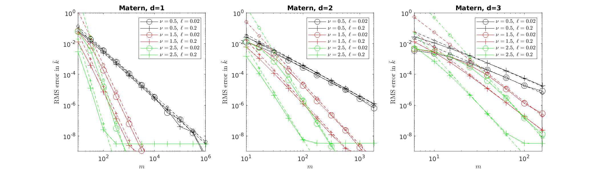
Figure 2: Estimated root mean square approximation error for the Matérn kernel in dimensions $d=1,2,3$ with various parameters, compared to the heuristic $\tilde{\varepsilon}$ of (40) with prefactor as in Remark 10. The proposed equispaced Fourier basis is used. RMS error is found via high-order accurate quadrature for the double integral (41) rewritten as $\int_{[-1,1]^{d}}v(z)|\tilde{k}(z)-k(z)|^{2}dz$ where $v$ is the autocorrelation of $\rho$, for the choice $\rho\equiv 1$ in $D$. For each choice of $\nu$ and $\ell$, the solid line shows the error, while the dotted line shows the heuristic. $h$ was chosen via (44) to achieve aliasing error $\varepsilon=10^{-8}$.

4 Matérn covariance matrix approximation error

For sufficiently non-smooth Matérn kernels, such as $\nu\leq 3/2$, the uniform truncation error bound (38) dominates and gives slow algebraic convergence ${\mathcal{O}}(1/m^{2\nu})$, due to slow decay in Fourier space. Yet we have observed that in practice this bound is overly pessimistic when it comes to the more relevant root mean square error of covariance matrix elements, leading to wasted computational effort. We instead propose (and use [16, Sec. 4.2]) the following heuristic with faster convergence ${\mathcal{O}}(1/m^{2\nu+d/2})$.

Conjecture 9 (equispaced Fourier Matérn covariance matrix error).

Let the points $x_{1},\dots,x_{N}$ be iid drawn from some bounded probability density function $\rho$ with support in $D=[0,1]^{d}$. Let the Matérn kernel with parameters $\nu$ and $\ell$ be approximated by equispaced Fourier modes as in Theorem 5, with $h$ and $m$ chosen so that the aliasing error is negligible compared to the truncation error. Then with high probability as $N\to\infty$,

$$\|\tilde{K}-K\|_{F}\leq N\tilde{\varepsilon},\qquad\mbox{the root mean square error being}\quad\tilde{\varepsilon}=\frac{\tilde{c}_{d,\nu,\rho}}{\ell^{2\nu}(hm)^{2\nu+d/2}},$$ (40)

for some constant $\tilde{c}_{d,\nu,\rho}$ independent of $N$, $\ell$, $h$, and $m$.

Justification of Conjecture 9.

Regardless of the kernel or its approximation method, the expectation (over data point realizations) of the squared Frobenius norm is

$$\mathbb{E}\|\tilde{K}-K\|^{2}_{F}=\mathbb{E}\sum_{n,n^{\prime}=1}^{N}|\tilde{K}_{n,n^{\prime}}-K_{n,n^{\prime}}|^{2}=N^{2}\int_{D}\int_{D}|\tilde{k}(x-x^{\prime})-k(x-x^{\prime})|^{2}\rho(x)\rho(x^{\prime})dxdx^{\prime}.$$ (41)

Now substituting the dominant truncation part of the pointwise error formula (16), and changing variable to $z=x-x^{\prime}$ which ranges over the set $D-D=[-1,1]^{d}$, with $dxdx^{\prime}=dzdx^{\prime}$, we get

$$\mathbb{E}\|\tilde{K}-K\|^{2}_{F} \approx N^{2}h^{2d}\sum_{j,j^{\prime}\notin J_{m}}\hat{k}(hj)\hat{k}(hj^{\prime})\int_{[-1,1]^{d}}\!\!\!e^{2\pi i\langle h(j-j^{\prime}),z\rangle}\left(\int_{D}\rho(z+x^{\prime})\rho(x^{\prime})dx^{\prime}\right)dz$$ (42)

$$= N^{2}h^{2d}\sum_{j,j^{\prime}\notin J_{m}}\hat{k}(hj)\hat{k}(hj^{\prime})\,|\hat{\rho}(h(j-j^{\prime}))|^{2},$$

where the last step used the Wiener–Khintchine theorem for the Fourier transform of the autocorrelation of $\rho$. In a mean-square sense with respect to angle we expect Fourier decay $\hat{\rho}(\xi)={\mathcal{O}}(1/|\xi|^{(1+d)/2})$, even if $\rho$ has discontinuities (e.g., see [5] for the case of $\rho\equiv 1$ in $D$, and we may approximate $\rho$ by a linear combination of such characteristic functions of convex sets). Since $|\hat{\rho}(hj)|^{2}$ is then summable over $j\in\mathbb{Z}^{d}$, and the small $j,j^{\prime}$ terms dominate (as in the Gibbs phenomenon), we expect that there is a constant $c_{\rho}>0$ independent of $m$ such that

$$h^{2d}\sum_{j,j^{\prime}\notin J_{m}}\hat{k}(hj)\hat{k}(hj^{\prime})\,|\hat{\rho}(h(j-j^{\prime}))|^{2}\;\leq\;c_{\rho}h^{2d}\sum_{j\notin J_{m}}|\hat{k}(hj)|^{2}\;=\;{\mathcal{O}}\bigl{(}1/\ell^{4\nu}(hm)^{4\nu+d}\bigr{)},$$

where in the last step we used the decay of $\hat{k}(hj)$ from (28), with the sum losing one power of $d$ as in the proof of Theorem 5. Finally, by the central limit theorem we expect, with high probability as $N\to\infty$, that $\|\tilde{K}-K\|_{F}^{2}$ tends to its expectation, justifying (40).

A rigorous proof of the conjecture, even for the easiest case $\rho\in C_{0}^{\infty}(D)$, is an open problem. We note that related work exists in the variational GP setting [6]. Although the iid assumption on data points cannot be justified in many settings (e.g., satellite data), we find the conjecture very useful to set numerical parameters even in such cases. We summarize the resulting empirically good parameter choices in the following remark.

Remark 10 (Discretization parameters $(h,m)$ to achieve empirical root-mean-square Matérn kernel accuracy $\varepsilon$).

By numerical study of the constant-density case $\rho\equiv 1$ in the domain $D=[0,1]^{d}$, we fit the prefactor $\tilde{c}_{d,\nu,1}\approx 0.15/\pi^{\nu+d/2}$ in (40). Figure 2 shows that this truncation prediction matches to within a fraction of a decimal digit the estimated root mean square error $\tilde{\varepsilon}$. Inverting this gives our proposed numerical grid size choice

$$m\;\approx\;\frac{1}{h}\biggl{(}\pi^{\nu+d/2}\ell^{2\nu}\frac{\varepsilon}{0.15}\biggr{)}^{-1/(2\nu+d/2)}$$ (43)

to achieve root-mean square truncation error around the given $\varepsilon$. The scaling $m={\mathcal{O}}(1/\varepsilon^{1/(2\nu+d/2)})$ is more forgiving than the rigorous ${\mathcal{O}}(1/\varepsilon^{1/2\nu})$ of Corollary 6, resulting in a smaller grid. For instance, for $\nu=1/2$ this lowers $M={\mathcal{O}}(m^{d})$, the total number of modes to achieve a Frobenius norm of $N\varepsilon$, from $M={\mathcal{O}}(1/\varepsilon^{d})$ to $M={\mathcal{O}}(1/\varepsilon^{2d/(2+d)})$, a significant reduction in numerical effort when $d$ is “large” (eg $3$).

We also find that a practical choice of $h$ to bound aliasing error by a given $\varepsilon$ is

$$h\;\approx\;\bigl{(}1+0.85(\ell/\sqrt{\nu})\log 1/\varepsilon\bigr{)}^{-1},\qquad 1/2\leq\nu\leq 5/2.$$ (44)

This is also verified (for a single $\varepsilon$ choice) by the saturation of error at a minimum around $10^{-8}$ in Figure 2. This $h$ is larger than that in Corollary 6, allowing $M$, hence the computation time, to be further reduced.

We provide extensive numerical experiments using these parameter choices in [16], but do not dwell on them further, since the meat of the present work is the rigorous analysis.

Figure 3: Condition numbers of the weight-space system matrix $A_{\mbox{\tiny\rm WS}}:=\Phi^{*}\Phi+\sigma^{2}I$, the approximate function-space system matrix $A_{\mbox{\tiny\rm FS}}:=\Phi\Phi^{*}+\sigma^{2}I$, and the exact function-space matrix $K+\sigma^{2}I$, as a function of the number of data points $N$, for $d=1$. The $\kappa_{\mbox{\tiny\rm FS}}$ curve (black) lies completely under the exact $\kappa$ (green) curve. The data points are uniform random on $[0,1]$, for a squared-exponential kernel with $\ell=0.1$, and noise $\sigma=0.3$.

(a) $\log_{10}\kappa_{\mbox{\tiny\rm WS}}$

(b) $\log_{10}$ of bound (47)

(c) Ratio of $\kappa_{\mbox{\tiny\rm WS}}$ to bound (47)

Figure 4: Panel (a) shows the condition number of the weight space system matrix $\Phi^{*}\Phi+\sigma^{2}I$ for various $N$ and $\sigma^{2}$. (b) shows its upper bound (in the limit $\varepsilon\to 0$). (c) plots the ratio between the two, which is nearly constant at around 0.54. Other parameters are as in Figure 3.

5 Conditioning of function-space and weight-space systems

In [16] it was observed that the iteration count for conjugate gradient solution with EFGP often grew with the number of data points, and alarmingly so at smaller tolerance $\varepsilon$. To grapple with this, in this final section we present some preliminary analysis that applies to any approximate-factorization GP regression method, connect the weight-space and function-space linear system condition numbers, and perform a numerical study in the EFGP case. We do not address preconditioning, but note that it has been beneficial in the GP context [26, 12, 28].

Recall that “exact” GP regression requires a solution to the function space linear system

$$(K+\sigma^{2}I)\bm{\alpha}={\mathbf{y}},$$ (45)

and that GP regression using an approximate factorization of the kernel, in function or weight space, requires solutions to linear systems with system matrices

$$A_{{\mbox{\tiny\rm FS}}}=\Phi\Phi^{*}+\sigma^{2}I,\qquad A_{{\mbox{\tiny\rm WS}}}=\Phi^{*}\Phi+\sigma^{2}I,$$ (46)

respectively, where $\Phi$ is some $N$-by-$M$ design matrix with $\Phi\Phi^{*}=\tilde{K}\approx K$. In the special case of EFGP we described the matrix $\Phi$ in Section 2.2. From now we assume that the data size $N$ is large enough so that $N>M$.

We start with a simple bound for the exact GP regression function space system.

Proposition 11 (Exact function space condition number bound).

Let $k:\mathbb{R}^{d}\to\mathbb{R}$ be a translationally invariant positive semidefinite covariance kernel with $k({\mathbf{0}})=1$. Let $x_{1},\dots,x_{N}\in\mathbb{R}^{d}$, and $K$ be the $N\times N$ covariance matrix with $ij$th element $k(x_{i}-x_{j})$. Then the condition number of the GP function space system matrix obeys

$$\kappa(K+\sigma^{2}I)\;\leq\;\frac{N}{\sigma^{2}}+1.$$ (47)

Proof.

Since $k$ is a positive semidefinite kernel, meaning $\hat{k}$ is nonnegative [23, §4.1], then $|k(x)|=|\int_{\mathbb{R}^{d}}e^{2\pi i\langle x,\xi\rangle}\hat{k}(\xi)d\xi|\leq\int_{\mathbb{R}^{d}}\hat{k}(\xi)d\xi=k({\mathbf{0}})=1$. Thus all entries of $K$ are bounded in magnitude by $1$, so $\|K\|_{F}\leq N$. Since the spectral norm is bounded by the Frobenius norm, the largest eigenvalue of $K$ is no more than $N$ (or see [30, p. 207]), and so the hence spectral norm of $K+\sigma^{2}I$ is no more than $N+\sigma^{2}$. Since $K$ is positive definite, its eigenvalues are nonnegative, so that no eigenvalue of $K+\sigma^{2}I$ is less than $\sigma^{2}$. The proof is completed since $\kappa(K+\sigma^{2}I)$ is the ratio of maximum to minimum eigenvalues, because $K$ is symmetric. ∎

The upper bound is sharp, since $K$ may come arbitrarily close to the matrix with all entries $1$ when all data points approach the same point. The trivial lower bound $\kappa(K+\sigma^{2}I)\geq 1$ is also sharp since $K$ approaches $I$ when all data points move far from each other compared to the kernel width $\ell$. Only with assumptions on the distribution of data points (their typical separation compared to $\ell$) could stronger statements be made. For instance, for fixed $k$ and data domain, as $N\to\infty$ then $\kappa(K+\sigma^{2}I)$ grows no slower than $cN/\sigma^{2}$ for some $c>0$ (this follows from [26, p. 54]). Note that Proposition 11 could be generalized to the case $k({\mathbf{0}})\neq 1$ simply by replacing $\sigma^{2}$ by $\sigma^{2}/k({\mathbf{0}})$ in the right-hand side of (47).

Remark 12.

The bound (47) is large in practice: for instance in a typical big problem with $N=10^{7}$ and $\sigma=0.1$, the bound allows $\kappa$ to be $10^{9}$, meaning that using single precision there may be no correct digits in the solution $\bm{\alpha}$ to the function space GP linear system (5), and possibly catastrophic cancellation in evaluation of the posterior mean.

Two natural questions now arise: i) Is the GP regression problem itself as ill-conditioned as the above suggests? ii) Is the weight-space system matrix $A_{{\mbox{\tiny\rm WS}}}$ similarly conditioned to the (exact) function-space matrix $K+\sigma^{2}I$ ? We now show that the answers are respectively “no” and “typically yes.”

Proposition 13 (The GP regression problem at the data points is well-conditioned).

Given data points $x_{1},\dots,x_{N}\in\mathbb{R}^{d}$, a positive definite kernel, and $\sigma>0$, the absolute condition number of the map from the data vector ${\mathbf{y}}$ to the posterior mean $\bm{\mu}:=\{\mu(x_{n})\}_{n=1}^{N}$ is less than 1.

Proof.

Since the resulting $K$ is positive semidefinite [23, Ch. 4], it may be orthogonally diagonalized as $K=\sum_{n=1}^{N}\lambda_{n}{\mathbf{v}}_{n}{\mathbf{v}}_{n}^{\mathsf{T}}$ with $\lambda_{n}\geq 0$ and $\|{\mathbf{v}}_{n}\|=1$, so the solution is $\bm{\mu}=K\bm{\alpha}=K(K+\sigma^{2}I)^{-1}{\mathbf{y}}=\sum_{n}\lambda_{n}(\lambda_{n}+\sigma^{2})^{-1}{\mathbf{v}}_{n}{\mathbf{v}}_{n}^{\mathsf{T}}{\mathbf{y}}$. Thus the solution operator has spectral norm $\max_{n}\lambda_{n}/(\lambda_{n}+\sigma^{2})<1$. ∎

Thus this regression problem remains well conditioned, even as $N$ grows or $\sigma\to 0$, when (as shown above and below) the system matrix can become very ill-conditioned! One might worry that an algorithm that solves such an ill-conditioned system is unstable, for instance unnecessarily amplifying the kernel error $\varepsilon$. In exact arithmetic, (9) bounds such amplification by the (large) constant $N/\sigma^{2}$. In floating point arithmetic the situation may be more dire, due to catastrophic cancellation in evaluating $\bm{\mu}=\Phi\bm{\beta}$, if $\|\bm{\beta}\|$ is large.

For $\mu(x)$ at new targets, even less is known (at least to these authors): it is unknown whether the absolute condition number of the regression problem is even ${\mathcal{O}}(1)$, or whether the extremely large $N^{2}/\sigma^{4}$ amplification factor in the naive bound (10) could be reduced.

We now turn to question ii): how close are the condition numbers of the weight-space $A_{\mbox{\tiny\rm WS}}$, approximate function-space $A_{\mbox{\tiny\rm FS}}$, and exact function-space $K+\sigma^{2}I$ system matrices? We now show, as $\varepsilon\to 0$ (good kernel approximation), that neither of the two approximate linear systems can be worse conditioned than the exact one. To interpret the following, recall from (7) that a pointwise kernel error of $\varepsilon$ leads to the simple bound $\|\tilde{K}-K\|\leq N\varepsilon$.

Lemma 14 (Approximated linear system condition number bounds).

Let $\Phi\in\mathbb{C}^{N\times M}$ with $M<N$, such that $\tilde{K}=\Phi\Phi^{*}$ approximates $K$ to spectral norm error $\|\tilde{K}-K\|\leq N\varepsilon$. Then the approximated function-space condition number denoted by $\kappa_{{\mbox{\tiny\rm FS}}}=\kappa(A_{{\mbox{\tiny\rm FS}}})$, and the weight space condition number denoted by $\kappa_{{\mbox{\tiny\rm WS}}}=\kappa(A_{{\mbox{\tiny\rm WS}}})$, both have an upper bound

$$\kappa_{{\mbox{\tiny\rm FS}}},\kappa_{\mbox{\tiny\rm WS}}\;\leq\;\biggl{(}1+\frac{\varepsilon N}{\sigma^{2}}\biggr{)}\kappa(K+\sigma^{2}I)+\frac{\varepsilon N}{\sigma^{2}}.$$ (48)

Proof.

Our main tool is eigenvalue perturbation: for each eigenvalue of $K$ there is an eigenvalue of $\tilde{K}$ within a distance of $\varepsilon N$, which follows from the symmetric case of the Bauer–Fike theorem [14, Thm. 7.7.2] and $\|\tilde{K}-K\|\leq\varepsilon N$. Since $M<N$, $\tilde{K}$ has a zero eigenvalue, so the minimum eigenvalue of $K$ is $\lambda_{\text{min}}\in[0,\varepsilon N]$. Abbreviating $\kappa:=\kappa(K+\sigma^{2}I)=(\lambda_{\text{max}}+\sigma^{2})/(\lambda_{\text{min}}+\sigma^{2})$, then $\lambda_{\text{max}}\leq(\sigma^{2}+\varepsilon N)\kappa-\sigma^{2}$. Again by eigenvalue perturbation, the largest eigenvalue of $\tilde{K}$ is no more than $\lambda_{\text{max}}+\varepsilon N\leq(\sigma^{2}+\varepsilon N)\kappa-\sigma^{2}+\varepsilon N$, and the same is true for $\Phi^{*}\Phi$ since its nonzero eigenvalues match those of $\tilde{K}$. Thus $\|\Phi^{*}\Phi+\sigma^{2}I\|\leq(\sigma^{2}+\varepsilon N)\kappa+\varepsilon N$. Finally, since $\|(\Phi^{*}\Phi+\sigma^{2}I)^{-1}\|\leq\sigma^{-2}$, and $\|(\Phi\Phi^{*}+\sigma^{2}I)^{-1}\|=\sigma^{-2}$, the results then follow. ∎

We now report a test of empirical condition number growth vs $N$ and $\sigma^{-2}$, for random data in $d=1$. Figures 3 and 4 compare $\kappa(K+\sigma^{2}I)$, $\kappa_{{\mbox{\tiny\rm FS}}}$, $\kappa_{\mbox{\tiny\rm WS}}$, and also the theoretical upper bound $N/\sigma^{2}+1$ from (47). The upper bound applies to all three as $\varepsilon\to 0$. The plots show that the three condition numbers are extremely close to each other, and that the bound overestimates them by only a factor of roughly $2$, over a wide $(N,\sigma)$ parameter space. Here we used dense symmetric diagonalization for the “exact” calculations of $\kappa(K+\sigma^{2}I)$ and $\kappa_{\mbox{\tiny\rm FS}}$ for $N\leq 10^{4}$, and EFGP with $\varepsilon$ converged down to $10^{-16}$ (i.e., machine precision) for the other cases. By Corollary 3 this requires only a small $m<30$, for which dense diagonalization of $A_{\mbox{\tiny\rm WS}}$ is trivial.

Finally, the above has consequences for the convergence rate of conjugate gradient to solve either function-space or weight-space linear systems. For instance, if $\bm{\beta}$ is the exact solution to (15), and $\bm{\beta}_{k}$ its approximation at the $k$th CG iteration [14, §10.2],

$$\|\bm{\beta}_{k}-\bm{\beta}\|\;=\;{\mathcal{O}}\bigg{(}\bigg{(}\frac{\sqrt{\kappa_{\mbox{\tiny\rm WS}}}-1}{\sqrt{\kappa_{\mbox{\tiny\rm WS}}}+1}\bigg{)}^{k}\bigg{)}.$$ (49)

Since $\kappa_{\mbox{\tiny\rm WS}}\lesssim N/\sigma^{2}$ for small $\varepsilon$, this gives convergence no slower than $e^{-(2\sigma/\sqrt{N})k}$. Thus one requires at most ${\mathcal{O}}\bigl{(}\log(1/\varepsilon)\sqrt{N}/\sigma\bigr{)}$ iterations to reach a residual $\varepsilon$.

6 Conclusions and generalizations

In this paper, we provided a detailed error analysis for the equispaced Fourier Gaussian process (EFGP) kernel representation of [16]. The main results (Theorems 2 and 5) gave uniform kernel approximation error bounds for the popular squared-exponential and Matérn kernels, with all constants explicit, in general dimension. This led to Fourier quadrature grid parameters that guarantee a desired kernel error (Corollaries 3 and 6). Since this equispaced Fourier grid is maybe the simplest spectral kernel approximation, we expect these to find applications in other kernel methods.

For the Matérn kernel with small $\nu$, these uniform error bounds are in practice pessimistic when it comes to root mean square errors, because of the slow Fourier decay of the kernel. Thus we proposed a conjecture on the root mean square kernel error, and supported it by numerical tests. A proof, even for iid random data coming from a smooth density function, remains open.

Finally, we proved an upper bound on the condition number of the approximate function- and weight-space linear systems for arbitrary data distributions, showing how they approach the “exact” GP condition number as the kernel approximation error vanishes. We then showed experimentally that such condition numbers for a simple random data point distribution are about as ill-conditioned as possible, i.e., within a small factor of $N/\sigma^{2}$. Yet, Proposition 13 reminds one that the GP regression problem itself (at least for the mean at the data points themselves) is well conditioned. In short, an ill-conditioned algorithm appears to be necessary to solve a well-conditioned problem, raising the eyebrows of any numerical analyst. This motivates the future study of stability (coefficient norm growth and the resulting rounding loss) in GP settings, especially in an era of reduced (e.g. half-) precision arithmetic. It also suggests the continued study of preconditioners for GP regression problems.

Many other interesting analysis questions remain, such as Fourier kernel approximation bounds for other common kernels, the conditioning of the regression problem to new targets, and a rigorous lower bound on $\kappa_{\mbox{\tiny\rm WS}}$ (analogous to Lemma 14), which would demand knowledge of $K$’s smallest eigenvalue.

References

- [1] S. Ambikasaran, D. Foreman-Mackey, L. Greengard, D. W. Hogg, and M. O’Neil. Fast direct methods for Gaussian processes. IEEE Trans. Pattern Anal. Mach. Intell., 38(2):252–265, 2016.
- [2] M. Bachmayr, I. G. Graham, V. K. Nguyen, and R. Scheichl. Unified analysis of periodization-based sampling methods for Matérn covariances. SIAM J. Numer. Anal., 58(5):2953–2980, 2020.
- [3] A. P. Bartók, M. C. Payne, R. Kondor, and G. Csányi. Gaussian approximation potentials: The accuracy of quantum mechanics, without the electrons. Phys. Rev. Lett., 104:136403, Apr 2010.
- [4] S. Baugh and M. L. Stein. Computationally efficient spatial modeling using recursive skeletonization factorizations. Spatial Statistics, 27:18–30, 2018.
- [5] L. Brandolini, S. Hofmann, and A. Iosevich. Sharp rate of average decay of the Fourier transform of a bounded set. Geometric and Functional Analysis GAFA, 13(4):671, 2003.
- [6] D. Burt, C. E. Rasmussen, and M. Van Der Wilk. Rates of convergence for sparse variational Gaussian process regression. In K. Chaudhuri and R. Salakhutdinov, editors, Proceedings of the 36th International Conference on Machine Learning, volume 97 of Proceedings of Machine Learning Research, pages 862–871. PMLR, 09–15 Jun 2019.
- [7] J. Chen and M. Stein. Linear-cost covariance functions for Gaussian random fields. Journal of the American Statistical Association, pages 1–18, 2021.
- [8] N. Cressie. Mission CO2ntrol: A statistical scientist’s role in remote sensing of atmospheric carbon dioxide. Journal of the American Statistical Association, 113(521):152–168, 2018.
- [9] G. Dahlquist and A. Bjork. Numerical Methods. Dover, Mineola, NY, 1974.
- [10] A. Dutt and V. Rokhlin. Fast Fourier transforms for nonequispaced data. SIAM Journal on Scientific Computing, 14(6):1368–1393, 1993.
- [11] D. Foreman-Mackey, E. Agol, S. Ambikasaran, and R. Angus. Fast and scalable Gaussian process modeling with applications to astronomical time series. The Astronomical Journal, 154(6), 2017.
- [12] J. Gardner, G. Pleiss, K. Q. Weinberger, D. Bindel, and A. G. Wilson. GPyTorch: Blackbox matrix-matrix Gaussian process inference with GPU acceleration. In S. Bengio, H. Wallach, H. Larochelle, K. Grauman, N. Cesa-Bianchi, and R. Garnett, editors, Advances in Neural Information Processing Systems, volume 31. Curran Associates, Inc., 2018.
- [13] A. Gelman, J. B. Carlin, H. S. Stern, D. B. Dunson, A. Vehtari, and D. B. Rubin. Bayesian Data Analysis. Chapman and Hall/CRC, New York, NY, 3rd edition, 2013.
- [14] G. H. Golub and C. F. van Loan. Matrix computations. Johns Hopkins Studies in the Mathematical Sciences. Johns Hopkins University Press, Baltimore, MD, third edition, 1996.
- [15] I. S. Gradshteyn and I. M. Ryzhik. Table of integrals, series, and products. Academic press, 8th edition, 2014.
- [16] P. Greengard, M. Rachh, and A. Barnett. Equispaced Fourier representations for efficient Gaussian process regression from a billion data points, 2023. submitted, SIAM ASA J. Uncert. Quant.
- [17] M. J. Heaton, A. Datta, A. O. Finley, R. Furrer, J. Guinness, R. Guhaniyogi, F. Gerber, R. B. Gramacy, D. Hammerling, M. Katzfuss, F. Lindgren, D. W. Nychka, F. Sun, and A. Zammit-Mangion. A case study competition among methods for analyzing large spatial data. Journal of Agricultural, Biological and Environmental Statistics, 24(3):398–425, 2019.
- [18] H. Liu, Y.-S. Ong, X. Shen, and J. Cai. When Gaussian process meets big data: A review of scalable GPs. IEEE Trans. Neural Netw. Learn. Syst, 31(11):4405–4423, 2020.
- [19] V. Minden, A. Damle, K. L. Ho, and L. Ying. Fast spatial Gaussian process maximum likelihood estimation via skeletonization factorizations. Multiscale Modeling and Simulation, 15(4), 2017.
- [20] E. J. Nyström. Über die praktische auflösung von integralgleichungen mit anwendungen auf randwertaufgaben. Acta Math., 54:185–204, 1930.
- [21] F. W. J. Olver, D. W. Lozier, R. F. Boisvert, and C. W. Clark, editors. NIST Handbook of Mathematical Functions. Cambridge University Press, 2010.
- [22] J. Quiñonero-Candela and C. E. Rasmussen. Analysis of some methods for reduced rank Gaussian process regression. In Switching and Learning in Feedback Systems: European Summer School on Multi-Agent Control, Maynooth, Ireland, September 8-10, 2003, Revised Lectures and Selected Papers, pages 98–127. Springer Berlin Heidelberg, 2005.
- [23] C. E. Rasmussen and C. L. I. Williams. Gaussian Processes for Machine Learning. MIT Press, Cambridge, MA, 2006.
- [24] A. Rudi, L. Carratino, and L. Rosasco. FALKON: An optimal large scale kernel method. In I. Guyon, U. V. Luxburg, S. Bengio, H. Wallach, R. Fergus, S. Vishwanathan, and R. Garnett, editors, Advances in Neural Information Processing Systems, volume 30. Curran Associates, Inc., 2017.
- [25] E. M. Stein and G. Weiss. Introduction to Fourier Analysis on Euclidean Spaces (PMS-32). Princeton University Press, 1971.
- [26] M. L. Stein, J. Chen, and M. Anitescu. Difference filter preconditioning for large covariance matrices. SIAM J. Matrix Anal. Appl., 33(1):52–72, 2012.
- [27] L. N. Trefethen and D. B. III. Numerical Linear Algebra. SIAM, New York, NY, 1997.
- [28] K. A. Wang, G. Pleiss, J. R. Gardner, S. Tyree, K. Q. Weinberger, and A. G. Wilson. Exact Gaussian processes on a million data points. In Proceedings of the 33rd International Conference on Neural Information Processing Systems, Red Hook, NY, USA, 2019. Curran Associates Inc.
- [29] A. Wathen and S. Zhu. On spectral distribution of kernel matrices related to radial basis functions. Numer. Algor., 70:709–726, 2015.
- [30] H. Wendland. Scattered Data Approximation. Cambridge University Press, 2005.
- [31] J. Wenger, G. Pleiss, M. Pförtner, P. Hennig, and J. P. Cunningham. Posterior and computational uncertainty in gaussian processes. In S. Koyejo, S. Mohamed, A. Agarwal, D. Belgrave, K. Cho, and A. Oh, editors, Advances in Neural Information Processing Systems, volume 35, pages 10876–10890. Curran Associates, Inc., 2022.
- [32] A. G. Wilson and H. Nickisch. Kernel interpolation for scalable structured Gaussian processes (KISS-GP). In Proceedings of the 32nd International Conference on International Conference on Machine Learning - Volume 37, ICML’15, page 1775–1784. JMLR.org, 2015.