Small noise analysis for Tikhonov and RKHS regularizations

Abstract

Regularization plays a pivotal role in ill-posed machine learning and inverse problems. However, the fundamental comparative analysis of various regularization norms remains open. We establish a small noise analysis framework to assess the effects of norms in Tikhonov and RKHS regularizations, in the context of ill-posed linear inverse problems with Gaussian noise. This framework studies the convergence rates of regularized estimators in the small noise limit and reveals the potential instability of the conventional $L^{2}$-regularizer. We solve such instability by proposing an innovative class of adaptive fractional RKHS regularizers, which covers the $L^{2}$ Tikhonov and RKHS regularizations by adjusting the fractional smoothness parameter. A surprising insight is that over-smoothing via these fractional RKHSs consistently yields optimal convergence rates, but the optimal hyper-parameter may decay too fast to be selected in practice.

1 Introduction

Consider the ill-posed inverse problem of minimizing a quadratic loss function

$$\min_{\phi\in L^{2}_{\rho}}\mathcal{E}(\phi):=\frac{1}{n}\sum_{k=1}^{n}\left\|L_{k}\phi-{y}_{k}\right\|^{2}_{\mathbb{Y}}$$ (1.1)

where $L_{k}:L^{2}_{\rho}\to\mathbb{Y}$ are bounded linear operators between the Hilbert spaces $L^{2}_{\rho}$ and $\mathbb{Y}$. This problem is ill-posed in the sense that the mini-norm least squares solution is sensitive to noise in data or approximation error in computation. Such ill-posedness is common in inverse problems such as the Fredholm integral equations and nonparametric regression in statistical and machine learning.

Regularization is crucial in solving the above ill-posed inverse problems. Numerous regularization methods address this long-standing challenge. Roughly speaking, these methods restrict the function space of optimization search in two approaches: (i) setting bounds on the function or the loss functional (e.g., minimizing $\mathcal{E}(\phi)$ subject to $\|\phi\|_{*}<\delta$ or minimizing $\|\phi\|_{*}$ subject to $\mathcal{E}(\phi)<\alpha$), and (ii) penalizing the loss function by a square norm as in the well-known Tikhonov regulation (see e.g., [26, 27, 15]):

$$\widehat{\phi}_{\lambda}=\underset{\phi}{\operatorname{arg}\operatorname{min}}\;\mathcal{E}_{\lambda}(\phi):=\mathcal{E}(\phi)+\lambda\left\|\phi\right\|_{*}^{2}.$$

Here $\|\phi\|_{*}$ is a regularization norm and $\delta,\alpha,\lambda$ are the hyper-parameters controlling the strength of regularization. Given a norm, the minimization is often solved by either direct matrix decomposition-based methods to select an optimal hyperparameter [29, 15, 2] or iterative methods [11, 5, 32]. Meanwhile, various norms have been proposed, including the commonly-used $L^{2}$ norm, the Sobolev norms[23], and the RKHS norms [25, 1, 7, 20].

However, the fundamental comparative analysis of the regularization norms remains open. Such a comparison is challenging as it requires extracting essentials from multiple factors, including the random noise, the spectrum of the inversion operator, the smoothness of the solution, the model error, the selection of the hyper-parameter, and the method of optimization.

We introduce a small noise analysis framework making this comparison possible for Tikhonov regularization. This framework compares the convergence rates of the regularized estimators, with oracle optimal hyper-parameters, in the small noise limit. It generalizes the classical idea of the bias-variance tradeoff in learning theory [6, 7] to inverse problems. Our main contributions are threefold.

• We introduce a new small noise analysis framework to study the effects of norms in Tikhonov and RKHS regularizations. As far as we know, this is the first study enabling a theoretical comparison between regularization norms.

• We introduce a new class of fractional RKHS norms with a smoothness parameter $s\geq 0$ for regularization. It recovers the $L^{2}$-norm when $s=0$ and an RKHS norm in DARTR [20] when $s=1$. This class of norms restricts the minimization to search in the function space of identifiability, leading to robust and stable regularized estimators in the small noise limit.

• We compute the convergence rate of the fractional RKHS regularized estimators and study its dependence on the smoothness parameter $s$, the regularity of the true function and the spectrum decay of the inversion operator. Our analysis shows a surprising insight that over-smoothing retains the optimal rate of convergence, but the optimal hyper-parameter may decay too fast for computational practice (see Fig. 1). Thus, we recommend a medium level of smoothing in regularization, replacing the conventional $L^{2}$-regularizer with a fractional RKHS regularizer.

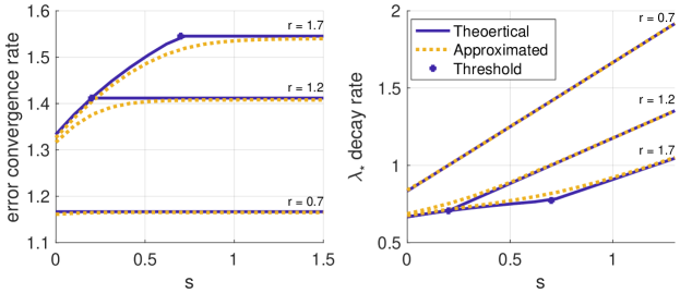
Figure 1: Over-smoothing ($s>r-\frac{\beta+1}{2}$) yields optimal convergence rate (left), at the price of fast decaying optimal hyper-parameter $\lambda_{*}$ (right). Here $s$ is the smoothness parameter of the fractional RKHS regularizer, and $r$ is the regularity of the true function, and $\beta$ represents the spectral decay of the inversion operator. See Sect.3.3 and Theorem 3.3 for details.

Notations.

The notation $X\sim\mathcal{N}(a,\Sigma)$ means that the random variable $X$ has a Gaussian distribution with mean $a$ and covariance $\Sigma$. $L^{2}_{\rho}$ denotes the function space of square-integrable functions defined on the support of the measure $\rho$. We denote by $\mathcal{L}_{{\overline{G}}}^{-1}$ the pseudo-inverse of the operator $\mathcal{L}_{{\overline{G}}}$.

Related works.

A large literature has studied convergence of regularized estimators, and we mention only those close to our setting, particularly those using explicitly the error norm to select the optimal hyper-parameter [15]. In the case of vanishing measurement error, convergence has been proven in [27, Theorem 1.1, page 8] without a rate; [10, Theorem 5.8, page 131] studies the convergence rate of the $L^{2}$-regularized estimator when the measurement error decays uniformly. Also, convergence rates with refining mesh have been studied in [28, 29, 30, 22, 18] for inverse problems. On the other hand, RKHS regularization has been widely studied in inverse problems [29, 22, 18] and learning theory (see e.g.,[6, 25, 7, 1, 4, 24]) using pre-specified reproducing kernels, where the learning in the large sample limit is a well-posed inverse problem. Additionally, small noise analysis has been used to study maximum a posterior of Bayesian inverse problems [9, 4], samplers [12], and numerical solutions to stochastic differential equations [3].

However, none of these works consider the adaptive fractional RKHS regularization introduced in this study. Neither do they discover the delicate dependence of the optimal convergence rate on the spectrum decay and the regularity of the true solution.

2 Tikhonov and RKHS regularization

2.1 Ill-posed linear inverse problems

Let $\rho$ be a probability measure with compact support $\mathcal{S}$. Consider the inverse problem:

$$\text{recover }\phi\,\text{ in }\,y=L\phi+\sigma\dot{W}\,\text{ from data }\{(L_{k},y_{k})\}_{k=1}^{n},$$ (2.1)

where $L_{k}:L^{2}_{\rho}\to\mathbb{Y}$ are bounded linear operators between the Hilbert spaces $L^{2}_{\rho}$ and $\mathbb{Y}$. Here $\dot{W}$ is a $\mathbb{Y}$-valued white noise, i.e., $\langle{\dot{W},y}\rangle_{\mathbb{Y}}\sim\mathcal{N}(0,\|y\|_{\mathbb{Y}}^{2})$ for each $y\in\mathbb{Y}$ (see [8] for Gaussian measures in infinite-dimension). We represent the strength of the noise by a positive constant $\sigma$, and our small noise analysis studies the convergence rates of the regularized estimator when $\sigma\to 0$.

We focus on ill-posed problems in $L^{2}_{\rho}$ that the mini-norm least squares estimator (LSE) is sensitive to noise in data or approximation error [22]. That is, in the variational formulation of the inverse problem, the minimal-norm minimizer of the loss function

$$\mathcal{E}(\phi):=\frac{1}{n}\sum_{k=1}^{n}\left\|L_{k}\phi-y_{k}\right\|^{2}_{\mathbb{Y}}=\frac{1}{n}\sum_{k=1}^{n}\langle{L_{k}^{*}L_{k}\phi,\phi}\rangle_{L^{2}_{\rho}}-2\langle{L_{k}^{*}y_{k},\phi}\rangle_{L^{2}_{\rho}}+\left\|y_{k}\right\|^{2}_{\mathbb{Y}}$$ (2.2)

is sensitive to the noise in the data $\{y_{k}\}$. Here $L^{*}_{k}$ denotes the adjoint of $L_{k}$. Such ill-posedness roots in the unboundedness of the inversion of the generalized data-dependent operator

$$\mathcal{L}_{{\overline{G}}}:=\frac{1}{n}\sum_{k=1}^{n}L_{k}^{*}L_{k}:L^{2}_{\rho}\to L^{2}_{\rho},$$ (2.3)

e.g., when $\mathcal{L}_{{\overline{G}}}$ is compact with positive eigenvalues converging to zero (see examples in Sect. 2.2).

To be precise, we introduce the following assumption and definitions. Note first that by definition, $\mathcal{L}_{{\overline{G}}}$ is a semi-positive self-adjoint operator, i.e., $\langle{\mathcal{L}_{{\overline{G}}}\phi,\phi}\rangle=\langle{\phi,\mathcal{L}_{{\overline{G}}}\phi}\rangle\geq 0$ for any $\phi\in L^{2}_{\rho}$.

Assumption 2.1.

The operator $\mathcal{L}_{{\overline{G}}}$ is a trace-class operator, i.e., $\sum_{i}\lambda_{i}<\infty$, where $\{\lambda_{i}\}_{i\geq 1}$ denote the positive eigenvalues of $\mathcal{L}_{{\overline{G}}}$ arranged in a descending order.

Denote $\{\psi_{i},\,\psi_{j}^{0}\}_{i,j}$ be the orthonormal eigenfunctions of $\mathcal{L}_{{\overline{G}}}$ with $\psi_{i}$ and $\psi_{j}^{0}$ corresponding to eigenvalues $\lambda_{i}$ and zero (if any). Then, $\{\lambda_{i}\}_{i\geq 1}$ is either finite or $\lambda_{i}\to 0$ as $i\to\infty$, and these eigenfunctions form a complete orthonormal basis of $L^{2}_{\rho}$.

We define the function space of identifiability as the subspace of $L^{2}_{\rho}$ in which the inverse of $\mathcal{L}_{{\overline{G}}}$ is well-defined, i.e., the loss function has a unique minimizer.

Definition 2.2 (Function space of identifiability (FSOI)).

The FSOI of the inverse problem in (2.1) is $H=\mathrm{Null}(\mathcal{L}_{{\overline{G}}})^{\perp}$, the complement of the null space of the operator $\mathcal{L}_{{\overline{G}}}$.

Definition 2.3 (Ill-posed inverse problem).

The inverse problem in (2.1) is ill-posed in $L^{2}_{\rho}$ if the operator $\mathcal{L}_{{\overline{G}}}^{-1}:H\to L^{2}_{\rho}$ is unbounded, where $H=\mathrm{Null}(\mathcal{L}_{{\overline{G}}})^{\perp}$ is the FSOI.

Note that ill-posedness differs from ill-conditionedness. An ill-conditioned problem has a large condition number $\lambda_{max}/\lambda_{min}$, where $\lambda_{max}$ and $\lambda_{min}$ are maximal and minimal positive eigenvalues of $\mathcal{L}_{{\overline{G}}}$. Thus, an ill-posed problem is always ill-conditioned, but a well-posed inverse problem can be ill-conditioned. Also, when $\mathcal{L}_{{\overline{G}}}$ is finite-rank (i.e., it has only finitely many nonzero eigenvalues), the inverse problem is well-posed.

The next lemma characterizes the mini-norm LSE, with the proof postponed to Appendix A.

Lemma 2.4 (The mini-norm LSE).

Under Assumption 2.1, the mini-norm LSE is the unique minimizer of the loss function (defined in (2.2)) in the FSOI $H$, and it can be written as

$$\widehat{\phi}=\mathcal{L}_{{\overline{G}}}^{-1}\phi^{y},\quad\phi^{y}:=\frac{1}{n}\sum_{k=1}^{n}L_{k}^{*}y_{k}.$$ (2.4)

If the true solution is $\phi_{*}$, i.e., $y_{k}=L_{k}\phi_{*}+\sigma\dot{W}_{k}$, the estimator has the following properties.

• The term $\phi^{y}$ has a decomposition

  $$\phi^{y}=\mathcal{L}_{{\overline{G}}}\phi_{*}+\phi^{\sigma},\,\text{ with }\phi^{\sigma}=\sum_{i}\sigma\xi_{i}\lambda_{i}^{1/2}\psi_{i},$$ (2.5)

  where $\{\xi_{i}\}$ are independent and identically distributed Gaussian random variables. That is, $\phi^{\sigma}\sim\mathcal{N}(0,\sigma^{2}\mathcal{L}_{{\overline{G}}})$ with $\mathbb{E}\left[{\|\phi^{\sigma}\|_{L^{2}_{\rho}}^{2}}\right]=\sigma^{2}\sum_{i}\lambda_{i}$.

• When $\sum_{i}\lambda_{i}^{-1}<\infty$, the estimator $\widehat{\phi}=\mathcal{L}_{{\overline{G}}}^{-1}\phi^{y}\sim\mathcal{N}(\phi_{*},\sigma^{2}\mathcal{L}_{{\overline{G}}}^{-1})$ is well-defined; but when $\sum_{i}\lambda_{i}^{-1}=\infty$, the pseudo-inverse $\mathcal{L}_{{\overline{G}}}^{-1}\phi^{y}$ is ill-defined in $L^{2}_{\rho}$ since $\mathbb{E}\left[{\|\mathcal{L}_{{\overline{G}}}^{-1}\phi^{y}\|_{L^{2}_{\rho}}^{2}}\right]=\infty$.

• When the data is noiseless, we have $\widehat{\phi}=\mathcal{L}_{{\overline{G}}}^{-1}\phi^{y}=P_{H}\phi_{*}$, where $P_{H}$ is the projection to $H$.

The above lemma reveals the nature of the ill-posedness, and provides insights into regularization: the inverse problem is ill-defined beyond the FSOI $H$, and it is ill-posedness in $H$ when the positive eigenvalues of $\mathcal{L}_{{\overline{G}}}$ converge to zero. As a result, when regularizing the ill-posed problem, it is important to ensure that the solution lies in the FSOI. Before introducing such regularization strategies in Sect. 2.3, we first introduce a few examples of the operator $\mathcal{L}_{{\overline{G}}}$.

2.2 Examples

As illustrations, we consider integral operators $L_{k}:L^{2}_{\nu}(\mathcal{S})\to L^{2}_{\mu}(\mathcal{T})$ with kernels $K_{k}$:

$$L_{k}\phi(t)=\int_{\mathcal{S}}K_{k}(t,s)\phi(s)\nu(ds),\,t\in\mathcal{T}.$$ (2.6)

Here $\mathcal{S}\subset\mathbb{R}$ and $\mathcal{T}\subset\mathbb{R}$ are two compact sets, which can be either intervals or sets with finitely many elements. The measure $\nu$ is a finite measure with support $\mathcal{S}$: it is the Lebesgue measure when $\mathcal{S}$ is an interval, and it is an atom measure when $\mathcal{S}$ has finitely many elements. Similarly, we let $\mu$ be a finite measure on $\mathcal{T}$. Three examples are as follows:

• Fredholm integral equations of the first kind, in which one solves $\phi$ from $(K_{1},y_{1})$:

  $$y_{1}(t)=L_{1}\phi(t)+\sigma\dot{W}(t)=\int_{\mathcal{S}}K_{1}(t,s)\phi(s)ds+\sigma\dot{W}(t),\,t\in\mathcal{T},$$ (2.7)

  where $\mathcal{S}$ and $\mathcal{T}$ are closed intervals (for example, $\mathcal{S}=[0,1]$ and $\mathcal{T}=[1,2]$) with $\nu$ and $\mu$ being the Lebesgue measure. It is a prototype of ill-posed inverse problems dating backing from Hadamard [14], and it is a testbed for regularization methods [28, 15, 18, 21].

• Learning kernels in nonlocal operators, in which one aims to recover the kernel $\phi$ in the nonlocal operator $R_{\phi}:H^{1}_{0}\to\mathbb{Y}$:

  $$y_{k}(t)=R_{\phi}[u_{k}]+\sigma\dot{W}_{k}(t),L_{k}\phi(t)=R_{\phi}[u_{k}]=\int_{\mathcal{S}}K_{k}(t,s)\phi(s)ds,\,t\in\mathcal{T}$$

  from data pairs $\{(u_{k},y_{k})\}$. Here $H^{1}_{0}$ a Sobolev space and $K_{k}$ can be $K_{k}(t,s)=\partial_{t}u_{k}(t+s)u_{k}(t)$ [17, 19] or $K_{k}(t,s)=u_{k}(t)-u_{k}(s)$ [31].

• Recovering kernels in Toeplitz matrix or Hankel matrix from data [13].

In these examples, the measure $\rho$ can be data-dependent, $\frac{d\rho}{d\nu}(s):=\frac{1}{Z}\sum_{k=1}^{n}\int_{\mathcal{T}}|K_{i}(t,s)|\mu(dt),\,\forall s\in\mathcal{S}$, where $Z$ is a normalizing constant, or one can use the Lebesgue measure on the support of $\rho$ for simplicity. The operator $\mathcal{L}_{{\overline{G}}}$ in (2.3) is determined by the bilinear form $\langle{\mathcal{L}_{{\overline{G}}}\phi,\psi}\rangle=\frac{1}{n}\sum_{k=1}^{n}\langle{L_{k}\phi,L_{k}\psi}\rangle_{{L^{2}_{\mu}(\mathcal{T})}}=\int_{\mathcal{S}}\int_{\mathcal{S}}\phi(s)\psi(s^{\prime}){\overline{G}}(s,s^{\prime})\rho(ds)\rho(ds^{\prime})$, where the bivariate function ${\overline{G}}:\mathcal{S}\times\mathcal{S}\to\mathbb{R}$ is defined as

$${\overline{G}}(s,s^{\prime}):=\frac{1}{\frac{d\rho}{d\nu}(s)\frac{d\rho}{d\nu}(s^{\prime})}\int_{\mathcal{T}}\frac{1}{n}\sum_{k=1}^{n}K_{k}(t,s)K_{k}(t,s^{\prime})\mu(dt).$$

In fact, $\mathcal{L}_{{\overline{G}}}$ is an integral operator with ${\overline{G}}$ as its kernel, i.e. $\mathcal{L}_{{\overline{G}}}\phi(r):=\int_{a}^{b}\phi(s){\overline{G}}(r,s)\rho(ds)$. The function ${\overline{G}}$ is a Mercer kernel when the functions $K_{k}:\mathcal{T}\times\mathcal{S}\to\mathbb{R}$ are continuous. Hence, it defines an RKHS, $H_{G}=\mathcal{L}_{{\overline{G}}}^{1/2}(L^{2}_{\rho})$. The FSOI is the closure of this RKHS in $L^{2}_{\rho}$ (see [20]).

2.3 Tikhonov and RKHS regularization

We introduce a class of adaptive fractional RKHSs for regularization that can ensure the optimization search takes place inside the data-dependent FSOI. These RKHSs are constructed through the eigen-decomposition of the operator $\mathcal{L}_{{\overline{G}}}$, having a parameter $s$ controlling the smoothness.

Definition 2.5 (Fractional RKHS).

For $s\geq 0$, the $s$-fractional RKHS associated with operator $\mathcal{L}_{{\overline{G}}}$ in $L^{2}_{\rho}$ is $H^{s}_{G}=\mathcal{L}_{{\overline{G}}}^{s/2}(L^{2}_{\rho})$, with norm $\|\phi\|_{H^{s}_{G}}^{2}=\|\mathcal{L}_{{\overline{G}}}^{-s/2}\phi\|_{L^{2}_{\rho}}^{2}$ for all $\phi=\sum_{i:\lambda_{i}>0}c_{i,\phi}\psi_{i}$ such that $\sum_{i}\lambda_{i}^{-s}c_{i,\phi}^{2}<\infty$, where $\{(\lambda_{i},\psi_{i})\}$ are the positive eigenvalue and eigenfunction pairs of $\mathcal{L}_{{\overline{G}}}$.

These fractional RKHS recovers the RKHS in DARTR in [20] when $s=1$. Also, when $s=0$, the fractional RKHS is $H_{G}^{0}=H$, the FSOI.

Now we use the norms of these fractional RKHSs for regularization:

$$\widehat{\phi}_{\lambda}^{s}=\underset{\phi\in H_{G}^{s}}{\operatorname{arg}\operatorname{min}}\;\mathcal{E}_{\lambda}(\phi):=\mathcal{E}(\phi)+\lambda\left\|\phi\right\|_{H_{G}^{s}}^{2}.$$ (2.8)

The next proposition presents the $H_{G}^{s}$-regularized estimator and its $L^{2}_{\rho}$ error.

Proposition 2.6 (Fractional RKHS regularized estimator).

The minimizer in (2.8) is

$$\widehat{\phi}_{\lambda}^{s}=(\mathcal{L}_{{\overline{G}}}+\lambda\mathcal{L}_{{\overline{G}}}^{-s})^{-1}\phi^{y},$$ (2.9)

Let the true function be $\phi_{*}=\sum_{i}c_{i}\psi_{i}+\sum_{j}d_{j}\psi_{j}^{0}$, where $\{\psi_{i},\,\psi_{j}^{0}\}_{i,j}$ denote the orthonormal eigenfunctions of $\mathcal{L}_{{\overline{G}}}$ with $\psi_{i}$ and $\psi_{j}^{0}$ corresponding to eigenvalues $\lambda_{i}$ and zero (if any). Then, for any $\lambda>0$, the error of this regularized estimator is

$$\|\widehat{\phi}_{\lambda}^{s}-\phi_{*}\|^{2}_{L^{2}_{\rho}}=\sum_{i}(\lambda_{i}+\lambda\lambda_{i}^{-s})^{-2}(\sigma\lambda_{i}^{1/2}\xi_{i}-\lambda c_{i})^{2}+\sum_{j}d_{j}^{2},$$ (2.10)

where $\xi_{i}$ are iid standard Gaussian. In particular, when $\sum_{j}d_{j}^{2}=0$, the expectation of the error is

$$e(\lambda;s)= \mathbb{E}\|\widehat{\phi}_{\lambda}-\phi_{*}\|^{2}_{L^{2}_{\rho}}=\sum_{i}(\lambda_{i}^{s+1}+\lambda)^{-2}(\sigma^{2}\lambda_{i}^{2s+1}+\lambda^{2}c_{i}^{2}).$$ (2.11)

Proof.

The uniqueness of the minimizers and their explicit form follow from the Fréchet derivatives of the regularized loss function. In fact, note that $\|\phi\|_{H_{G}^{s}}=\langle{\mathcal{L}_{{\overline{G}}}^{-s}\phi,\psi}\rangle_{L^{2}_{\rho}}$ since the operator $\mathcal{L}_{{\overline{G}}}^{s/2}$ is self-adjoint. Then, similar to (A.2), the Fréchet derivative of $\mathcal{E}_{\lambda}$ at $\phi\in H_{G}^{s}$ under the $L^{2}_{\rho}$-topology is

$$\nabla\mathcal{E}_{\lambda}(\phi)=2[(\mathcal{L}_{{\overline{G}}}+\lambda\mathcal{L}_{{\overline{G}}}^{-s})\phi-\phi^{y}].$$

Then, its unique zero in $H_{G}^{s}$ is $\widehat{\phi}_{\lambda}^{s}=(\mathcal{L}_{{\overline{G}}}+\lambda\mathcal{L}_{{\overline{G}}}^{-s})^{-1}\phi^{y}$.

To obtain the eigenvalue characterizations of the error, recall the decomposition $\phi^{y}=\mathcal{L}_{{\overline{G}}}\phi_{*}+\phi^{\sigma}$ in (2.5). Then, we obtain (2.10) by noticing that

$$\widehat{\phi}_{\lambda}^{s} =(\mathcal{L}_{{\overline{G}}}+\lambda\mathcal{L}_{{\overline{G}}}^{-s})^{-1}(\mathcal{L}_{{\overline{G}}}{\phi_{*}}+\lambda\mathcal{L}_{{\overline{G}}}^{-s}\phi_{*}-\lambda\mathcal{L}_{{\overline{G}}}^{-s}\phi_{*}+\phi^{\sigma})$$

$$=\phi_{*}+(\mathcal{L}_{{\overline{G}}}+\lambda\mathcal{L}_{{\overline{G}}}^{-s})^{-1}(-\lambda\phi_{*}+\phi^{\sigma}).$$ (2.12)

Additionally, using the fact that $\phi^{\sigma}=\sum_{i}\sigma\lambda_{i}^{1/2}\xi_{i}$ with $\xi_{i}$ being iid standard Gaussian, we obtain (2.11) by taking expectation.

Note that when $s=0$, this regularization reduces to the conventional $L^{2}$-Tikhonov regularization but with the minimization search constrained inside the FSOI. When $s=1$, it recovers the DARTR.

Proposition 2.6 demonstrates the complexity of choosing an optimal hyper-parameter $\lambda$. An optimal $\lambda$ minimizing the error in (2.10) must balance the error caused by the noise and the bias caused by the regularization. It depends on the spectrum of the operator, the true solution (which may have non-identifiable components outside the FSOI), and the realization of the noise. In particular, the dependence on the realization of the noise makes the analysis of the regularized estimator intractable. Thus, we consider the expectation of the error in (2.11) in our small noise analysis in the next section, and seek an optimal $\lambda$ to achieve a tradeoff between the bias $\mathbb{E}\|(\mathcal{L}_{{\overline{G}}}+\lambda\mathcal{L}_{{\overline{G}}}^{-s})^{-1}(-\lambda\phi_{*})\|_{L^{2}_{\rho}}^{2}$ caused by regularization and the variance $\mathbb{E}\|(\mathcal{L}_{{\overline{G}}}+\lambda\mathcal{L}_{{\overline{G}}}^{-s})^{-1}(\phi^{\sigma})\|_{L^{2}_{\rho}}^{2}$ caused by the noise.

3 Small noise analysis for regularized estimators

We introduce a small noise analysis framework that studies the convergence of the regularized estimator in the small noise limit. We show first that the fractional RKHS regularizer removes the bias outside the FSOI, thus leading to estimators with vanishing errors, whereas the conventional $L^{2}$ Tikhonov regularizer cannot. Thus, when studying convergence rates, we don’t consider the conventional $L^{2}$-regularizer and only compare the fractional RKHS regularizers with different smoothness parameters $s$. We will show that over-smoothing by the fractional RKHSs always leads to optimal convergence rates.

3.1 Finite-rank operators: removing bias outside the FSOI

We show that the conventional $L^{2}$ Tikhonov regularizer has the drawback of not removing the perturbation outside the FSOI (often caused by numerical error and/or model error), leading to an estimator failing to converge in the small noise limit. In contrast, the fractional RKHS regularizer removes the bias outside the FSOI, consistently leading to convergent estimators.

Proposition 3.1.

Assume that the operator is finite rank, the true function is inside the FSOI, and a presence of perturbations outside the FSOI as follows:

• the operator $\mathcal{L}_{{\overline{G}}}$ has descending eigenvalues satisfying $\lambda_{i}=0$ for all $i>K$ and $\lambda_{K}>0$;

• the term $\phi^{y}$ in (2.4) is approximated by $\widetilde{\phi}^{y}$ such that $\widetilde{\phi}^{y}=\phi^{y}+\phi^{\epsilon}$ with $\phi^{\epsilon}\in\mathrm{null}(\mathcal{L}_{{\overline{G}}})$;

• the true function $\phi_{*}=\sum_{1\leq i\leq K}c_{i}\psi_{i}$, where $\{\psi_{i}\}$ are the eigen-functions of $\{\lambda_{i}\}$.

Then, when $\sigma\to 0$, the conventional $L^{2}$-regularized estimator $\widetilde{\phi}_{\lambda}^{L^{2}}=(\mathcal{L}_{{\overline{G}}}+\lambda I)^{-1}\widetilde{\phi}^{y}$ has a non-vanishing bias; in contrast, the fractional RKHS regularized estimator $\widetilde{\phi}_{\lambda}^{s}=(\mathcal{L}_{{\overline{G}}}+\lambda\mathcal{L}_{{\overline{G}}}^{-s})^{-1}\widetilde{\phi}^{y}$ has a vanishing bias.

Proof.

Let $\phi^{\epsilon}=\sum_{i>K}\epsilon_{i}\psi_{i}$ with $0<\|\phi^{\epsilon}\|_{L^{2}_{\rho}}^{2}=\sum_{i>K}\epsilon_{i}^{2}<\infty$. Then, applying the decomposition (2.12), we have

$$\mathbb{E}[\|\widetilde{\phi}_{\lambda}^{L^{2}}-\phi_{*}\|_{L^{2}_{\rho}}^{2}] =\sum_{1\leq i\leq K}(\lambda_{i}+\lambda)^{-2}(\sigma^{2}\lambda_{i}+\lambda^{2}c_{i}^{2})+\lambda^{-2}\sum_{i>K}\epsilon_{i}^{2}.$$

Using the fact that $(\lambda_{i}+\lambda)^{-2}(\sigma^{2}\lambda_{i}+\lambda^{2}c_{i}^{2})\geq(\lambda_{i}+\lambda)^{-2}\lambda^{2}c_{i}^{2}\geq\lambda_{K}^{-2}\lambda^{2}c_{i}^{2}$, we obtain

$$\mathbb{E}[\|\widetilde{\phi}_{\lambda}^{L^{2}}-\phi_{*}\|_{L^{2}_{\rho}}^{2}]\geq\lambda^{2}K\lambda_{K}^{-2}\sum_{1\leq i\leq K}c_{i}^{2}+\lambda^{-2}\|\phi^{\epsilon}\|_{L^{2}_{\rho}}^{2}\geq 2\sqrt{K}\lambda_{K}^{-1}\|\phi_{*}\|_{L^{2}_{\rho}}\|\phi^{\epsilon}\|_{L^{2}_{\rho}},$$

where the last inequality follows from that fact that $\min_{x>0}ax+x^{-1}b\geq 2\sqrt{ab}$. Hence, the conventional $L^{2}$-regularizer’s estimator has a non-vanishing bias.

Similarly, the $H_{G}^{s}$-regularizer’s estimator has an expected bias:

$$\mathbb{E}[\|\widetilde{\phi}_{\lambda}^{s}-\phi_{*}\|_{L^{2}_{\rho}}^{2}]=\sum_{1\leq i\leq K}(\lambda_{i}^{s+1}+\lambda)^{-2}(\sigma^{2}\lambda_{i}^{2s+1}+\lambda^{2}c_{i}^{2}).$$

Hence, the minimal bias is less than its value with $\lambda=\sigma$:

$$\min_{\lambda>0}\mathbb{E}[\|\widetilde{\phi}_{\lambda}^{L^{2}}-\phi_{*}\|_{L^{2}_{\rho}}^{2}]\leq\mathbb{E}[\|\widetilde{\phi}_{\sigma}^{s}-\phi_{*}\|_{L^{2}_{\rho}}^{2}]$$

$$= \sum_{1\leq i\leq K}(\lambda_{i}^{s+1}+\sigma)^{-2}\sigma^{2}(\lambda_{i}^{2s+1}+c_{i}^{2})\leq\sigma^{2}\lambda_{K}^{-2s-2}(K\lambda_{1}^{2s+1}+\|\phi_{*}\|_{L^{2}_{\rho}}^{2}).$$

Consequently, this bias vanishes as $\sigma\to 0$.

3.2 Infinite-rank operator: convergence rate

We analyze the convergence rate of the regularized estimators as $\sigma\downarrow 0$. The focus is on the dependence of the rate on the smoothness parameter $s$ of $H_{G}^{s}$ and the regularity of the true function.

Assumption 3.2.

Assume the following spectrum decay of $\mathcal{L}_{{\overline{G}}}$ and smoothness of the true function:

• (Spectrum decay). The eigenvalues of $\mathcal{L}_{{\overline{G}}}$ have either exponential or polynomial decay, i.e.,

  $$\lambda_{i}=p_{i}^{-1}f(i),$$ (3.1)

  where $f$ is either exponential, $f(x)=e^{-\theta(x-1)}$ with $\theta>0$, or polynomial, $f(x)=x^{-\theta}$ with $\theta>1$. Here $\{p_{i}\}$ are perturbations satisfying $0<a\leq p_{i}^{-1}\leq b<\infty$ for each $i$.

• (r-smoothness of $\phi_{*}$). Let $\phi_{*}=\sum_{i}c_{i}\psi_{i}\in L^{2}_{\rho}$ be $r$-smooth with respect to the spectrum in the sense that $|c_{i}|=\lambda_{i}^{r}$, where $r>0$ when $f$ is exponential and $r>\frac{1}{2\theta}$ when $f$ is polynomial.

We define a constant $\beta$ to unify notation for both exponential and polynomial spectrum decay:

$$\beta=\begin{cases}1,&\text{ if }f(x)=e^{-\theta(x-1)};\\ \theta^{-1}+1,&\text{ if }f(x)=x^{-\theta}.\end{cases}$$ (3.2)

Our main results are the convergence rates of the $H_{G}^{s}$- regularized estimators in the small noise limit.

Theorem 3.3 (Convergence rates of regularized estimators).

Suppose Assumption 3.2 holds and recall the $H_{G}^{s}$-regularizer’s error $e(\lambda,s)$ in (2.11). Then, the optimal parameter $\lambda_{*}=\underset{\lambda>0}{\operatorname{arg}\operatorname{min}}\;e(\lambda;s)$ and the estimator’s error converge as $\sigma\to 0$ in the following orders:

$$\lambda_{*}\simeq\begin{cases}\sigma^{\frac{2s+2}{2r+1}},&s>r-\frac{\beta+1}{2},\\ \sigma^{\frac{2s+2}{2s+2+\beta}},&s<r-\frac{\beta+1}{2};\end{cases}\quad e(\lambda_{*};s)\simeq\begin{cases}\sigma^{2-\frac{2\beta}{2r+1}},&s>r-\frac{\beta+1}{2},\\ \sigma^{2-\frac{2\beta}{2s+2+\beta}},&s<r-\frac{\beta+1}{2},\end{cases}$$ (3.3)

where $\beta$ is the constant defined in (3.2).

We introduce a generic small noise analysis scheme to compute the rates. It extends the classical idea of bias-variance trade-off in learning theory [6, 7] to ill-posed inverse problems. A key component is an integral approximation of the series under Assumption 3.2 to reveal the dominating orders, making it possible to compute the optimal hyper-parameter $\lambda$ through an algebraic equation. The scheme consists of three steps:

• Reduce the selection of optimal $\lambda$ to solving an algebraic equation;

• Estimate the dominating orders of the series for small $\lambda$ by integrals.

• Solve the algebraic equation and compute the optimal rates.

This scheme was used in [29] to study the rates when the mesh size vanishes. Our innovation is a systematic formulation for the study of small noise limits.

Step 1 follows by separating the variance and bias terms and solving the equation for a critical point, as shown in Lemma 3.4.

Lemma 3.4.

For each $s\geq 0$, the minimizer $\lambda_{*}:=\underset{\lambda>0}{\operatorname{arg}\operatorname{min}}\;e(\lambda,s)$ satisfies

$$\lambda=-\sigma^{2}\frac{A^{\prime}(\lambda;s)}{2B_{1}(\lambda;s)},$$ (3.4)

where $A^{\prime}(\lambda,s)$ and $B_{1}(\lambda,s)$ are series determined by the spectrum and $r$ in Assumption 3.2:

$$-\frac{1}{2}A^{\prime}(\lambda;s)=\sum_{i}(\lambda_{i}^{s+1}+\lambda)^{-3}\lambda_{i}^{2s+1},\quad B_{1}(\lambda;s)=\sum_{i}(\lambda_{i}^{s+1}+\lambda)^{-3}\lambda_{i}^{s+1+2r}.$$

Proof.

Rewrite (2.11) to separate the variance and bias terms as

$$e(\lambda;s) =\sigma^{2}A(\lambda;s)+\lambda^{2}B(\lambda;s),\text{ where }$$ (3.5)

$$A(\lambda;s)=\sum_{i}(\lambda_{i}^{s+1} +\lambda)^{-2}\lambda_{i}^{2s+1},\quad B(\lambda;s)=\sum_{i}(\lambda_{i}^{s+1}+\lambda)^{-2}\lambda_{i}^{2r}.$$ (3.6)

Then for each $s$, the minimizer $\lambda_{*}$ must satisfy the equation for a critical point:

$$0=\frac{d}{d\lambda}e(\lambda;s)=\sigma^{2}A^{\prime}(\lambda;s)+2\lambda[B(\lambda;s)+\frac{\lambda}{2}B^{\prime}(\lambda;s)].$$

Setting $B_{1}(\lambda;s)=B(\lambda;s)+\frac{\lambda}{2}B^{\prime}(\lambda;s)$, we obtain Equ. (3.4). The series for $A^{\prime}$ and $B_{1}$ follows from (3.6) and the derivatives of these terms.

In Step 2, we estimate the dominating terms of $A^{\prime}$ and $B_{1}$ for small $\lambda$ (since it will decay with $\sigma$), which requires estimating the dominating terms in $A,B$ and $B^{\prime}$ in (3.6). All these series can be written in the general form of parameterized series:

$$F_{s}(\lambda;k,\alpha):=\sum_{i=1}^{\infty}(\lambda_{i}^{s+1}+\lambda)^{-k}\lambda_{i}^{\alpha},$$

where $k\in\{2,3\}$ and $\alpha\in\{(2s+1),(s+1+2r),2r\}$. For example, $A(\lambda;s)=F_{s}(\lambda;2,2s+1)$ and $B(\lambda;s)=F_{s}(\lambda;2,2r)$. We provide a general estimation for series $F_{s}(\lambda;k,\alpha)$ for all $k>0$, $\alpha\geq 1$ and $s\geq 0$ in Lemma A.1, which is of independent interest by itself. The basic idea in its proof is to approximate the series by Riemann sum. In particular, these series estimations provide dominating terms in the series $A,A^{\prime},B$ and $B_{1}$ when $\lambda$ is small, as shown in the next lemma. Both lemmas are technical and their proofs can be found in Appendix A. We will use the big-O notation to denote the approximation error and highlight the dominating terms.

Lemma 3.5.

Under the Assumption 3.2, as $\lambda\to 0$, we have

$$A(\lambda;s) =C_{A}\lambda^{-\eta_{A}}+O(1),\quad\frac{-1}{2}A^{\prime}(\lambda;s)=C_{A^{\prime}}\lambda^{-\eta_{A}-1}+O(1),$$ (3.7)

$$B_{1}(\lambda;s) =\begin{cases}C_{B_{1}}\lambda^{-\eta_{B}}+O(1),&\\ C_{B_{1}}+O(1),&\end{cases}B(\lambda;s)=\begin{cases}C_{B}\lambda^{-\eta_{B}}+O(1),&s>r-\frac{\beta+1}{2}\\ C_{B}+O(1),&s<r-\frac{\beta+1}{2}\end{cases},$$

where $\eta_{A}=\frac{\beta}{s+1}$, $\eta_{B}=\frac{\beta-2r-1}{s+1}+2$. Here $C_{A^{\prime}},C_{A},C_{B^{\prime}},C_{B}>0$ are constants independent of $\lambda$.

In Step 3, we prove Theorem 3.3 by solving the algebraic equations and computing the rates.

Proof of Theorem 3.3.

When $r<s+\frac{\beta+1}{2}$, by (3.4) and the estimates in Lemma 3.5, the minimizer $\lambda_{*}$ satisfies $\lambda=2\sigma^{2}\frac{C_{A^{\prime}}\lambda^{-\eta_{A}-1}+O(1)}{C_{B_{1}}\lambda^{-\eta_{B}}+O(1)},$ where $\eta_{A}=\frac{\beta}{s+1}$ and $\eta_{B}=\frac{\beta-2r-1}{s+1}+2$. Hence $\eta_{A}+2>\eta_{A}-\eta_{B}+2=\frac{2r+1}{s+1}>0$ and

$$\lambda^{\eta_{A}-\eta_{B}+2}+O(\lambda^{\eta_{A}+2})=2C_{A^{\prime}}{C_{B_{1}}}^{-1}\sigma^{2}(1+O(\lambda^{\eta_{A}+1}))$$

when $\sigma\to 0$. Solving from the dominating terms, we obtain $\lambda_{*}\simeq c\sigma^{\frac{2s+2}{2r+1}}$ with $c=\left(\frac{2C_{A^{\prime}}}{C_{B_{1}}}\right)^{\frac{s+1}{2r+1}}$.

The optimal $\lambda_{*}$, together with (3.5) and the estimates in Lemma 3.5, imply that

$$e(\lambda_{*};s) =\sigma^{2}A(\lambda_{*};s)+\lambda_{*}^{2}B(\lambda_{*s};s)\simeq\sigma^{2}\lambda_{*}^{-\eta_{A}}C_{A}+\lambda_{*}^{2-\eta_{B}}C_{B}$$

$$=c^{-\eta_{A}}\sigma^{2+\frac{2s+2}{2r+1}(-\eta_{A})}C_{A}+c^{2-\eta_{B}}\sigma^{\frac{2s+2}{2r+1}(2-\eta_{B})}C_{B}.$$

Notice that $2+\frac{2s+2}{2r+1}(-\eta_{A})=\frac{2s+2}{2r+1}(2-\eta_{B})=2-\frac{\beta}{2r+1}$, hence, $e(\lambda_{*};s)\simeq C\sigma^{2-\frac{2\beta}{2r+1}},$where $C=c^{-\eta_{A}}C_{A}+c^{2-\eta_{B}}C_{B}$.

When $r>s+\frac{\beta+1}{2}$, $\lambda_{*}$ satisfies $\lambda=2\sigma^{2}\frac{C_{A^{\prime}}\lambda^{-1-\eta_{A}}+O(1)}{C_{B_{1}}+O(1)}.$ As $\sigma\to 0$, notice that $\frac{2}{\eta_{A}+2}=\frac{2s+2}{2s+2+\beta}$, we have $\lambda_{*}\simeq c\sigma^{\frac{2s+2}{2s+2+\beta}}$ with $c=\left(\frac{2C_{A^{\prime}}}{C_{B_{1}}}\right)^{\frac{s+1}{2s+2+\beta}}$. Hence,

$$e(\lambda_{*};s)=c^{-\eta_{A}}\sigma^{2+\frac{2s+2}{2s+2+\beta}(-\eta_{A})}C_{A}+c^{2-\eta_{B}}\sigma^{\frac{4s+4}{2s+2+\beta}}C_{B}.$$

Again, noticing that $2+\frac{2s+2}{2s+2+\beta}(-\eta_{A})=\frac{4s+4}{2s+2+\beta}=2-\frac{\beta}{2s+2+\beta}$, we obtain $e(\lambda_{*};s)=C\sigma^{2-\frac{\beta}{2s+2+\beta}}$, where $C=c^{-\eta_{A}}C_{A}+c^{2-\eta_{B}}C_{B}$.

Remark 3.6.

The convergence rate at the threshold $s=r-\frac{\beta+1}{2}$ is not covered by Theorem 3.3, because it requires a solution of a non-algebraic equation involving logarithmic terms.

3.3 Numerical Examples

Oracle rates under exponential spectral decay. Fig. 1 demonstrates the dependence of optimal convergence rate on the $s$ and $r$. In the left figure, the theoretical rates (denoted by “Theoretical”) in Theorem 3.3 are close to the numerically approximated rates (“Approximated”). They differ the most near the thresholds $r-\frac{\beta+1}{2}$, which is not covered by the theorem (see Remark 3.6). Both show that over-smoothing leads to optimal convergence rates. However, as the right figure shows, the optimal hyper-parameter decays at a rate increasing with $s$, making it difficult to select in practice.

The settings for the approximated rates are as follows. We take the spectrum to be $f(x)=e^{-1.5x}$ evaluated at $i\in\{1,\ldots,200\}$, and $r\in\{0.7,1.2,1.7\}$. We select the optimal $\lambda_{*}$ to be the minimizer of $e(\lambda;s)$ in (2.11) in the range $[10^{-25},10^{2}]$ with true $\phi$ known, and then compute $e(\lambda_{*};s)$. We compute the rate of $\lambda_{*}$ and $e(\lambda_{*};s)$ with $\sigma\in[10^{-7},10^{-1}]$.

Rates with L-curve selected $\lambda_{*}$.

Consider the Fredholm integral equation (2.7) with kernel $K_{1}(x,y)=\begin{cases}-\frac{\sin 2(1-y)\sin 2x}{2\sin 2},\ 0\leq x\leq y\leq 1,\\ -\frac{\sin 2(1-x)\sin 2y}{2\sin 2},\ 0\leq y\leq x\leq 1.\\ \end{cases}$Note that $K_{1}$ is the Green’s function of the equation $u(x)^{\prime\prime}+4u(x)=f(x),\ x\in(0,1),\ u(0)=u(1)=0$. We take $\rho$ to be the Lebesgue measure on $[0,1]$ and set $\mathbb{Y}=L^{2}([0,1])=L^{2}_{\rho}$. Direct computation shows that $\mathcal{L}_{{\overline{G}}}$ has eigenvalues $2(4-n^{2}\pi^{2})^{-2}$ with eigenfunctions $\phi_{n}(x)=\sin(n\pi x)$. That is, its spectrum has polynomial decay with $\theta=4$, so $\beta=\frac{5}{4}$. We evaluate the kernel in $[0,1]$ with $500$ even-spaced mesh points and take the true function $\phi=\sum_{n=1}^{N}v_{n}\lambda_{n}^{r}\phi_{n}$ with $r=1.5$ and $\{v_{n}\}$ uniformly sampled in $[-1.05,-0.95]\cup[0.95,1.05]$. We estimate $\phi$ from noisy observations with $\sigma\in[10^{-3},10^{-0.5}]$ and $H_{G}^{s}$-regularization with $s\in\{0,1,2\}$. We test two approaches estimating $\lambda_{*}$: using the L-curve method [16] (denoted by “L-curve $\lambda_{*}$") and using the true function $\phi$ (denoted by “oracle $\lambda_{*}$").

Fig. 2 shows the errors (Left) and the estimated hyper-parameters (Right) as $\sigma$ decays. As $s$ increases, the errors with L-curved estimated $\lambda_{*}$ (solid lines) first drop then increase, whereas the errors with oracle $\lambda_{*}$ decay steadily. In particular, for over-smoothed regularization with $s=2$, the optimal $\lambda_{*}$ selected by the L-curve method is unstable (Right), leading to large oscillating errors. However, for properly-smoothed regularization with $s=1$, the L-curve $\lambda_{*}$’s are close to the oracle ones and lead to estimators that are significantly more accurate than those with $s=0$ or $s=2$. Note that the threshold is $r-\frac{\beta+1}{2}=0.375$. Hence $s=1$ is big enough to have the optimal error rate.

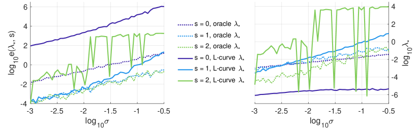
Figure 2: Over-smoothing ($s=2$) makes it difficult to select the optimal $\lambda_{*}$ by the L-curve method (right), leading to a relatively large error (left). However, when properly regularized with $s=1$, the L-curve $\lambda_{*}$’s are close to the oracle ones and lead to estimators that are significantly more accurate than those with $s=0$ or $s=2$.

3.4 Limitations

The small noise analysis does not tackle the practical selection of hyper-parameters. Its goal is to understand the fundamental role of regularization norms. Thus, it uses the oracle optimal hyper-parameters so as to focus on comparing the norms. However, it provides insights into the future projects of selecting regularization norms in conjunction with the hyper-parameters.

Also, the small noise analysis does not apply to non-Hilbert norms, particularly the $L^{1}$-norm; it is potentially applicable to other Hilbert norms, such as the $H_{0}^{1}$-norm and those non-diagonalizable in the orthonormal basis of the inversion operator, which we leave in future work.

Additionally, it is yet to extend this framework to analyze the convergence of the regularized estimator when the data size increase (i.e., either the sample size increases or the data mesh increases).

At last, this study focuses on linear inverse problems. An extension to nonlinear inverse problems requires varying second-order Fréchet derivatives of the loss function, which is beyond the scope of this study.

4 Conclusion

We have established a small noise analysis framework to understand the fundamental role of regularization norms, setting a step forward for the anatomy of regularization. For ill-posed linear inverse problems, we have introduced a class of adaptive fractional RKHS norms for regularization. Our analysis shows that over-smoothing by the fractional RKHS always leads to an optimal convergence rate, but the resulting fast decaying optimal hyper-parameter becomes difficult to select in practice.

Appendix A Technical proofs

Proof of Lemma 2.4.

The mini-norm LSE is a minimizer of the loss function. We first show that the estimator in (2.4) is the unique minimizer of the loss function $\mathcal{E}$ in $H$, i.e., it is the unique zero of the Fréchet derivative of $\mathcal{E}$ in $H$. By (2.2) and (2.3)–(2.4), we can write the loss functional as

$$\mathcal{E}(\phi)=\langle{\mathcal{L}_{{\overline{G}}}\phi,\phi}\rangle_{L^{2}_{\rho}}+\langle{\phi^{y},\phi}\rangle_{L^{2}_{\rho}}+C_{y}$$ (A.1)

with $C_{y}=\frac{1}{n}\sum_{k=1}^{n}\|y_{k}\|_{\mathbb{Y}}^{2}$. Then, the Fréchet derivative $\nabla\mathcal{E}(\phi)$ in $L^{2}_{\rho}$ is

$$\langle{\nabla\mathcal{E}(\phi),\psi}\rangle_{L^{2}_{\rho}}=\lim_{h\to 0}\frac{\mathcal{E}(\phi+h\psi)-\mathcal{E}(\phi)}{h}=\langle{2(\mathcal{L}_{{\overline{G}}}\phi-\phi^{y}),\psi}\rangle_{L^{2}_{\rho}},\,\forall\psi\in L^{2}_{\rho},$$ (A.2)

that is, $\nabla\mathcal{E}(\phi)=2(\mathcal{L}_{{\overline{G}}}\phi-\phi^{y})$. Hence, by the definition of $H$, the estimator in (2.4) is the unique zero of $\nabla\mathcal{E}(\phi)$ in $H$. Additionally, note that any LSE can be written as $\phi_{LSE}=\widehat{\phi}+\phi_{null}\in H\oplus\mathrm{Null}(\mathcal{L}_{{\overline{G}}})$. Thus, the estimator $\widehat{\phi}$ is the mini-norm LSE.

Next, we prove the estimator’s properties. For Part (a), by the definition of $\phi^{y}$, we have

$$\phi^{y}=\frac{1}{n}\sum_{k=1}^{n}L_{k}^{*}(L_{k}\phi_{*}+\sigma\dot{W}_{k})=\mathcal{L}_{{\overline{G}}}\phi_{*}+\phi^{\sigma},\quad\phi^{\sigma}=\sigma\frac{1}{n}\sum_{k=1}^{n}L_{k}^{*}\dot{W}_{k}.$$

The distribution of $\phi^{\sigma}$ is $\mathcal{N}(0,\sigma^{2}\mathcal{L}_{{\overline{G}}})$ because for each $\psi\in L^{2}_{\rho}$, the random variable $\langle{\psi,\phi^{\sigma}}\rangle_{L^{2}_{\rho}}=\frac{1}{n}\sum_{k=1}^{n}\langle{L\psi,\sigma\dot{W}_{k}}\rangle_{\mathbb{Y}}$ is Gaussian with mean zero and variance $\sigma^{2}\langle{\psi,\mathcal{L}_{{\overline{G}}}\psi}\rangle_{L^{2}_{\rho}}$ . Therefore, we can write $\phi^{\sigma}=\sum_{i}\sigma\xi_{i}\lambda_{i}^{1/2}\psi_{i}$ with $\{\xi_{i}\}$ being i.i.d. standard Gaussian, and $\mathbb{E}\left[{\|\phi^{\sigma}\|_{L^{2}_{\rho}}^{2}}\right]=\sigma^{2}\sum_{i}\lambda_{i}$, where the sum is finite by Assumption 2.1.

Part $(b)$: note that $\mathcal{L}_{{\overline{G}}}^{-1}\phi^{\sigma}=\sum_{i:\lambda_{i}>0}\lambda_{i}^{-1/2}\sigma\xi_{i}\psi_{i}$. Then, when $\sum_{i}\lambda_{i}^{-1}<\infty$ (which happens only when there are finitely many non-zero eigenvalues), we have $\mathcal{L}_{{\overline{G}}}^{-1}\phi^{\sigma}\in L^{2}_{\rho}$ because $\mathbb{E}\left[{\|\mathcal{L}_{{\overline{G}}}^{-1}\phi^{\sigma}\|_{L^{2}_{\rho}}^{2}}\right]=\sigma^{2}\sum_{i}\lambda_{i}^{-1}<\infty$. Then, $\mathcal{L}_{{\overline{G}}}^{-1}\phi^{\sigma}\sim\mathcal{N}(0,\sigma^{2}\mathcal{L}_{{\overline{G}}}^{-1})$ and the distribution of the estimator follows. But when $\sum_{i}\lambda_{i}^{-1}=\infty$, we have $\mathbb{E}\left[{\|\mathcal{L}_{{\overline{G}}}^{-1}\phi^{\sigma}\|_{L^{2}_{\rho}}^{2}}\right]=\sum_{i}\lambda_{i}^{-1}\sigma^{2}=\infty$, and hence $\mathcal{L}_{{\overline{G}}}^{-1}\phi^{y}$ is ill-defined.

For Part (c), when the data is noiseless, we have $\phi^{y}=\mathcal{L}_{{\overline{G}}}\phi_{*}$. Hence $\widehat{\phi}=\mathcal{L}_{{\overline{G}}}^{-1}\phi^{y}=P_{H}\phi_{*}$.

Lemma A.1 (Series estimation).

Assume that the sequence $\lambda_{i}$ satisfies (3.1), where $f(x)=e^{-\theta(x-1)}$ or $f(x)=x^{-\theta}$ with $\theta>1$. Then, for all $k>0$, $\alpha\geq 1$ and $s\geq 0$, as $\lambda\to 0$, we have

$$F_{s}(\lambda;k,\alpha)=\sum_{i=1}^{\infty}(\lambda_{i}^{s+1}+\lambda)^{-k}\lambda_{i}^{\alpha}=CJ(\lambda)+O(1),$$ (A.3)

where $C=\frac{C_{1}^{(s+1)k}C_{2}^{-\alpha}}{\theta}$ with constants $C_{1},C_{2}\in[b^{-1},a^{-1}]$ and

$$J(\lambda)\simeq\begin{cases}\frac{c^{\gamma-k}}{s+1}\frac{\Gamma(\gamma)\Gamma(k-\gamma)}{\Gamma(k)}\lambda^{\gamma-k},&0<\gamma<k;\\ \frac{1}{s+1}\ln(1/\lambda),&\gamma=k;\\ \frac{1}{s+1}\frac{1}{\gamma-k},&\gamma>k,\end{cases}$$ (A.4)

where $\gamma=\frac{\alpha-\beta+1}{s+1}$, $c=C_{1}^{s+1}$, and $\beta$ is defined in (3.2). Here "$\simeq$" indicates an approximate equation up to a difference of $O(\lambda)$ as $\lambda\to 0$.

Proof of Lemma A.1.

The proof is based on approximating the series by the Riemann integral. The approximation error is of order $O(1)$, which is negligible when compared to a negative power of $\lambda$ when it is small.

Firstly, by (3.1) and the mean-value theorem, there exists $C_{1},C_{2}\in[b^{-1},a^{-1}]$ such that

$$F_{s}(\lambda;k,\alpha) =\sum_{i=1}^{\infty}(\xi_{i}^{-(s+1)}f(i)^{s+1}+\lambda)^{-k}(\xi_{i}^{-1}f(i))^{\alpha}$$

$$=\sum_{i=1}^{\infty}(C_{1}^{-(s+1)}f(i)^{s+1}+\lambda)^{-k}(C_{2}^{-1}f(i))^{\alpha}.$$

Then, approximating the series by integral, and using the notation $c=C_{1}^{s+1}$, we have

$$\sum_{i=1}^{\infty}(c^{-1}f(i)^{s+1}+\lambda)^{-k}(C_{2}^{-1}f(i))^{\alpha}=c^{k}C_{2}^{-\alpha}\int_{1}^{\infty}(f(x)^{s+1}+c\lambda)^{-k}f(x)^{\alpha}dx+O(1).$$

We take $g=f^{-1}$ so that $y=f(x)$ and $g(y)=x$. Then, we have $dx=g^{\prime}(y)dy$ and

$$\int_{1}^{\infty}(f(x)^{s+1}+c\lambda)^{-k}f(x)^{\alpha}dx=\int_{1}^{0}(y^{s+1}+c\lambda)^{-k}y^{\alpha}g^{\prime}(y)dy,$$

where we used the fact that $f(0)=1$ and $\lim_{x\to\infty}f(x)=0$ when $f$ has either exponential or polynomial decay.

Before continuing the computation, we introduce $\beta$ in (3.2) to unify the notation for both cases of $f$. If $f(x)=e^{-\theta(x-1)}$, then $g(y)=-\frac{1}{\theta}\ln(y)+1$, so that $g^{\prime}(y)=-\frac{1}{\theta}y^{-1}$. If $f(x)=x^{-\theta}$, then $g(y)=y^{-1/\theta}$, so that $g^{\prime}(y)=-\frac{1}{\theta}y^{-\frac{1}{\theta}-1}$. In either case, we can assume $g^{\prime}(y)=-\frac{1}{\theta}y^{-\beta}$, where $\beta=1$ or $\beta=\frac{1}{\theta}+1$. Then we have

$$\int_{1}^{0}(y^{s+1}+c\lambda)^{-k}y^{\alpha}g^{\prime}(y)dy=\frac{1}{\theta}\int_{0}^{1}(y^{s+1}+c\lambda)^{-k}y^{\alpha-\beta}dy.$$

Next, we estimate the above integral, denoted by $J(\lambda)$:

$$J(\lambda)=\int_{0}^{1}(y^{s+1}+c\lambda)^{-k}y^{\alpha-\beta}dy$$

in three cases: $\gamma>k$, $0<\gamma<k$ and $\gamma=k$ (notice that $\gamma=\frac{\alpha-\beta+1}{s+1}$ is positive from the range of $\alpha$ and $\beta$).

When $\gamma>k$, we have

$$\lim_{\lambda\to 0}J(\lambda)=\int_{0}^{\infty}y^{-k(s+1)+\alpha-\beta}dy=\frac{1}{(s+1)(\gamma-k)},$$

which proves the last row in (A.4). To tackle the cases $\gamma\leq k$, we make another change of variable $z=\frac{y^{s+1}}{c\lambda}$, so that $y=(c\lambda z)^{\frac{1}{s+1}}$, $dy=\frac{1}{s+1}(c\lambda)^{\frac{1}{s+1}}z^{\frac{1}{s+1}-1}dz$, and then

$$J(\lambda) =\frac{1}{s+1}(c\lambda)^{\frac{\alpha-\beta+1}{s+1}-k}\int_{0}^{1/(c\lambda)}(z+1)^{-k}z^{\frac{\alpha-\beta+1}{s+1}-1}dz$$

$$=\frac{1}{s+1}(c\lambda)^{\gamma-k}I(\lambda),\quad I(\lambda):=\int_{0}^{1/(c\lambda)}(z+1)^{-k}z^{\gamma-1}dz.$$

When $0<\gamma<k$, we have

$$\lim_{\lambda\to 0}I(\lambda)=\int_{0}^{\infty}(z+1)^{-k}z^{\gamma-1}dz=\frac{\Gamma(\gamma)\Gamma(k-\gamma)}{\Gamma(k)}.$$

When $\gamma=k$, we notice that $I(\lambda)\to\infty$ as $\lambda\to 0$. By L’Hospital rule,

$$\lim_{\lambda\to 0}\frac{I(\lambda)}{\ln(1/\lambda)}=\lim_{\gamma\to 0}\frac{I^{\prime}(\lambda)}{-(1/\lambda)}=\lim_{\gamma\to 0}\frac{(c\lambda+1)^{-k}\lambda^{-1}}{\lambda^{-1}}=1.$$ (A.5)

Combining the above equations, we obtain (A.4) and (A.3)

Proof of Lemma 3.5.

The estimations follow by applying Lemma A.1.

The estimation for $A(\lambda;s)=F_{s}(\lambda;2,2s+1)$ follows from Lemma A.1 with $k=2,\alpha=2s+1$: since $\gamma=\frac{\alpha-\beta+1}{s+1}=2-\frac{\beta}{s+1}<k$, we use the first case of $J(\lambda)$ in (A.4) to obtain $A(\lambda;s)=C_{A}\lambda^{-\eta_{A}}+O(1)$ with $\eta_{A}=k-\gamma=\frac{\beta}{s+1}$.

For $\frac{-1}{2}A^{\prime}(\lambda;s)$, we have $\alpha=2s+1,k=3$, hence $\gamma=\frac{\alpha-\beta+1}{s+1}=2-\frac{\beta}{s+1}<3$. Then $\frac{-1}{2}A^{\prime}(\lambda;s)=C_{A^{\prime}}\lambda^{-\eta_{A}-1}+O(1).$

For $B_{1}(\lambda;s)$, we have $\alpha=s+1+2r$, $k=3$ and $\gamma=\frac{1+2r-\beta}{s+1}+1$. For $B(\lambda;s)$, we have $\alpha=2r$, $k=2$ and $\gamma=\frac{1+2r-\beta}{s+1}$. Hence when $\frac{1+2r-\beta}{s+1}<2$, namely $r<s+\frac{\beta+1}{2}$, we have $\gamma<k$, so

$$B_{1}(\lambda;s)=C_{B_{1}}\lambda^{-\eta_{B}}+O(1),\ B(\lambda;s)=C_{B}\lambda^{-\eta_{B}}+O(1),$$

where $\eta_{B}=2-\gamma=\frac{\beta-2r-1}{s+1}+2$. When $\frac{1+2r-\beta}{s+1}>2$, namely $r>s+\frac{\beta+1}{2}$, we have

$$B_{1}(\lambda;s)=C_{B_{1}}+O(1),\ B(\lambda;s)=C_{B}+O(1).$$

Note that the constants $C_{B}$, $C_{B_{1}}$ might be different in the two cases.

References

- [1] Frank Bauer, Sergei Pereverzev, and Lorenzo Rosasco. On regularization algorithms in learning theory. Journal of complexity, 23(1):52–72, 2007.
- [2] Murat Belge, Misha E Kilmer, and Eric L Miller. Efficient determination of multiple regularization parameters in a generalized l-curve framework. Inverse problems, 18(4):1161, 2002.
- [3] Evelyn Buckwar, Andreas Rößler, and Renate Winkler. Stochastic Runge–Kutta methods for Itô SODEs with small noise. SIAM Journal on Scientific Computing, 32(4):1789–1808, 2010.
- [4] Neil K Chada, Quanjun Lang, Fei Lu, and Xiong Wang. A data-adaptive prior for Bayesian learning of kernels in operators. arXiv preprint arXiv:2212.14163, 2022.
- [5] Zhiming Chen, Wenlong Zhang, and Jun Zou. Stochastic convergence of regularized solutions and their finite element approximations to inverse source problems. SIAM Journal on Numerical Analysis, 60(2):751–780, 2022.
- [6] Felipe Cucker and Steve Smale. On the mathematical foundations of learning. Bulletin of the American mathematical society, 39(1):1–49, 2002.
- [7] Felipe Cucker and Ding Xuan Zhou. Learning theory: an approximation theory viewpoint, volume 24. Cambridge University Press, Cambridge, 2007.
- [8] Giuseppe Da Prato and Jerzy Zabczyk. Stochastic equations in infinite dimensions. Cambridge university press, 2014.
- [9] Masoumeh Dashti, Kody JH Law, Andrew M Stuart, and Jochen Voss. Map estimators and their consistency in bayesian nonparametric inverse problems. Inverse Problems, 29(9):095017, 2013.
- [10] Heinz Werner Engl, Martin Hanke, and Andreas Neubauer. Regularization of inverse problems, volume 375. Springer Science & Business Media, 1996.
- [11] Silvia Gazzola, Per Christian Hansen, and James G Nagy. Ir tools: a matlab package of iterative regularization methods and large-scale test problems. Numerical Algorithms, 81(3):773–811, 2019.
- [12] Jonathan Goodman, Kevin K Lin, and Matthias Morzfeld. Small noise analysis and symmetrization of implicit Monte Carlo samplers. Communications on Pure and Applied Mathematics, 69(10):1924–1951, 2016.
- [13] Robert M Gray. Toeplitz and circulant matrices: A review. now publishers inc, 2006.
- [14] Jacques Salomon Hadamard. Lectures on Cauchy’s problem in linear partial differential equations, volume 18. Yale University Press, 1923.
- [15] Per Christian Hansen. Rank-deficient and discrete ill-posed problems: numerical aspects of linear inversion. SIAM, 1998.
- [16] Per Christian Hansen. The L-curve and its use in the numerical treatment of inverse problems. In in Computational Inverse Problems in Electrocardiology, ed. P. Johnston, Advances in Computational Bioengineering, pages 119–142. WIT Press, 2000.
- [17] Quanjun Lang and Fei Lu. Learning interaction kernels in mean-field equations of first-order systems of interacting particles. SIAM Journal on Scientific Computing, 44(1):A260–A285, 2022.
- [18] Gongsheng Li and Zuhair Nashed. A modified Tikhonov regularization for linear operator equations. Numerical functional analysis and optimization, 26(4-5):543–563, 2005.
- [19] Fei Lu, Qingci An, and Yue Yu. Nonparametric learning of kernels in nonlocal operators. arXiv preprint arXiv2205.11006, 2022.
- [20] Fei Lu, Quanjun Lang, and Qingci An. Data adaptive RKHS Tikhonov regularization for learning kernels in operators. Proceedings of Mathematical and Scientific Machine Learning, PMLR 190:158-172, 2022.
- [21] Fei Lu and Miao-Jung Yvonne Ou. An adaptive RKHS regularization for Fredholm integral equations. arXiv preprint arXiv:2303.13737, 2023.
- [22] M Zuhair Nashed and Grace Wahba. Generalized inverses in reproducing kernel spaces: an approach to regularization of linear operator equations. SIAM Journal on Mathematical Analysis, 5(6):974–987, 1974.
- [23] Leonid I Rudin, Stanley Osher, and Emad Fatemi. Nonlinear total variation based noise removal algorithms. Physica D: nonlinear phenomena, 60(1-4):259–268, 1992.
- [24] Anna Scampicchio, Elena Arcari, and Melanie N Zeilinger. Error analysis of regularized trigonometric linear regression with unbounded sampling: a statistical learning viewpoint. arXiv preprint arXiv:2303.09206, 2023.
- [25] Steve Smale and Ding-Xuan Zhou. Learning theory estimates via integral operators and their approximations. Constructive approximation, 26(2):153–172, 2007.
- [26] Andrei Nikolajevits Tihonov. Solution of incorrectly formulated problems and the regularization method. Soviet Math., 4:1035–1038, 1963.
- [27] Andrei Nikolaevich Tikhonov, AV Goncharsky, Vyacheslav Vasil’evich Stepanov, and Anatoly G Yagola. Numerical methods for the solution of ill-posed problems, volume 328. Springer Science & Business Media, 1995.
- [28] Grace Wahba. Convergence rates of certain approximate solutions to fredholm integral equations of the first kind. Journal of Approximation Theory, 7(2):167–185, 1973.
- [29] Grace Wahba. Practical approximate solutions to linear operator equations when the data are noisy. SIAM journal on numerical analysis, 14(4):651–667, 1977.
- [30] Jin Wen and Ting Wei. Regularized solution to the Fredholm integral equation of the first kind with noisy data. Journal of applied mathematics & informatics, 29(1_2):23–37, 2011.
- [31] Huaiqian You, Yue Yu, Stewart Silling, and Marta D’Elia. A data-driven peridynamic continuum model for upscaling molecular dynamics. Computer Methods in Applied Mechanics and Engineering, 389:114400, 2022.
- [32] Ye Zhang and Chuchu Chen. Stochastic asymptotical regularization for linear inverse problems. Inverse Problems, 39(1):015007, 2022.