Robust Single-Point Pushing with Force Feedback

Abstract

We present the first controller for quasistatic robotic planar pushing with single-point contact using only force feedback. We consider a mobile robot equipped with a force-torque sensor to measure the force at the contact point with the pushed object (the “slider”). The parameters of the slider are not known to the controller, nor is feedback on the slider’s pose. We assume that the global position of the contact point is always known and that the approximate initial position of the slider is provided. We focus specifically on the case when it is desired to push the slider along a straight line. Simulations and real-world experiments show that our controller yields stable pushes that are robust to a wide range of slider parameters and state perturbations.

I Introduction

Pushing is a nonprehensile manipulation primitive that allows robots to move objects without grasping them, which is useful for objects that are too heavy, cumbersome, or delicate to be reliably grasped. In this work we investigate robotic planar pushing with single-point contact using only force feedback. The pusher is a mobile robot equipped with a force-torque (FT) sensor to measure the contact force between the robot and the pushed object (“the slider”). The parameters of the slider are not known—this includes its geometry and inertial parameters like mass and center of mass (CoM), but we assume the slider’s shape is convex. It is assumed that an approximate initial position of the slider is known but that online feedback of its pose is not available—the only measurement of the slider is through the contact force with the pusher. We assume that the global position of the pusher is known at all times (i.e., the robot can be localized). Finally, we assume that all motion is quasistatic.

We focus specifically on pushing the slider along a desired straight-line path, for which we found our controller to be particularly suited. We envision such an approach being useful for pushing unknown objects between distant waypoints, where reliable localization of the object is not available. For example, consider pushing objects through long, straight hallways within warehouses or factories.

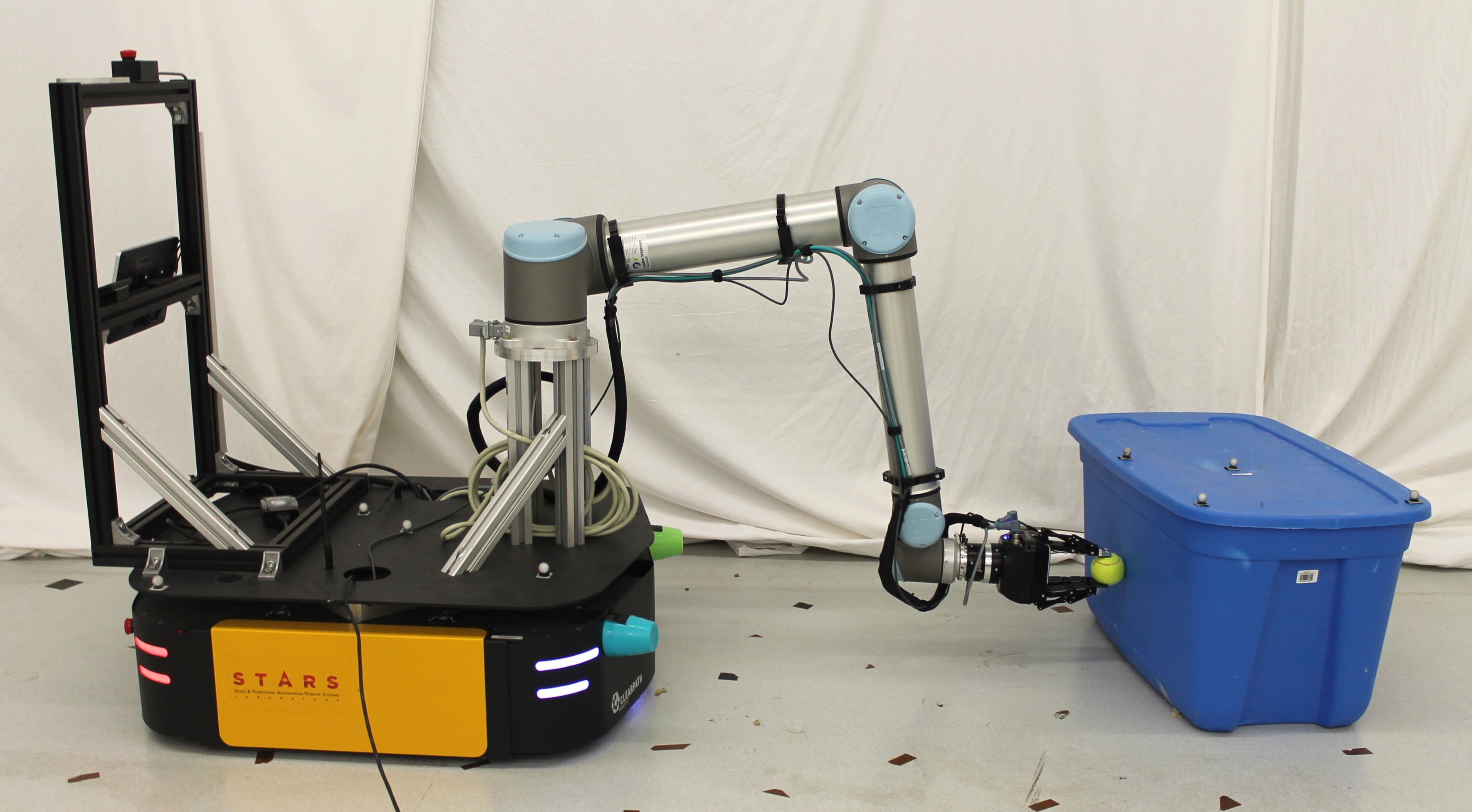
Figure 1: Our robot pushing a blue box across the floor using single-point contact. The contact force is measured by a force-torque sensor in the robot’s wrist, but no other measurements of the object are provided.

The main contribution of this work is to present the first controller for pushing objects with single-point contact based only on force feedback. We show that it successfully pushes objects along a desired straight-line path with single-point contact. We demonstrate the robustness of the controller by simulating pushes using a wide variety of slider parameters and initial states. We also present real hardware experiments in which a mobile manipulator successfully pushes different objects across a room (see Fig. 1). Notably, we do not assume that sufficient friction is available to prevent slip at the contact point. Indeed, we will see that slipping is a natural part of the behaviour of our controller and does not necessarily lead to task failure.

We first briefly described a preliminary version of this controller in [1]. In the current work we refine the control law, add a term to track a desired line, provide an analysis of its robustness in simulation, and perform more numerous and challenging real-world experiments.

II Related Work

Research on robotic pushing began with Mason [2]. The approaches that followed were typically either open-loop planning methods that rely on multi-point contact with a fence for stability [3, 4] or feedback-based approaches based on vision [5, 6] or tactile sensing [7, 8]. Tactile sensing is the most similar to our work, though we assume only a single contact force vector is available, rather than the contact angle and normal that a tactile sensor provides.

An FT sensor is used with a fence to orient polygonal parts using a sequence of one-dimensional pushes in [9], which was shown to require less pushes than the best sensorless alternative [10]. Another use of an FT sensor was in [11], where FT measurements are used to detect slip while pushing. In constrast, we do not detect slip; rather, our closed-loop dynamics are stable despite (unmeasured) slip.

More recent work has turned to learned-based approaches to model the complicated pushing dynamics arising from uncertain friction distributions and object parameters [12, 13]. Another line of work [14, 15] uses model predictive control (MPC) for fast online replanning. These methods are powerful but typically assume at least visual feedback is available (to localize the slider) and require either considerable training data for learning or an existing model of the slider. A survey on robotic pushing can be found in [16]. None of these methods are based only on force feedback.

III Methodology

We first describe the model of the slider used for simulation and then present our controller for pushing the slider based on force feedback.

III-A Model of Quasistatic Pushing

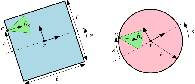
Figure 2: Examples of a square and a circular slider, located at position $\bm{r}$ and orientation $\phi$ in the global frame. The contact with the pusher is located at point $\bm{c}$, which is distance $s$ along the slider’s edge. The contact force must lie in the friction cone at the contact point (shown in green).

We use a model of quasistatic planar pushing equivalent to that presented in [8], which we briefly review here. Let $\bm{p}=[f_{x},f_{y},\tau]^{T}$ be the generalized force acting on the slider, where $(f_{x},f_{y})$ is the force and $\tau$ is the torque. Under the ellipsoidal limit surface model, this force must lie within the ellipsoid defined by

$$\bm{p}^{T}\bm{M}\bm{p}\leq 1,$$ (1)

where $\bm{M}=\operatorname{\mathrm{diag}}(f_{\max}^{-2},f_{\max}^{-2},\tau_{\max}^{-2})$ represents the maximum frictional load between the slider and the support plane (i.e., the ground). When the object is moving, (1) holds with equality. For simplicity we will assume uniform support friction, which means that the center of friction corresponds to the slider’s CoM projected onto the support plane. If we assume that the slider’s pressure distribution is concentrated at a particular distance $d$ from the CoM, then $\tau_{\max}=d\cdot f_{\max}$. When the pressure distribution is uniform, then $d=(\int_{A}\|\bm{a}\|dA)/(\int_{A}dA)$, where $A$ is the support area, $dA$ is a differential element of area of $A$, and $\bm{a}$ is the position of $dA$.

The system state is $\bm{x}=[x,y,\phi,s]^{T}$, where $\bm{r}=[x,y]^{T}$ is the slider’s position, $\phi$ is its orientation, and $s$ is the distance of the contact point $\bm{c}$ along the slider’s edge (see Fig. 2). The slider’s generalized velocity about the CoM and expressed in the body frame is $\bm{\varpi}=[v_{x},v_{y},\omega]^{T}$, with linear velocity $(v_{x},v_{y})$ and angular velocity $\omega$. Under quasistatic pushing, $\bm{\varpi}$ is in the direction normal to the boundary of (1). Let $\bm{v}_{o}\in\mathbb{R}^{2}$ be the slider’s velocity at the contact point and $\bm{v}_{p}\in\mathbb{R}^{2}$ be the pusher’s velocity; these are equal if the contact is sticking, but the magnitude of $\bm{v}_{p}$ is larger during slipping. We have the relationship $\bm{v}_{o}=\bm{W}_{c}^{T}\bm{\varpi}$, where

$$\bm{W}_{c}^{T}=\begin{bmatrix}1&0&-y_{c}\\ 0&1&x_{c}\end{bmatrix},$$

for contact point $\bm{c}=[x_{c},y_{c}]^{T}$ expressed in the body frame.

We can conveniently express the slider’s equations of motion as the solution to the quadratic program

$$\min_{\bm{\varpi},\alpha,\bm{\eta}} \quad\alpha^{2}$$ (2)

subject to $$\quad\bm{\varpi}=\bm{M}\bm{W}_{c}\bm{\eta}$$

$$\quad\bm{v}_{p}=\bm{W}_{c}^{T}\bm{\varpi}+\alpha\hat{\bm{n}}_{c}^{\perp}$$

$$\quad\bm{\eta}\in\mathcal{FC},$$

where $\alpha$ is the contact’s velocity along the current edge of the slider (i.e., the slip velocity), $\bm{\eta}$ is a vector parallel to the contact force, $\hat{\bm{n}}_{c}^{\perp}$ is a unit vector perpendicular to the contact normal, and $\mathcal{FC}=\{\bm{f}\in\mathbb{R}^{2}\mid|\hat{\bm{n}}_{c}^{\perp}\cdot\bm{f}|\leq\mu_{c}\hat{\bm{n}}_{c}\cdot\bm{f}\}$ is the friction cone at the contact with friction coefficient $\mu_{c}$. If desired, we can obtain the actual contact force $\bm{f}$ by substituting $\bm{p}=\bm{W}_{c}\bm{\eta}$ into the boundary of the limit surface (1) to obtain

$$\bm{f}=(\bm{\eta}^{T}\bm{W}_{c}^{T}\bm{M}\bm{W}_{c}\bm{\eta})^{-1/2}\bm{\eta}.$$

Intuitively, (2) tries to find the object velocity $\bm{\varpi}$ which corresponds to a feasible contact force and produces as little slip as possible. The system’s contact modes (sticking, sliding left, sliding right) correspond to particular sets of active constraints of (2). The pusher’s contact velocity $\bm{v}_{p}$ is given as the input to the system. If $\bm{v}_{p}$ is pulling away from the object (i.e., $\hat{\bm{n}}_{c}\cdot\bm{v}_{p}<0$), then (2) is infeasible. Assuming the pusher and slider maintain contact, we can simulate the entire system forward in time by integrating $\bm{\varpi}$ and $\alpha$. The formulation (2) produces the same results as the analytical equations in [8], but the correspondence between contact modes and active constraints may aid the intuition.

III-B Pushing Controller

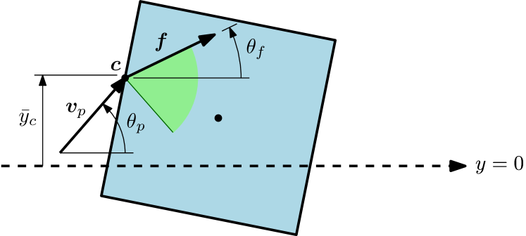
Figure 3: Example of our the pushing controller. The goal is to push the box along the line $y=0$ by pushing with velocity $\bm{v}_{p}$ at the contact point $\bm{c}$. The pushing angle $\theta_{p}$ is proportional to the lateral offset $\bar{y}_{c}$ and measured force angle $\theta_{f}$. In this example, the commanded $\bm{v}_{p}$ will eventually rotate the object so that the contact force points back toward the desired path along $y=0$. Depending on the contact friction coefficient $\mu_{c}$, the contact point is free to slip along the object’s edge over the course of a trajectory.

We now turn our attention to generating the pusher velocity $\bm{v}_{p}$ given measurements of the contact force $\bm{f}$. Let $\bar{\bm{v}}_{p}$ and ${\bar{\bm{f}\mkern 5.0mu}\mkern-5.0mu}{}$ be these same quantities but expressed in the global frame; indeed, since we do not assume to know the orientation of the slider, we cannot work in the local frame. Let us express these quantities in polar form as

$$\bar{\bm{v}}_{p} =\|\bar{\bm{v}}_{p}\|\cdot\begin{bmatrix}\cos\theta_{p}\\ \sin\theta_{p}\end{bmatrix}, {\bar{\bm{f}\mkern 5.0mu}\mkern-5.0mu}{} =\|{\bar{\bm{f}\mkern 5.0mu}\mkern-5.0mu}{}\|\cdot\begin{bmatrix}\cos\theta_{f}\\ \sin\theta_{f}\end{bmatrix}.$$

We set the pushing speed $\|\bar{\bm{v}}_{p}\|$ constant but control the pushing angle $\theta_{p}$. Our goal is to track a given straight-line path, which we will assume without loss of generality to be along the $x$-axis of the global frame (i.e., the line $y=0$ with $x$ increasing). Given an approximate initial position of the slider, we assume that the robot can be positioned so that it starts in contact with the slider and is approximately aligned with the desired pushing direction. Our control law is simply

$$\theta_{p}=(k_{f}+1)\theta_{f}+k_{y}\bar{y}_{c},$$ (3)

where $k_{f},k_{y}>0$ are tunable gains and $\bar{y}_{c}$ is the lateral deviation of the contact point from the desired path (see Fig. 3). The first term steers toward a stable pushing direction and the second term steers toward the desired path. Ultimately, the controller converges to a configuration where the contact force lies along the desired path. Notice that the controller does not depend explicitly on any slider parameters, and can thus be used to push a variety of unknown objects. In particular, we do not require knowledge of the support friction, pressure distribution, or contact friction, which are often uncertain and subject to change. Depending on the contact friction coefficient $\mu_{c}$, the contact point may slip or stick along the edge of the object over the course of a successful push, which is not a problem for our controller.

IV Simulations

We first validate our controller in simulation with a square and circular slider, as shown in Fig. 2, using the equations of motion (2) and our control law (3). The square has side length $\ell=$1\text{\,}\mathrm{m}$$ and the circle has radius $\rho=$0.5\text{\,}\mathrm{m}$$; the CoMs are located at the centroids. For each slider, we assess the robustness of our controller by running simulations with different combinations of initial state $\bm{x}_{0}=[0,y_{0},\phi_{0},s_{0}]^{T}$, contact friction, and pressure distribution (encoded in $\tau_{\max}$), as listed in Table I. We use pusher speed $\|\bar{\bm{v}}_{p}\|=$0.1\text{\,}\mathrm{m}\mathrm{/}\mathrm{s}$$, controller gains $k_{f}=0.1$ and $k_{y}=0.01$, and $f_{\max}=$1\text{\,}\mathrm{N}$$. The simulation timestep is $10\text{\,}\mathrm{m}\mathrm{s}$.

Table I: Initial states and parameters used for simulation of the square and circular sliders. Every combination of states and parameters is used, for a total of $3^{5}=243$ combinations per slider. The values of $\tau_{\max}$ depend on the slider shape, with $\bar{\tau}$ computed assuming a uniform pressure distribution and $\hat{\tau}$ computed assuming the pressure is concentrated at maximum distance from the CoM.

Parameter	Symbol	Values	Unit
Initial lateral offset	$y_{0}$	$-40$, $0$, $40$	$\mathrm{c}\mathrm{m}$
Initial contact offset	$s_{0}$	$-40$, $0$, $40$	$\mathrm{c}\mathrm{m}$
Initial orientation	$\phi_{0}$	$-\pi/8$, $0$, $\pi/8$	$\mathrm{r}\mathrm{a}\mathrm{d}$
Contact friction	$\mu_{c}$	$0$, $0.5$, $1.0$	$-$
Max. torsional load	$\tau_{\max}$	$0.1\bar{\tau}$, $\bar{\tau}$, $\hat{\tau}$	$\mathrm{N}\mathrm{m}$

The position trajectories for each of the $3^{5}=243$ parameter combinations per slider are shown in Fig. 4. Our controller successfully steers both sliders to the desired path along the positive $x$-axis for every parameter combination with the same controller gains. While $k_{y}$ could be increased to reduce the deviation from the desired path, we found that a larger $k_{y}$ was not stable for all of these parameter combinations.

Four sample trajectories are shown in Fig. 5. In particular, notice the difference between the two trajectories of the square slider. The first has zero contact friction ($\mu_{c}=0$), and we see that the contact point quickly slips toward the center of the square’s edge. In contrast, the second trajectory has high contact friction ($\mu_{c}=1$): the contact point does not slip and a stable push is achieved with a large angle between the contact normal and pushing direction.

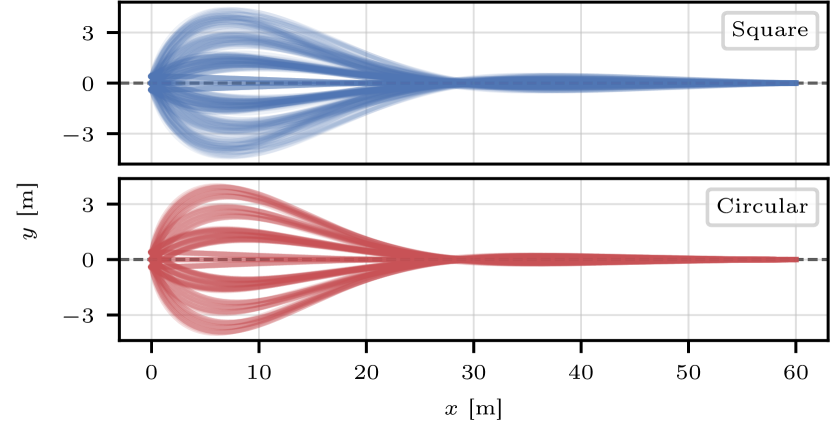
Figure 4: Simulated trajectories for all $243$ combinations of parameters given in Table I for the square and circular sliders shown in Fig. 2. Each trajectory has a duration of $10\text{\,}\mathrm{m}\mathrm{i}\mathrm{n}$. All trajectories converge to the desired path $y=0$ using our control law with the same set of gains $k_{f}=0.1$ and $k_{y}=0.01$.

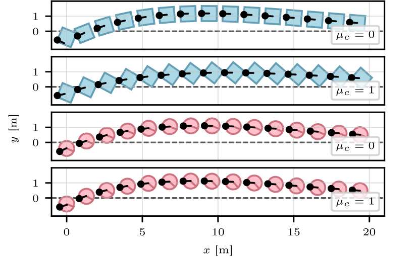
Figure 5: Samples of simulated trajectories with initial state $(x_{0},y_{0},s_{0},\phi_{0})=(0,$-40\text{\,}\mathrm{c}\mathrm{m}$,$-40\text{\,}\mathrm{c}\mathrm{m}$,-\pi/8)$ and a uniform pressure distribution. Results are shown for each slider with low and high contact friction. Contact point and pushing direction are shown in black. The orientation of the circular slider is indicated by the red line between its center and edge, which is aligned with the body frame’s $x$-axis.

V Hardware Experiments

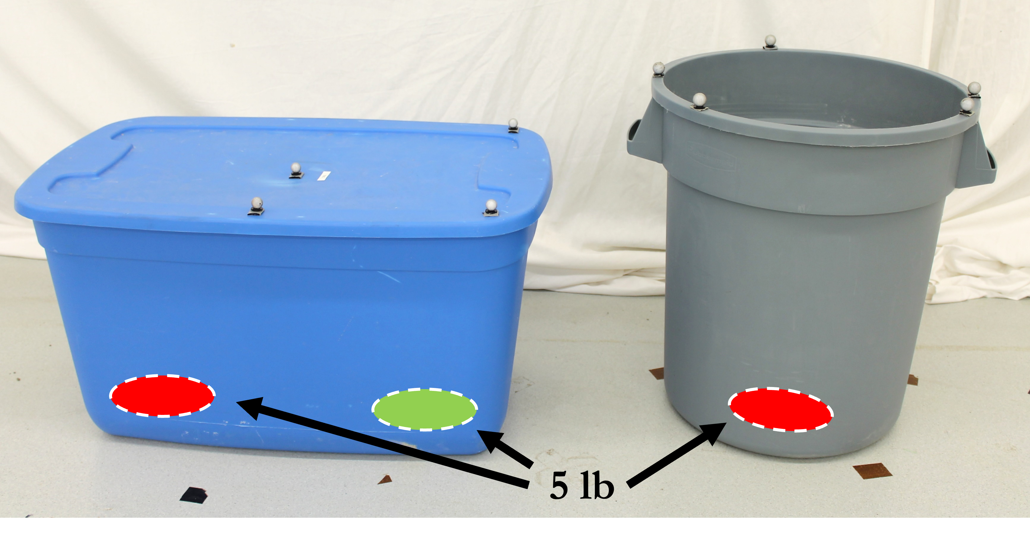
Figure 6: The “box” and “barrel” sliders used for real-world experiments. Each is empty except for $5\text{\,}\mathrm{l}\mathrm{b}$ weights located approximately at the colored circles. The red weights are always present, but we add or remove the green weight to vary the mass and pressure distribution of the box. Motion capture is used to record the sliders’ trajectories, but is not used for control.

We now demonstrate our controller in real-world experiments. The robot used for pushing is a mobile manipulator consisting of a UR10 arm mounted on a Ridgeback omnidirectional base (see Fig. 1). The arm’s wrist is equipped with a Robotiq FT 300 force-torque sensor. Since we are only concerned with pushing in the $x$-$y$ plane, we fix the joint angles of the arm and the orientation of the base and only control the linear velocity of the base by commanding $\bar{\bm{v}}_{p}$. The base is localized using a Vicon motion capture system, which is also used to record the trajectories of the sliders.

We test our controller’s ability to push a box and a barrel (shown in Fig. 6) across the floor, each of which contains $5\text{\,}\mathrm{l}\mathrm{b}$ weights. We vary the amount of weight (either $5$ or $10\text{\,}\mathrm{l}\mathrm{b}$) in the box to provide additional variety in the slider mass and pressure distribution. We assume that the height of the contact point is such that the sliders do not tip over.

We continue to use $\|\bar{\bm{v}}_{p}\|=$0.1\text{\,}\mathrm{m}\mathrm{/}\mathrm{s}$$ and $k_{f}=0.1$, but we increase $k_{y}$ to $0.3$. A lower value of $k_{y}$ was required in simulation so that the controller was stable for all combinations of parameters, but for these real-world experiments we found that a higher $k_{y}$ is more effective for tracking the desired path $y=0$. In general, the controller gains can be tuned to give better tracking performance when the set of possible slider parameters is smaller.

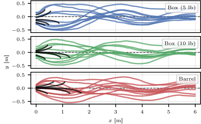
Figure 7: Position trajectories for real sliders pushed starting from various lateral offsets. Ten trajectories using our pushing control law are shown for each slider (in color). We compare against an open-loop controller, which just commands the robot to move forward with constant speed $\|\bar{\bm{v}}_{p}\|$. Five open-loop trajectories are shown for each slider (in black). The open-loop trajectories end once contact between the pusher and slider is lost. All open-loop trajectories fail within $2\text{\,}\mathrm{m}$, whereas our controller is able to push the objects across the full length of the room.

The experimental results are shown in Fig. 7. Ten trajectories using our pushing control law are shown for each slider. We compare against an open-loop controller, which just commands the robot to move forward with constant speed $\|\bar{\bm{v}}_{p}\|$. Five open-loop trajectories are shown for each slider. Open-loop pushing with single-point contact is unstable, and indeed we see that the open-loop trajectories quickly fail. In contrast, our closed-loop pushing controller successfully pushes the sliders across the full $6\text{\,}\mathrm{m}$ length of the room.

It should be noted that the trajectories do not converge perfectly to the desired path $y=0$, at least not within the available $6\text{\,}\mathrm{m}$ distance. This is expected in the real world, as the slider is constantly perturbed by imperfections on the surface of the ground as it slides, which must then be corrected by the controller. Indeed, as can be partially seen in Fig.1, the floor of the room has various pieces of tape and other markings which change the surface friction properties as the object slides. Regardless, in Fig. 7 we see that the controller keeps the slider within a corridor of approximately $1\text{\,}\mathrm{m}$ width around $y=0$, even with considerable initial lateral offsets between pusher and slider.

VI Conclusion

We presented a control law for quasistatic robotic planar pushing with single-point contact using only force feedback, which does not require known slider parameters or pose feedback, and we demonstrated its robustness in simulated and real-world experiments. Subsequent work will further investigate the theoretical properties of the controller and apply it to more challenging environments, such as those with obstacles.

References

- [1] A. Heins, M. Jakob, and A. P. Schoellig, “Mobile manipulation in unknown environments with differential inverse kinematics control,” in Proc. Conf. on Robots and Vision, 2021, pp. 64–71.
- [2] M. T. Mason, “Mechanics and planning of manipulator pushing operations,” Int. J. of Robotics Research, vol. 5, no. 3, pp. 53–71, 1986.
- [3] K. M. Lynch and M. T. Mason, “Stable pushing: Mechanics, controllability, and planning,” Int. J. of Robotics Research, vol. 15, no. 6, pp. 533–556, 1996.
- [4] S. Akella and M. T. Mason, “Posing polygonal objects in the plane by pushing,” Int. J. of Robotics Research, vol. 17, no. 1, pp. 70–88, 1998.
- [5] R. Emery and T. Balch, “Behavior-based control of a non-holonomic robot in pushing tasks,” in Proc. IEEE Int. Conf. on Robotics and Automation, vol. 3, 2001, pp. 2381–2388.
- [6] T. Igarashi, Y. Kamiyama, and M. Inami, “A dipole field for object delivery by pushing on a flat surface,” in Proc. IEEE Int. Conf. on Robotics and Automation, 2010, pp. 5114–5119.
- [7] Y. Okawa and K. Yokoyama, “Control of a mobile robot for the push-a-box operation,” in Proc. IEEE Int. Conf. on Robotics and Automation, 1992, pp. 761–766.
- [8] K. M. Lynch, H. Maekawa, and K. Tanie, “Manipulation and active sensing by pushing using tactile feedback,” in Proc. IEEE/RSJ Int. Conf. on Intelligent Robots and Systems, 1992, pp. 416–421.
- [9] S. Rusaw, K. Gupta, and S. Payandeh, “Part orienting with a force/torque sensor,” in Proc. IEEE Int. Conf. on Robotics and Automation, 1999, pp. 2545–2550.
- [10] S. Akella, W. H. Huang, K. M. Lynch, and M. T. Mason, “Parts feeding on a conveyor with a one joint robot,” Algorithmica, vol. 26, no. 3, pp. 313–344, 2000.
- [11] F. Ruiz-Ugalde, G. Cheng, and M. Beetz, “Fast adaptation for effect-aware pushing,” in Proc. IEEE-RAS Int. Conf. on Humanoid Robots, 2011, pp. 614–621.
- [12] M. Bauza, F. R. Hogan, and A. Rodriguez, “A data-efficient approach to precise and controlled pushing,” in Proc. Conf. on Robot Learning, 2018, pp. 336–345.
- [13] J. Li, W. S. Lee, and D. Hsu, “Push-net: Deep planar pushing for objects with unknown physical properties,” in Proc. Robotics: Science and Systems, 2018.
- [14] F. R. Hogan and A. Rodriguez, “Feedback control of the pusher-slider system: A story of hybrid and underactuated contact dynamics,” in Proc. Algorithmic Foundations of Robotics, 2020, pp. 800–815.
- [15] W. C. Agboh and M. R. Dogar, “Pushing fast and slow: Task-adaptive planning for non-prehensile manipulation under uncertainty,” in Proc. Algorithmic Foundations of Robotics, 2020, pp. 160–176.
- [16] J. Stüber, C. Zito, and R. Stolkin, “Let’s push things forward: A survey on robot pushing,” Frontiers in Robotics and AI, vol. 7, 2020.