Difference of Submodular Minimization via DC Programming

Abstract

Minimizing the difference of two submodular (DS) functions is a problem that naturally occurs in various machine learning problems. Although it is well known that a DS problem can be equivalently formulated as the minimization of the difference of two convex (DC) functions, existing algorithms do not fully exploit this connection. A classical algorithm for DC problems is called the DC algorithm (DCA). We introduce variants of DCA and its complete form (CDCA) that we apply to the DC program corresponding to DS minimization. We extend existing convergence properties of DCA, and connect them to convergence properties on the DS problem. Our results on DCA match the theoretical guarantees satisfied by existing DS algorithms, while providing a more complete characterization of convergence properties. In the case of CDCA, we obtain a stronger local minimality guarantee. Our numerical results show that our proposed algorithms outperform existing baselines on two applications: speech corpus selection and feature selection.

1 Introduction

We study the difference of submodular (DS) functions minimization problem

$$\min_{X\subseteq V}F(X):=G(X)-H(X),$$ (1)

where $G$ and $H$ are normalized submodular functions (see Section 2 for definitions). We denote the minimum of (1) by $F^{\star}$. Submodular functions are set functions that satisfy a diminishing returns property, which naturally occurs in a variety of machine learning applications. Many of these applications involve DS minimization, such as feature selection, probabilistic inference (Iyer & Bilmes, 2012), learning discriminatively structured graphical models (Narasimhan & Bilmes, 2005), and learning decision rule sets (Yang et al., 2021). In fact, this problem is ubiquitous as any set function can be expressed as a DS function, though finding a DS decomposition has exponential complexity in general (Narasimhan & Bilmes, 2005; Iyer & Bilmes, 2012).

Unlike submodular functions which can be minimized in polynomial time, minimizing DS functions up to any constant factor multiplicative approximation requires exponential time, and obtaining any positive polynomial time computable multiplicative approximation is NP-Hard (Iyer & Bilmes, 2012, Theorems 5.1 and 5.2). Even finding a local minimum (see Definition 2.1) of DS functions is PLS complete (Iyer & Bilmes, 2012, Section 5.3).

DS minimization was first studied in (Narasimhan & Bilmes, 2005), who proposed the submodular-supermodular (SubSup) procedure; an algorithm inspired by the convex-concave procedure (Yuille & Rangarajan, 2001), which monotonically reduces the objective function at every step and converges to a local minimum. Iyer & Bilmes (2012) extended the work of (Narasimhan & Bilmes, 2005) by proposing two other algorithms, the supermodular-submodular (SupSub) and the modular-modular (ModMod) procedures, which have lower per-iteration cost than the SubSup method, while satisfying the same theoretical guarantees.

The DS problem can be equivalently formulated as a difference of convex (DC) functions minimization problem (see Section 2). DC programs are well studied problems for which a classical popular algorithm is the DC algorithm (DCA) (Pham Dinh & Le Thi, 1997; Pham Dinh & Souad, 1988). DCA has been successfully applied to a wide range of non-convex optimization problems, and several algorithms can be viewed as special cases of it, such as the convex-concave procedure, the expectation-maximization (Dempster et al., 1977), and the iterative shrinkage-thresholding algorithm (Chambolle et al., 1998); see (Le Thi & Pham Dinh, 2018) for an extensive survey on DCA.

Existing DS algorithms, while inspired by DCA, do not fully exploit this connection to DC programming. In this paper, we apply DCA and its complete form (CDCA) to the DC program equivalent to the DS problem. We establish new connections between the two problems which allow us to leverage convergence properties of DCA to obtain theoretical guarantees on the DS problem that match ones by existing methods, and stronger ones when using CDCA. In particular, our key contributions are:

• We show that a special instance of DCA and CDCA, where iterates are integral, monotonically decreases the DS function value at every iteration, and converges with rate $O(1/k)$ to a local minimum and strong local minimum (see Definition 2.1) of the DS problem, respectively. DCA reduces to SubSup in this case.

• We introduce variants of DCA and CDCA, where iterates are rounded at each iteration, which allow us to add regularization. We extend the convergence properties of DCA and CDCA to these variants.

• CDCA requires solving a concave minimization subproblem at each iteration. We show how to efficiently obtain an approximate stationary point of this subproblem using the Frank-Wolfe (FW) algorithm.

• We study the effect of adding regularization both theoretically and empirically.

• We demonstrate that our proposed methods outperform existing baselines empirically on two applications: speech corpus selection and feature selection.

1.1 Additional related work

An accelerated variant of DCA (ADCA) which incorporates Nesterov’s acceleration into DCA was presented in (Nhat et al., 2018). We investigate the effect of acceleration in our experiments (Section 5). Kawahara & Washio (2011) proposed an exact branch-and-bound algorithm for DS minimization, which has exponential time-complexity. Maehara & Murota (2015) proposed a discrete analogue of the continuous DCA for minimizing the difference of discrete convex functions, of which DS minimization is a special case, where the proposed algorithm reduces to SubSup. Several works studied a special case of the DS problem where $G$ is modular (Sviridenko et al., 2017; Feldman, 2019; Harshaw et al., 2019), or approximately modular (Perrault et al., 2021), providing approximation guarantees based on greedy algorithms. El Halabi & Jegelka (2020) provided approximation guarantees to the related problem of minimizing the difference between an approximately submodular function and an approximately supermodular function. In this work we focus on general DS minimization, we discuss some implications of our results to certain special cases in Appendix H.

2 Preliminaries

We begin by introducing our notation and relevant background on DS and DC minimization.

Notation:

Given a ground set $V=\{1,\cdots,d\}$ and a set function $F:2^{V}\to\mathbb{R}$, we denote the marginal gain of adding an element $i$ to a set $X\subseteq V$ by $F(i|X)=F(X\cup\{i\})-F(X)$. The indicator vector $\mathds{1}_{X}\in\mathbb{R}^{d}$ is the vector whose $i$-th entry is $1$ if $i\in X$ and $0$ otherwise. Let $S_{d}$ denote the set of permutations on $V$. Given $\sigma\in S_{d}$, set $S^{\sigma}_{k}:=\{\sigma(1),\cdots,\sigma(k)\}$, with $S^{\sigma}_{0}=\emptyset$. The symmetric difference of two sets $X,Y$ is denoted by $X\Delta Y=(X\setminus Y)\cup(Y\setminus X)$. Denote by $\Gamma_{0}$ the set of all proper lower semicontinuous convex functions on $\mathbb{R}^{d}$. We write $\overline{\mathbb{R}}$ for $\mathbb{R}\cup\{+\infty\}$. Given a set $C\subseteq\mathbb{R}^{d},\delta_{C}$ denotes the indicator function of $C$ taking value $0$ on $C$ and $+\infty$ outside it. Throughout, $\|\cdot\|$ denotes the $\ell_{2}$-norm.

DS minimization

A set function $F$ is normalized if $F(\emptyset)=0$ and non-decreasing if $F(X)\leq F(Y)$ for all $X\subseteq Y$. $F$ is submodular if it has diminishing marginal gains: $F(i\mid X)\geq F(i\mid Y)$ for all $X\subseteq Y$, $i\in V\setminus Y$, supermodular if $-F$ is submodular, and modular if it is both submodular and supermodular. Given a vector $x\in\mathbb{R}^{d}$, $x$ defines a modular set function as $x(A)=\sum_{i\in A}x_{i}$. Note that minimizing the difference between two submodular functions is equivalent to maximizing the difference between two submodular functions, and minimizing or maximizing the difference of two supermodular functions.

Given the inapproximability of Problem (1), we are interested in obtaining approximate local minimizers.

Definition 2.1.

Given $\epsilon\geq 0$, a set $X\subseteq V$ is an $\epsilon$-local minimum of $F$ if $F(X)\leq F(X\cup i)+\epsilon\text{ for all }i\in V\setminus X$ and $F(X)\leq F(X\setminus i)+\epsilon\text{ for all }i\in X$. Moreover, $X$ is an $\epsilon$-strong local minimum of $F$ if $F(X)\leq F(Y)+\epsilon\text{ for all }Y\subseteq X\text{ and all }Y\supseteq X$.

In Appendix H, we show that if $F$ is submodular then any $\epsilon$-strong local minimum $\hat{X}$ of $F$ is also an $\epsilon$-global minimum, i.e., $F(\hat{X})\leq F^{\star}+\epsilon$. It was also shown in (Feige et al., 2011, Theorem 3.4) that if $F$ is supermodular then any $\epsilon$-strong local minimum $\hat{X}$ satisfies $\min\{F(\hat{X}),F(V\setminus\hat{X})\}\leq\tfrac{1}{3}F^{\star}+\tfrac{2}{3}\epsilon$. We further show relaxed versions of these properties for approximately submodular and supermodular functions in Appendix H. Moreover, the two notions of approximate local minimality are similar if $F$ is supermodular: any $\epsilon$-local minimum of $F$ is also an $\epsilon d$-strong local minimum of $F$ (Feige et al., 2011, Lemma 3.3). However, in general, a local miniumum can have an arbitrarily worse objective value than any strong local minimum, as illustrated in Example G.2.

Minimizing a set function $F$ is equivalent to minimizing a continuous extension of $F$ called the Lovász extension (Lovász, 1983) on the hypercube $[0,1]^{d}$ .

Definition 2.2 (Lovász extension).

Given a normalized set function $F$, its Lovász extension $f_{L}:\mathbb{R}^{d}\to\mathbb{R}$ is defined as follows: Given $x\in\mathbb{R}^{d}$ and $\sigma\in S_{d}$, with $x_{\sigma(1)}\geq\cdots\geq x_{\sigma(d)}$, $f_{L}(x):=\sum_{k=1}^{d}x_{\sigma(k)}F(\sigma(k)\mid S^{\sigma}_{k-1}).$

We make use of the following well known properties of the Lovász extension; see e.g. (Bach, 2013) and (Jegelka & Bilmes, 2011, Lemma 1) for item g.

Proposition 2.3.

For a normalized set function $F$, we have:

1. For all $X\subseteq V,F(X)=f_{L}(\mathds{1}_{X})$.

2. If $F=G-H$, then $f_{L}=g_{L}-h_{L}$.

3. $\min_{X\subseteq V}F(X)=\min_{x\in[0,1]^{d}}f_{L}(x)$.

4. Rounding: Given $x\in[0,1]^{d},\sigma\in S_{d}$ such that $x_{\sigma(1)}\geq\dots\geq x_{\sigma(d)}$, let $\hat{k}\in\mathop{{\rm argmin}}_{k=0,1,\dots,d}F(S^{\sigma}_{k})$, then $F(S^{\sigma}_{\hat{k}})\leq f_{L}(x).$ We denote this operation by $S^{\sigma}_{\hat{k}}=\mathrm{Round}_{F}(x)$.

5. $f_{L}$ is convex if and only if $F$ is submodular.

6. Let $F$ be submodular and define its base polyhedron

   Greedy algorithm: Given $x\in\mathbb{R}^{d},\sigma\in S_{d}$ such that $x_{\sigma(1)}\geq\dots\geq x_{\sigma(d)}$, define $y_{\sigma(k)}=F(\sigma(k)\mid S^{\sigma}_{k-1}),$ then $y$ is a maximizer of $\max_{s\in B(F)}\langle x,\,s\rangle$, $f_{L}$ is the support function of $B(F)$, i.e., $f_{L}(x)=\max_{s\in B(F)}\langle x,\,s\rangle$, and $y$ is a subgradient of $f_{L}$ at $x$.

7. If $F$ is submodular, then $f_{L}$ is $\kappa$-Lipschitz, i.e., $|f_{L}(x)-f_{L}(y)|\leq\kappa\|x-y\|$ for all $x,y\in\mathbb{R}^{d}$, with $\kappa=3\max_{X\subseteq V}|F(X)|$. If $F$ is also non-decreasing, then $\kappa=F(V)$.

These properties imply that Problem (1) is equivalent to

$$\min_{x\in[0,1]^{d}}f_{L}(x)=g_{L}(x)-h_{L}(x),$$ (2)

with $g_{L},h_{L}\in\Gamma_{0}$. In paticular, if $X^{*}$ is a minimizer of (1), then $1_{X^{*}}$ is a minimizer of (2), and if $x^{*}$ is a minimizer of (2) then $\mathrm{Round}_{F}(x^{*})$ is a minimizer of (1).

DC programming

For a function $f:\mathbb{R}^{d}\to\overline{\mathbb{R}}$, its domain is defined as $\mathrm{dom}\,f=\left\{x\in\mathbb{R}^{d}\,\left|\;f(x)<+\infty\right.\right\}$, and its Fenchel conjugate as $f^{*}(y)=\sup_{y\in\mathbb{R}^{d}}\langle x,\,y\rangle-f(x)$. For $\rho\geq 0$, $f$ is $\rho$-strongly convex if $f-\tfrac{\rho}{2}\|\cdot\|^{2}$ is convex. We denote by $\rho(f)$ the supremum over such values. We say that $f$ is locally polyhedral convex if every point in its epigraph has a relative polyhedral neighbourhood (Durier, 1988). For a convex function $f,\epsilon\geq 0$ and $x^{0}\in\mathrm{dom}\,f$, the $\epsilon$-subdifferential of $f$ at $x^{0}$ is defined by $\partial_{\epsilon}f(x^{0})=\left\{y\in\mathbb{R}^{d}\,\left|\;f(x)\geq f(x^{0})+\langle y,\,x-x^{0}\rangle-\epsilon,\forall x\in\mathbb{R}^{d}\right.\right\},$ while $\partial f(x^{0})$ stands for the exact subdifferential ($\epsilon=0)$. We use the same notation to denote the $\epsilon$-superdifferential of a concave function $f$ at $x^{0}$, defined by $\partial_{\epsilon}f(x^{0})=\left\{y\in\mathbb{R}^{d}\,\left|\;f(x)\leq f(x^{0})+\langle y,\,x-x^{0}\rangle+\epsilon,\forall x\in\mathbb{R}^{d}\right.\right\}.$ We also define $\mathrm{dom}\,\partial_{\epsilon}f=\left\{x\in\mathbb{R}^{d}\,\left|\;\partial_{\epsilon}f(x)\not=\emptyset\right.\right\}$.

The $\epsilon$-subdifferential of a function $f\in\Gamma_{0}$ and its conjugate $f^{*}$ have the following relation (Urruty & Lemaréchal, 1993, Part II, Proposition 1.2.1).

Proposition 2.4.

For any $f\in\Gamma_{0},\epsilon\geq 0$, we have

$$y\in\partial_{\epsilon}f(x)\Leftrightarrow f^{*}(y)+f(x)-\langle y,\,x\rangle\leq\epsilon\Leftrightarrow x\in\partial_{\epsilon}f^{*}(y).$$

A general DC program takes the form

$$\min_{x\in\mathbb{R}^{d}}f(x):=g(x)-h(x)$$ (3)

where $g,h\in\Gamma_{0}$. We assume throughout the paper that the minimum of (3) is finite and denote it by $f^{\star}$. The DC dual of (3) is given by (Pham Dinh & Le Thi, 1997)

$$f^{*}=\min_{y\in\mathbb{R}^{d}}h^{*}(y)-g^{*}(y).$$ (4)

The main idea of DCA is to approximate $h$ at each iteration $k$ by its affine minorization $h(x^{k})+\langle y^{k},\,x-x^{k}\rangle$, with $y^{k}\in\partial h(x^{k})$, and minimize the resulting convex function. DCA can also be viewed as a primal-dual subgradient method. We give in Algorithm 1 an approximate version of DCA with inexact iterates. Note that $\partial g^{*}(y^{k})=\mathop{{\rm argmin}}_{x\in\mathbb{R}^{d}}g(x)-\langle y^{k},\,x\rangle$, and any $\epsilon$-solution $x^{k+1}$ to this problem will satisfy $x^{k+1}\in\partial_{\epsilon_{x}}g^{*}(y^{k})$, by Proposition 2.4.

Algorithm 1 Approximate DCA

1:  $\epsilon,\epsilon_{x},\epsilon_{y}\geq 0,x^{0}\in\mathrm{dom}\,\partial g$, $k\leftarrow 0$.

2:  while $f(x^{k})-f(x^{k+1})>\epsilon$ do

3:     $y^{k}\in\partial_{\epsilon_{y}}h(x^{k})$

4:     $x^{k+1}\in\partial_{\epsilon_{x}}g^{*}(y^{k})$

5:     $k\leftarrow k+1$

6:  end while

The following lemma, which follows from Proposition 2.4, provides a sufficient condition for DCA to be well defined, i.e, one can construct the sequences $\{x^{k}\}$ and $\{y^{k}\}$ from an arbitrary initial point $x^{0}\in\mathrm{dom}\,\partial g$.

Lemma 2.5.

DCA is well defined if

$$\mathrm{dom}\,\partial g\subseteq\mathrm{dom}\,\partial h\text{ and }\mathrm{dom}\,\partial h^{*}\subseteq\mathrm{dom}\,\partial g^{*}$$

Since Problem (3) is non-convex, we are interested in notions of approximate stationarity.

Definition 2.6.

For $\epsilon,\epsilon_{1},\epsilon_{2}\geq 0$, a point $x$ is an $(\epsilon_{1},\epsilon_{2})$-critical point of $g-h$ if $\partial_{\epsilon_{1}}g(x)\cap\partial_{\epsilon_{2}}h(x)\neq\emptyset$. Moreover, $x$ is an $\epsilon$-strong critical point if $\partial h(x)\subseteq\partial_{\epsilon}g(x)$.

Note that the two notions of criticality are equivalent when $h$ is differentiable and $\epsilon_{1}=\epsilon,\epsilon_{2}=0$. The following proposition provides necessary and sufficient conditions for approximate local optimality based on approximate criticality.

Proposition 2.7.

Let $g,h\in\Gamma_{0}$ and $\epsilon\geq 0$. Then we have:

1. Let $\hat{x},x$ be two points satisfying $\partial_{\epsilon_{1}}g(\hat{x})\cap\partial_{\epsilon_{2}}h(x)\not=\emptyset$, for some $\epsilon_{1},\epsilon_{2}\geq 0$ such that $\epsilon_{1}+\epsilon_{2}=\epsilon$, then $g(\hat{x})-h(\hat{x})\leq g(x)-h(x)+\epsilon$. Moreover, if $\hat{x}$ admits a neighbourhood $U$ such that $\partial_{\epsilon_{1}}g(\hat{x})\cap\partial_{\epsilon_{2}}h(x)\not=\emptyset$ for all $x\in U\cap\mathrm{dom}\,g$, then $\hat{x}$ is an $\epsilon$-local minimum of $g-h$. Conversely, if $\hat{x}$ is an $\epsilon$-local minimum of $g-h$, then it is also an $\epsilon$-strong critical point of $g-h$.

2. If $h$ is locally polyhedral convex, then $\hat{x}$ is an $\epsilon$-local minimum of $g-h$ if and only if it is an $\epsilon$-strong critical point of $g-h$.

Proof sketch.

This extends the conditions for $\epsilon=0$ in (Le Thi & Pham Dinh, 1997, Theorem 4 and Corollary 2) and (Hiriart-Urruty, 1989, Proposition 3.1) to $\epsilon\geq 0$. The proof is given in Section D.1. ∎

DCA converges in objective values, and in iterates if $g$ or $h$ is strongly convex, to a critical point (Pham Dinh & Le Thi, 1997, Theorem 3). We can always make the DC components strongly convex by adding $\tfrac{\rho}{2}\|\cdot\|^{2}$ to both $g$ and $h$. A special instance of DCA, called complete DCA, converges to a strong critical point, but requires solving concave minimization subproblems (Pham Dinh & Souad, 1988, Theorem 3). CDCA picks valid DCA iterates $y^{k},x^{k+1}$ that minimize the dual and primal DC objectives, respectively. We consider an approximate version of CDCA with the following iterates.

$$y^{k} \in\mathop{{\rm argmin}}\{h^{*}(y)-g^{*}(y):y\in\partial h(x^{k})\}$$

$$=\mathop{{\rm argmin}}\{\langle y,\,x^{k}\rangle-g^{*}(y):y\in\partial h(x^{k})\},$$ (5a)

$$x^{k+1} \in\mathop{{\rm argmin}}\{g(x)-h(x):x\in\partial_{\epsilon_{x}}g^{*}(y^{k})\}$$

$$=\mathop{{\rm argmin}}\{\langle x,\,y^{k}\rangle-h(x):x\in\partial_{\epsilon_{x}}g^{*}(y^{k})\}.$$ (5b)

3 DS Minimization via DCA

In this section, we apply DCA to the DC program (2) corresponding to DS minimization. We consider the DC decomposition $f=g-h$, where

$$g=g_{L}+\delta_{[0,1]^{d}}+\tfrac{\rho}{2}\|\cdot\|^{2}\text{ and }h=h_{L}+\tfrac{\rho}{2}\|\cdot\|^{2},$$ (6)

with $\rho\geq 0$. Starting from $x^{0}\in[0,1]^{d}$, the approximate DCA iterates (with $\epsilon_{y}=0$) are then given by

$$y^{k}\in\rho x^{k}+\partial h_{L}(x^{k}),$$ (7a)

$$x^{k+1}\text{ is an $\epsilon_{x}$-solution of }$$

$$\!\!\!\!\min_{x\in[0,1]^{d}}g_{L}(x)-\langle x,\,y^{k}\rangle+\tfrac{\rho}{2}\|x\|^{2}$$ (7b)

Note that the minimum $f^{*}=F^{*}$ of (2) is finite, since $f$ is finite. DCA is clearly well defined here; we discuss below how to obtain the iterates efficiently. One can also verify that the condition in Lemma 2.5 holds: $\mathrm{dom}\,\partial g=[0,1]^{d}\subseteq\mathrm{dom}\,\partial h=\mathbb{R}^{d}$ by Proposition 2.3-f, and $\mathrm{dom}\,\partial h^{*}=B(H)$ if $\rho=0$, $\mathbb{R}^{d}$ otherwise, hence in both cases $\mathrm{dom}\,\partial h^{*}\subseteq\mathrm{dom}\,\partial g^{*}=\mathbb{R}^{d}$, by Proposition 2.3-b,c.

Computational complexity

A subgradient of $h_{L}$ can be computed as described in Proposition 2.3-f in $O(d\log d+d~{}\text{EO}_{H})$ with $\text{EO}_{H}$ being the time needed to evaluate $H$ on any set. An $\epsilon_{x}$-solution of Problem (7b), for $\epsilon_{x}>0$, can be computed using the projected subgradient method (PGM) in $O(d\kappa^{2}/\epsilon_{x}^{2})$ iterations when $\rho=0$ and in $O(2(\kappa+\rho\sqrt{d})^{2}/\rho\epsilon_{x})$ when $\rho>0$ (Bubeck, 2014, Theorems 3.1 and 3.5), where $\kappa$ is the Lipschitz constant of $g_{L}(x)-\langle x,\,y^{k}\rangle$; see Proposition 2.3-g. The time per iteration of PGM is $O(d\log d+d~{}\text{EO}_{G})$.

When $\rho=0$, Problem (7b) is equivalent to a submodular minimization problem, since $\min_{x\in[0,1]^{d}}g_{L}(x)-\langle x,\,y^{k}\rangle=\min_{X\subseteq V}G(X)-y^{k}(X)$ by Proposition 2.3-b,c. Then we can take $x^{k+1}=\mathds{1}_{X^{k+1}}$ where $X^{k+1}\in\mathop{{\rm argmin}}_{X\subseteq V}G(X)-y^{k}(X)$. Several algorithms have been developed for minimizing a submodular function in polynomial time, exactly or within arbitrary accuracy $\epsilon_{x}>0$. Inexact algorithms are more efficient, with the current best runtime $\tilde{O}(d~{}\text{EO}_{G}/\epsilon_{x}^{2})$ achieved by (Axelrod et al., 2019). In this case, DCA reduces to the SubSup procedure of (Narasimhan & Bilmes, 2005) and thus satisfies the same theoretical guarantees; see Appendix A.

In what follows, we extend these guarantees to the general case where $x^{k}$ is not integral and $\rho\geq 0$, by leveraging convergence properties of DCA.

Theoretical guarantees

Existing convergence results of DCA in (Pham Dinh & Le Thi, 1997; Le Thi & Pham Dinh, 1997, 2005) consider exact iterates and exact convergence, i.e., $f(x^{k})=f(x^{k+1})$, which may require an exponential number of iterations, as shown in (Byrnes, 2015, Theorem 3.4) for SubSup. We extend these results to handle inexact iterates and approximate convergence.

Theorem 3.1.

Given any $f=g-h$, where $g,h\in\Gamma_{0}$, let $\{x^{k}\}$ and $\{y^{k}\}$ be generated by approximate DCA (Algorithm 1). Then for all $t_{x},t_{y}\in(0,1],k\in\mathbb{N}$, let $\bar{\rho}=\rho(g)(1-t_{x})+\rho(h)(1-t_{y})$ and $\bar{\epsilon}=\tfrac{\epsilon_{x}}{t_{x}}+\tfrac{\epsilon_{y}}{t_{y}}$, we have:

1. $\begin{aligned} f(x^{k})-f(x^{k+1})\geq\frac{\bar{\rho}}{2}\|x^{k}-x^{k+1}\|^{2}-\bar{\epsilon}\end{aligned}$.

2. For $\epsilon\geq 0$, if $f(x^{k})-f(x^{k+1})\leq\epsilon$, then $x^{k}$ is an $(\epsilon^{\prime},\epsilon_{y})$-critical point of $g-h$ with $y^{k}\in\partial_{\epsilon^{\prime}}g(x^{k})\cap\partial_{\epsilon_{y}}h(x^{k})$, $x^{k+1}$ is an $(\epsilon_{x},\epsilon^{\prime})$-critical point of $g-h$ with $y^{k}\in\partial_{\epsilon_{x}}g(x^{k+1})\cap\partial_{\epsilon^{\prime}}h(x^{k+1})$, where $\epsilon^{\prime}=\epsilon+\epsilon_{x}+\epsilon_{y}$, and $\frac{\bar{\rho}}{2}\|x^{k}-x^{k+1}\|^{2}\leq\bar{\epsilon}+\epsilon$.

3. $\begin{aligned} \min_{k\in\{0,1,\dots,K-1\}}f(x^{k})-f(x^{k+1})\leq\frac{f(x^{0})-f^{\star}}{K}.\end{aligned}$

4. If $\rho(g)+\rho(h)>0$, then

   $$\min_{k\in\{0,1,\dots,K-1\}}\|x^{k}-x^{k+1}\|\leq\sqrt{\frac{2}{\bar{\rho}}\big{(}\frac{f(x^{0})-f^{\star}}{K}+\bar{\epsilon}\big{)}}.$$

Proof sketch.

Items a and b with $\epsilon\!=\!\epsilon_{x}\!=\!\epsilon_{y}\!=\!0$ are proved in (Pham Dinh & Le Thi, 1997, Theorem 3). We extend them to $\epsilon,\epsilon_{x},\epsilon_{y}\!\geq\!0$ by leveraging properties of approximate subgradients. Item c is obtained by telescoping sum. ∎

Theorem 3.1 shows that approximate DCA decreases the objective $f$ almost monotonically (up to $\bar{\epsilon}$), and converges in objective values with rate $O(1/k)$, and in iterates with rate $O(1/\sqrt{k})$ if $\rho>0$, to an approximate critical point of $g-h$.

We present in Section E.1 a more detailed version of Theorem 3.1 and its full proof. In particular, we relate $f(x^{k})-f(x^{k+1})$ to a weaker measure of non-criticality, recovering the convergence rate provided in (Abbaszadehpeivasti et al., 2021, Corollary 4.1) on this measure. Approximate DCA with $\epsilon=0,\epsilon_{x}=\epsilon_{y}\geq 0$ was considered in (Vo, 2015, Theorem 1.4) showing that any limit points $\hat{x},\hat{y}$ of $\{x^{k}\},\{y^{k}\}$ satisfy $\hat{y}\in\partial_{3\epsilon_{x}}g(\hat{x})\cap\partial_{\epsilon_{x}}h(\hat{x})$ in this case. Our results are more general and tighter (at convergence $y^{K}\in\partial_{2\epsilon_{x}}g(x^{K})\cap\partial_{\epsilon_{x}}h(x^{K})$ in this case). For DS minimization, $y^{k}$ can be easily computed exactly ($\epsilon_{y}=0$). We consider $\epsilon_{y}>0$ to provide convergence results of FW on the concave subproblem required in CDCA (see Section 4).

The following corollary relates criticality on the DC problem (2) to local minimality on the DS problem (1).

Corollary 3.2.

Given $f=g-h$ as defined in (6), let $\{x^{k}\}$ and $\{y^{k}\}$ be generated by a variant of approximate DCA (7), where $x^{k}$ is integral, i.e., $x^{k}=\mathds{1}_{X^{k}}$ for some $X^{k}\subseteq V$, and $y^{k}-\rho x^{k}$ is computed as in Proposition 2.3-f. Then for all $k\in\mathbb{N},\epsilon\geq 0$, we have

1. If $f(x^{k})-f(x^{k+1})\leq\epsilon$, then

   $$F(X^{k})\leq F(S^{\sigma}_{\ell})+\epsilon^{\prime}\text{ for all $\ell\in V$},$$ (8)

   where

   $$\epsilon^{\prime}=\begin{cases}\sqrt{2\rho d(\epsilon+\epsilon_{x})}&\text{ if $\epsilon+\epsilon_{x}\leq\tfrac{\rho d}{2}$}\\ \tfrac{\rho d}{2}+\epsilon+\epsilon_{x}&\text{otherwise}.\end{cases}$$ (9)

   and $\sigma\in S_{d}$ is the permutation used to compute $y^{k}-\rho x^{k}$ in Proposition 2.3-f.

2. Given $d$ permutations $\sigma_{1},\cdots,\sigma_{d}\in S_{d}$, corresponding to decreasing orders of $x^{k}$ with different elements at $\sigma(|X^{k}|)$ or $\sigma(|X^{k}|+1)$, and the corresponding subgradients $y^{k}_{\sigma_{1}},\cdots,y^{k}_{\sigma_{d}}\in\partial h(x^{k})$ chosen as in Proposition 2.3-f, if we choose

   $$x^{k+1}=\mathop{{\rm argmin}}_{i\in V}\{f(x^{k+1}_{\sigma_{i}}):x^{k+1}_{\sigma_{i}}\in\partial_{\epsilon_{x}}g^{*}(y^{k}_{\sigma_{i}})\},$$

   then if $f(x^{k})-f(x^{k+1})\leq\epsilon$, Eq. 8 holds with $\sigma=\sigma_{i}$ for all $i\in V$. Hence, $X^{k}$ is an $\epsilon^{\prime}$-local minimum of $F$.

Proof sketch.

We observe that $y^{k}-\rho x^{k}\in\partial h_{L}(\mathds{1}_{S^{\sigma}_{\ell}})$ for all $\ell\in V$. Item a then follows from Theorem 3.1-b, Proposition 2.3-a,f, Proposition 2.7-a, and the relation between the $\epsilon$-subdifferentials of $g$ and $g-\frac{\rho}{2}\|\cdot\|^{2}$. Item b follows from Item a. See Section E.2. ∎

Theorem 3.1 and Corollary 3.2 show that DCA with integral iterates $x^{k}$ decreases the objective $F$ almost monotonically (up to $\bar{\epsilon}$), and converges to an $\epsilon^{\prime}$-local minimum of $F$ after at most $(f(x^{0})-f^{\star})/\epsilon$ iterations, if we consider $O(d)$ permutations for computing $y^{k}$. By a similar argument, we can further guarantee that the returned solution cannot be improved, by more than $\epsilon^{\prime}$, by adding or removing any $c$ elements, if we consider $O(d^{c})$ permutations for computing $y^{k}$.

Taking $\epsilon_{x}=0,\rho=0$ in Theorem 3.1 and Corollary 3.2, we recover all the theoretical properties of SubSup given in (Narasimhan & Bilmes, 2005; Iyer & Bilmes, 2012).

Effect of regularization

Theorem 3.1 shows that using a non-zero regularization parameter $\rho>0$ ensures convergence in iterates. Regularization also affects the complexity of solving Problem (7b); as discussed earlier $\rho>0$ leads to a faster convergence rate (except for very small $\rho$). On the other hand, Corollary 3.2 shows that for fixed $\epsilon$ and $\epsilon_{x}$, a larger $\rho$ may lead to a poorer solution. In practice, we observe that a larger $\rho$ leads to slower convergence in objective values $f(x^{k})$, but more accurate $x^{k}$ iterates, with $\rho>0$ always yielding the best performance with respect to $F$ (see Section C.1).

Note that when $\rho>0$ we can’t restrict $x^{k}$ to be integral, since the equivalence in Proposition 2.3-c does not hold in this case. It may also be advantageous to not restrict $x^{k}$ to be integral even when $\rho=0$, as we observe in our numerical results (Section C.3). A natural question arises here: can we still obtain an approximate local minimum of $F$ in this case? Given a fractional solution $x^{K}$ returned by DCA we can easily obtain a set solution with a smaller objective $F(X^{K})=f_{L}(\mathds{1}_{X^{K}})\leq f_{L}(x^{K})$ by rounding; $X^{K}=\mathrm{Round}_{F}(x^{K})$ as described in Proposition 2.3-d. However, rounding a fractional solution $x^{K}$ returned by DCA will not necessarily yield an approximate local minimum of $F$, even if $x^{K}$ is a local minimum of $f_{L}$, as we show in Example G.1. A simple workaround would be to explicitly check if the rounded solution is an $\epsilon^{\prime}$-local minimum of $F$. If not, we can restart the algorithm from $x^{K}=\mathds{1}_{\hat{X}^{K}}$ where $\hat{X}^{K}=\mathop{{\rm argmin}}_{|X\Delta X^{K}|=1}F(X)$, similarly to what was proposed in (Byrnes, 2015, Algorithm 1) for SubSup. This will guarantee that DCA converges to an $\epsilon^{\prime}$-local minimum of $F$ after at most $(f(x^{0})-f^{\star})/\epsilon$ iterations (see Proposition E.4). Such strategy is not feasible though if we want to guarantee convergence to an approximate strong local minimum of $F$, as we do in Section 4 with CDCA. We thus propose an alternative approach. We introduce a variant of DCA, which we call DCAR, where we round $x^{k}$ at each iteration.

DCA with rounding

Starting from $x^{0}\in\{0,1\}^{d}$, the approximate DCAR iterates are given by

$$y^{k},\tilde{x}^{k+1}\text{ as in \eqref{eq:DCASet-y} and \eqref{eq:DCASet-x} respectively,}$$ (10a)

$$x^{k+1}\leftarrow\mathds{1}_{X^{k+1}}\text{ where }X^{k+1}=\mathrm{Round}_{F}(\tilde{x}^{k+1}).$$ (10b)

Since $y^{k},\tilde{x}^{k+1}$ are standard approximate DCA iterates, then the properties in Theorem 3.1 apply to them, with $\epsilon_{y}=0$ and $x^{k+1}$ replaced by $\tilde{x}^{k+1}$. See Theorem E.5 for details. Since $x^{k}$ is integral in DCAR, Corollary 3.2 also holds. In particular, DCAR converges to an $\epsilon^{\prime}$-local minimum of $F$ after at most $(f(x^{0})-f^{\star})/\epsilon$ iterations, if we consider $O(d)$ permutations for computing $y^{k}$, with $\epsilon^{\prime}$ defined in (9).

4 DS Minimization via CDCA

As discussed in Section 2, CDCA is a special instance of DCA which is guaranteed to converge to a strong critical point. In this section, we apply CDCA to the DC program (2) corresponding to DS minimization, and show that the stronger guarantee on the DC program translates into a stronger guarantee on the DS problem. We use the same decomposition in (6).

Computational complexity

CDCA requires solving a concave minimization problem for each iterate update. The constraint polytope $\partial h(x^{k})=\rho x^{k}+\partial h_{L}(x^{k})$ in Problem (5a) can have a number of vertices growing exponentially with the number of equal entries in $x^{k}$. Thus, it is not possible to efficiently obtain a global solution of Problem (5a) in general. However, we can efficiently obtain an approximate critical point. Denote the objective

$$\phi_{k}(w)=\langle w,\,x^{k}\rangle-g^{*}(w).$$ (11)

We use an approximate version of the FW algorithm, which starting from $w^{0}\in\partial h(x^{k})$, has the following iterates:

$$s^{t} \in\partial_{\epsilon}\phi_{k}(w^{t})\supseteq x^{k}-\partial_{\epsilon}g^{*}(w^{t}),$$ (12a)

$$v^{t} \in\mathop{{\rm argmin}}\{\langle s^{t},\,w\rangle:w\in\partial h(x^{k})\},$$ (12b)

$$w^{t+1} =(1-\gamma_{t})w^{t}+\gamma_{t}v^{t},$$ (12c)

where $\epsilon\geq 0$ and we use the greedy step size $\gamma_{t}=\mathop{{\rm argmin}}_{\gamma\in[0,1]}\phi_{k}((1-\gamma)w^{t}+\gamma v^{t})=1$. We observe that with this step size, FW is a special case of DCA (with DC components $g^{\prime}=\delta_{\partial h(x^{k})}$ and $h^{\prime}=-\phi_{k}$). Hence, Theorem 3.1 applies to it (with $\epsilon_{x}=0,\epsilon_{y}=\epsilon$). In paticular, FW converges to a critical point with rate $O(1/t)$. Convergence results of FW for nonconvex problems are often presented in terms of the FW gap defined as $\mathrm{gap}(w^{t}):=\max_{w\in\partial h(x^{k})}\langle s^{t},\,w^{t}-w\rangle$ (Lacoste-Julien, 2016). Our results imply the following bound on the FW gap (see Section F.1 for details).

Corollary 4.1.

Given any $f=g-h$, where $g,h\in\Gamma_{0}$, and $\phi_{k}$ as defined in (11), let $\{w^{t}\}$ be generated by approximate FW (12) with $\gamma_{t}=1$. Then for all $T\in\mathbb{N}$, we have

$$\min_{t\in\{0,\cdots,T-1\}}\mathrm{gap}(w^{t})\leq\frac{\phi_{k}(w^{0})-\min_{w\in\partial h(x^{k})}\phi_{k}(w)}{T}+\epsilon$$

Corollary 4.1 extends the result of (Yurtsever & Sra, 2022, Lemma 2.1) to handle approximate supergradients of $\phi_{k}$. A subgradient of $h_{L}$ and an approximate subgradient of $g^{*}$ can be computed as discussed in Section 3. The following proposition shows that the linear minimization problem (12b) can be exactly solved in $O(d\log d+d~{}\text{EO}_{H})$ time.

Proposition 4.2.

Given $s,x\in\mathbb{R}^{d}$, let $a_{1}>\cdots>a_{m}$ denote the unique values of $x$ taken at sets $A_{1}\cdots,A_{m}$, i.e., $A_{1}\cup\cdots\cup A_{m}=V$ and for all $i\in\{1,\cdots,m\},j\in A_{i}$, $x_{j}=a_{i}$, and let $\sigma\in S_{d}$ be a decreasing order of $x$, where we break ties according to $s$, i.e., $x_{\sigma(1)}\geq\cdots\geq x_{\sigma(d)}$ and $s_{\sigma(|C_{i-1}|+1)}\geq\cdots\geq s_{\sigma(|C_{i}|)}$, where $C_{i}=A_{1}\cup\cdots\cup A_{i}$ for all $i\in\{1,\cdots,m\}$. Define $w_{\sigma(k)}=H(\sigma(k)\mid S^{\sigma}_{k-1})$ for all $k\in V$, then $w$ is a maximizer of $\max_{w\in\partial h_{L}(x)}\langle s,\,w\rangle$.

Proof sketch.

By Proposition 2.3-f, we have that $w\in\partial h_{L}(x)$ and that any feasible solution is a maximizer of $\max_{w\in B(H)}\langle w,\,s\rangle$. The claim then follows by the optimality conditions of this problem given in (Bach, 2013, Proposition 4.2). The full proof is in Section F.2. ∎

Note that Problem (5b) reduces to a unique solution $x^{k+1}=\nabla g^{*}(y^{k})$ when $\rho>0$, since $g^{*}$ is differentiable in this case. When $\rho=0$, the constraint $\partial g^{*}(y^{k})=\mathop{{\rm argmin}}_{x\in[0,1]^{d}}g_{L}(x)-\langle y^{k},\,x\rangle$ is the convex hull of minimizers of $g_{L}(x)-\langle y^{k},\,x\rangle$ on $\{0,1\}^{d}$ (Bach, 2013, Proposition 3.7), which can be exponentially many. One such trivial example is when the objective is zero so that the set of minimizers is $\{0,1\}^{d}$, in which case Problem (5b) is as challenging as the original DC problem. Fortunately, in what follows we show that solving Problem (5b) is not necessary to obtain an approximate strong local minimum of $F$; it is enough to pick any approximate subgradient of $g^{*}(y^{k})$ as in DCA.

Theoretical guarantees

Since CDCA is a special case of DCA, all the guarantees discussed in Section 3 apply. In addition, CDCA is known to converge to a strong critical point (Pham Dinh & Souad, 1988, Theorem 3). We extend this to the variant with inexact iterates and approximate convergence.

Theorem 4.3.

Given any $f=g-h$, where $g,h\in\Gamma_{0}$, let $\{x^{k}\}$ and $\{y^{k}\}$ be generated by variant of approximate CDCA (5), where $x^{k+1}$ is any point in $\partial_{\epsilon_{x}}g^{*}(y^{k})$ (not necessarily a solution of Problem (5b)). Then, for $\epsilon\geq 0$, if $f(x^{k})-f(x^{k+1})\leq\epsilon$, $x^{k}$ is an $(\epsilon+\epsilon_{x})$-strong critical point of $g-h$. Moreover, if $h$ is locally polyhedral, then $x^{k}$ is also an $(\epsilon+\epsilon_{x})$-local minimum of $f$. This is the case for $h$ given by (6) when $\rho=0$.

The proof is given in Section F.3. It does not require that $x^{k+1}$ is a solution of Problem (5b). However it does require that $y^{k}$ is a solution of Problem (5a). Whether a similar result holds when $y^{k}$ is only an approximate critical point is an interesting question for future work.

The next corollary relates strong criticality on the DC problem (2) to strong local minimality on the DS problem (1).

Corollary 4.4.

Given $f=g-h$ as defined in (6), $\varepsilon\geq 0$, let $\hat{X}\subseteq V$ and $\hat{x}=\mathds{1}_{\hat{X}}$. If $\hat{x}$ is an $\varepsilon$-strong critical point of $g-h$, then $\hat{X}$ is an $\varepsilon^{\prime}$-strong local minimum of $F$, where $\varepsilon^{\prime}=\sqrt{2\rho d\varepsilon}$ if $\varepsilon\leq\tfrac{\rho d}{2}$ and $\tfrac{\rho d}{2}+\varepsilon$ otherwise. Conversely, if $\hat{X}$ is an $\varepsilon$-strong local minimum of $F$, then $\hat{x}$ is an $\varepsilon$-local minimum of $f$, and hence also an $\varepsilon$-strong critical point of $g-h$.

Proof sketch.

We observe that for any $x=\mathds{1}_{X}$ corresponding to $X\subseteq\hat{X}$ or $X\supseteq\hat{X}$, we have $\partial h_{L}(\hat{x})\cap\partial h_{L}(x)\not=\emptyset$. The proof of the forward direction then follows from Proposition 2.7-a and the relation between the $\varepsilon$-subdifferentials of $g$ and $g-\frac{\rho}{2}\|\cdot\|^{2}$. For the converse direction, we argue that there exists a neighborhood $B_{\delta}(\hat{x})$ of $\hat{x}$, such that any $X=\mathrm{Round}_{F}(x)$ for $x\in B_{\delta}(\hat{x})$, satisfies $X\subseteq\hat{X}$ or $X\supseteq\hat{X}$. The claim then follows from Proposition 2.3-d,a and Proposition 2.7-a. See Section F.4 for details. ∎

Theorem 4.3 and Corollary 4.4 imply that CDCA with integral iterates $x^{k}$ converges to an $\epsilon^{\prime}$-strong local minimum of $F$ after at most $(f(x^{0})-f^{\star})/\epsilon$ iterations, with $\epsilon^{\prime}$ as in (9).

Effect of regularization

The parameter $\rho$ has the same effect on CDCA as discussed in Section 3 for DCA (Corollary 4.4 shows, like in Corollary 3.2, that for fixed $\epsilon$ and $\epsilon_{x}$, a larger $\rho$ may lead to a poorer solution). Also, as in DCA, when $\rho>0$ we can’t restrict $x^{k}$ in CDCA to be integral. Moreover, rounding only once at convergence is not enough to obtain even an approximate local minimum of $F$, as shown in Example G.1. Checking if a set is an approximate strong local minimum of $F$ is computationally infeasible, thus it cannot be explicitly enforced. Instead, we propose a variant of CDCA, which we call CDCAR, where we round $x^{k}$ at each iteration.

CDCA with rounding

Starting from $x^{0}\in\{0,1\}^{d}$, the approximate CDCAR iterates are given by

$$y^{k},\tilde{x}^{k+1}\text{ as in \eqref{eq:CDCA-y} and \eqref{eq:CDCA-x} respectively,}$$ (13a)

$$x^{k+1}\leftarrow\mathds{1}_{X^{k+1}}\text{ where }X^{k+1}=\mathrm{Round}_{F}(\tilde{x}^{k+1}).$$ (13b)

Since CDCAR is a special case of DCAR, all the properties of DCAR discussed in Section 3 apply. In addition, since $y^{k},\tilde{x}^{k+1},$ are standard approximate CDCA iterates, Theorem 4.3 applies to them, with $x^{k+1}$ replaced by $\tilde{x}^{k+1}$. Since $x^{k}$ is integral in CDCAR, Corollary 4.4 holds. In particular, DCAR converges to an $\epsilon^{\prime}$-strong local minimum of $F$ after at most $(f(x^{0})-f^{\star})/\epsilon$ iterations, with $\epsilon^{\prime}$ defined in (9). See Corollary F.2 for details.

The guarantees of DCA and CDCA are equivalent when $F$ is submodular and similar when $F$ is supermodular. As stated in Section 2, if $F$ is supermodular then any $\epsilon^{\prime}$-local minimum of $F$ is also an $\epsilon^{\prime}d$-strong local minimum. And when $h$ is differentiable, which is the case in DS minimization only if $H$ is modular and thus $F$ is submodular, then approximate weak and strong criticality of $f$ are equivalent. In this case, both DCA and CDCA return an $\epsilon^{\prime}$-global minimum of $F$ if $x^{k}$ is integral; see Appendix H. However, in general the objective value achieved by a set satisfying the guarantees in Corollary 3.2 can be arbitrarily worse than any strong local minimum as illustrated in Example G.2. This highlights the importance of the stronger guarantee achieved by CDCA.

5 Experiments

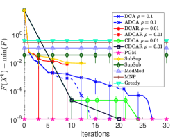
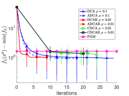
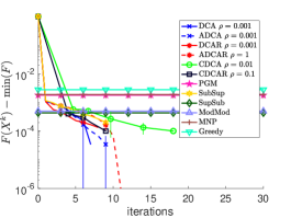
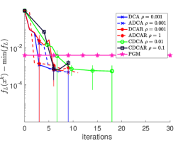
Figure 1: Discrete and continuous objective values (log-scale) vs iterations on speech (top) and mushroom (bottom) datasets.

In this section, we evaluate the empirical performance of our proposed methods on two applications: speech corpus selection and feature selection. We compare our proposed methods DCA, DCAR, CDCA and CDCAR to the state-of-the-art methods for DS minimization, SubSup, SupSub and ModMod (Narasimhan & Bilmes, 2005; Iyer & Bilmes, 2012). We also include an accelerated variant of DCA (ADCA) and DCAR (ADCAR), with the acceleration proposed in (Nhat et al., 2018). We use the minimum norm point (MNP) algorithm (Fujishige & Isotani, 2011) for submodular minimization in SubSup and the optimal Greedy algorithm of (Buchbinder et al., 2012, Algorithm 2) for submodular maximization in SupSub. We also compare with the MNP, PGM, and Greedy algorithms applied directly to the DS problem (1).

We do not restrict $\rho$ to zero or the iterates to be integral in DCA and CDCA (recall that DCA in this case reduces to SubSup). Instead, we vary $\rho$ between $0$ and $10$, and round only once at convergence (though for evaluation purposes we do round at each iteration, but we do not update $x^{k+1}$ with the rounded iterate). We also do not consider $O(d)$ permutations for choosing $y^{k}$ in DCA, DCAR, SubSup and ModMod, as required in Corollary 3.2 and (Iyer & Bilmes, 2012) to guarantee convergence to an approximate local minimum of $F$, as this is too computationally expensive (unless done fully in parallel). Instead, we consider as in (Iyer & Bilmes, 2012) three permutations to break ties in $x^{k}$: a random permutation, a permutation ordered according to the decreasing marginal gains of $G$, i.e., $G(i\mid X^{k}\setminus i)$, or according to the decreasing marginal gains of $F$, i.e., $F(i\mid X^{k}\setminus i)$, which we try in parallel at each iteration, then pick the one yielding the best objective $F$. We also apply this heuristic in CDCA and CDCAR to choose an initial feasible point $w^{0}\in\rho x^{k}+\partial h_{L}(x^{k})$ for FW (12); we pick the permutation yielding the smallest objective $\phi_{k}(w^{0})$.

We use $f(x^{k})-f(x^{k+1})\leq 10^{-6}$ as a stopping criterion in our methods, and $X^{k+1}=X^{k}$ in SubSup, SupSub and ModMod as in (Iyer & Bilmes, 2012), and stop after a maximum number of iterations. To ensure convergence to a local minimum of $F$, we explicitly check for this as an additional stopping criterion in all methods except MNP, PGM and Greedy, and restart from the best neighboring set if not satisfied, as discussed in Section 3. For more details on the experimental set-up, see Appendix B. The code is available at https://github.com/SamsungSAILMontreal/difference-submodular-min.git.

Speech corpus selection

The goal of this problem is to find a subset of a large speech data corpus to rapidly evaluate new and expensive speech recognition algorithms. One approach is to select a subset of utterances $X$ from the corpus $V$ that simultaneously minimizes the vocabulary size and maximizes the total value of data (Lin & Bilmes, 2011; Jegelka et al., 2011). Also, in some cases, some utterances’ importance decrease when they are selected together. This can be modeled by minimizing $F(X)=\lambda\sqrt{|\mathcal{N}(X)|}-\sum_{i=1}^{r}\sqrt{m(X\cap V_{i})}$, where $\mathcal{N}(X)$ is the set of distinct words that appear in utterances $X$, $m$ is a non-negative modular function, with the weight $m_{j}$ representing the importance of utterance $j$, and $V_{1}\cup\cdots\cup V_{r}=V$. We can write $F$ as the difference of two non-decreasing submodular functions $G(X)=\lambda\sqrt{|\mathcal{N}(X)|}$ and $H(X)=\sum_{i}\sqrt{m(X\cap V_{i})}$. Moreover, this problem is a special case of DS minimization, where $H$ is approximately modular. In particular, $H$ is $(1,\beta)$-weakly DR-modular (see Definition H.1) with

$$\beta\geq\min_{i\in[r]}\min_{j\in V_{i}}\tfrac{1}{2}\sqrt{\tfrac{m(j)}{m(V_{i})}}.$$

The parameter $\beta$ characterizes how close $H$ is to being supermodular. This DS problem thus fits under the setting considered in (El Halabi & Jegelka, 2020) (with $\alpha=1$), for which PGM was shown to achieve the optimal approximation guarantee $F(\hat{X})\leq G(X^{*})-\beta H(X^{*})+\epsilon$ for some $\epsilon>0$, where $X^{*}$ is a minimizer of $F$ (see Corollary 1 and Theorem 2 therein). We show in Section H.1 that any variant of DCA and CDCA obtains the same approximation guarantee as PGM (see Proposition H.6 and discussion below it).
We use the same dataset used by (Bach, 2013, Section 12.1), with $d=|V|=800$ utterances and $1105$ words. We choose $\lambda=1$, the non-negative weights $m_{i}$ randomly, and partition $V$ into $r=10$ groups of consecutive indices.

Feature selection

Given a set of features $U_{V}=\{U_{1},U_{2},\cdots,U_{d}\}$, the goal is to find a small subset of these features $U_{X}=\{U_{i}:i\in X\}$ that work well when used to classify a class $C$. We thus want to select the subset which retains the most information from the original set $U_{V}$ about $C$. This can be modeled by minimizing $F(X)=\lambda|X|-\mathrm{I}(U_{X};C)$. The mutual information $\mathrm{I}(U_{X};C)$ can be written as the difference of the entropy $\mathcal{H}(U_{X})$ and conditional entropy $\mathcal{H}(U_{X}\mid C)$, both of which are non-decreasing submodular. Hence $F$ can be written as the difference of two non-decreasing submodular functions $G(X)=\lambda|X|+\mathcal{H}(U_{X}\mid C)$ and $H(X)=\mathcal{H}(U_{X})$. We estimate the mutual information from the data. We use the Mushroom data set from (Dua & Graff, 2017), which has 8124 instances with 22 categorical attributes, which we convert to $d=118$ binary features. We randomly select $70\%$ of the data as training data for the feature selection, and set $\lambda=10^{-4}$.

Results:

We plot in Fig. 1, the discrete objective values $F(X^{k})-\min(F)$ and continuous objective values $f_{L}(x^{k})-\min(f_{L})$, per iteration $k$, where $\min(F)$ and $\min(f_{L})$ are the smallest values achieved by all compared methods. We only plot the continuous objective of the methods which minimize the continuous DC problem (2), instead of directly minimizing the DS problem (1), i.e., our methods and PGM. For DCAR and CDCAR, we plot the continuous objective values before rounding, i.e., $f_{L}(\tilde{x}^{k})$, since the continuous objective after rounding is equal to the discrete one, i.e., $f_{L}({x}^{k})=F(X^{k})$. Results are averaged over 3 random runs, with standard deviations shown as error bars. For clarity, we only include our methods with the $\rho$ value achieving the smallest discrete objective value. We show the results for all $\rho$ values in Section C.1. For a fair implementation-independent comparison, we use the number of FW (12) iterations as the x-axis for CDCA and CDCAR, since one iteration of FW has a similar cost to an iteration of DCA variants. We only show the minimum objective achieved by SupSub, ModMod, MNP, PGM and Greedy, since their iteration time is significantly smaller than the DCA and CDCA variants. We show the results with respect to time in Section C.2.

We observe that, as expected, PGM obtains the same discrete objective value as the best variants of our methods on the speech dataset, where PGM and our methods achieve the same approximation guarantee, but worse on the adult dataset, where PGM has no guarantees. Though in terms of continuous objective value, PGM is doing worse than our methods on both datasets. Hence, a better $f_{L}$ value does not necessarily yield a better $F$ value after rounding. In both experiments, our methods reach a better $F$ value than all other baselines, except SubSup which gets the same value as DCAR on the speech dataset, and a similar value to our non-accelerated methods on the mushroom dataset.

The complete variants of our methods, CDCA and CDCAR, perform better in terms of $F$ values, than their simple counterparts, DCA and DCAR, on the speech dataset. But, on the mushroom dataset, CDCAR perform similarly to DCAR, while CDCA is worse that DCA. Hence, using the complete variant is not always advantageous. In terms of $f_{L}$ values, CDCA and CDCAR perform worse than DCA and DCAR, respectively, on both datasets. Again this illustrates than a better $f_{L}$ value does not always yield a better $F$ value.

Rounding at each iteration helps for CDCA on both datasets; CDCAR converges faster than CDCA in $F$, but not for DCA; DCAR reaches worse $F$ value than DCA. Note that unlike $f_{L}({x}^{k})$, the objective values $f_{L}(\tilde{x}^{k})$ of DCAR and CDCAR are not necessarily approximately non-increasing (Theorem E.5-b does not apply to them), which we indeed observe on the mushroom dataset.

Finally, we observe that adding regularization leads to better $F$ values; the best $\rho$ is non-zero for all our methods (see Section C.1 for a more detailed discussion on the effect of regularization). Acceleration helps in most cases but not all; DCAR and ADCAR perform the same on the speech dataset.

6 Conclusion

We introduce variants of DCA and CDCA for minimizing the DC program equivalent to DS minimization. We establish novel links between the two problems, which allow us to match the theoretical guarantees of existing algorithms using DCA, and to achieve stronger ones using CDCA. Empirically, our proposed methods perform similarly or better than all existing methods.

Appendix A Subsup as a Special Case of DCA

We show that the SubSup procedure proposed in (Narasimhan & Bilmes, 2005) is a special case of DCA. SubSup starts from $X^{0}\subseteq V$, and makes the following updates at each iteration:

$$y^{k}_{\sigma(i)} \leftarrow H(\sigma(i)\mid S^{\sigma}_{i-1})~{}\forall i\in V,\text{for }\sigma\in S_{d}\text{ such that }S^{\sigma}_{|X^{k}|}=X^{k}$$ (14)

$$X^{k+1} \leftarrow\mathop{{\rm argmin}}_{X\subseteq V}G(X)-y^{k}(X)$$

Note that $y^{k}\in\partial h_{L}(\mathds{1}_{X^{k}})$ by Proposition 2.3-f and $\mathds{1}_{X^{k+1}}\in\mathop{{\rm argmin}}_{x\in[0,1]^{d}}g_{L}(x)-\langle x,\,y^{k}\rangle$ as discussed in Section 3, thus they are valid updates of DCA in Eq. 7 with $\rho=\epsilon_{x}=0$.

Appendix B Experimental Setup Additional Details

Table 1: Stopping criteria

DCA, DCAR, CDCA, CDCAR SubSup SupSub, ModMod MNP, PGM PGM in DCA and MNP in SubSup FW in CDCA ADCA, ADCAR CDCA variants variants $f(x^{k})-f(x^{k+1})\leq 10^{-6}$ $f(x^{k})-f(x^{k+1})\leq 10^{-6}$ $X^{k+1}=X^{k}$ $X^{k+1}=X^{k}$ $\text{gap}\leq 10^{-6}$ $\text{gap}\leq 10^{-6}$ $\text{gap}\leq 10^{-6}$ $k\leq 30$ $k+\text{\# FW iterations}\leq 30$ $k\leq 30$ $k\leq 3\times 10^{4}$ $k\leq 3\times 10^{4}$ $k\leq 10^{3}$ $k\leq 10^{3}$ $k\leq 10$ $X^{k+1}$ local minimum of $F$ $X^{k+1}$ local minimum of $F$ $X^{k+1}$ local minimum of $F$ $X^{k+1}$ local minimum of $F$

In this section, we provide additional details on our experimental setup. As in (Iyer & Bilmes, 2012), we consider in ModMod and SupSub two modular upper bounds on $G$, which we try in parallel and pick the one which yields the best objective $F$. We set the parameter $q$ in ADCA and ADCAR to $5$ as done in (Nhat et al., 2018). We summarize the stopping criteria used in all methods and their subsolvers in Table 1. We pick the maximum number of iterations according to the complexity per iteration. We use the random seeds 42, 43, and 44. We use the implementation of MNP from the Matlab code provided in (Bach, 2013, Section 12.1) and implement the rest of the methods in Matlab.

Appendix C Additional Empirical Results

In this section, we present some additional empirical results of the experiments presented in Section 5.

C.1 Effect of regularization

color=red!30, inline] Recall here the theoretical effects of $\rho$. I think we can show that critical points of $g-h$ with $rho>0$ are critical points of $g-h$ without $\rho$ with $\epsilon$ depending on $\rho$ in the same was as for local minimality w.r.t $F$, which would explain maybe why overall larger $\rho$ leads to slower convergence.

We report the discrete and continuous objective values per iteration of our proposed methods, for all $\rho$ values, on the speech dataset in Fig. 2 and the mushroom dataset in Fig. 3. We observe that the variants without rounding at each iteration converge slower in $f_{L}$ for larger $\rho$ values, though not always, e.g., DCA with $\rho=0.001$ converges faster than with $\rho=0$ on the speech dataset, and CDCA with $\rho=0.01$ converges faster than with $\rho=0.1$ on the mushroom dataset. The effect of $\rho$ on the rounded variants is less clear; in most cases the methods with small $\rho$ values are performing worse, but for CDCAR on the speech dataset the opposite is true. We again observe that better performance w.r.t $f_{L}$ does not necessarily translate to better performance w.r.t $F$. The effect of $\rho$ on performance w.r.t $F$ varies with the different methods and datasets. But in all cases, the best $F$ values is obtained with $\rho>0$.

Recall that we use PGM to compute an $\epsilon_{x}$-subgradient of $g^{*}$ to update $x^{k}$ in DCA variants (7b) and CDCA variants (5b), as well as in each iteration of FW (12) to update $y^{k}$ in CDCA variants (5a). As discussed in Section 3, PGM requires $O(d\kappa^{2}/\epsilon_{x}^{2})$ iterations when $\rho=0$ and $O(2(\kappa+\rho\sqrt{d})^{2}/\rho\epsilon_{x})$ when $\rho>0$, where $\kappa$ is the Lipschitz constant of $g_{L}(x)-\langle x,\,y^{k}\rangle$. Figure 4 shows the gap reached by PGM at each iteration of DCA variants, and the worst gap reached by PGM over all the approximate subgradient computations done at each iteration of CDCA variants. As expected, a larger $\rho$ leads to a more accurate solution (smaller gap), for a fixed number of PGM iterations (we used $1000$). Though, the accuracy at $\rho=0$ is better than the very small non-zero values $\rho=0.01,0.001$, for which the complexity $O(2(\kappa+\rho\sqrt{d})^{2}/\rho\epsilon_{x})$ becomes larger than $O(d\kappa^{2}/\epsilon_{x}^{2})$.

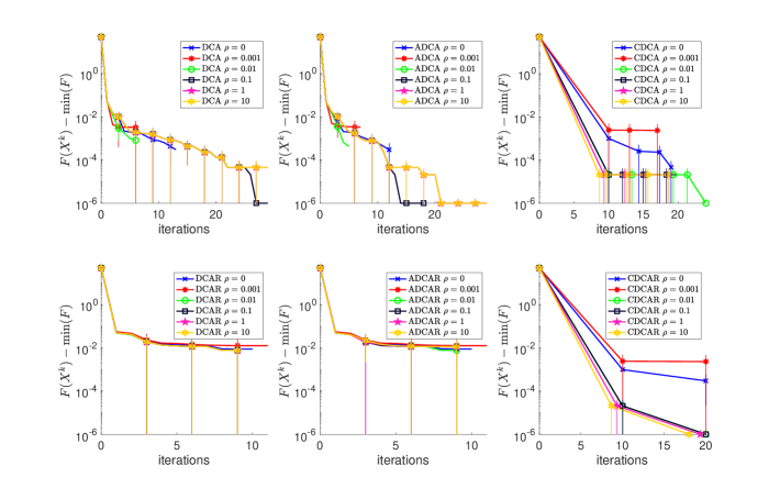
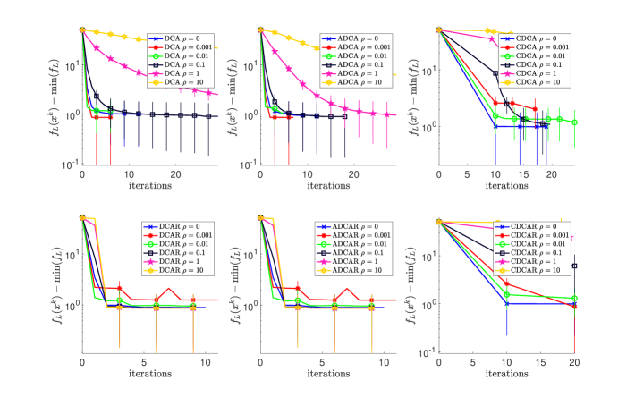
Figure 2: Discrete and continuous objective values (log-scale) of our proposed methods for all $\rho$ values vs iterations on speech dataset.

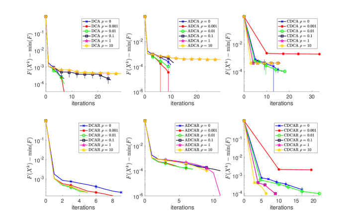
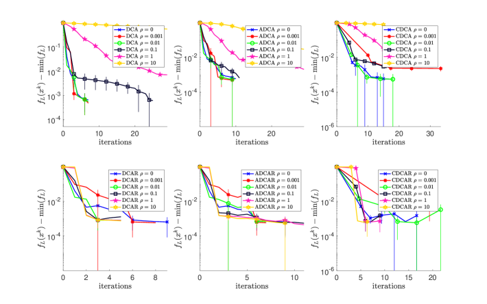
Figure 3: Discrete and continuous objective values (log-scale) of our proposed methods for all $\rho$ values vs iterations on mushroom dataset.

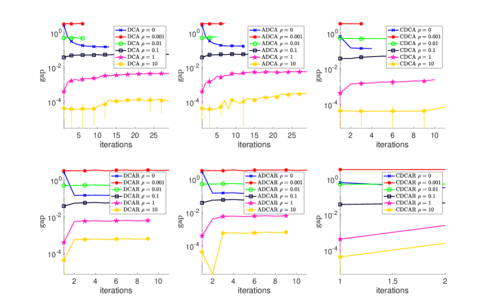
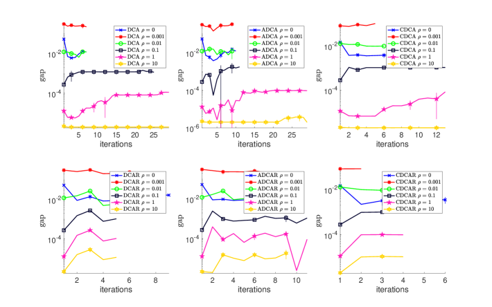
Figure 4: PGM gap values (log-scale) of our proposed methods for all $\rho$ values vs iterations on speech (top two rows) and mushroom (bottom two rows) datasets.

C.2 Running times

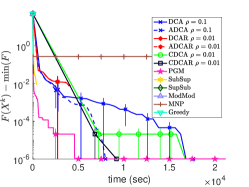
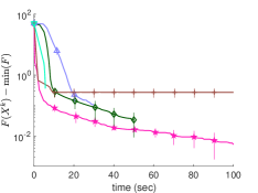
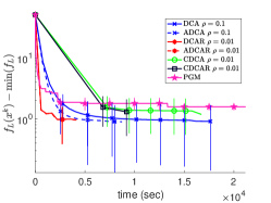
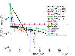
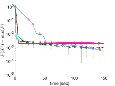
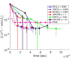
Figure 5: Discrete and continuous objective values (log-scale) vs time on speech (top) and mushroom (bottom) datasets. We include separate plots for non-DCA variants for visibility.

We report in Fig. 5 the discrete and continuous objective values with respect to time. We again only include our methods with the $\rho$ value achieving the smallest discrete objective. As expected, DCA variants (including SubSup) have a significantly higher computational cost compared to other baselines.

Recall that SubSup is a special case of DCA with $\rho=0$ and $x^{k}$ chosen to be integral (see Appendix A and the computational complexity discussion in Section 3), so theoretically the cost of SubSup is the same as DCA with $\rho=0$. In our experiments, we are using the MNP algorithm for the submodular minimization in SubSup $\min_{X\subseteq V}G(X)-y^{k}(X)=\min_{x\in[0,1]^{d}}g_{L}(x)-\langle x,\,y^{k}\rangle$, and PGM to solve Problem (7b) $\min_{x\in[0,1]^{d}}g_{L}(x)-\langle x,\,y^{k}\rangle+\tfrac{\rho}{2}\|x\|^{2}$ in DCA (MNP cannot be used for this problem when $\rho>0$). MNP requires $O({d~{}\mathrm{diam}\,(B(G-y^{k}))^{2}}/{\epsilon_{x}^{2}})$ iterations to obtain an $\epsilon_{x}$-solution to $\min_{X\subseteq V}G(X)-y^{k}(X)$ (Chakrabarty et al., 2014, Theorems 4 and 5). We can bound $\mathrm{diam}\,(B(G-y^{k}))\leq 2\kappa$, where recall that $\kappa$ is the Lipschitz constant of $g_{L}(x)-\langle x,\,y^{k}\rangle$ given in Proposition 2.3-g. Hence MNP requires the same number of iterations $O(d\kappa^{2}/\epsilon_{x}^{2})$ as PGD with $\rho=0$, and the time per iteration of MNP is $O(d^{2}+d\log d+d~{}\text{EO}_{G})$ (Chakrabarty et al., 2014, Proof of Theorem 1), which is larger than PGD $O(d\log d+d~{}\text{EO}_{G})$ (see the computational complexity discussion in Section 3). Nevertheless, in our experiments, we observe that SubSup actually has a lower running time per iteration than DCA on the speech dataset; this is true even for DCA with $\rho=0$ (see Fig. 6), but similar on the mushroom dataset.

C.3 SubSup vs DCA and DCAR with $\rho=0$

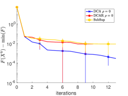
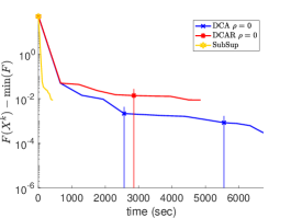
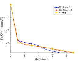
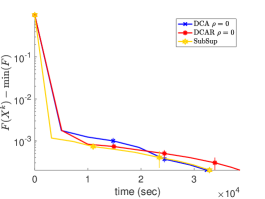
Figure 6: Discrete objective values (log-scale) of three DCA variants with $\rho=0$, vs iterations (left) and time (right), on speech (top) and mushroom (bottom) datasets.

In this section, we compare the performance of SubSup with DCA and DCAR with $\rho=0$. We plot the discrete objective values of these three algorithms with respect to both iterations and time in Fig. 6. We observe that SubSup performs similarly to DCAR with $\rho=0$ in terms of $F$ values, while DCA with $\rho=0$ obtains a bit better $F$ values on the speech dataset. Note that the only difference between SubSup and DCA with $\rho=0$ is that SubSup is choosing an integral solution in Problem (7b), using the MNP algorithm, while DCA chooses a possibly non-integral solution using the PGM algorithm. Hence, it seems that there is some advantage to not restricting the $x^{k}$ iterates of DCA to be integral in some cases. In terms of running time, SubSup has a lower iteration time than the other two algorithms on the speech dataset, and a similar one on the mushroom dataset (see discussion in Section C.2).

Appendix D Proofs of Section 2

D.1 Proof of Proposition 2.7

See 2.7

Proof.

1. The first part is an extension of (Le Thi & Pham Dinh, 1997, Theorem 4). Given $y\in\partial_{\epsilon_{1}}g(\hat{x})\cap\partial_{\epsilon_{2}}h(x)$, we have $g(\hat{x})+\langle y,\,x-\hat{x}\rangle-\epsilon_{1}\leq g(x)$ and $h(x)+\langle y,\,\hat{x}-x\rangle-\epsilon_{2}\leq h(\hat{x})$. Hence, $g(\hat{x})-h(\hat{x})\leq g(x)-h(x)+\epsilon_{1}+\epsilon_{2}$. If $\hat{x}$ admits a neighbourhood where this is true, then $\hat{x}$ is an $\epsilon$-local minimum of $g-h$. The converse direction extends a well known property; see e.g., (Hiriart-Urruty, 1989, Proposition 3.1). Given an $\epsilon$-local minimum $\hat{x}$ of $g-h$, there exists a neighborhood $U$ of $\hat{x}$ such that $g(\hat{x})-h(\hat{x})\leq g(x)-h(x)+\epsilon$ for all $x\in U$. Then for any $\hat{y}\in\partial h(\hat{x})$, $g(x)-g(\hat{x})\geq h(x)-h(\hat{x})-\epsilon\geq\langle\hat{y},\,x-\hat{x}\rangle-\epsilon$ for all $x\in U$. This is enough to have $\hat{y}\in\partial_{\epsilon}g(\hat{x})$, since for any $x\in\mathbb{R}^{d}$, we can apply the inequality to $x^{\prime}=\hat{x}+\tau(x-\hat{x})$ with $\tau>0$ small enough to have $x^{\prime}\in U$, then by convexity we get $\tau g(x)+(1-\tau)g(\hat{x})-g(\hat{x})\geq g(\hat{x}+\tau(x-\hat{x}))-g(\hat{x})\geq\langle\hat{y},\,\hat{x}+\tau(x-\hat{x})-\hat{x}\rangle-\epsilon$, which implies $g(x)-g(\hat{x})\geq\langle\hat{y},\,x-\hat{x}\rangle-\epsilon$. Hence, $\partial h(\hat{x})\subseteq\partial_{\epsilon}g(\hat{x})$.

2. This is an extension of (Le Thi & Pham Dinh, 1997, Corollary 2). If $h$ is locally polyhedral convex then for every $x\in\mathrm{dom}\,h$ there exists a neighborhood $U$ of $x$ such that $\partial h(x^{\prime})\subseteq\partial h(x)$ for all $x^{\prime}\in U$ (Le Thi & Pham Dinh, 1997, Theorem 5). Given $\hat{x}$ satisfying $\partial h(\hat{x})\subseteq\partial_{\epsilon}g(\hat{x})$, we have that $\partial h(x)\subseteq\partial_{\epsilon}g(\hat{x})$ for all $x\in U$ for some neighborhood $U$ of $x$, which implies that $\hat{x}$ is an $\epsilon$-local minimum of $g-h$ by Item a. The converse direction also follows from Item a.

∎

Remark D.1.

Let $\mathrm{ri}\,(S)$ denote the relative interior of a convex set $S$. Note that any $x\in\mathrm{ri}\,(\mathrm{dom}\,g)\cap\mathrm{ri}\,(\mathrm{dom}\,h)$ (which is equal to $\mathrm{ri}\,(\mathrm{dom}\,g)$ since we assumed $\min_{x}g(x)-h(x)$ is finite) is an $\epsilon$-local minimum of $g-h$ for any $\epsilon>0$. Hence, $\epsilon$-local minimality is meaningless on $\mathrm{ri}\,\mathrm{dom}\,g\cap\mathrm{ri}\,\mathrm{dom}\,h$ for any $\epsilon>0$. However, in this work, we are interested in integral $\epsilon$-local minima of Problem (2), which are on the boundary of $\mathrm{dom}\,(g_{L}+\delta_{[0,1]^{d}})=[0,1]^{d}$, and hence not meaningless.

Proof.

Since $g,h$ are convex, they are continuous on $\mathrm{ri}\,(\mathrm{dom}\,g)\cap\mathrm{ri}\,(\mathrm{dom}\,h)$ (Rockafellar, 1970, Theorem 10.1). This implies that $f$ is also continuous on $\mathrm{ri}\,(\mathrm{dom}\,g)\cap\mathrm{ri}\,(\mathrm{dom}\,h)$, hence for any $x\in\mathrm{ri}\,(\mathrm{dom}\,g)\cap\mathrm{ri}\,(\mathrm{dom}\,h)$, any $\epsilon>0$, there exists $\delta>0$, such that for all $x^{\prime}\in ri(\mathrm{dom}\,g)\cap\mathrm{ri}\,(\mathrm{dom}\,h)$ satisfying $\|x^{\prime}-x\|<\delta$, we have $|f(x^{\prime})-f(x)|<\epsilon$, hence $f(x)<f(x^{\prime})+\epsilon$. ∎

Appendix E Proofs of Section 3

E.1 Proof of Theorem 3.1

Before proving Theorem 3.1, we need the following lemma.

Lemma E.1 (Lemma 5 in (Pham Dinh et al., 2022)).

Let $\Phi$ be a $\rho$-strongly convex function with $\rho\geq 0$, then for any $\epsilon\geq 0$, $t\in(0,1],x\in\mathrm{dom}\,\Phi$ and $y\in\partial_{\epsilon}\Phi(x)$, we have

$$\Phi(z)\geq\Phi(x)+\langle y,\,z-x\rangle+\frac{\rho(1-t)}{2}\|z-x\|^{2}-\frac{\epsilon}{t},\quad\forall z\in\mathbb{R}^{d}.$$

We now present a more detailed version of Theorem 3.1 and its proof.

Theorem E.2.

Given any $f=g-h$, where $g,h\in\Gamma_{0}$, let $\{x^{k}\}$ and $\{y^{k}\}$ be generated by approximate DCA (Algorithm 1), and define $T_{\Phi}(x^{k+1})=\Phi(x^{k})-\Phi(x^{k+1})-\langle y^{k},x^{k}-x^{k+1}\rangle$ for any $\Phi\in\Gamma_{0}$, Then for all $t_{x},t_{y}\in(0,1],k\in\mathbb{N}$, let $\bar{\rho}=\rho(g)(1-t_{x})+\rho(h)(1-t_{y})$ and $\bar{\epsilon}=\tfrac{\epsilon_{x}}{t_{x}}+\tfrac{\epsilon_{y}}{t_{y}}$, we have:

1. $T_{g}(x^{k+1})\geq\tfrac{\rho(g)(1-t_{x})}{2}\|x^{k}-x^{k+1}\|^{2}-\tfrac{\epsilon_{x}}{t_{x}}\text{ and }T_{h}(x^{k+1})\leq-\tfrac{\rho(h)(1-t_{y})}{2}\|x^{k}-x^{k+1}\|^{2}+\tfrac{\epsilon_{y}}{t_{y}}.$

   Moreover, for any $\epsilon\geq 0$, if $T_{g}(x^{k+1})\leq\epsilon$, then $x^{k}$ is an $(\epsilon+\epsilon_{x},\epsilon_{y})$-critical point of $g-h$, with $y^{k}\in\partial_{\epsilon+\epsilon_{x}}g(x^{k})\cap\partial_{\epsilon_{y}}h(x^{k})$, and $\tfrac{\rho(g)(1-t_{x})}{2}\|x^{k}-x^{k+1}\|^{2}\leq\tfrac{\epsilon_{x}}{t_{x}}+\epsilon$. Conversely, if $x^{k}\in\partial_{\epsilon+\epsilon_{x}}g^{*}(y^{k})$, then $T_{g}(x^{k+1})\leq\epsilon_{x}+\epsilon$.

   Similarly, if $T_{h}(x^{k+1})\geq-\epsilon$, then $x^{k+1}$ is an $(\epsilon_{x},\epsilon+\epsilon_{y})$-critical point of $g-h$, with $y^{k}\in\partial_{\epsilon_{x}}g(x^{k+1})\cap\partial_{\epsilon+\epsilon_{y}}h(x^{k+1})$, and $\tfrac{\rho(h)(1-t_{y})}{2}\|x^{k}-x^{k+1}\|^{2}\leq\tfrac{\epsilon_{y}}{t_{y}}+\epsilon$. Conversely, if $y^{k}\in\partial_{\epsilon+\epsilon_{y}}h(x^{k+1})$, then $T_{h}(x^{k+1})\geq-\epsilon_{y}-\epsilon$.

2. $\begin{aligned} f(x^{k})-f(x^{k+1})=T_{g}(x^{k+1})-T_{h}(x^{k+1})\geq\frac{\bar{\rho}}{2}\|x^{k}-x^{k+1}\|^{2}-\bar{\epsilon}.\end{aligned}$

3. For any $\epsilon\geq 0$, $f(x^{k})-f(x^{k+1})\leq\epsilon$ if and only if $T_{g}(x^{k+1})-T_{h}(x^{k+1})\leq\epsilon$. In this case, $x^{k}$ is an $(\epsilon_{1}+\epsilon_{x},\epsilon_{y})$-critical point of $g-h$, with $y^{k}\in\partial_{\epsilon_{1}+\epsilon_{x}}g(x^{k})\cap\partial_{\epsilon_{y}}h(x^{k})$, $x^{k+1}$ is an $(\epsilon_{x},\epsilon_{2}+\epsilon_{y})$-critical point of $g-h$, with $y^{k}\in\partial_{\epsilon_{x}}g(x^{k+1})\cap\partial_{\epsilon_{2}+\epsilon_{y}}h(x^{k+1})$, for some $\epsilon_{1}+\epsilon_{2}=\epsilon,\epsilon_{1}\geq-\epsilon_{x},\epsilon_{2}\geq-\epsilon_{y}$, and $\frac{\bar{\rho}}{2}\|x^{k}-x^{k+1}\|^{2}\leq\bar{\epsilon}+\epsilon$. Conversely, if $x^{k}\in\partial_{\epsilon_{x}+\epsilon_{1}}g^{*}(y^{k})$ and $y^{k}\in\partial_{\epsilon_{y}+\epsilon_{2}}h(x^{k+1})$, then $T_{g}(x^{k+1})-T_{h}(x^{k+1})\leq\epsilon_{x}+\epsilon_{y}+\epsilon$ and $f(x^{k})-f(x^{k+1})\leq\epsilon_{x}+\epsilon_{y}+\epsilon$.

4. $\begin{aligned} \min_{k\in\{0,1,\dots,K-1\}}T_{g}(x^{k+1})-T_{h}(x^{k+1})=\min_{k\in\{0,1,\dots,K-1\}}f(x^{k})-f(x^{k+1})\leq\frac{f(x^{0})-f^{\star}}{K}.\end{aligned}$

5. If $\rho(g)+\rho(h)>0$, then

   $$\min_{k\in\{0,1,\dots,K-1\}}\|x^{k}-x^{k+1}\|\leq\sqrt{\frac{2}{\bar{\rho}}\big{(}\frac{f(x^{0})-f^{\star}}{K}+\bar{\epsilon}\big{)}.}$$

Proof.

1. Since $x^{k+1}\in\partial_{\epsilon_{x}}g^{*}(y^{k})$, then $y^{k}\in\partial_{\epsilon_{x}}g(x^{k+1})$ by Proposition 2.4. By Lemma E.1 we have for all $x\in\mathbb{R}^{d}$

   $$g(x)\geq g(x^{k+1})+\langle y^{k},\,x-x^{k+1}\rangle+\tfrac{\rho(g)(1-t_{x})}{2}\|x-x^{k+1}\|^{2}-\tfrac{\epsilon_{x}}{t_{x}},$$ (15)

   hence $T_{g}(x^{k+1})\geq\tfrac{\rho(g)(1-t_{x})}{2}\|x^{k}-x^{k+1}\|^{2}-\tfrac{\epsilon_{x}}{t_{x}}$. If $T_{g}(x^{k+1})\leq\epsilon$, taking $t_{x}=1$ in (15), we have for all $x\in\mathbb{R}^{d}$

   $$g(x)\geq g(x^{k})-\langle y^{k},x^{k}-x^{k+1}\rangle-\epsilon+\langle y^{k},\,x-x^{k+1}\rangle-\epsilon_{x}\geq g(x^{k})+\langle y^{k},x-x^{k}\rangle-\epsilon-\epsilon_{x},$$

   so $y^{k}\in\partial_{\epsilon+\epsilon_{x}}g(x^{k})\cap\partial_{\epsilon_{y}}h(x^{k})$ and $x^{k}$ is an $(\epsilon+\epsilon_{x},\epsilon_{y})$-critical point. Similarly, since $y_{k}\in\partial_{\epsilon_{y}}h(x^{k})$, we have for all $x\in\mathbb{R}^{d}$

   $$h(x)\geq h(x^{k})+\langle y^{k},\,x-x^{k}\rangle+\tfrac{\rho(h)(1-t_{y})}{2}\|x-x^{k}\|^{2}-\tfrac{\epsilon_{y}}{t_{y}},$$ (16)

   hence $T_{h}(x^{k+1})\leq-\tfrac{\rho(g)(1-t_{y})}{2}\|x^{k}-x^{k+1}\|^{2}+\tfrac{\epsilon_{y}}{t_{y}}$. If $T_{h}(x^{k+1})\geq-\epsilon$, taking $t_{y}=1$ in (16), we have for all $x\in\mathbb{R}^{d}$

   $$h(x)\geq h(x^{k+1})+\langle y^{k},x^{k}-x^{k+1}\rangle-\epsilon+\langle y^{k},\,x-x^{k}\rangle-\epsilon_{y}\geq h(x^{k+1})+\langle y^{k},x-x^{k+1}\rangle-\epsilon-\epsilon_{y},$$

   so $y^{k}\in\partial_{\epsilon_{x}}g(x^{k+1})\cap\partial_{\epsilon+\epsilon_{y}}h(x^{k+1})$ and $x^{k+1}$ is an $(\epsilon_{x},\epsilon+\epsilon_{y})$-critical point. The converse directions follow directly from the definitions of approximate subdifferentials and $T_{\Phi}$.

2. We have

   $$f(x^{k})-f(x^{k+1}) =g(x^{k})-g(x^{k+1})+\langle y^{k},\,x^{k}-x^{k+1}\rangle-(h(x^{k})-h(x^{k+1})+\langle y^{k},\,x^{k}-x^{k+1}\rangle)$$

   $$=T_{g}(x^{k+1})-T_{h}(x^{k+1})$$

   $$\geq\tfrac{\bar{\rho}}{2}\|x^{k}-x^{k+1}\|^{2}-\bar{\epsilon},$$

   where the inequality follows from Item a.

3. This follows from Items a and b, by choosing $\epsilon_{1}\geq T_{g}(x^{k+1})$ and $\epsilon_{2}\geq-T_{h}(x^{k+1})$.

4. This follows from Item b by telescoping sum:

   $$\min_{k\in\{0,1,\dots,K-1\}}T_{g}(x^{k+1})-T_{h}(x^{k+1}) =\min_{k\in\{0,1,\dots,K-1\}}f(x^{k})-f(x^{k+1})$$

   $$\leq\tfrac{1}{K}\sum_{k=0}^{K-1}T_{g}(x^{k+1})-T_{h}(x^{k+1})$$

   $$=\tfrac{1}{K}\sum_{k=0}^{K-1}f(x^{k})-f(x^{k+1})$$

   $$=\frac{f(x^{0})-f(x^{K})}{K}\leq\frac{f(x^{0})-f^{\star}}{K}.$$

5. This follows from Items b and d.

   $$\min_{k\in\{0,1,\dots,K-1\}}\|x^{k}-x^{k+1}\|^{2}\leq\min_{k\in\{0,1,\dots,K-1\}}\frac{2}{\bar{\rho}}(f(x^{k})-f(x^{k+1})+\bar{\epsilon})\leq\frac{2}{\bar{\rho}}\big{(}\frac{f(x^{0})-f^{\star}}{K}+\bar{\epsilon}\big{)}.$$

∎

Note that $f(x^{k})-f(x^{k+1})$ acts as a measure of non-criticality, since $f(x^{k})=f(x^{k+1})$ implies that $x^{k}$ and $x^{k+1}$ are critical points, when $\epsilon_{x}=\epsilon_{y}=0$. Theorem E.2 also motivates $\min\{T_{g}(x^{k+1}),T_{h}(x^{k})\}$ as a weaker measure of non-criticality, since $\min\{T_{g}(x^{k+1}),T_{h}(x^{k})\}=0$ implies that $x^{k}$ is a critical point, when $\epsilon_{x}=\epsilon_{y}=0$. Items d and a imply the following bound

$$\min_{k\in\{0,1,\dots,K-1\}}\min\{T_{g}(x^{k+1}),T_{h}(x^{k})\}\leq\min\{\tfrac{f(x^{0})-f^{\star}}{K}+\epsilon_{y},\tfrac{f(x^{0})-f^{\star}}{K-1}+\epsilon_{x}\},$$

which recovers the convergence rate provided in (Abbaszadehpeivasti et al., 2021, Corollary 4.1) on $T_{g}(x^{k+1})$, with $\epsilon_{x}=\epsilon_{y}=0$. The criterion $T_{g}(x^{k+1})\leq\epsilon$ has also been used as a stopping criterion of FW for nonconvex problems; see Section F.1 and (Ghadimi, 2019, Eq. (2.6)).

E.2 Proof of Corollary 3.2

Before proving Corollary 3.2, we need the following lemma.

Lemma E.3.

Let $\Phi$ be a convex function with bounded domain of diameter $D$, i.e., $\|x-z\|\leq D$ for all $x,z\in\mathrm{dom}\,\Phi$, and $\tilde{\Phi}=\Phi+\frac{\rho}{2}\|\cdot\|^{2}$ for some $\rho\geq 0$. Then for any $x\in\mathrm{dom}\,\Phi$, if $y-\rho x\in\partial_{\epsilon}\Phi(x)$, then $y\in\partial_{\epsilon}\tilde{\Phi}(x)$. Conversely, if $y\in\partial_{\epsilon}\tilde{\Phi}(x)$, then $y-\rho x\in\partial_{\epsilon^{\prime}}\Phi(x)$, where $\epsilon^{\prime}=\sqrt{2\rho\epsilon}D$ if $\epsilon\leq\tfrac{\rho D^{2}}{2}$, and $\tfrac{\rho D^{2}}{2}+\epsilon$ otherwise.

Proof.

If $y-\rho x\in\partial_{\epsilon}\Phi(x)$, we have

$$\Phi(z) \geq\Phi(x)+\langle y-\rho x,\,z-x\rangle-\epsilon$$

$$\Leftrightarrow\Phi(z) \geq\Phi(x)+\langle y,\,z-x\rangle+\rho\|x\|^{2}-\langle\rho x,\,z\rangle+\tfrac{\rho}{2}\|z\|^{2}-\tfrac{\rho}{2}\|z\|^{2}-\epsilon$$

$$\Leftrightarrow\tilde{\Phi}(z) \geq\tilde{\Phi}(x)+\langle y,\,z-x\rangle+\tfrac{\rho}{2}\|x-z\|^{2}-\epsilon$$

$$\Rightarrow\tilde{\Phi}(z) \geq\tilde{\Phi}(x)+\langle y,\,z-x\rangle-\epsilon$$

Hence, $y\in\partial_{\epsilon}\tilde{\Phi}(x)$. Conversely, if $y\in\partial_{\epsilon}\tilde{\Phi}(x)$, then by Lemma E.1, we have for all $t\in(0,1],z\in\mathrm{dom}\,\Phi$

$$\tilde{\Phi}(z) \geq\tilde{\Phi}(x)+\langle y,\,z-x\rangle+\frac{\rho(1-t)}{2}\|z-x\|^{2}-\frac{\epsilon}{t}$$

$$\geq\tilde{\Phi}(x)+\langle y,\,z-x\rangle+\frac{\rho}{2}\|z-x\|^{2}-\frac{\rho t}{2}D^{2}-\frac{\epsilon}{t}$$

$$\Leftrightarrow{\Phi}(z) \geq{\Phi}(x)+\langle y-\rho x,\,z-x\rangle-\frac{\rho t}{2}D^{2}-\frac{\epsilon}{t}$$

Hence, $y-\rho x\in\partial_{\epsilon^{\prime}}\Phi(x)$ with $\epsilon^{\prime}=\min_{t\in(0,1)}\frac{\rho t}{2}D^{2}+\frac{\epsilon}{t}=\min\{\sqrt{2\rho\epsilon}D,\tfrac{\rho D^{2}}{2}+\epsilon\}$. ∎

See 3.2

Proof.

1. If $f(x^{k})-f(x^{k+1})\leq\epsilon$, we have by Theorem 3.1-b (with $\epsilon_{y}=0$) that $y^{k}\in\partial_{\epsilon_{x}+\epsilon}g(x^{k})$, which by Lemma E.3 implies that $y^{k}-\rho x^{k}\in\partial_{\epsilon^{\prime}}(g_{L}+\delta_{[0,1]^{d}})(x^{k})$, by taking $D=\max_{x,z\in\mathrm{dom}\,(g_{L}+\delta_{[0,1]^{d}})}\|x-z\|=\sqrt{d}$. We observe that for any $\ell\in V$, we have $y^{k}-\rho x^{k}\in\partial h_{L}(\mathds{1}_{S^{\sigma}_{\ell}})$ by Proposition 2.3-f. Hence, $\partial_{\epsilon^{\prime}}(g_{L}+\delta_{[0,1]^{d}})(x^{k})\cap\partial h_{L}(x)\not=0$, and by Proposition 2.7-a $f(x^{k})\leq f(\mathds{1}_{S^{\sigma}_{\ell}})+\epsilon^{\prime}$. The statement then follows by Proposition 2.3-a.

2. Note that $y^{k}_{\sigma_{i}},x^{k+1}_{\sigma_{i}}$ for any $i\in V$ are valid iterates for approximate DCA, so Item a apply to them. If $f(x^{k})-f(x^{k+1})\leq\epsilon$, then $f(x^{k})-f(x^{k+1}_{\sigma_{i}})\leq\epsilon$ since $f(x^{k+1})\leq f(x^{k+1}_{\sigma_{i}})$ for all $i\in V$. Hence, by Item a we have $F(X^{k})\leq F(S^{\sigma_{i}}_{\ell})+\epsilon^{\prime}$ for all $i,\ell\in V$. We now observe that for any $j\in X^{k}$ there exists $\sigma_{i}$ for some $i\in V$, such that $\sigma_{i}(|X^{k}|)=j$, and $S^{\sigma_{i}}_{|X^{k}|-1}=X^{k}\setminus j$. Similarly for any $j\in V\setminus X^{k}$, there exists $\sigma_{i}$ for some $i\in V$, such that $\sigma_{i}(|X^{k}|+1)=j$, and $S^{\sigma_{i}}_{|X^{k}|+1}=X^{k}\cup j$. Then $X^{k}$ is an $\epsilon^{\prime}$-local minimum of $F$.

∎

E.3 Convergence properties of DCA variants

In this section, we present convergence properties of the DCA variants discussed in Section 3. We start by the DCA variant presented in Algorithm 2, where at convergence we explicitly check if rounding the current iterate yields an $\epsilon^{\prime}$-local minimum of $F$, and if not we restart from the best neighboring set.

Algorithm 2 Approximate DCA with local minimality stopping criterion

1:  $\epsilon,\epsilon^{\prime},\epsilon_{x}\geq 0,x^{0}\in\mathrm{dom}\,\partial h$, $k\leftarrow 0$.

2:  for $k=1,2,\cdots,K$ do

3:     $y^{k}\in\partial h(x^{k})$

4:     $x^{k+1}\in\partial_{\epsilon_{x}}g^{*}(y^{k})$

5:     if $f(x^{k})-f(x^{k+1})\leq\epsilon$ then

6:        $X^{k+1}=\mathrm{Round}_{F}(x^{k+1})$

7:        if $X^{k+1}$ is an $\epsilon^{\prime}$-local minimum of $F$ then

8:           Stop

9:        else

10:           $x^{k+1}=\mathds{1}_{\hat{X}^{k+1}}$ where $\hat{X}^{k+1}=\mathop{{\rm argmin}}_{|X\Delta X^{k+1}|=1}F(X)$

11:        end if

12:     end if

13:  end for

Proposition E.4.

Given $f=g-h$ as defined in (6) and $\epsilon^{\prime}\geq\epsilon+\epsilon_{x}$, Algorithm 2 converges to an $\epsilon^{\prime}$-local minimum of $F$ after at most $(f(x^{0})-f^{\star})/\epsilon$ iterations.

Proof.

Note that between each restart (line 10), Algorithm 2 is simply running approximate DCA, so Theorem 3.1 applies. For any iteration $k\in\mathbb{N}$, if the algorithm did not terminate, then either $f(x^{k})-f(x^{k+1})>\epsilon$ or $X^{k+1}$ is not an $\epsilon^{\prime}$-local minimum of $F$ and thus $F(X^{k+1})>F(\hat{X}^{k+1})+\epsilon^{\prime}$. In the second case, we have

$$f(\mathds{1}_{\hat{X}^{k+1}})=F(\hat{X}^{k+1}) <F(X^{k+1})-\epsilon^{\prime}$$ (by Proposition 2.3-a)

$$\leq f(x^{k+1})-\epsilon^{\prime}$$ (by Proposition 2.3-d)

$$\leq f(x^{k})+\epsilon_{x}-\epsilon^{\prime} t_{x}=1,\epsilon_{y}=0$$ (by Theorem 3.1-a with )

$$\leq f(x^{k})-\epsilon \epsilon^{\prime}\geq\epsilon+\epsilon_{x}$$ (since )

Hence, the new $x^{k+1}=\mathds{1}_{\hat{X}^{k+1}}$ will satisfy $f(x^{k})-f(x^{k+1})>\epsilon$. Thus $f^{\star}<f(x^{k})<f(x^{0})-k\epsilon$ and $k<(f(x^{0})-f^{\star})/\epsilon$. ∎

Next we present convergence properties of approximate DCAR (10).

Theorem E.5.

Given $f=g-h$ as defined in (6), let $\{x^{k}\},\{X^{k}\},\{\tilde{x}^{k}\}$ and $\{y^{k}\}$ be generated by approximate DCAR (10), and define $T_{\Phi}(x^{k+1})=\Phi(x^{k})-\Phi(x^{k+1})-\langle y^{k},x^{k}-x^{k+1}\rangle$ for any $\Phi\in\Gamma_{0}$, Then for all $t_{x}\in(0,1],k\in\mathbb{N}$, we have:

1. $T_{g}(\tilde{x}^{k+1})\geq\tfrac{\rho(1-t_{x})}{2}\|x^{k}-\tilde{x}^{k+1}\|^{2}-\tfrac{\epsilon_{x}}{t_{x}}$, and $T_{h}(\tilde{x}^{k+1})\leq-\tfrac{\rho}{2}\|x^{k}-\tilde{x}^{k+1}\|^{2}$.

   Moreover, for any $\epsilon\geq 0$, if $T_{g}(\tilde{x}^{k+1})\leq\epsilon$, then $x^{k}$ is an $(\epsilon+\epsilon_{x},0)$-critical point of $g-h$, with $y^{k}\in\partial_{\epsilon+\epsilon_{x}}g(x^{k})\cap\partial h(x^{k})$, and $\tfrac{\rho(1-t_{x})}{2}\|x^{k}-\tilde{x}^{k+1}\|^{2}\leq\tfrac{\epsilon_{x}}{t_{x}}+\epsilon$. Conversely, if $x^{k}\in\partial_{\epsilon+\epsilon_{x}}g^{*}(y^{k})$, then $T_{g}(\tilde{x}^{k+1})\leq\epsilon_{x}+\epsilon$.

   Similarly, if $T_{h}(\tilde{x}^{k+1})\geq-\epsilon$, then $\tilde{x}^{k+1}$ is an $(\epsilon_{x},\epsilon)$-critical point of $g-h$, with $y^{k}\in\partial_{\epsilon_{x}}g(\tilde{x}^{k+1})\cap\partial_{\epsilon}h(\tilde{x}^{k+1})$, and $\tfrac{\rho}{2}\|x^{k}-\tilde{x}^{k+1}\|^{2}\leq\epsilon$. Conversely, if $y^{k}\in\partial_{\epsilon}h(\tilde{x}^{k+1})$, then $T_{h}(\tilde{x}^{k+1})\geq-\epsilon$.

2. $F(X^{k})-F(X^{k+1})$ $\geq f(x^{k})-f(\tilde{x}^{k+1})=T_{g}(\tilde{x}^{k+1})-T_{h}(\tilde{x}^{k+1})\geq\tfrac{\rho(2-t_{x})}{2}\|x^{k}-\tilde{x}^{k+1}\|^{2}-\tfrac{\epsilon_{x}}{t_{x}}$.

3. For any $\epsilon\geq 0,F(X^{k})-F(X^{k+1})\leq\epsilon$ then $f(x^{k})-f(\tilde{x}^{k+1})=T_{g}(\tilde{x}^{k+1})-T_{h}(\tilde{x}^{k+1})\leq\epsilon$. In this case, $x^{k}$ is an $(\epsilon_{x}+\epsilon_{1},0)$-critical point of $g-h$, with $y^{k}\in\partial_{\epsilon_{x}+\epsilon_{1}}g(x^{k})\cap\partial h(x^{k}),\tilde{x}^{k+1}$ is an $(\epsilon_{x},\epsilon_{2})$-critical point of $g-h$ with $y^{k}\in\partial_{\epsilon_{x}}g(\tilde{x}^{k+1})\cap\partial_{\epsilon_{2}}h(\tilde{x}^{k+1})$ for some $\epsilon_{1}+\epsilon_{2}=\epsilon,\epsilon_{1}\geq-\epsilon_{x},\epsilon_{2}\geq 0,$ and $\tfrac{\rho(2-t_{x})}{2}\|x^{k}-\tilde{x}^{k+1}\|^{2}\leq\epsilon+\tfrac{\epsilon_{x}}{t_{x}}$. Conversely, if $x^{k}\in\partial_{\epsilon_{x}+\epsilon_{1}}g^{*}(y^{k}),$ and $y^{k}\in\partial_{\epsilon_{2}}h(\tilde{x}^{k+1})$, then $T_{g}(\tilde{x}^{k+1})-T_{h}(\tilde{x}^{k+1})\leq\epsilon_{x}+\epsilon$ and $f(x^{k})-f(\tilde{x}^{k+1})\leq\epsilon_{x}+\epsilon$.

4. $\min_{k\in\{0,1,\dots,K-1\}}T_{g}(\tilde{x}^{k+1})-T_{h}(\tilde{x}^{k+1})=\min_{k\in\{0,1,\dots,K-1\}}f(x^{k})-f(\tilde{x}^{k+1})\leq$ $\min_{k\in\{0,1,\dots,K-1\}}F(X^{k})-F(X^{k+1})\leq\frac{F(X^{0})-F^{\star}}{K}$.

5. If $\rho>0$, then

   $$\min_{k\in\{0,1,\dots,K-1\}}\|x^{k}-\tilde{x}^{k+1}\|\leq\sqrt{\tfrac{2}{\rho(2-t_{x})}\big{(}\frac{F(X^{0})-F^{\star}}{K}+\tfrac{\epsilon_{x}}{t_{x}}\big{)}}.$$

Proof.

Note that the iterates $\tilde{x}^{k+1},y^{k}$ are generated by an approximate DCA step from $x^{k}$, so Theorem E.2 apply to them.

1. The claim follows from Theorem E.2-a.

2. By Theorem E.2-b, we have

   $$f(x^{k})-f(\tilde{x}^{k+1})=T_{g}(\tilde{x}^{k+1})-T_{h}(\tilde{x}^{k+1})\geq\tfrac{\rho(2-t_{x})}{2}\|x^{k}-\tilde{x}^{k+1}\|^{2}-\tfrac{\epsilon_{x}}{t_{x}}.$$

   By Proposition 2.3-a, we also have $F(X^{k})-F(X^{k+1})=f(x^{k})-f(x^{k+1})$. The claim then follows since $f(x^{k+1})\leq f(\tilde{x}^{k+1})$ by Proposition 2.3-d.

3. This follows from Item b and Theorem E.2-c.

4. This follows from Item b by telescoping sum.

5. This follows from Items b and d.

∎

Appendix F Proofs of Section 4

F.1 Proof of Corollary 4.1

See 4.1

Proof.

We observe that approximate FW with $\gamma_{t}=1$ is a special case of approximate DCA (1), with DC components

$$g^{\prime}=\delta_{\partial h(x^{k})}\text{ and }h^{\prime}=-\phi_{k},$$

and $\epsilon_{x}=0,\epsilon_{y}=\epsilon$. Indeed, we can write the approximate FW iterates $w^{0}\in\partial h(x^{k})=\mathrm{dom}\,\partial g^{\prime}$, $-s^{t}\in\partial_{\epsilon}h^{\prime}(w^{t})$ and $w^{t+1}=v^{t}\in\mathop{{\rm argmin}}_{w}g^{\prime}(w)-\langle-s^{t},\,w\rangle=\partial(g^{\prime})^{*}(-s^{t})$, which are valid iterates of approximate DCA (1).

We show also that $g^{\prime},h^{\prime}\in\Gamma_{0}$: We can assume w.l.o.g that $\partial h(x^{k})\not=\emptyset$, otherwise the bound holds trivially. Hence, $g^{\prime}$ is proper. And since $h\in\Gamma_{0}$, $\partial h(x^{k})$ is a closed and convex set, hence $g^{\prime}$ is a closed and convex function. We also have that $h^{\prime}$ is proper, since otherwise Problem (5a) would not have a finite minimum, which also implies that the minimum of the DC dual (4) is not finite, contradicing our assumption that the minimum of the DC problem (3) is finite. Finally, since the fenchel conjugate $g^{*}$ is closed and convex, then $h^{\prime}$ is also closed and convex.

We can thus apply Theorem E.2. We get

$$\min_{k\in\{0,1,\dots,K-1\}}T_{g^{\prime}}(w^{k+1})-T_{h^{\prime}}(w^{k+1}) \leq\frac{\phi(w^{0})-\min_{w\in\partial h(x^{k})}\phi_{k}(w)}{K}$$ (by Theorem E.2-d)

$$\Rightarrow\min_{k\in\{0,1,\dots,K-1\}}T_{g^{\prime}}(w^{k+1}) \leq\frac{\phi(w^{0})-\min_{w\in\partial h(x^{k})}\phi_{k}(w)}{K}+\epsilon t_{y}=1$$ (by Theorem E.2-a with )

The claim now follows by noting that $T_{g^{\prime}}(w^{t+1})=\langle s^{t},\,w^{t}-w^{t+1}\rangle=\mathrm{gap}(w^{t})$. ∎

F.2 Proof of Proposition 4.2

See 4.2

Proof.

By Proposition 2.3-f, $w\in\partial h_{L}(x)$, so it is a feasible solution. Given any $w^{\prime}\in\partial h_{L}(x)$, $w^{\prime}$ is a maximizer of $\max_{w\in B(H)}\langle w,\,s\rangle$, hence it must satisfy $w^{\prime}(C_{i})=H(C_{i})$ for all $i\in\{1,\cdots,m\}$ (Bach, 2013, Proposition 4.2). We have

$$\langle s,\,w-w^{\prime}\rangle =\sum_{i=1}^{m}\sum_{k=1}^{|A_{i}|}s_{\sigma(|C_{i-1}|+k)}\left(H(\sigma(|C_{i-1}|+k)\mid S^{\sigma}_{|C_{i-1}|+k-1})-w^{\prime}_{\sigma(|C_{i-1}|+k)}\right)$$

$$=\sum_{i=1}^{m}\left(\begin{multlined}\sum_{k=1}^{|A_{i}|-1}(s_{\sigma(|C_{i-1}|+k)}-s_{\sigma(|C_{i-1}|+k+1)})(H(S^{\sigma}_{|C_{i-1}|+k})-w^{\prime}(S^{\sigma}_{|C_{i-1}|+k}))\\ -s_{\sigma(|C_{i-1}|+1)}(H(S^{\sigma}_{|C_{i-1}|})-w^{\prime}(S^{\sigma}_{|C_{i-1}|}))+s_{\sigma(|C_{i}|)}(H(S^{\sigma}_{|C_{i}|})-w^{\prime}(S^{\sigma}_{|C_{i}|}))\end{multlined}\sum_{k=1}^{|A_{i}|-1}(s_{\sigma(|C_{i-1}|+k)}-s_{\sigma(|C_{i-1}|+k+1)})(H(S^{\sigma}_{|C_{i-1}|+k})-w^{\prime}(S^{\sigma}_{|C_{i-1}|+k}))\\ -s_{\sigma(|C_{i-1}|+1)}(H(S^{\sigma}_{|C_{i-1}|})-w^{\prime}(S^{\sigma}_{|C_{i-1}|}))+s_{\sigma(|C_{i}|)}(H(S^{\sigma}_{|C_{i}|})-w^{\prime}(S^{\sigma}_{|C_{i}|}))\right)$$

$$\geq 0.$$

The last inequality holds since $w^{\prime}\in B(H)$ and $S^{\sigma}_{|C_{i}|}=C_{i}$ for all $i\in\{1,\cdots,m\}$. ∎

F.3 Proof of Theorem 4.3

To prove Theorem 4.3 we need the following lemma, which extends the result in (Pham Dinh & Souad, 1988, Theorem 2.3).

Lemma F.1.

For any $\epsilon\geq 0$, $\hat{x}$ is an $\epsilon$-strong critical point of $g-h$ if and only if there exists $\hat{y}\in\mathop{{\rm argmin}}\{\langle y,\,\hat{x}\rangle-g^{*}(y):y\in\partial h(\hat{x})\}$ such that $\hat{x}\in\partial_{\epsilon}g^{*}(\hat{y})$.

Proof.

If $\hat{x}$ is an $\epsilon$-strong critical point of $g-h$, i.e., $\partial h(\hat{x})\subseteq\partial_{\epsilon}g(\hat{x})$, then for every $y\in\partial h(\hat{x})$, we have $y\in\partial_{\epsilon}g(\hat{x})$. In particular, this holds for $\hat{y}\in\mathop{{\rm argmin}}\{\langle y,\,\hat{x}\rangle-g^{*}(y):y\in\partial h(\hat{x})\}$, hence $\hat{x}\in\partial_{\epsilon}g^{*}(\hat{y})$ by Proposition 2.4. Conversely, given $\hat{y}\in\mathop{{\rm argmin}}\{\langle y,\,\hat{x}\rangle-g^{*}(y):y\in\partial h(\hat{x})\}$ such that $\hat{x}\in\partial_{\epsilon}g^{*}(\hat{y})$, we have

$$\langle\hat{y},\,\hat{x}\rangle-g^{*}(\hat{y})\leq\langle y,\,\hat{x}\rangle-g^{*}(y),\forall y\in\partial h(\hat{x}).$$ (17)

Since $\hat{x}\in\partial_{\epsilon}g^{*}(\hat{y})$, we have by Proposition 2.4, $g^{*}(\hat{y})+g(\hat{x})-\langle\hat{y},\,\hat{x}\rangle\leq\epsilon$. Combining this with (17) yields

$$g(\hat{x})-\epsilon\leq\langle y,\,\hat{x}\rangle-g^{*}(y),\forall y\in h(\hat{x}).$$

By definition of $g^{*}$, we obtain

$$g(\hat{x})-\epsilon\leq\langle y,\,\hat{x}-x\rangle+g(x),\forall x\in\mathbb{R}^{d},\forall y\in h(\hat{x}).$$

Hence $y\in\partial_{\epsilon}g(\hat{x})$ for all $y\in h(\hat{x})$. ∎

See 4.3

Proof.

Since approximate CDCA is a special case of approximate DCA, with $\epsilon_{y}=0$, Theorem 3.1 applies. If $f(x^{k})-f(x^{k+1})\leq\epsilon$, we have by Theorem 3.1-b that $x^{k}\in\partial_{\epsilon_{x}+\epsilon}g^{*}(y^{k})$. Hence, by Lemma F.1 $x^{k}$ satisfies $\partial h(x^{k})\subseteq\partial_{\epsilon_{x}+\epsilon}g(x^{k})$. If $h$ is locally polyhedral, this implies that $x^{k}$ is an $(\epsilon+\epsilon_{x})$-local minimum of $f$ by Proposition 2.7-b. ∎

F.4 Proof of Corollary 4.4

See 4.4

Proof.

Assume that $\hat{x}$ is an $\epsilon$-strong critical point of $g-h$. We first observe that any vector $x=\mathds{1}_{X}$ corresponding to $X\subseteq\hat{X}$ or $X\supseteq\hat{X}$ has a common decreasing order with $\hat{x}$, hence choosing $\hat{y}$ as in Proposition 2.3-f according to this common order yields $\hat{y}\in\partial h_{L}(\hat{x})\cap\partial h_{L}(x)$, and $\hat{y}+\rho\hat{x}\in\partial h(\hat{x})\subseteq\partial_{\epsilon}g(\hat{x})$. By Lemma E.3, we thus have $\hat{y}\in\partial_{\epsilon^{\prime}}(g_{L}+\delta_{[0,1]^{d}})(\hat{x})$ and $\partial_{\epsilon^{\prime}}(g_{L}+\delta_{[0,1]^{d}})(\hat{x})\cap\partial h_{L}(x)\not=\emptyset$. Proposition 2.7-a then implies that $f(\hat{x})\leq f(x)+\epsilon^{\prime}$. Hence, $\hat{X}$ is an $\epsilon^{\prime}$-strong local minimum of $F$ by Proposition 2.3-a.

Conversely, assume $\hat{X}$ is an $\epsilon^{\prime}$-strong local minimum of $F$. We argue that there exists a neighborhood $B_{\delta}(\hat{x})=\{x:\|x-\hat{x}\|_{\infty}<\delta\}$ of $\hat{x}$, where $\delta=1/4$, such that any $X=\mathrm{Round}_{F}(x)$ for $x\in B_{\delta}(\hat{x})$, satisfies $X\subseteq\hat{X}$ or $X\supseteq\hat{X}$. To see this note that for $x\in B_{\delta}(\hat{x})$, any $\sigma\in S_{d}$ such that $x_{\sigma(1)}\geq\dots\geq x_{\sigma(d)}$ would have $S^{\sigma}_{|\hat{X}|}=\hat{X}$, since $\hat{x}_{i}-\delta>\hat{x}_{j}+\delta$ for all $i\in\hat{X},j\not\in\hat{X}$. Since $X=S^{\sigma}_{\hat{k}}$ where $\hat{k}\in\mathop{{\rm argmin}}_{k=0,1,\dots,d}F(S^{\sigma}_{k})$, it must satisfy $X\subseteq\hat{X}$ or $X\supseteq\hat{X}$. As a result, we have by Proposition 2.3-d,a,

$$f_{L}(\hat{x})=F(\hat{X})\leq F(X)+\epsilon^{\prime}\leq f_{L}(x)+\epsilon^{\prime}.$$

Hence, $\hat{x}$ is an $\epsilon$-local minimum of $f$, and thus also $\epsilon$-strong critical point of $g-h$ by Proposition 2.7-a. ∎

F.5 Convergence properties of CDCAR

Corollary F.2.

Let $\{x^{k}\},\{\tilde{x}^{k+1}\}$ and $\{y^{k}\}$ be generated by an approximate version of CDCAR (13) where $\tilde{x}^{k+1}\in\partial_{\epsilon_{x}}g^{*}(y^{k})$ and for some $\epsilon_{x}\geq 0$. Then all of the properties in Theorem E.5 hold. In addition, if $F(X^{k})-F(X^{k+1})\leq\epsilon$ for some $\epsilon\geq 0$ then $x^{k}$ is an $(\epsilon+\epsilon_{x})$-strong critical point of $f$, with $\partial h(x^{k})\subseteq\partial_{\epsilon_{x}+\epsilon}g(x^{k})$, and $X^{k}$ is an $\epsilon^{\prime}$-strong local minimum of $F$, where $\epsilon^{\prime}=\sqrt{2\rho d(\epsilon+\epsilon_{x})}$ if $\epsilon+\epsilon_{x}\leq\tfrac{\rho d}{2}$, and $\tfrac{\rho d}{2}+\epsilon+\epsilon_{x}$ otherwise. If $\rho=0$, $x^{k}$ is also an $\epsilon+\epsilon_{x}$-local minimum of $f$.

Proof.

Since CDCAR is a special case of DCAR, then all properties of the latter apply to the former. In addition, if $F(X^{k})-F(X^{k+1})\leq\epsilon$, we have by Theorem E.5-c that $x^{k}\in\partial_{\epsilon_{x}+\epsilon}g^{*}(y^{k})$. Hence, by Lemma F.1 $x^{k}$ satisfies $\partial h(x^{k})\subseteq\partial_{\epsilon_{x}+\epsilon}g(x^{k})$. Hence, $X^{k}$ is a $\epsilon^{\prime}$-strong local minimum of $F$ by Corollary 4.4. If $\rho=0$, $h$ is polyhedral, hence $x^{k}$ is an $\epsilon+\epsilon_{x}$-local minimum of $f$ by Proposition 2.7-b. ∎

Appendix G Remarks on Local Optimality Conditions

The following example shows that rounding a fractional solution $x^{K}$ returned by DCA or CDCA will not necessarily yield an $\epsilon$-local minimum of $F$, for any $\epsilon\geq 0$, even if $x^{K}$ is a local minimum of $f_{L}$. It also shows that the objective achieved by a local minimum of $f_{L}$ can be arbitrarily worse than the minimum objective.

Example G.1.

For any $\epsilon\geq 0,\alpha>\epsilon$, let $V=\{1,2,3\},G(X)=\alpha|X|$, and $H:2^{V}\to\mathbb{R}$ be a set cover function defined as $H(X)=\alpha|\bigcup_{i\in X}U_{i}|$, where $U_{1}=\{1\},U_{2}=\{1,2\},U_{3}=\{1,2,3\}$. Then $G$ is modular, $H$ is submodular, and their corresponding Lovász extensions are $g_{L}(x)=\alpha(x_{1}+x_{2}+x_{3})$ and $h_{L}(x)=\alpha(\max\{x_{1},x_{2},x_{3}\}+\max\{x_{2},x_{3}\}+x_{3})$; see e.g., (Bach, 2013, Section 6.3). The minimum value $\min_{X\subseteq V}G(X)-H(X)=-2\alpha$ is achieved at $X^{*}=\{3\}$. Consider a solution $\hat{x}=(1,0.5,0)$, $\hat{x}$ is a local minimum of $f_{L}$. To see this note that for any vector $x$ such that $x_{1}>x_{2}>x_{3}$ we have $h_{L}(x)=g_{L}(x)$, hence $f_{L}(x)=0=f_{L}(\hat{x})$. Accordingly, for any $x$ in the neighborhood $\{x:\|x-\hat{x}\|_{\infty}<0.25$ of $\hat{x}$, we have $f_{L}(x)=0=f_{L}(\hat{x})$, thus $\hat{x}$ is a local minimum of $f_{L}$. On the other hand none of the sets $\emptyset,\{1\},\{1,2\},\{1,2,3\}$ obtained by rounding $\hat{x}$ via Proposition 2.3-d are $\epsilon$-local minima of $F$, since they all have objective value $F(\hat{X})=0$ and adding or removing a single element yields an objective $F(X)=-\alpha$ (we can choose $X$ to be $\{2\},\{13\},\{2\},\{23\}$ respectively).
Note that if $x^{k}=\hat{x}$ at any iteration $k$ of DCA (e.g., if we initialize at $x^{0}=\hat{x}$) and $\rho>0$, then $x^{k+1}=x^{k}$ and DCA will terminate. To see this note that $h$ has a unique subgradient at $x^{k}$ which is $y^{k}=\rho x^{k}+\mathds{1}$, and $x^{k}=\mathop{{\rm argmin}}_{x\in[0,1]^{d}}g_{L}(x)-\langle x,\,y^{k}\rangle+\tfrac{\rho}{2}\|x\|^{2}$. This also applies to CDCA, since DCA and CDCA coincide in this case (since $\partial h(x^{k})$ has a unique element). Note also that the objective at this local minimum $f_{L}(\hat{x})=0$ is arbitrarily worse than the minimum objective $\min_{x\in[0,1]^{3}}f_{L}(x)=-2\alpha$.

Note that in the above example, the variant of DCA in Algorithm 2 would yield the optimal solution $X^{*}$ (e.g., if we pick $\emptyset$ as the rounded solution).

color=red!30, inline] Can we find an example where rounding a local minimum of $f_{L}$ returned by CDCA will not necessarily yield an approximate strong local minimum of $F$ even if rounded solution is an approximate local minimum? This would better motivate having the rounded variants. We can’t use any supermodular function since in that case local min and strong local min are equivalent. The below example also does not work since any local minimum of $f_{L}(x)=x_{1}+\max\{x_{2},x_{3}\}+\max\{x_{4},\cdots,x_{d}\}-\max\{x_{1},x_{4},\cdots,x_{d}\}-x_{2}-x_{3}$ therein will have $x_{2}=x_{3}=1$ and hence $\{23\}$ will the rounded solution, which is the global minimum.

The following example shows that the objective achieved by a set satisfying the guarantees in Corollary 3.2 can be arbitrarily worse than any strong local minimum. This highlights the importance of the stronger guarantee of CDCA.

Example G.2.

Let $V=\{1,\cdots,d\},\alpha>0$, and $G,H:2^{V}\to\mathbb{R}$ be set cover functions defined as $G(X)=\alpha|\bigcup_{i\in X}U^{G}_{i}|$, where $U^{G}_{1}=\{1\},U^{G}_{2}=U^{G}_{3}=\{2\},U^{G}_{4}=\cdots=U^{G}_{d}=\{3\}$ and $H(X)=\alpha|\bigcup_{i\in X}U^{H}_{i}|$, where $U^{H}_{1}=U^{H}_{4}=\cdots=U^{H}_{d}=\{1\},U^{H}_{2}=\{2\},U^{H}_{3}=\{3\}$. Then $G$ and $H$ are submodular; see e.g., (Bach, 2013, Section 6.3). Consider $X=\{1\}$, $X$ is a local minimum since adding or removing any element results in the same objective $F(X)=0$ or larger. We argue that $X$ also satisfies the rest of the guarantees in Corollary 3.2, i.e., $F(X)\leq F(S_{\ell}^{\sigma_{i}})$ for all $\ell\in V$, where $\sigma_{2},\cdots,\sigma_{d}\in S_{d}$ correspond to decreasing orders of $\mathds{1}_{X}$ with $\sigma_{i}(2)=i$. Each $\sigma_{i}$ admits $(d-2)!$ valid choices. Note that the only possible values of $F(S_{\ell}^{\sigma_{i}})$ are $0,\alpha$ and $-\alpha$, with $-\alpha$ achieved only at $S_{3}^{\sigma_{2}}=S_{3}^{\sigma_{3}}=\{1,2,3\}$ with the choices of $\sigma_{2}$ starting with $(1,2,3)$ and the choices of $\sigma_{3}$ starting with $(1,3,2)$. So, for any other choices of $\sigma_{2}$ and $\sigma_{3}$, $X$ satisfies the guarantees in Corollary 3.2. If $\sigma_{i}$’s are chosen uniformly at random, $X$ would satisfy the guarantees in Corollary 3.2 with probability $1-\tfrac{2}{d-2}$. On the other hand, any strong local minimum $\hat{X}$ must contain $\{2,3\}$ since otherwise the set $X^{\prime}=\hat{X}\cup(\{2,3\}\setminus\hat{X})\supset\hat{X}$ has a smaller objective $F(X^{\prime})=F(\hat{X})-\alpha$ leading to a contradiction. It follows then that any strong local minimum will satisfy $F(\hat{X})\leq F(\{2,3\})=-\alpha$, which is also the optimal solution, and arbitratily better than the objective achieved by $X$.

color=red!30, inline] In the above example, DCA with $\rho>1$ would not converge at $x^{k}=(1,0\cdots,0)$ for any $\epsilon<\tfrac{1}{\rho}$, since any $(y^{k}-\rho x^{k})\in\partial h_{L}(x^{k})$ will have $(y^{k}-\rho x^{k})_{1}=0$, hence $x^{k+1}\in\mathop{{\rm argmin}}_{x\in[0,1]^{d}}g_{L}(x)-\langle x,\,y^{k}\rangle+\rho\|x\|^{2}=x_{1}+\max\{x_{2},x_{3}\}+\max\{x_{4},\cdots,x_{d}\}-\langle x,\,y^{k}\rangle+\rho\|x\|^{2}$ will have $x^{k+1}_{1}=1-\tfrac{1}{\rho}\in[0,1)$. Thus $\|x^{k+1}-x^{k}\|_{2}>\tfrac{1}{\rho}>\epsilon$ and $f(x^{k})-f(x^{k+1})>\epsilon$ for a proper choice of $\epsilon_{x}$. Can we find an example where DCA with any $\rho$ (with $O(d)$ permutations, no heuristics) converges to a point which is much worse than what CDCA converges to?

Appendix H Special Cases of DS Minimization

In this section, we discuss some implications of our results to some special cases of the DS problem (1). To that end, we define two types of approximate submodularity and supermodularity, and show how they are related.

First, we recall the notions of weak DR-submodularity/supermodularity, which were introduced in (Lehmann et al., 2006) and (Bian et al., 2017), respectively.

Definition H.1.

A set function $F$ is $\alpha$-weakly DR-submodular, with $\alpha>0$, if

$$F(i\mid A)\geq\alpha F(i\mid B),\text{ for all $A\subseteq B,i\in V\setminus B$}.$$

Similarly, $F$ is $\beta$-weakly DR-supermodular, with $\beta>0$, if

$$F(i\mid B)\geq\beta F(i\mid A),\text{ for all $A\subseteq B,i\in V\setminus B$}.$$

We say that $F$ is $(\alpha,\beta)$-weakly DR-modular if it satisfies both properties.

In the above definition, if $F$ is non-decreasing, then $\alpha,\beta\in(0,1]$, if it is non-increasing, then $\alpha,\beta\geq 1$, and if it is neither (non-monotone) then $\alpha=\beta=1$. $F$ is submodular (supermodular) iff $\alpha=1$ ($\beta=1$) and modular iff both $\alpha=\beta=1$.

Next, we recall the following characterizations of submodularity and supermodularity: A set function $F$ is submodular if $F(A)+F(B)\geq F(A\cup B)+F(A\cap B)$ for all $A,B\subseteq V$, and supermodular if $F(A)+F(B)\leq F(A\cup B)+F(A\cap B)$. We introduce other notions of approximate submodularity and supermodularity based on these properties.

Definition H.2.

A set function $F$ is $\alpha$-submodular, with $\alpha>0$, if

$$F(A)+F(B)\geq\alpha(F(A\cup B)+F(A\cap B)),\text{ for all $A,B\subseteq V$}.$$

Similarly, $F$ is $\beta$-supermodular, with $\beta>0$, if

$$\beta(F(A)+F(B))\leq F(A\cup B)+F(A\cap B),\text{ for all $A,B\subseteq V$}.$$

We say that $F$ is $(\alpha,\beta)$-modular if it satisfies both properties.

In the above definition, if $F$ is non-negative, then $\alpha,\beta\in(0,1]$, if it is non-positive, then $\alpha,\beta\geq 1$, and if it is neither then $\alpha=\beta=1$. $F$ is submodular (supermodular) iff $\alpha=1$ ($\beta=1$) and modular iff both $\alpha=\beta=1$.

The two types of approximate submodularity and supermodularity are related as follows.

Proposition H.3.

$F$ is $\alpha$-weakly DR submodular iff

$$F(A)+\alpha F(B)\geq F(A\cap B)+\alpha F(A\cup B),\forall A,B\subseteq V.$$ (18)

If $F$ is also normalized, then $F$ is $\alpha$-submodular. Similarly, $F$ is $\beta$-weakly DR supermodular iff

$$F(A)+\frac{1}{\beta}F(B)\leq F(A\cap B)+\frac{1}{\beta}F(A\cup B),\forall A,B\subseteq V.$$ (19)

If $F$ is also normalized, then $F$ is $\beta$-supermodular.

Proof.

Given an $\alpha$-weakly DR submodular function $F$, let $A\setminus B=\{i_{1},i_{2},\cdots,i_{r}\}$. Then

$$F(A\cap B\cup\{i_{1},\cdots,i_{k}\})-F(A\cap B\cup\{i_{1},\cdots,i_{k-1}\}) \geq\alpha(F(B\cup\{i_{1},\cdots,i_{k}\})-F(B\cup\{i_{1},\cdots,i_{k-1})),\forall k=1,\cdots,r$$

$$\Rightarrow F(A)-F(A\cap B) \geq\alpha(F(A\cup B)-F(B))$$ ( by telescoping sum)

Rearranging the terms yields (18). If $F$ is also normalized, then $F$ is $\alpha$-submodular. To see this, note that if $\alpha<1$, $F$ is non-decreasing and hence $F(X)\geq F(\emptyset)=0$, and if $\alpha>1$, $F$ is non-increasing and hence $F(X)\leq F(\emptyset)=0$. Thus for any $\alpha>0$, we have $F(X)\geq\alpha F(X)$ for any $X\subseteq V$. In particular, applying this to $X=B$ and $X=A\cap B$, we obtain

$$F(A)+F(B)\geq F(A)+\alpha F(B)\geq F(A\cap B)+\alpha F(A\cup B)\geq\alpha(F(A\cap B)+F(A\cup B)).$$

Conversely, if $F$ satisfies (18), then for all $A^{\prime}\subseteq B^{\prime}\subseteq V$, let $A=A^{\prime}\cup\{i\},B=B^{\prime}$, then

$$F(A)+\alpha F(B) \geq F(A\cap B)+\alpha F(A\cup B)$$

$$\Rightarrow F(A^{\prime}\cup\{i\})+\alpha F(B^{\prime}) \geq F(A^{\prime})+\alpha F(B^{\prime}\cup\{i\})$$

$$\Rightarrow F(i\mid A^{\prime}) \geq\alpha F(i\mid B^{\prime}).$$

Hence $F$ is $\alpha$-weakly DR submodular. The remaining claims follow similarly. ∎

H.1 Approximately submodular functions

We consider special cases of the DS problem (1) where $F$ is approximately submodular. In Section 4, we showed that CDCA with integral iterates $x^{k}$ and CDCAR converge to an $\epsilon^{\prime}$-strong local minimum of $F$ when $F(X^{k})-F(X^{k+1})\leq\epsilon$, where

$$\epsilon^{\prime}=\begin{cases}\sqrt{2\rho d(\epsilon+\epsilon_{x})}&\text{ if $\epsilon+\epsilon_{x}\leq\tfrac{\rho d}{2}$}\\ \tfrac{\rho d}{2}+\epsilon+\epsilon_{x}&\text{otherwise}.\end{cases}$$ (20)

The following two propositions relate the approximate strong local minima of an approximately submodular function to its global minima, for two different notions of approximate submodularity.

Proposition H.4.

If $F$ is an $\alpha$-submodular function, then for any $\varepsilon\geq 0$, any $\varepsilon$-strong local minimum $\hat{X}$ of $F$ satisfies $F(\hat{X})\leq\frac{1}{2\alpha-1}(\min_{X\subseteq V}F(X)+2\varepsilon\alpha)$.

Proof.

Let $X^{*}$ be an optimal solution. Since $\hat{X}$ is an $\varepsilon$-strong local minimum of $F$, we have $F(\hat{X})\leq F(\hat{X}\cup X^{*})+\varepsilon$ and $F(\hat{X})\leq F(\hat{X}\cap X^{*})+\varepsilon$. Hence,

$$2F(\hat{X}) \leq F(\hat{X}\cup X^{*})+F(\hat{X}\cap X^{*})+2\varepsilon$$

$$2F(\hat{X}) \leq\frac{1}{\alpha}(F(\hat{X})+F(X^{*}))+2\varepsilon$$

$$F(\hat{X}) \leq\frac{1}{2\alpha-1}(F(X^{*})+2\varepsilon\alpha).$$

∎

Proposition H.4 applies to the solutions returned by CDCA with integral iterates $x^{k}$ and CDCAR on the DS problem (1), with $\varepsilon=\epsilon^{\prime}$. Moreover, when $F$ is submodular, we have $\alpha=1$, then any $\varepsilon$-strong local minimum is a $2\varepsilon$-global minimum of $F$ in this case. In particular, if $H$ is modular, DCA and CDCA with integral iterates $x^{k}$, DCAR, and CDCAR, all converge to a $2\epsilon^{\prime}$-global minimum of $F$. This holds for the DCA variants since by Theorem 3.1-b, DCA converges to an $(\epsilon+\epsilon_{x},0)$-critical point of $g-h$, and when $H$ is modular, $h$ is differentiable, hence any $(\epsilon+\epsilon_{x},0)$-critical point of $g-h$ is also an $(\epsilon+\epsilon_{x})$-strong critical point, and by Corollary 4.4 it is also an $\epsilon^{\prime}$-strong local minimum of $F$ if it is integral.

Proposition H.5.

Given $F=G-H$, if $G$ is submodular and $H$ is $\beta$-weakly DR-supermodular, then for any $\varepsilon\geq 0$, any $\varepsilon$-strong local minimum $\hat{X}$ of $F$ satisfies $F(\hat{X})\leq G(X^{*})-\beta H(X^{*})+2\varepsilon$, where $X^{*}$ is a minimizer of $F$.

Proof.

Since $\hat{X}$ is an $\varepsilon$-strong local minimum of $F$, we have $F(\hat{X})\leq F(\hat{X}\cup X^{*})+\varepsilon$ and $F(\hat{X})\leq F(\hat{X}\cap X^{*})+\varepsilon$. By Proposition H.3, $H$ satisfies $\frac{1}{\beta}H(\hat{X})+H(X^{*})\leq\frac{1}{\beta}H(\hat{X}\cup X^{*})+H(\hat{X}\cap X^{*})\leq\frac{1}{\beta}(H(\hat{X}\cup X^{*})+H(\hat{X}\cap X^{*}))$. Hence,

$$2F(\hat{X}) \leq F(\hat{X}\cup X^{*})+F(\hat{X}\cap X^{*})+2\varepsilon$$

$$2F(\hat{X}) \leq(G(\hat{X})+G(X^{*}))-(H(\hat{X})+\beta H(X^{*}))+2\varepsilon$$

$$F(\hat{X}) \leq G(X^{*})-\beta H(X^{*})+2\varepsilon.$$

∎

Proposition H.5 again applies to the solutions returned by CDCA with integral iterates $x^{k}$ and CDCAR on the DS problem (1), with $\varepsilon=\epsilon^{\prime}$. This guarantee matches the one provided in (El Halabi & Jegelka, 2020, Corollary 1) in this case (though the result therein does not require $H$ to be submodular), which is shown to be optimal (El Halabi & Jegelka, 2020, Theorem 2).

The following proposition shows that a similar result to Proposition H.5 holds under a weaker assumption (recall from Corollary 4.4 that if $\hat{X}$ is an $\varepsilon$-strong local minimum of $F$ then $\mathds{1}_{\hat{X}}$ is an $(\varepsilon,0)$-critical point of $g-h$).

Proposition H.6.

Given $F=G-H$ where $G$ is submodular and $H$ is $\beta$-weakly DR-supermodular, $f=g-h$ as defined in (6), $\varepsilon\geq 0$, let $\hat{x}$ be an $(\varepsilon,0)$-critical point of $g-h$, with $\hat{y}\in\partial_{\varepsilon}g(\hat{x})\cap\partial h(\hat{x})$, where $\hat{y}-\rho\hat{x}$ is computed as in Proposition 2.3-f. Then $\hat{X}=\mathrm{Round}_{F}(\hat{x})$ satisfies $F(\hat{X})\leq G(X^{*})-\beta H(X^{*})+\varepsilon^{\prime}$, where $X^{*}$ is a minimizer of $F$, and $\varepsilon^{\prime}=\sqrt{2\rho d\varepsilon}$ if $\varepsilon\leq\tfrac{\rho d}{2}$ and $\tfrac{\rho d}{2}+\varepsilon$ otherwise.

Proof.

Since $\hat{y}\in\partial_{\varepsilon}g(\hat{x})$, we have by Lemma E.3 that $\hat{y}-\rho\hat{x}\in\partial_{\varepsilon^{\prime}}(g_{L}+\delta_{[0,1]^{d}})(\hat{x})$. Hence, for all $x\in[0,1]^{d}$

$$g_{L}(x)\geq g_{L}(\hat{x})+\langle\hat{y}-\rho\hat{x},\,x-\hat{x}\rangle-\varepsilon^{\prime}.$$ (21)

Since $H$ is $\beta$-weakly DR-supermodular and $\hat{y}-\rho\hat{x}$ is computed as in Proposition 2.3-f, we have by (El Halabi & Jegelka, 2020, Lemma 1), for all $x\in\mathbb{R}^{d}$,

$$-\beta h_{L}(x)\geq-h_{L}(\hat{x})-\langle\hat{y}-\rho\hat{x},\,x-\hat{x}\rangle.$$ (22)

Combining (21) and (22), we obtain

$$g_{L}(x)-\beta h_{L}(x)\geq g_{L}(\hat{x})-h_{L}(\hat{x})-\varepsilon^{\prime}.$$

In particular, taking $x^{*}=\mathds{1}_{X^{*}}$, we have by Proposition 2.3-a,d,

$$G(X^{*})-\beta H(X^{*})=g_{L}(x^{*})-\beta h_{L}(x^{*})\geq f_{L}(\hat{x})-\varepsilon^{\prime}\geq F(\hat{X})-\varepsilon^{\prime}.$$

∎

Proposition H.6 applies to the solution returned by any variant of DCA and CDCA (including ones with non-integral iterates $x^{k}$) on the DS problem (1), with $\varepsilon=\epsilon+\epsilon_{x},\varepsilon^{\prime}=\epsilon^{\prime}$. In particular, if $H$ is modular ($\beta=1$), they all obtain an $\epsilon^{\prime}$-global minimum of $F$.

color=red!30, inline] Note that this result does not contradict Example G.1, since here we have the extra assumption that $H$ is $\beta$-weakly DR-supermodular. Note also that it is still possible for $\hat{X}$ satisfying the guarantee in Proposition H.5 to not be an $\epsilon^{\prime}$-local minimum of $F$, if there exists $X^{\prime}$ such that $|X^{\prime}\Delta\hat{X}|=1$ and $F(X^{\prime})<F(X^{*})+(1-\beta)H(X^{*})$.

color=red!30, inline] How are weak submodularity and weak supermodularity related to $\alpha$-submodularity and $\beta$-supermodularity. I tried to check if either conditions imply the other, but it does not seem to be the case. If not, can we provide counter-examples?

H.2 Approximately supermodular functions

We consider special cases of the DS problem (1) where $F$ is approximately supermodular. In Section 3, we showed that DCA with integral iterates $x^{k}$ and DCAR converge to an $\epsilon^{\prime}$-local minimum of $F$ when $F(X^{k})-F(X^{k+1})\leq\epsilon$, with $\epsilon^{\prime}$ defined in (20). The following proposition shows that approximate local minima of a supermodular function are also approximate strong local minima.

Proposition H.7 (Lemma 3.3 in (Feige et al., 2011)).

If $F$ is a supermodular function, then for any $\varepsilon\geq 0$, any $\varepsilon$-local minimum of $F$ is also an $\varepsilon d$-strong local minimum of $F$.

Proof.

The proof follows in a similar way to (Feige et al., 2011, Lemma 3.3), we include it for completeness. Given an $\varepsilon$-local minimum $X$ of $F$, for any $X^{\prime}\subseteq X$, let $X\setminus X^{\prime}=\{i_{1},\cdots,i_{k}\}$, then

$$F(X)-F(X^{\prime}) =\sum_{\ell=1}^{k}F(i_{\ell}\mid X^{\prime}\cup\{i_{1},\cdots,i_{\ell-1}\})$$

$$\leq\sum_{\ell=1}^{k}F(i_{\ell}\mid X\setminus i_{\ell})$$

$$\leq d\varepsilon$$

We can show in a similar way that $F(X)\leq F(X^{\prime})+d\varepsilon$ for any $X^{\prime}\supseteq X$. ∎

The following proposition relates the approximate strong local minima of an approximately supermodular function to its global minima.

Proposition H.8.

If $F$ is a non-positive $\beta$-supermodular function, then for any $\varepsilon\geq 0$, any $\varepsilon$-strong local minimum $\hat{X}$ of $F$ satisfies $\min\{F(\hat{X}),F(V\setminus\hat{X})\}\leq\tfrac{1}{3\beta^{2}}\min_{X\subseteq V}F(X)+\tfrac{2}{3}\varepsilon$. In addition, if $F$ is also symmetric, then $\hat{X}$ satisfies $F(\hat{X})\leq\tfrac{1}{2\beta}\min_{X\subseteq V}F(X)+\varepsilon$.

Proof.

This proposition generalizes (Feige et al., 2011, Theorem 3.4). The proof follows in a similar way. Let $X^{*}$ be an optimal solution. Since $\hat{X}$ is an $\varepsilon$-strong local minimum of $F$, we have $F(\hat{X})\leq F(\hat{X}\cup X^{*})+\varepsilon$ and $F(\hat{X})\leq F(\hat{X}\cap X^{*})+\varepsilon$. Hence,

$$2F(\hat{X})+F(V\setminus\hat{X}) \leq F(\hat{X}\cap X^{*})+F(\hat{X}\cup X^{*})+F(V\setminus\hat{X})+2\varepsilon$$

$$\leq\tfrac{1}{\beta}(F(\hat{X}\cap X^{*})+F(X^{*}\setminus\hat{X})+F(V))+2\varepsilon$$

$$\leq\tfrac{1}{\beta^{2}}(F(X^{*})+F(\emptyset)+F(V))+2\varepsilon.$$

If $F$ is also symmetric then

$$2F(\hat{X}) \leq F(\hat{X}\cap X^{*})+F(\hat{X}\cup(V\setminus X^{*}))+2\varepsilon$$

$$=F(\hat{X}\cap X^{*})+F((V\setminus\hat{X})\cap X^{*})+2\varepsilon$$

$$=\tfrac{1}{\beta}(F(X^{*})+F(\emptyset))+2\varepsilon.$$

∎

Proposition H.4 applies to the solutions returned by CDCA with integral iterates $x^{k}$ and CDCAR on the DS problem (1), with $\varepsilon=\epsilon^{\prime}$. Moreover, when $F$ is non-positive supermodular, we have $\beta=1$, then the solutions returned by CDCA with integral iterates $x^{k}$ and CDCAR satisfy $\min\{F(\hat{X}),F(V\setminus\hat{X})\}\leq\tfrac{1}{3}F^{\star}+\tfrac{2}{3}\epsilon^{\prime}$ and $F(\hat{X})\leq\tfrac{1}{2}F^{\star}+\epsilon^{\prime}$ if $F$ is symmetric; and by Proposition H.7 the solutions returned by DCA with integral iterates $x^{k}$ and DCAR satisfy $\min\{F(\hat{X}),F(V\setminus\hat{X})\}\leq\tfrac{1}{3}F^{\star}+\tfrac{2}{3}\epsilon^{\prime}d$ and $F(\hat{X})\leq\tfrac{1}{2}F^{\star}+\epsilon^{\prime}d$ if $F$ is symmetric. These guarantees match the ones for the deterministic local search provided in (Feige et al., 2011, Theorem 3.4) , which are optimal for symmetric functions (Feige et al., 2011, Theorem 4.5), but not for general non-positive supermodular functions, where a $1/2$-approximation guarantee can be achieved (Buchbinder et al., 2012, Theorem 4.1).

The non-positivity assumption in Proposition H.8 is necessary as demonstrated by the following example.

Example H.9.

Let $V=\{1,\cdots,4\},\alpha>0,G(X)=2\alpha|X|$, and $H:2^{V}\to\mathbb{R}$ be a set cover function defined as $H(X)=\alpha|\bigcup_{i\in X}U_{i}|$, where $U_{i}=\{1,\cdots,i\}$. Then $G,H$ are submodular functions, and $F$ is supermodular but not non-positive, since $F(V)=4\alpha>0$. Consider a solution $\hat{X}=\{2\}$,$F(\hat{X})=-\alpha(d-4)=0,F(V\setminus\hat{X})=2\alpha$ and $\hat{X}$ is a strong local minimum of $F$ since adding or removing any number of elements yields the same objective or worse. On the other hand, the minimum is $\min_{X\subseteq V}F(X)=-2\alpha$, achieved at $X^{*}=\{4\}$, which is arbitrarily better than $\min\{F(\hat{X}),F(V\setminus\hat{X})\}$.

References

- Abbaszadehpeivasti et al. (2021) Abbaszadehpeivasti, H., de Klerk, E., and Zamani, M. On the rate of convergence of the difference-of-convex algorithm (dca). arXiv preprint arXiv:2109.13566, 2021.
- Axelrod et al. (2019) Axelrod, B., Liu, Y. P., and Sidford, A. Near-optimal approximate discrete and continuous submodular function minimization. arXiv preprint arXiv:1909.00171, 2019.
- Bach (2013) Bach, F. Learning with submodular functions: A convex optimization perspective. Foundations and Trends® in Machine Learning, 6(2-3):145–373, 2013.
- Bian et al. (2017) Bian, A. A., Buhmann, J. M., Krause, A., and Tschiatschek, S. Guarantees for greedy maximization of non-submodular functions with applications. In Proceedings of the 34th International Conference on Machine Learning-Volume 70, pp. 498–507. JMLR. org, 2017.
- Bubeck (2014) Bubeck, S. Theory of convex optimization for machine learning. arXiv preprint arXiv:1405.4980, 15, 2014.
- Buchbinder et al. (2012) Buchbinder, N., Feldman, M., Naor, J., and Schwartz, R. A tight linear time (1/2)-approximation for unconstrained submodular maximization. In Foundations of Computer Science (FOCS), 2012 IEEE 53rd Annual Symposium on, pp. 649–658. IEEE, 2012.
- Byrnes (2015) Byrnes, K. M. A tight analysis of the submodular–supermodular procedure. Discrete Applied Mathematics, 186:275–282, 2015. ISSN 0166-218X. doi: https://doi.org/10.1016/j.dam.2015.01.026. URL https://www.sciencedirect.com/science/article/pii/S0166218X15000281.
- Chakrabarty et al. (2014) Chakrabarty, D., Jain, P., and Kothari, P. Provable submodular minimization via fujishige-wolfe’s algorithm. Adv. in Neu. Inf. Proc. Sys.(NIPS), 2014.
- Chambolle et al. (1998) Chambolle, A., De Vore, R., Lee, N., and Lucier, B. Nonlinear wavelet image processing: variational problems, compression, and noise removal through wavelet shrinkage. Image Processing, IEEE Transactions on, 7(3):319–335, 1998.
- Dempster et al. (1977) Dempster, A. P., Laird, N. M., and Rubin, D. B. Maximum likelihood from incomplete data via the em algorithm. Journal of the Royal Statistical Society: Series B (Methodological), 39(1):1–22, 1977.
- Dua & Graff (2017) Dua, D. and Graff, C. UCI machine learning repository, 2017. URL http://archive.ics.uci.edu/ml.
- Durier (1988) Durier, R. On locally polyhedral convex functions. Trends in Mathematical Optimization, pp. 55–66, 1988.
- El Halabi & Jegelka (2020) El Halabi, M. and Jegelka, S. Optimal approximation for unconstrained non-submodular minimization. ICML, 2020.
- Feige et al. (2011) Feige, U., Mirrokni, V. S., and Vondrák, J. Maximizing non-monotone submodular functions. SIAM Journal on Computing, 40(4):1133–1153, 2011.
- Feldman (2019) Feldman, M. Guess free maximization of submodular and linear sums. In Friggstad, Z., Sack, J., and Salavatipour, M. R. (eds.), Algorithms and Data Structures - 16th International Symposium, WADS 2019, Edmonton, AB, Canada, August 5-7, 2019, Proceedings, volume 11646 of Lecture Notes in Computer Science, pp. 380–394. Springer, 2019. doi: 10.1007/978-3-030-24766-9“˙28. URL https://doi.org/10.1007/978-3-030-24766-9_28.
- Fujishige & Isotani (2011) Fujishige, S. and Isotani, S. A submodular function minimization algorithm based on the minimum-norm base. Pacific Journal of Optimization, 7(1):3–17, 2011.
- Ghadimi (2019) Ghadimi, S. Conditional gradient type methods for composite nonlinear and stochastic optimization. Math. Program., 173(1-2):431–464, 2019. doi: 10.1007/s10107-017-1225-5. URL https://doi.org/10.1007/s10107-017-1225-5.
- Harshaw et al. (2019) Harshaw, C., Feldman, M., Ward, J., and Karbasi, A. Submodular maximization beyond non-negativity: Guarantees, fast algorithms, and applications. In Chaudhuri, K. and Salakhutdinov, R. (eds.), Proceedings of the 36th International Conference on Machine Learning, volume 97 of Proceedings of Machine Learning Research, pp. 2634–2643, Long Beach, California, USA, 09–15 Jun 2019. PMLR. URL http://proceedings.mlr.press/v97/harshaw19a.html.
- Hiriart-Urruty (1989) Hiriart-Urruty, J.-B. From convex optimization to nonconvex optimization. necessary and sufficient conditions for global optimality. In Nonsmooth optimization and related topics, pp. 219–239. Springer, 1989.
- Iyer & Bilmes (2012) Iyer, R. and Bilmes, J. Algorithms for approximate minimization of the difference between submodular functions, with applications. In Proceedings of the Twenty-Eighth Conference on Uncertainty in Artificial Intelligence, UAI’12, pp. 407–417, Arlington, Virginia, United States, 2012. AUAI Press. ISBN 978-0-9749039-8-9. URL http://dl.acm.org/citation.cfm?id=3020652.3020697.
- Iyer et al. (2013) Iyer, R. K., Jegelka, S., and Bilmes, J. A. Curvature and optimal algorithms for learning and minimizing submodular functions. In Advances in Neural Information Processing Systems, pp. 2742–2750, 2013.
- Jegelka & Bilmes (2011) Jegelka, S. and Bilmes, J. A. Online submodular minimization for combinatorial structures. In ICML, pp. 345–352. Citeseer, 2011.
- Jegelka et al. (2011) Jegelka, S., Lin, H., and Bilmes, J. On fast approximate submodular minimization. In NIPS, pp. 460–468, 2011.
- Kawahara & Washio (2011) Kawahara, Y. and Washio, T. Prismatic algorithm for discrete dc programming problem. Advances in Neural Information Processing Systems, 24, 2011.
- Lacoste-Julien (2016) Lacoste-Julien, S. Convergence rate of frank-wolfe for non-convex objectives. arXiv preprint arXiv:1607.00345, 2016.
- Le Thi & Pham Dinh (1997) Le Thi, H. A. and Pham Dinh, T. Solving a class of linearly constrained indefinite quadratic problems by dc algorithms. Journal of global optimization, 11(3):253–285, 1997.
- Le Thi & Pham Dinh (2005) Le Thi, H. A. and Pham Dinh, T. The dc (difference of convex functions) programming and dca revisited with dc models of real world nonconvex optimization problems. Annals of operations research, 133(1):23–46, 2005.
- Le Thi & Pham Dinh (2018) Le Thi, H. A. and Pham Dinh, T. Dc programming and dca: thirty years of developments. Mathematical Programming, 169(1):5–68, 2018.
- Lehmann et al. (2006) Lehmann, B., Lehmann, D., and Nisan, N. Combinatorial auctions with decreasing marginal utilities. Games and Economic Behavior, 55(2):270–296, 2006.
- Lin & Bilmes (2011) Lin, H. and Bilmes, J. Optimal selection of limited vocabulary speech corpora. In Twelfth Annual Conference of the International Speech Communication Association, 2011.
- Lovász (1983) Lovász, L. Submodular functions and convexity. In Mathematical Programming The State of the Art, pp. 235–257. Springer, 1983.
- Maehara & Murota (2015) Maehara, T. and Murota, K. A framework of discrete dc programming by discrete convex analysis. Mathematical Programming, 152(1):435–466, 2015.
- Narasimhan & Bilmes (2005) Narasimhan, M. and Bilmes, J. A. A submodular-supermodular procedure with applications to discriminative structure learning. In UAI ’05, Proceedings of the 21st Conference in Uncertainty in Artificial Intelligence, Edinburgh, Scotland, July 26-29, 2005, pp. 404–412. AUAI Press, 2005. URL https://dslpitt.org/uai/displayArticleDetails.jsp?mmnu=1&smnu=2&article_id=1243&proceeding_id=21.
- Nhat et al. (2018) Nhat, P. D., Le, H. M., and Le Thi, H. A. Accelerated difference of convex functions algorithm and its application to sparse binary logistic regression. In IJCAI, pp. 1369–1375, 2018.
- Perrault et al. (2021) Perrault, P., Healey, J., Wen, Z., and Valko, M. On the approximation relationship between optimizing ratio of submodular (rs) and difference of submodular (ds) functions. arXiv preprint arXiv: Arxiv-2101.01631, 2021.
- Pham Dinh & Le Thi (1997) Pham Dinh, T. and Le Thi, H. A. Convex analysis approach to dc programming: theory, algorithms and applications. Acta mathematica vietnamica, 22(1):289–355, 1997.
- Pham Dinh & Souad (1988) Pham Dinh, T. and Souad, E. B. Duality in dc (difference of convex functions) optimization. subgradient methods. Trends in Mathematical Optimization, pp. 277–293, 1988.
- Pham Dinh et al. (2022) Pham Dinh, T., Huynh, V. N., Le Thi, H. A., and Ho, V. T. Alternating dc algorithm for partial dc programming problems. Journal of Global Optimization, 82(4):897–928, 2022.
- Rockafellar (1970) Rockafellar, R. T. Convex analysis. Princeton university press, 1970.
- Sviridenko et al. (2017) Sviridenko, M., Vondrák, J., and Ward, J. Optimal approximation for submodular and supermodular optimization with bounded curvature. Mathematics of Operations Research, 42(4):1197–1218, 2017.
- Urruty & Lemaréchal (1993) Urruty, J.-B. H. and Lemaréchal, C. Convex analysis and minimization algorithms. Springer-Verlag, 1993.
- Vo (2015) Vo, X. T. Learning with sparsity and uncertainty by difference of convex functions optimization. PhD thesis, Université de Lorraine, 2015.
- Yang et al. (2021) Yang, F., He, K., Yang, L., Du, H., Yang, J., Yang, B., and Sun, L. Learning interpretable decision rule sets: A submodular optimization approach. In Beygelzimer, A., Dauphin, Y., Liang, P., and Vaughan, J. W. (eds.), Advances in Neural Information Processing Systems, 2021. URL https://openreview.net/forum?id=pZHGKM9mAp.
- Yuille & Rangarajan (2001) Yuille, A. L. and Rangarajan, A. The concave-convex procedure (cccp). In Dietterich, T., Becker, S., and Ghahramani, Z. (eds.), Advances in Neural Information Processing Systems, volume 14. MIT Press, 2001. URL https://proceedings.neurips.cc/paper/2001/file/a012869311d64a44b5a0d567cd20de04-Paper.pdf.
- Yurtsever & Sra (2022) Yurtsever, A. and Sra, S. Cccp is frank-wolfe in disguise. arXiv preprint arXiv:2206.12014, 2022.