Massively Parallel Reweighted Wake-Sleep

Abstract

Reweighted wake-sleep (RWS) is a machine learning method for performing Bayesian inference in a very general class of models. RWS draws $K$ samples from an underlying approximate posterior, then uses importance weighting to provide a better estimate of the true posterior. RWS then updates its approximate posterior towards the importance-weighted estimate of the true posterior. However, recent work [Chatterjee and Diaconis, 2018] indicates that the number of samples required for effective importance weighting is exponential in the number of latent variables. Attaining such a large number of importance samples is intractable in all but the smallest models. Here, we develop massively parallel RWS, which circumvents this issue by drawing $K$ samples of all $n$ latent variables, and individually reasoning about all $K^{n}$ possible combinations of samples. While reasoning about $K^{n}$ combinations might seem intractable, the required computations can be performed in polynomial time by exploiting conditional independencies in the generative model. We show considerable improvements over standard “global” RWS, which draws $K$ samples from the full joint.

1 Introduction

Many machine learning tasks involve inferring the latent variables from underlying observations [Jaynes, 2003, MacKay et al., 2003]. One approach to inferring these latent variables from data is to use Bayesian inference. In Bayesian inference, we define a generative model which consists of a prior, $\operatorname{P}\left(\text{latents}\right)$, describing the probability of the latent variable before seeing data, and a likelihood, $\operatorname{P}\left(\text{data}\middle|\text{latents}\right)$, describing the probability of the data given the latents. The goal is then to compute the posterior using Bayes theorem,

$$\operatorname{P}\left(\text{latents}\middle|\text{data}\right)\propto\operatorname{P}\left(\text{data}\middle|\text{latents}\right)\operatorname{P}\left(\text{latents}\right).$$ (1)

However, computing this posterior is typically intractable, especially in more complex models where the likelihood or prior is parameterised by a neural network.

As an alternative, modern approaches such as variational inference [VI; Jordan et al., 1999, Wainwright et al., 2008, Kingma and Welling, 2013, Rezende et al., 2014, Blei et al., 2017, Nguyen et al., 2017, Zhang et al., 2018, Kingma et al., 2019, Gayoso et al., 2021] and reweighted wake-sleep [RWS; Bornschein and Bengio, 2014, Le et al., 2020] learn the parameters, $\phi$, of an approximate posterior, ${\operatorname{Q}}_{\phi}\left(\text{latents}\middle|\text{data}\right)$. In VI, we learn this posterior by optimizing the evidence lower-bound objective (ELBO) using the reparameterisation trick [Kingma and Welling, 2013, Rezende et al., 2014]. This bound often has considerable slack, which can bias inferences. To address this issue importance weighted auto-encoders [IWAEs; Burda et al., 2015, Cremer et al., 2017] draw multiple samples from the approximate posterior and use importance weighting to provide a tighter bound on the model evidence. In RWS, we draw multiple samples from the approximate posterior, reweight those samples to approximate the true posterior, then update the approximate posterior towards the reweighted approximation of the true posterior (specifically, this is the wake-phase Q update; see Bornschein and Bengio, 2014).

However, recent work [Chatterjee and Diaconis, 2018] showed that the number of samples required to get accurate importance weighted estimates is very large. Specifically, they showed that the required number of samples scales as $e^{\operatorname{D}_{\text{KL}}\left(\operatorname{P}\left(z\middle|x\right)\middle\|{\operatorname{Q}}\left(z\middle|x\right)\right)}$. This is particularly problematic because we expect the KL divergence to scale linearly in the number of latent variables, $n$. Indeed, if $\operatorname{P}\left(z\middle|x\right)$ and ${\operatorname{Q}}\left(z\middle|x\right)$ are IID over the $n$ latent variables, then the KL-divergence is exactly proportional to $n$. Overall, this implies that we expect the required number of samples to be exponential in the number of latent variables, which is clearly infeasible for larger models.

This problem has been addressed in the IWAE context using TMC [Aitchison, 2019], which draws $K$ samples for each of the $n$ latent variables, and individually reasons about each of the $K^{n}$ combinations of samples. Here, we develop an analogous approach for RWS, which we call massively parallel (MP) RWS. Critically, this is not a simple extension of the derivations in Aitchison [2019]. The derivations in Aitchison [2019] are either restricted to factorised approximate posteriors, or use an augmented state-space viewpoint which cannot be applied to RWS. We therefore give very different and considerably more general derivations in Sec. 4. Indeed, these more general derivations allow us to use a more general class of approximate posteriors, even in the original VI setting.

2 Related Work

Of course, our methods are based on fundamental work on VI [Jordan et al., 1999, Wainwright et al., 2008, Kingma and Welling, 2013, Rezende et al., 2014, Blei et al., 2017, Nguyen et al., 2017, Zhang et al., 2018, Kingma et al., 2019, Gayoso et al., 2021], IWAE [Burda et al., 2015, Cremer et al., 2017] and RWS [Bornschein and Bengio, 2014, Le et al., 2020].

Perhaps the most obvious related work is TMC [Aitchison, 2019], which also draws $K$ samples for each of the $n$ latent variables, and considers all $K^{n}$ combinations. The key difference to our work is that TMC only applies to VI, while our work applies to RWS. However, our more general derivations improve on TMC itself. Specifically, TMC is restricted to approximate posteriors that are IID across the $K$ particles for one latent variable. In contrast, our derivations allow us to couple the distribution over $K$ particles for a single latent variable (Appendix B), which gives scope for e.g. applying variance reduction strategies.

Further, there is a body of work improving VI, but not RWS in specific restricted classes of model.

The first model class is a single-level hierarchical model, with a Bayesian parameter, $z_{0}$, common to all datapoints, and latent variables, $z_{1}\dotsc z_{n}$, each associated with a different datapoint. Geffner and Domke [2022] propose a “local” importance weighting (LIW) scheme for this class of model, which contrasts with standard importance weighting schemes that they describe as “global”. We adopt their “global” terminology for standard IWAE and RWS, which draw $K$ samples from the full joint approximate posterior. LIW in effect does IWAE separately for each datapoint: it separately draws $K$ IWAE samples for the latent variables, $z_{1}\dotsc z_{n}$, associated with each datapoint, $x_{1},\dotsc,x_{n}$. This looks very similar to TMC and massively parallel RWS, which draw $K$ samples for the Bayesian parameter, $z_{0}$ and the latent variables, $z_{1},\dotsc,z_{n}$, and reasons about all $K^{n+1}$ combinations of all samples on $z_{0},z_{1},\dotsc,z_{n}$. However LIW differs from TMC and massively parallel RWS in that LIW draws only a single sample of the Bayesian parameter, $z_{0}$. Of course, there are additional differences. In particular, LIW, like TMC, ultimately performs VI, while massively parallel RWS applies RWS. Further, massively parallel RWS (like TMC) can be applied to a very broad class of models, while LIW is restricted to these single-level hierarchical models.

A second class of models is timeseries models. Massively parallel methods in timeseries may bear some resemblance to particle filtering/sequential Monte-Carlo (SMC) [Gordon et al., 1993, Doucet et al., 2009, Andrieu et al., 2010, Maddison et al., 2017, Le et al., 2017, Lindsten et al., 2017, Naesseth et al., 2018, Lai et al., 2022], in that SMC/particle filters also reason over multiple samples for each latent variable. However, work which learns a proposal/approximate posterior in the particle filtering setting focuses on VI rather than RWS [Maddison et al., 2017, Le et al., 2017, Lindsten et al., 2017, Naesseth et al., 2018, Lai et al., 2022]. Moreover, most work in SMC / particle filtering considers only a restrictive class of timeseries model, while massively parallel methods operate in a very general class of models. While there is some work extending SMC to more general generative models [e.g.  Lindsten et al., 2017], this work does not, for instance, give a mechanism to learn an approximate posterior using e.g. IWAE or RWS, let alone to have an approximate posterior whose structure differs from that of the underlying generative model.

3 Background

Here, we give background on IWAE and RWS, which are methods for performing Bayesian inference in a probabilistic generative model. Both IWAE and RWS work with a collection of $K$ samples of the latent variables. The full collection of $K$ samples is denoted $z$, while an individual sample (specifically the $k$th sample) is denoted $z^{k}$,

$$z =(z^{1},z^{2},\dotsc,z^{K})\in\mathcal{Z}^{K}.$$ (2)

For standard global VI and RWS, $K$ samples are drawn by sampling $K$ times from the underlying single-sample approximate posterior, ${\operatorname{Q}}_{\phi}\left(z^{k}|x\right)$, which has parameters, $\phi$,

$${\operatorname{Q}}_{\textrm{global}}\left(z|x\right) =\prod_{k\in\mathcal{K}}{\operatorname{Q}}_{\phi}\left(z^{k}|x\right),$$ (3)

where $\mathcal{K}=\{1,\dotsc,K\}$.

IWAE and RWS can be written in terms of an unbiased estimator of the marginal likelihood (Appendix C.1.2),

$$\mathcal{P}_{\textrm{global}}(z) =\frac{1}{K}\sum_{k\in\mathcal{K}}r_{k}(z),$$ (4)

$$r_{k}(z) =\frac{\operatorname{P}_{\theta}\left(x,z^{k}\right)}{{\operatorname{Q}}_{\phi}\left(z^{k}|x\right)},$$ (5)

where $\operatorname{P}\left(x,z^{k}\right)$ is the generative probability, and $r_{k}(z)$ is the ratio of generative and approximate posterior probabilities, $r(z^{k})$.

3.1 Importance weighted autoencoder

In IWAE [Burda et al., 2015], we optimize $\phi$ and $\theta$ using the IWAE objective, $\mathcal{L}_{\textrm{global}}$, which forms a lower-bound on the marginal likelihood, $\log\operatorname{P}_{\theta}\left(x\right)$,

$$\log\operatorname{P}_{\theta}\left(x\right)\geq\mathcal{L}_{\textrm{global}}(\theta,\phi) =\mathrm{E}_{{\operatorname{Q}}_{\textrm{global}}\left(z|x\right)}\left[\log\mathcal{P}_{\textrm{global}}(z)\right]$$ (6)

Differentiating this objective wrt the parameters of the generative model is straightforward, as ${\operatorname{Q}}_{\phi}\left(z|x\right)$ does not depend on $\theta$ so we can interchange the expectation and gradient operators. In contrast, the distribution over which the expectation is taken does depend on $\phi$, so the $\phi$ update is more difficult to implement and requires reparameterisation [Kingma and Welling, 2013, Rezende et al., 2014].

3.2 Reweighted wake-sleep

In RWS [Bornschein and Bengio, 2014], we do not have a single unified objective. Instead, we update the generative model and approximate posterior by drawing $K$ samples from an approximate posterior, ${\operatorname{Q}}_{\phi}\left(z^{k}|x\right)$. We then use importance reweighting to bring those samples closer to the true posterior, $\operatorname{P}_{\theta}\left(z|x\right)$, and do a maximum likelihood-like update with those reweighted samples. In particular, the $\operatorname{P}$ update resembles the M-step in EM, and maximizes $\log\operatorname{P}_{\theta}\left(z^{k},x\right)$ for the reweighted samples. Likewise, the (wake-phase) ${\operatorname{Q}}$ update maximizes $\log{\operatorname{Q}}_{\phi}\left(z^{k}|x\right)$ for the reweighted samples mirroring the true posterior, and therefore brings ${\operatorname{Q}}_{\phi}\left(z^{k}|x\right)$ closer to the true posterior,

$$\Delta\theta_{\textrm{global}} =$$ (7a)

$$\mathrm{E}_{{\operatorname{Q}}_{\textrm{global}}\left(z|x\right)}\left[\frac{1}{K}\sum_{k\in\mathcal{K}}\frac{r_{k}(z)}{\mathcal{P}_{\textrm{global}}(z)}\nabla_{\theta}\log\operatorname{P}_{\theta}\left(z^{k},x\right)\right],$$

$$\Delta\phi_{\textrm{global}} =$$ (7b)

$$\mathrm{E}_{{\operatorname{Q}}_{\textrm{global}}\left(z|x\right)}\left[\frac{1}{K}\sum_{k\in\mathcal{K}}\frac{r_{k}(z)}{\mathcal{P}_{\textrm{global}}(z)}\nabla_{\phi}\log{\operatorname{Q}}_{\phi}\left(z^{k}|x\right)\right].$$

See Appendix C.2.1 for a derivation of these updates. However, it turns out that implementing the updates in (Eq. 7) directly is difficult, as it requires us to separately compute the gradients for each sample, $z^{k}$. Instead, we typically use,

$$\Delta\theta_{\textrm{global}} =\mathrm{E}_{{\operatorname{Q}}_{\textrm{global}}\left(z|x\right)}\left[\nabla_{\theta}\log\mathcal{P}_{\text{global}}(z)\right],$$ (8a)

$$\Delta\phi_{\textrm{global}} =\mathrm{E}_{{\operatorname{Q}}_{\textrm{global}}\left(z|x\right)}\left[\nabla_{\phi}\left(-\log\mathcal{P}_{\text{global}}(z)\right)\right].$$ (8b)

See Appendix A for a proof of equivalence.

4 Methods

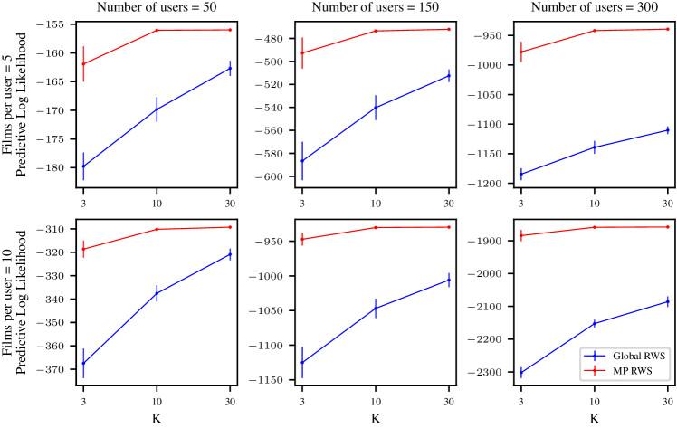
Figure 1: Results of massively parallel RWS and standard or “global” RWS for a hierarchical model on subsets of MovieLens with differing numbers of users and films per user, showing the predictive log likelihood after 25k training iterations.

These previous approaches draw $K$ samples from the full joint latent space. However, the required number of samples scales exponentially in the number of latent variables [Chatterjee and Diaconis, 2018]. Thus, we define a massively parallel scheme in which we draw $K$ samples for each latent variable, then effectively obtain $K^{n}$ samples by considering all combinations of $K$ samples for each of the $n$ latent variables. To that end, we denote each of the separate samples for separate latent variables $z_{i}^{k}\in\mathcal{Z}_{i}$, where $k$ indexes the sample and $i$ indexes the latent variable. We can write the collection of $K$ samples for a single latent variable (the $i$th) as,

$$z_{i} =(z_{i}^{1},z_{i}^{2},\dotsc,z_{i}^{K})\in\mathcal{Z}_{i}^{K}.$$ (9)

To sample all $K$ copies of the full joint latent space, TMC [Aitchison, 2019] uses an IID distribution over the $K$ samples, $z_{i}^{1},\dotsc,z_{i}^{K}$,

$${\operatorname{Q}}_{\textrm{TMC}}\left(z\middle|x\right) =\prod_{i=1}^{n}\prod_{k\in\mathcal{K}}{\operatorname{Q}}_{\textrm{TMC}}\left(z_{i}^{k}\middle|z_{j}\text{ for all }j\in{\textrm{qa}\left(i\right)}\right).$$ (10)

Here, ${\textrm{qa}\left(i\right)}$ are the indices of parents of the $i$th latent variable under the approximate posterior. In contrast, massively parallel methods allow for dependencies between the $K$ samples for the $i$th latent variable, $z_{i}^{1},\dotsc,z_{i}^{K}$ (Appendix B),

$${\operatorname{Q}}_{\textrm{MP}}\left(z\middle|x\right) =\prod_{i=1}^{n}{\operatorname{Q}}_{\textrm{MP}}\left(z_{i}\middle|z_{j}\text{ for all }j\in{\textrm{qa}\left(i\right)}\right).$$ (11)

There are no formal constraints on these dependencies. However, there are practical constraints, namely that we need to be able to efficiently compute the single-particle marginals, ${\operatorname{Q}}\left(z_{i}^{k}\middle|z_{j}\text{ for all }j\in{\textrm{qa}\left(i\right)}\right)$. In Appendix B, we give more specifics about choices of ${\operatorname{Q}}_{\textrm{MP}}\left(z_{i}\middle|z_{j}\text{ for all }j\in{\textrm{qa}\left(i\right)}\right)$ and ${\operatorname{Q}}_{\textrm{TMC}}\left(z_{i}^{k}\middle|z_{j}\text{ for all }j\in{\textrm{qa}\left(i\right)}\right)$. At a high level, these distributions are constructed by mixing the underlying single-sample approximate posterior, ${\operatorname{Q}}_{\phi}$, for different combinations of parent particles.

The generative model is more complicated, because we want to evaluate the generative probability for any of the $K^{n}$ possible combinations of the $K$ samples of the $n$ latent variables. To facilitate writing down these generative probabilities, we begin by defining a vector of indices,

$$\mathbf{k} =\left(k_{1},k_{2},\dotsc,k_{n}\right)\in\mathcal{K}^{n},$$ (12)

which has one index, $k_{i}$, for each of the $n$ latent variables. The latent variables specified by these indices is known as the “indexed” latent variables and can be written,

$$z^{\mathbf{k}} =\left(z_{1}^{k_{1}},z_{2}^{k_{2}},\dotsc,z_{n}^{k_{n}}\right)\in\mathcal{Z}.$$ (13)

The generative probability can thus be written,

$$\operatorname{P}_{\theta}\left(x,z^{\mathbf{k}}\right)= \operatorname{P}_{\theta}\left(x\middle|z_{j}^{k_{j}}\text{ for all }j\in{\textrm{pa}\left(x\right)}\right)$$ (14)

$$\prod_{i=1}^{n}\operatorname{P}_{\theta}\left(z^{k_{i}}_{i}\middle|z_{j}^{k_{j}}\text{ for all }j\in{\textrm{pa}\left(i\right)}\right).$$

Here, ${\textrm{pa}\left(i\right)}$ are the indices of parents of the $i$th latent variable under the generative model, and ${\textrm{pa}\left(x\right)}$ are the parents of the data under the generative model. Our use of ${\textrm{pa}\left(i\right)}$ mirrors our use of ${\textrm{qa}\left(i\right)}$ to denote indices of parents of the $i$th latent variable under the approximate posterior. Of course, the structure of the generative model and approximate posterior may differ, so ${\textrm{qa}\left(i\right)}$ and ${\textrm{pa}\left(i\right)}$ can also differ.

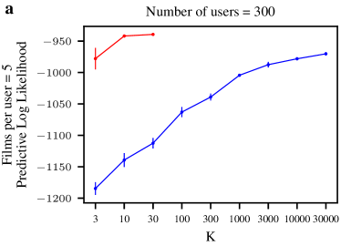
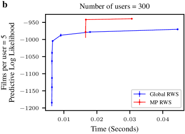
Figure 2: Comparison of performance between massively parallel RWS and global RWS, for the movielens dataset. a Same as Fig. 1 (top right), except that we use much higher values of $K$ for global RWS. b As massively parallel RWS may take longer than global RWS for a given $K$, we plotted time for a single training iteration against the predictive log-likelihood.

Looking at $\mathcal{P}_{\textrm{global}}(z)$ (Eq. 4) we average only over $K$ terms, corresponding to our $K$ samples from the full joint latent space. Our key contribution is to adapt RWS for the case where we average over all $K^{n}$ combinations of samples for each latent variable, indexed $\mathbf{k}$.

We can define an alternative unbiased marginal likelihood estimator, $\mathcal{P}_{\textrm{MP}}(z)$. This estimator is obtained by averaging over all $K^{n}$ combinations of all samples of all latent variables,

$$\mathcal{P}_{\textrm{MP}}(z) =\frac{1}{K^{n}}\sum_{\mathbf{k}\in\mathcal{K}^{n}}r_{\mathbf{k}}(z),$$ (15)

$$r_{\mathbf{k}}(z) =\frac{\operatorname{P}\left(x,z^{\mathbf{k}}\right)}{\prod_{i}{\operatorname{Q}}_{\textrm{MP}}\left(z_{i}^{k_{i}}\middle|z_{j}\text{ for all }j\in{\textrm{qa}\left(i\right)}\right)}$$ (16)

For the proof that $\mathcal{P}_{\textrm{MP}}(z)$ is an unbiased marginal likelihood estimator, see Appendix C.1.3. By analogy with global IWAE, we can define an objective for massively parallel IWAE,

$$\mathcal{L}_{\textrm{MP}} =\mathrm{E}_{{\operatorname{Q}}_{\textrm{MP}}\left(z\middle|x\right)}\left[\log\mathcal{P}_{\textrm{MP}}(z)\right].$$ (17)

We prove that this quantity has the required properties (specifically, that it is a lower-bound on the log marginal likelihood) in Appendix C.1.3. This quantity is very similar to that given in [Aitchison, 2019], except that it allows for a slightly more general proposal, ${\operatorname{Q}}_{\textrm{MP}}$, which allows for dependencies between the $K$ samples for a single latent variable, $z_{i}^{1},\dotsc,z_{i}^{K}$. Our key contribution is to design massively parallel updates for RWS,

$$\Delta\theta_{\textrm{MP}} {=}\mathrm{E}_{{\operatorname{Q}}_{\textrm{MP}}\left(z\middle|x\right)}\left[\frac{1}{K^{n}}\sum_{\mathbf{k}\in\mathcal{K}^{n}}\frac{r_{\mathbf{k}}(z)}{\mathcal{P}_{\textrm{MP}}(z)}\nabla_{\theta}\log\operatorname{P}_{\theta}\left(z^{\mathbf{k}},x\right)\right]$$ (18a)

$$\Delta\phi_{\textrm{MP}} {=}\mathrm{E}_{{\operatorname{Q}}_{\textrm{MP}}\left(z\middle|x\right)}\left[\frac{1}{K^{n}}\sum_{\mathbf{k}\in\mathcal{K}^{n}}\frac{r_{\mathbf{k}}(z)}{\mathcal{P}_{\textrm{MP}}(z)}\nabla_{\phi}\log{\operatorname{Q}}_{\phi}\left(z^{\mathbf{k}},x\right)\right]$$ (18b)

These updates are derived in Appendix C.2.2, and they can be implemented using,

$$\Delta\theta_{\textrm{MP}} =\mathrm{E}_{{\operatorname{Q}}_{\textrm{MP}}\left(z\middle|x\right)}\left[\nabla_{\theta}\log\mathcal{P}_{\textrm{MP}}(z)\right],$$ (19a)

$$\Delta\phi_{\textrm{MP}} =\mathrm{E}_{{\operatorname{Q}}_{\textrm{MP}}\left(z\middle|x\right)}\left[\nabla_{\phi}\left(-\log\mathcal{P}_{\textrm{MP}}(z)\right)\right],$$ (19b)

(see Appendix C.2.1).

Algorithm 1 Massively Parallel RWS

Data $x$, Prior $\mathrm{P}_{\theta}$, Proposal $\mathrm{Q}_{\mathrm{MP}}$, $K\geq 1$

for $i\leftarrow 1$ to $n$ do

     Sample $z_{i}\sim{\operatorname{Q}}_{\textrm{MP}}\left(z_{i}\middle|z_{j}\text{ for all }j\in{\textrm{qa}\left(i\right)}\right)$

     $z\leftarrow\{z_{1},...,z_{i-1}\}\cup z_{i}$

     $f^{i}_{k_{i},\mathbf{k}_{{\textrm{pa}\left(i\right)}}}(z)\leftarrow\frac{\operatorname{P}_{\theta}\left(z^{k_{i}}_{i}\middle|z_{j}^{k_{j}}\text{ for all }j\in{\textrm{pa}\left(i\right)}\right)}{{\operatorname{Q}}_{\textrm{MP}}\left(z_{i}^{k_{i}}|x,z_{j}\text{ for all }j\in{\textrm{qa}\left(i\right)}\right)}$

end for

$f^{x}_{\mathbf{k}_{{\textrm{pa}\left(x\right)}}}(z)\leftarrow\operatorname{P}_{\theta}\left(x\middle|z_{j}^{k_{j}}\text{ for all }j\in{\textrm{pa}\left(x\right)}\right)$

$\mathcal{P}_{\textrm{MP}}(z)\leftarrow\tfrac{1}{K^{n}}\sum_{\mathbf{k}^{n}}f^{x}_{\mathbf{k}_{{\textrm{pa}\left(x\right)}}}(z)\prod_{i}f^{i}_{k_{i},\mathbf{k}_{{\textrm{pa}\left(i\right)}}}(z)$

$\Delta\theta_{\textrm{MP}}\leftarrow{\nabla_{\theta}\log\mathcal{P}_{\textrm{MP}}(z)}$

$\Delta\phi_{\textrm{MP}}\leftarrow{\nabla_{\phi}\left(-\log\mathcal{P}_{\textrm{MP}}(z)\right)}$

4.1 Efficiently averaging exponentially many terms

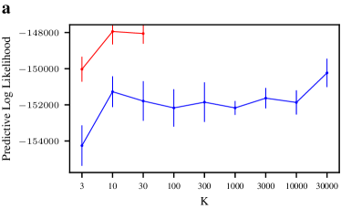
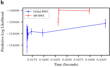
Figure 3: Comparison of performance for massively parallel RWS and global RWS on the NYC bus breakdown dataset. a Predictive log-likelihood against $K$ after 75k training iterations. b Predictive log-likelihood against the time for a single training iteration.

It should be surprising that we can compute $\mathcal{P}_{\textrm{MP}}(z)$ (Eq. 15) efficiently, as it involves summing over exponentially many ($K^{n}$) terms. However, it turns out that efficient computation is possible if we exploit structure in the generative model. To exploit structure, we first need to write down the generative probability for the $\mathbf{k}$th sample of all latent variables, $z^{\mathbf{k}}$. This looks alot like Eq. (14), as it follows the same graphical model structure, with ${\textrm{pa}\left(x\right)}$ and ${\textrm{pa}\left(i\right)}$ giving the indices of parents of the data and the $i$th latent variable respectively,

$$r_{\mathbf{k}}(z)= \operatorname{P}_{\theta}\left(x\middle|z_{j}^{k_{j}}\text{ for all }j\in{\textrm{pa}\left(x\right)}\right)$$ (20)

$$\prod_{i=1}^{n}\frac{\operatorname{P}_{\theta}\left(z^{k_{i}}_{i}\middle|z_{j}^{k_{j}}\text{ for all }j\in{\textrm{pa}\left(i\right)}\right).}{{\operatorname{Q}}_{\textrm{MP}}\left(z_{i}^{k_{i}}|x,z_{j}\text{ for all }j\in{\textrm{qa}\left(i\right)}\right)}$$

If we fix $z$ (i.e. all $K^{n}$ samples of all $n$ latent variables), then $r_{\mathbf{k}}(z)$ can be regarded as a big tensor with $K^{n}$ elements, indexed by $\mathbf{k}$. In that case, each term in the product defining $r_{\mathbf{k}}(z)$ (Eq. 20) can also be regarded as a tensor. The key observation is that the individual tensors in the product typically have only a few indices. For instance, the probability of the data, $x$, depends only on the indices of samples of the parents (i.e. $(k_{j}\text{ for all }j\in{\textrm{pa}\left(x\right)})$). These indices of the samples of the parents can be written,

$$\mathbf{k}_{{\textrm{pa}\left(x\right)}} =\left(k_{j}\text{ for all }j\in{\textrm{pa}\left(x\right)}\right)\in\mathcal{K}^{\left\lvert{\textrm{pa}\left(x\right)}\right\rvert},$$ (21a)

$$\mathbf{k}_{{\textrm{pa}\left(i\right)}} =\left(k_{j}\text{ for all }j\in{\textrm{pa}\left(i\right)}\right)\in\mathcal{K}^{\left\lvert{\textrm{pa}\left(i\right)}\right\rvert}.$$ (21b)

and where $\left\lvert{\textrm{pa}\left(x\right)}\right\rvert$ and $\left\lvert{\textrm{pa}\left(i\right)}\right\rvert$ are the number of parents latent variables. To make explicit the idea that the individual terms in Eq. (20) can be understood as tensors, we define $f^{x}_{\mathbf{k}_{{\textrm{pa}\left(x\right)}}}(z)$ as the tensor for the data and $f^{i}_{k_{i},\mathbf{k}_{{\textrm{pa}\left(i\right)}}}(z)$ as the tensor for the $i$th latent variable,

$$f^{x}_{\mathbf{k}_{{\textrm{pa}\left(x\right)}}}(z) =\operatorname{P}_{\theta}\left(x\middle|z_{j}^{k_{j}}\text{ for all }j\in{\textrm{pa}\left(x\right)}\right),$$ (22a)

$$f^{i}_{k_{i},\mathbf{k}_{{\textrm{pa}\left(i\right)}}}(z) =\frac{\operatorname{P}_{\theta}\left(z^{k_{i}}_{i}\middle|z_{j}^{k_{j}}\text{ for all }j\in{\textrm{pa}\left(i\right)}\right)}{{\operatorname{Q}}_{\textrm{MP}}\left(z_{i}^{k_{i}}|x,z_{j}\text{ for all }j\in{\textrm{qa}\left(i\right)}\right)}.$$ (22b)

Thus, we can write $r_{\mathbf{k}}(z)$ as a product of these factors,

$$r_{\mathbf{k}}(z) =f^{x}_{\mathbf{k}_{{\textrm{pa}\left(x\right)}}}(z)\prod_{i}f^{i}_{k_{i},\mathbf{k}_{{\textrm{pa}\left(i\right)}}}(z),$$ (23)

and $\mathcal{P}_{\textrm{MP}}(z)$ can be understood as a big tensor product,

$$\mathcal{P}_{\textrm{MP}}(z) =\tfrac{1}{K^{n}}\sum_{\mathbf{k}^{n}}f^{x}_{\mathbf{k}_{{\textrm{pa}\left(x\right)}}}(z)\prod_{i}f^{i}_{k_{i},\mathbf{k}_{{\textrm{pa}\left(i\right)}}}(z).$$ (24)

This tensor product can be efficiently computed in polynomial time by ordering the sums and products using Python packages such as opt-einsum [Daniel et al., 2018].

5 Experiments

We present an empirical evaluation of massively parallel RWS. Since the RWS wake phase ${\operatorname{Q}}$ requires multiple importance samples we test massively parallel RWS (MP RWS) with $K\in\{3,10,30\}$ and global RWS with $K\in\{3,10,30,100,300,1000,3000,10000,30000\}$. Unless otherwise stated our variational posterior is of the form $q_{\phi}(\mathbf{z})=\prod_{i=1}^{L}q(z_{i})$, where $q(z_{i})$ is from the same family of distributions as $z_{i}$’s distribution in the generative model. We compare massively parallel RWS (Eq. 18 and Eq. 19) and against standard “global” RWS (Eq. 7 and Eq. 8).

Optimisation is done using Adam [Kingma and Ba, 2014] with $\beta=(0.9,0.999)$, no weight decay, and a learning rate of $0.001$ which is decreased by a factor of $10$ every $10$k iterations. In all cases we plot the result of 5 runs with different random seeds and plot the mean and standard error. All times are measured on a single Nvidia A100 GPU.

5.1 Movielens dataset

We show results on the MovieLens100K dataset [Harper and Konstan, 2015]. This dataset consists of 100K ratings from $\mathrm{M}=943$ users (indexed $m$) of $\mathrm{N}=1682$ films (indexed $j$). Each film, indexed $j$, has as a feature vector $\mathbf{x}_{j}$. We observe user ratings, and following [Geffner and Domke, 2022], binarise ratings of $(0,1,2,3)$ to $0$ and ratings of $(4,5)$ to $1$. We use the following hierarchical model:

$$\boldsymbol{\mu} \sim\mathcal{N}(\mathbf{0}_{18},1)$$

$$\psi \sim\operatorname{Categorical}([0.1,0.5,0.4,0.05,0.05])$$

$$\mathbf{z}_{m} \sim\mathcal{N}(\boldsymbol{\mu},\exp(\psi)\mathbf{I}),\ m=1,\dotsc,M$$

$$\mathrm{Rating}_{mj} \sim\operatorname{Bernoulli}(\sigma(\mathbf{z}_{m}^{\intercal}\mathbf{x}_{j})),\ j=1,\dotsc,\mathrm{N}$$ (25)

This model, first samples a global mean, $\boldsymbol{\mu}$, and a discrete variance, $\psi$. We then sample a vector, $\mathbf{z}_{m}$ for each user, which describes the types of films that they will rate highly. The probability of a high rating is then given by taking the dot-product of the latent user-vector, $\mathbf{z}_{m}$ and the film’s feature vector, $\mathbf{x}_{j}$. A corresponding graphical model can be seen in Appendix C.3.

Note that this model has a discrete latent variable $\psi$. As RWS does not reparameterise gradients of the ELBO, inference can proceed straightforwardly, without needing any approaches to discrete latent variables from VI, such as summing out the latent variable, applying REINFORCE gradient estimators or using continuous relaxations [Le et al., 2020]. We compare the two methods by calculating the predictive log likelihood on a test set the same size as the training set.

To evaluate inference methods effectively, it is important to ensure that the posterior distributions are broad, and have not collapsed to very narrow point-like distributions. As such, we evaluate on subsets of the full MovieLens dataset, composed of either 5 or 10 films per user, and 50, 150 or 300 users.

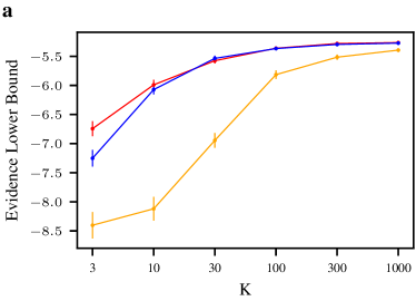
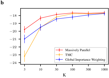
Figure 4: Comparison of performance between massively parallel methods, TMC, particle filter and global importance weighting. a The timeseries model with one observation. b The timeseries model with multiple observations.

Results are shown in Fig. 1 and Fig. 2. massively parallel RWS gives considerably higher predictive log-likelihoods for all $K$ (Fig. 1, 2a). Importantly, the massively parallel RWS updates are more complex than the global RWS updates, so may take longer. We therefore also considered the performance, measured as the predictive log-likelihood, against the time for a single training iteration. We again found considerable, albeit less dramatic, improvements (Fig. 2b).

5.2 NYC Bus breakdown dataset

The city of New York releases data on the length of delays to school bus journeys [DOE, 2023]. We model the length of the delay in terms of the type of journey, the school year in which the delay occurred, the borough the delay occurred in and the ID of the bus that was delayed.

To model delay time we use the model outlined in Appendix C.4. Because the dataset can be stratified into a hierarchy with three levels (Year, Borough and ID) we want our model to reflect this and, inspired by attempts to use hierarchical regression to model radon levels indoor radon levels [Price et al., 1996], we use a similar multi-level regression with three levels. This model first samples a variance and mean for each year, then uses these to sample a borough mean for each year. A variance is then sampled for each borough, which together with the year level borough mean is used to sample an ID mean for each year and borough. Finally, a variance is sampled and used to sample two weight vectors, $\mathbf{C}_{i}$ which has length “Number of bus companies” and $\mathbf{J}_{i}$ which has length “Number of types of journeys”. These are used to weight covariates that indicate which bus company was running a given ID’s route and which type of journey was being undertaken respectively. These are then summed with the sampled ID mean for that year and borough to get the logits for a negative binomial distribution that then gives the predicted delay for the $i$-th ID in the $j$-th borough in the $m$-th year. A corresponding graphical model can be seen in Appendix C.5.

We evaluate this model using a training dataset with $270$ observations: $I=30$ Ids from $J=3$ Boroughs in $M=3$ Years. We perform RWS for $75$k iterations, and evaluate the predictive log likelihood on a held out test set the same size as the training set.

Results are shown in Fig. 3. Again we see that massively parallel RWS outperforms global RWS for all $K$.

5.3 Comparing MP VI with TMC

Even though our main contribution is in developing massively parallel RWS, our derivations also allow for slightly more general massively parallel approaches to VI. In particular, our derivations allow us to couple the proposal for the $K$ samples of the $i$th latent variable, $z_{i}^{1},\dotsc,z_{i}^{K}$, while TMC [Aitchison, 2019] forces these $K$ samples to be IID. This coupling in massively parallel methods allows us to introduce variance-reduction strategies inspired by methods for reducing particle degeneracy in particle filters [Carpenter et al., 1999, Li et al., 2012, 2014, Zhou et al., 2016, Wang et al., 2017] (see Appendix B for further details).

To highlight these advantages, we considered two toy timeseries models: a single observation and a multi- observation model.

5.3.1 Single Observation

In the single observation model, there is a latent timeseries $z_{1},\dotsc,z_{30}$ (we use $N=30$), and an observation, $x$, only at the last timestep,

$$z_{1} =0,$$ (26)

$$z_{i} \sim\mathcal{N}(z_{i-1},1/N),$$

$$x \sim\mathcal{N}(z_{N},1)$$

We use the prior to define the proposal (see Appendix B). Results can be seen in figure 4a. For large $K$, all methods converge to the same value, as the ELBOs are all bounded by the true model evidence. To compare the methods, we therefore need to consider their relative performance for smaller values of $K$. We can see that the TMC (orange) [Aitchison, 2019] performs considerably worse than massively parallel VI (red) and IWAE (blue) [Burda et al., 2015]. We believe that TMC is performing poorly because of particle degeneracy [Carpenter et al., 1999, Li et al., 2012, 2014, Zhou et al., 2016, Wang et al., 2017]. In particular, the TMC proposal for $z_{i}$ is given by a mixture of the prior, conditioned particles from the previous timestep, $z_{i-1}$. In sampling from this mixture, in essence, we first sample a parent particle, $z_{i-1}^{k_{i-1}}$, then we sample from the prior, conditioned on that parent sample, $\operatorname{P}\left(z_{i}^{k_{i}}|z_{i-1}^{k_{i-1}}\right)$. In TMC, we choose these parent sample IID, which means that one parent particle, $z_{i-1}^{k_{i-1}}$ may have zero, one or multiple children. This is problematic: whenever a parent sample has zero children, then this reduces diversity in the samples of $z_{i}$, and this issue builds up over timesteps. Massively parallel methods circumvent this issue by ensuring that each parent sample has one and only one child sample (which requires us to couple the distribution over $z_{i}^{1},\dotsc,z_{i}^{K}$), and IWAE avoids the issue by simply sampling $z_{i}^{k}$ conditioned on $z_{i-1}^{k}$. Massively parallel is comparable to IWAE in this setting due to conditioning only a single scalar value at the end of the timeseries. These methods separate when we consider multiple observations (next).

5.3.2 Multiple Observations

Next, we considered a more standard timeseries with multiple observations. We are implementing these methods in the context of a new probabilistic programming language. This language currently has limitations on the number of latent variables that are inherited from the opt-einsum implementation. As such, we were not able to do the obvious thing of having one observation at every timestep. Instead, we had an observation every third timestep.

$$z_{1} \sim\mathcal{N}(0,1),$$ (27)

$$z_{i} \sim\mathcal{N}((1-\tfrac{1}{\tau})z_{i-1},2/\tau),$$

$$x_{i} \sim\mathcal{N}(z_{i},1)\quad\quad\text{if $i$ divisible by 3}.$$

Again, we use $N=30$. Results can be seen in Fig. 4. Again, the methods converge as $K$ increases, but this time, massively parallel VI (red) gives better performance than both alternatives for lower values of $K$.

6 Conclusion

We introduced massively parallel RWS, in which we draw $K$ samples for $n$ latent variables, and efficiently consider all $K^{n}$ combinations by exploiting conditional independencies in the generative model. We showed that massively parallel RWS represents a considerable improvement over previous RWS methods that draw $K$ samples from the full joint latent space.

Massively Parallel Reweighted Wake-Sleep (Supplementary Material)

Appendix A Proof of equivalence of the different forms of the global RWS updates

We start with the RWS $\operatorname{P}$ update (Eq. 8a), then use $\nabla_{\theta}\log\mathcal{P}_{\text{global}}(z)=\left(\nabla_{\theta}\mathcal{P}_{\text{global}}(z)\right)/\mathcal{P}_{\text{global}}(z)$,

$$\mathrm{E}\left[\Delta\theta_{\text{RWS}}\right] =\mathrm{E}_{{\operatorname{Q}}_{\phi}\left(z|x\right)}\left[\frac{\nabla_{\theta}\mathcal{P}_{\text{global}}(z)}{\mathcal{P}_{\textrm{global}}(z)}\right].$$ (28)

Using the definition of $$\mathcal{P}_{\text{global}}(z)$$ (Eq. 4),

$$\mathrm{E}\left[\Delta\theta_{\text{RWS}}\right] =\mathrm{E}_{{\operatorname{Q}}_{\phi}\left(z|x\right)}\left[\frac{\nabla_{\theta}\tfrac{1}{K}\sum_{k}r_{k}(z)}{\mathcal{P}_{\textrm{global}}(z)}\right]$$ (29)

Substituting for $$r_{k}(z)$$ (Eq. 5) in the numerator,

$$\mathrm{E}\left[\Delta\theta_{\text{RWS}}\right] =\mathrm{E}_{{\operatorname{Q}}_{\phi}\left(z|x\right)}\left[\frac{\tfrac{1}{K}\sum_{k}\frac{\nabla_{\theta}\operatorname{P}_{\theta}\left(z^{k},x\right)}{{\operatorname{Q}}_{\phi}\left(z^{k}|x\right)}}{\mathcal{P}_{\textrm{global}}(z)}\right]$$ (30)

substituting $$\nabla_{\theta}\operatorname{P}_{\theta}\left(z^{k},x\right)=\operatorname{P}_{\theta}\left(z^{k},x\right)\nabla_{\theta}\log\operatorname{P}_{\theta}\left(z^{k},x\right)$$,

$$\mathrm{E}\left[\Delta\theta_{\text{RWS}}\right] =\mathrm{E}_{{\operatorname{Q}}_{\phi}\left(z|x\right)}\left[\frac{1}{K}\sum_{k}\frac{\frac{\operatorname{P}_{\theta}\left(z^{k},x\right)}{{\operatorname{Q}}_{\phi}\left(z^{k}|x\right)}}{\mathcal{P}_{\textrm{global}}(z)}\nabla_{\theta}\log\operatorname{P}_{\theta}\left(z^{k},x\right)\right]$$ (31)

Noticing that the ratio of $\operatorname{P}_{\theta}\left(z^{k},x\right)$ and ${\operatorname{Q}}_{\phi}\left(z^{k}|x\right)$ in the numerator is equal to $r_{k}(z)$ (Eq. 5), we get back to Eq. (7a), as required.

The RWS ${\operatorname{Q}}$ update is very similar. Again, we start with Eq. (8b), then use $\nabla_{\theta}\log\mathcal{P}_{\text{global}}(z)=\left(\nabla_{\theta}\mathcal{P}_{\text{global}}(z)\right)/\mathcal{P}_{\text{global}}(z)$,

$$\mathrm{E}\left[\Delta\phi_{\text{RWS}}\right] =-\mathrm{E}_{{\operatorname{Q}}_{\phi}\left(z|x\right)}\left[\frac{\nabla_{\phi}\mathcal{P}_{\text{global}}(z)}{\mathcal{P}_{\text{global}}(z)}\right]$$ (32)

Using the definition of $$\mathcal{P}_{\text{global}}(z)$$ (Eq. 4),

$$\mathrm{E}\left[\Delta\phi_{\text{RWS}}\right] =-\mathrm{E}_{{\operatorname{Q}}_{\phi}\left(z|x\right)}\left[\frac{\nabla_{\phi}\tfrac{1}{K}\sum_{k}r_{k}(z)}{\mathcal{P}_{\textrm{global}}(z)}\right]$$ (33)

Substituting for $$r_{k}(z)$$ (Eq. 5) in the numerator,

$$\mathrm{E}\left[\Delta\phi_{\text{RWS}}\right] =-\mathrm{E}_{{\operatorname{Q}}_{\phi}\left(z|x\right)}\left[\frac{\tfrac{1}{K}\sum_{k}\nabla_{\phi}\frac{\operatorname{P}_{\theta}\left(z^{k},x\right)}{{\operatorname{Q}}_{\phi}\left(z^{k}|x\right)}}{\mathcal{P}_{\textrm{global}}(z)}\right]$$ (34)

Computing the derivative,

$$\mathrm{E}\left[\Delta\phi_{\text{RWS}}\right] =\mathrm{E}_{{\operatorname{Q}}_{\phi}\left(z|x\right)}\left[\frac{\tfrac{1}{K}\sum_{k}\frac{\operatorname{P}_{\theta}\left(z^{k},x\right)}{\left({\operatorname{Q}}_{\phi}\left(z^{k}|x\right)\right)^{2}}\nabla_{\phi}{\operatorname{Q}}_{\phi}\left(z^{k}|x\right)}{\mathcal{P}_{\textrm{global}}(z)}\right].$$ (35)

Noticing that $$\left(\nabla_{\phi}{\operatorname{Q}}_{\phi}\left(z^{k}|x\right)\right)/{\operatorname{Q}}_{\phi}\left(z^{k}|x\right)=\nabla_{\phi}\log{\operatorname{Q}}_{\phi}\left(z^{k}|x\right)$$,

$$\mathrm{E}\left[\Delta\phi_{\text{RWS}}\right] =\mathrm{E}_{{\operatorname{Q}}_{\phi}\left(z|x\right)}\left[\frac{\tfrac{1}{K}\sum_{k}\frac{\operatorname{P}_{\theta}\left(z^{k},x\right)}{{\operatorname{Q}}_{\phi}\left(z^{k}|x\right)}\nabla_{\phi}\log{\operatorname{Q}}_{\phi}\left(z^{k}|x\right)}{\mathcal{P}_{\textrm{global}}(z)}\right].$$ (36)

Finally, noticing that the ratio of $\operatorname{P}_{\theta}\left(z^{k},x\right)$ and ${\operatorname{Q}}_{\phi}\left(z^{k}|x\right)$ in the numerator is equal to $r_{k}(z)$ (Eq. 5), we get back to Eq. (7b), as required.

Both of these derivations may be straightforwardly repeated for the massively parallel setting, simply by replacing $k\in\mathcal{K}$ with $\mathbf{k}\in\mathcal{K}^{n}$, and by replacing $1/K$ with $1/K^{n}$.

Appendix B TMC vs massively parallel approximate posteriors

TMC approximate posteriors draw the $K$ samples of the $i$th latent variable IID,

$${\operatorname{Q}}_{\textrm{TMC}}\left(z_{i}\middle|z_{j}\text{ for all }j\in{\textrm{qa}\left(i\right)}\right) =\prod_{k_{i}\in\mathcal{K}}{\operatorname{Q}}_{\textrm{TMC}}\left(z_{i}^{k_{i}}\middle|z_{j}\text{ for all }j\in{\textrm{qa}\left(i\right)}\right)$$ (37)

Specifically, TMC draws each sample from an equally weighted mixture over all parent particles,

$${\operatorname{Q}}_{\textrm{TMC}}\left(z_{i}^{k_{i}}\middle|z_{j}\text{ for all }j\in{\textrm{qa}\left(i\right)}\right) =\tfrac{1}{K^{|{\textrm{qa}\left(i\right)}|}}\sum_{\mathbf{k}_{{\textrm{qa}\left(i\right)}}}{\operatorname{Q}}_{\textrm{global}}\left(z_{i}^{k_{i}}\middle|z_{j}^{k_{j}}\text{ for all }j\in{\textrm{qa}\left(i\right)}\right).$$ (38)

In contrast, massively parallel methods do not force us to sample particles IID. The key issue with IID sampling is that it introduces the risk of particle degeneracy [Carpenter et al., 1999, Li et al., 2012, 2014, Zhou et al., 2016, Wang et al., 2017]. In particle degeneracy, some of the parent samples (e.g. $z_{j}^{1}$ where $j\in{\textrm{qa}\left(i\right)}$) might have multiple children, in the sense that multiple $z_{i}^{k}$ are sampled from the mixture component arising from $z_{j}^{1}$. At the same time, some of the parents, (e.g. $z_{j}^{2}$) might have no children, in the sense that no $z_{i}^{k}$ are sampled from a mixture component arising from $z_{j}^{2}$. This is problematic because it reduces diversity in the population of samples, $z_{i}=(z_{i}^{1},\dotsc,z_{i}^{K})$, and this reduction in diversity can be especially problematic in models with long chains of latent variables, such as timeseries models. To reduce the risk of particle degeneracy, the massively parallel methods considered here couple the distribution over each of the $K$ particles,

$${\operatorname{Q}}_{\textrm{MP}}\left(z_{i}\middle|z_{j}\text{ for all }j\in{\textrm{qa}\left(i\right)}\right) \neq\prod_{k_{i}\in\mathcal{K}}{\operatorname{Q}}_{\textrm{TMC}}\left(z_{i}^{k_{i}}\middle|z_{j}\text{ for all }j\in{\textrm{qa}\left(i\right)}\right).$$ (39)

However, we do ensure that the marginal for a single particle is the same as for TMC,

$${\operatorname{Q}}_{\textrm{MP}}\left(z_{i}^{k_{i}}\middle|z_{j}\text{ for all }j\in{\textrm{qa}\left(i\right)}\right) =\tfrac{1}{K^{|{\textrm{qa}\left(i\right)}|}}\sum_{\mathbf{k}_{{\textrm{qa}\left(i\right)}}}{\operatorname{Q}}_{\textrm{global}}\left(z_{i}^{k_{i}}\middle|z_{j}^{k_{j}}\text{ for all }j\in{\textrm{qa}\left(i\right)}\right).$$ (40)

To achieve this, we sample a permutation, $\pi$ for each latent variable, and the permutation tells us which parent particle to consider. To give an example for one parent,

$${\operatorname{Q}}_{\textrm{MP}}\left(z_{i}\middle|\pi,z_{j}\right) =\prod_{k_{i}}{\operatorname{Q}}_{\textrm{MP}}\left(z_{i}^{k_{i}}\middle|\pi,z_{j}\right)$$ (41)

$${\operatorname{Q}}_{\textrm{MP}}\left(z_{i}^{k_{i}}\middle|\pi,z_{j}\right) =\tfrac{1}{K}\sum_{k_{i}}{\operatorname{Q}}_{\phi}\left(z_{i}^{k_{i}}\middle|z_{j}^{\pi_{k_{i}}}\right)$$ (42)

Critically, if we marginalise over the permutation, the distribution over a single $z_{i}^{k_{i}}$ has the same density as that from a uniform mixture,

$${\operatorname{Q}}_{\textrm{MP}}\left(z_{i}^{k_{i}}\middle|z_{j}\right) =\sum_{\pi}{\operatorname{Q}}_{\textrm{MP}}\left(z_{i}^{k_{i}}\middle|\pi,z_{j}\right)$$ (43)

$${\operatorname{Q}}_{\textrm{MP}}\left(z_{i}^{k_{i}}\middle|z_{j}\right) =\tfrac{1}{K}\sum_{k_{j}}{\operatorname{Q}}_{\phi}\left(z_{i}^{k_{i}}\middle|z_{j}^{k_{j}}\right).$$ (44)

Finally, if we have multiple parent latent variables, we independently sample a permutation for each latent variable.

Appendix C Massively parallel IWAE and RWS

Before getting started, it will prove useful to define some briefer notation than that used in the main text. Specifically, we use,

$$z_{\textrm{qa}\left(i\right)} =\left\{z_{j}\text{ for all }j\in{\textrm{qa}\left(i\right)}\right\},$$ (45)

$$z^{k_{i}}_{\textrm{qa}\left(i\right)} =\left\{z_{j}^{k_{i}}\text{ for all }j\in{\textrm{qa}\left(i\right)}\right\},$$ (46)

$$z^{\mathbf{k}_{\textrm{pa}\left(i\right)}}_{\textrm{pa}\left(i\right)} =\left\{z_{j}^{k_{j}}\text{ for all }j\in{\textrm{pa}\left(i\right)}\right\},$$ (47)

so,

$${\operatorname{Q}}\left(z_{i}^{k_{i}}\middle|x,z_{\textrm{qa}\left(i\right)}\right) ={\operatorname{Q}}\left(z_{i}^{k_{i}}\middle|x,z_{j}\text{ for all }j\in{\textrm{qa}\left(i\right)}\right),$$ (48)

$$\operatorname{P}_{\theta}\left(z^{k_{i}}_{i}\middle|z^{\mathbf{k}_{\textrm{pa}\left(i\right)}}_{\textrm{pa}\left(i\right)}\right) =\operatorname{P}_{\theta}\left(z^{k_{i}}_{i}\middle|z_{j}^{k_{j}}\text{ for all }j\in{\textrm{pa}\left(i\right)}\right)$$ (49)

Note that in Eq. (48), we allow for the possibility of a slightly more general form for the approximate posterior, where the distribution over $z_{i}^{k_{i}}$ may depend on any of the parent samples. This generalisation ensures that the subsequent derivations generalise to other possible forms for the approximate posterior, such as those for TMC (Eq. 11).

In addition, it is useful to introduce notation to describe the “non-indexed” latent variables (i.e. everything in $z$ that is not $z^{\mathbf{k}}$). The $i$th non-indexed latents are, $z_{i}^{/\mathbf{k}_{i}}$,

$$z_{i}^{/k_{i}} =\left(z_{i}^{1},\dotsc,z_{i}^{k_{i}-1},z_{i}^{k_{i}+1},\dotsc,z_{i}^{K}\right)\in\mathcal{Z}_{i}^{K-1}.$$ (50)

and $$z^{/\mathbf{k}}$$ are all non-indexed latents,

$$z^{/\mathbf{k}} =\left(z_{1}^{/k_{1}},z_{2}^{/k_{2}},\dotsc,z_{n}^{/k_{n}}\right)\in\mathcal{Z}^{K-1}.$$ (51)

C.1 IWAE

C.1.1 Single-Sample VI

We begin by building intuition by looking at the derivation for the ELBO in the standard single-sample VAE. We start by writing the marginal likelihood as an integral,

$$\operatorname{P}_{\theta}\left(x\right) =\int dz^{\prime}\operatorname{P}_{\theta}\left(x,z^{\prime}\right).$$ (52)

Here, we use $$z^{\prime}\in\mathcal{Z} z^{\prime} z z K {\operatorname{Q}}_{\phi}\left(z^{\prime}|x\right)$$ to denote a single sample from the full joint state space; we use instead of because is reserved for samples (Eq. 2). Next, we divide and multiply by the approximate posterior probability, ,

$$\operatorname{P}_{\theta}\left(x\right) =\int dz^{\prime}{\operatorname{Q}}_{\phi}\left(z^{\prime}|x\right)\frac{\operatorname{P}_{\theta}\left(x,z^{\prime}\right)}{{\operatorname{Q}}_{\phi}\left(z^{\prime}|x\right)}.$$ (53)

Now, we can rewrite the integral as an expectation under the approximate posterior,

$$\operatorname{P}_{\theta}\left(x\right) =\mathrm{E}_{{\operatorname{Q}}_{\phi}\left(z^{\prime}|x\right)}\left[\frac{\operatorname{P}_{\theta}\left(x,z^{\prime}\right)}{{\operatorname{Q}}_{\phi}\left(z^{\prime}|x\right)}\right].$$ (54)

Now we take the logarithm on both sides and apply Jensen’s inequality,

$$\log\operatorname{P}_{\theta}\left(x\right) =\log\mathrm{E}_{{\operatorname{Q}}_{\phi}\left(z^{\prime}|x\right)}\left[\frac{\operatorname{P}_{\theta}\left(x,z^{\prime}\right)}{{\operatorname{Q}}_{\phi}\left(z^{\prime}|x\right)}\right]\geq\mathrm{E}_{{\operatorname{Q}}_{\phi}\left(z^{\prime}|x\right)}\left[\log\frac{\operatorname{P}_{\theta}\left(x,z^{\prime}\right)}{{\operatorname{Q}}_{\phi}\left(z^{\prime}|x\right)}\right]=\mathcal{L}_{\text{VAE}}$$ (55)

Of course, this derivation is specific to the single-sample VAE. But we can pull out an underlying strategy that generalises to the multi-sample setting. In particular, we first come up with an unbiased estimator of the marginal likelihood. In our VAE, this is,

$$\mathcal{P}_{\text{VAE}}(z^{\prime}) =\frac{\operatorname{P}_{\theta}\left(x,z^{\prime}\right)}{{\operatorname{Q}}_{\phi}\left(z^{\prime}|x\right)}$$ (56)

Following Eq. (54) we can see that this quantity is an unbiased estimator of the marginal likelihood if $$z^{\prime} {\operatorname{Q}}_{\phi}\left(z^{\prime}|x\right)$$ is sampled from ,

$$\operatorname{P}_{\theta}\left(x\right) =\mathrm{E}_{{\operatorname{Q}}_{\phi}\left(z^{\prime}|x\right)}\left[\mathcal{P}_{\text{VAE}}(z^{\prime})\right]$$ (57)

Then we apply Jensen’s inequality (Eq. 55),

$$\log\operatorname{P}_{\theta}\left(x\right) \geq\mathcal{L}_{\text{VAE}}=\mathrm{E}_{{\operatorname{Q}}_{\phi}\left(z^{\prime}|x\right)}\left[\log\mathcal{P}_{\text{VAE}}(z^{\prime})\right].$$ (58)

However, this approach highlights key issues with the usual single-sample bound. In particular, the single-sample estimator, $\mathcal{P}_{\text{VAE}}(z^{\prime})$ can be very high-variance, and variance in the unbiased estimator causes the Jensen bound to become looser.

C.1.2 Global IWAE

To reduce variance in the unbiased estimator, a natural approach is to average $K$ independent samples, and this is exactly what global IWAE does,

$$\mathcal{P}_{\textrm{global}}(z) =\frac{1}{K}\sum_{k=1}^{K}r_{k}(z)=\frac{1}{K}\sum_{k=1}^{K}\mathcal{P}_{\text{VAE}}(z^{k})$$ (59)

This is of course an unbiased estimator, as it is the average of $K$ unbiased estimators,

$$\operatorname{P}_{\theta}\left(x\right) =\mathrm{E}_{{\operatorname{Q}}_{\phi}\left(z|x\right)}\left[\mathcal{P}_{\textrm{global}}(z)\right].$$ (60)

Therefore, applying Jensen’s inequality gives a new lower-bound on the log-marginal likelihood,

$$\log\operatorname{P}_{\theta}\left(x\right) =\log\mathrm{E}_{{\operatorname{Q}}_{\phi}\left(z|x\right)}\left[\mathcal{P}_{\textrm{MP}}(z)\right]\geq\mathrm{E}_{{\operatorname{Q}}_{\phi}\left(z|x\right)}\left[\log\mathcal{P}_{\textrm{global}}(z)\right]=\mathcal{L}_{\text{IWAE}}$$ (61)

which is tighter than the usual single-sample ELBO [Burda et al., 2015], and which matches Eq. (6) in the main text.

C.1.3 Massively Parallel IWAE

Our proposed $\mathcal{P}_{\textrm{MP}}(z)$ (Eq. 15) is the average of $K^{n}$ terms, rather than $K$ terms in global IWAE. To prove that our massively parallel strategy is valid, our strategy is to show that every term in this average is an unbiased estimator of $\log\operatorname{P}_{\theta}\left(x\right)$, in which case the average is also an unbiased estimator, and we can again apply Jensen.

Each term in the average $\mathcal{P}_{\textrm{MP}}(z)$ (Eq. 15) is of the form $r_{\mathbf{k}}(z)$ (Eq. 16). The expectation of each term is,

$$\mathrm{E}_{{\operatorname{Q}}_{\phi}\left(z|x\right)}\left[r_{\mathbf{k}}(z)\right] =\mathrm{E}_{{\operatorname{Q}}_{\phi}\left(z|x\right)}\left[\frac{\operatorname{P}_{\theta}\left(x,z^{\mathbf{k}}\right)}{\prod_{i}{\operatorname{Q}}_{\phi}\left(z_{i}^{k_{i}}|x,z_{{\textrm{qa}\left(i\right)}}\right)}\right].$$ (62)

We can rewrite the expectation as an integral,

$$\mathrm{E}_{{\operatorname{Q}}_{\phi}\left(z|x\right)}\left[r_{\mathbf{k}}(z)\right] =\int dz\operatorname{P}_{\theta}\left(x,z^{\mathbf{k}}\right)\prod_{i}\frac{{\operatorname{Q}}_{\phi}\left(z_{i}|x,z_{{\textrm{qa}\left(i\right)}}\right)}{{\operatorname{Q}}_{\phi}\left(z_{i}^{k_{i}}|x,z_{{\textrm{qa}\left(i\right)}}\right)}.$$ (63)

Bayes theorem tells us,

$$\frac{{\operatorname{Q}}_{\phi}\left(z_{i}|x,z_{{\textrm{qa}\left(i\right)}}\right)}{{\operatorname{Q}}_{\phi}\left(z_{i}^{k_{i}}|x,z_{{\textrm{qa}\left(i\right)}}\right)} =\frac{{\operatorname{Q}}_{\phi}\left(z_{i}^{k_{i}},z_{i}^{/k_{i}}|x,z_{{\textrm{qa}\left(i\right)}}\right)}{{\operatorname{Q}}_{\phi}\left(z_{i}^{k_{i}}|x,z_{{\textrm{qa}\left(i\right)}}\right)}={\operatorname{Q}}\left(z_{i}^{/k_{i}}|x,z_{i}^{k_{i}},z_{{\textrm{qa}\left(i\right)}}\right),$$ (64)

Applying Bayes theorem,

$$\mathrm{E}_{{\operatorname{Q}}_{\phi}\left(z|x\right)}\left[r_{\mathbf{k}}(z)\right] =\int dz\operatorname{P}_{\theta}\left(x,z^{\mathbf{k}}\right)\prod_{i}{\operatorname{Q}}\left(z_{i}^{/k_{i}}|x,z_{i}^{k_{i}},z_{{\textrm{qa}\left(i\right)}}\right).$$ (65)

Importantly, the integrand is a valid joint distribution over $x$ and $z$, or equivalently over $x$, $z^{\mathbf{k}}$ and $z^{/\mathbf{k}}$. Thus, integrating over $z^{/\mathbf{k}}$ then $z^{\mathbf{k}}$, we find,

$$\mathrm{E}_{{\operatorname{Q}}_{\phi}\left(z|x\right)}\left[r_{\mathbf{k}}(z)\right] =\operatorname{P}_{\theta}\left(x\right).$$ (66)

As such, each of the $r_{\mathbf{k}}(z)$ terms is an unbiased estimator of the marginal likelihood. As $\mathcal{P}_{\textrm{MP}}(z)$ (Eq. 15) is just an average of $K^{n}$ $r_{\mathbf{k}}(z)$ terms, it is also an unbiased estimator. Applying Jensen’s inequality to this unbiased estimator,

$$\log\operatorname{P}_{\theta}\left(x\right) \geq\mathrm{E}_{{\operatorname{Q}}_{\phi}\left(z|x\right)}\left[\log\mathcal{P}_{\textrm{MP}}(z)\right]=\mathcal{L}_{\textrm{MP}},$$ (67)

which mirrors Eq. (17) in the main text.

C.2 RWS

C.2.1 Global RWS

To build intuition, we first give a derivation of the standard RWS updates. Ideally the updates would use samples drawn from the true posterior, $\operatorname{P}_{\theta}\left(z|x\right)$,

$$\Delta\theta_{\textrm{post}} =\mathrm{E}_{\operatorname{P}_{\theta}\left(z^{k}|x\right)}\left[\nabla_{\theta}\log\operatorname{P}_{\theta}\left(z,x\right)\right]$$ (68a)

$$\Delta\phi_{\textrm{post}} =\mathrm{E}_{\operatorname{P}_{\theta}\left(z^{k}|x\right)}\left[\nabla_{\phi}\log{\operatorname{Q}}_{\phi}\left(z|x\right)\right]$$ (68b)

The $\operatorname{P}$ update is exactly the M-step in EM, and the ${\operatorname{Q}}$ step trains ${\operatorname{Q}}_{\phi}\left(z|x\right)$ using maximum likelihood based on samples from the true posterior. To simplify the derivations, we note that both of these updates can be understood as computing a moment under the true posterior,

$$\Delta_{\textrm{post}} =\mathrm{E}_{\operatorname{P}_{\theta}\left(z^{k}|x\right)}\left[\Delta(z^{k})\right].$$ (69)

For the $\operatorname{P}$ update, we have $\Delta_{\textrm{post}}=\Delta\theta_{\textrm{post}}$ and $\Delta(z^{k})=\nabla_{\theta}\log\operatorname{P}_{\theta}\left(z,x\right)$. For the ${\operatorname{Q}}$ update, we have $\Delta_{\textrm{post}}=\Delta\phi_{\textrm{post}}$ and $\Delta(z^{k})=\nabla_{\theta}\log{\operatorname{Q}}_{\phi}\left(z,x\right)$. Of course, in practice, the true posterior is intractable, so instead we must use some form of importance weighting. We begin by writing the generic form for the updates as an integral,

$$\Delta_{\textrm{post}} =\int dz^{k}\operatorname{P}\left(z^{k}|x\right)\Delta(z^{k}).$$ (70)

We then multiply and divide by an approximate posterior, $${\operatorname{Q}}\left(z^{k}|x\right)$$,

$$\Delta_{\textrm{post}} =\int dz^{k}{\operatorname{Q}}\left(z^{k}|x\right)\frac{\operatorname{P}\left(z^{k}|x\right)}{{\operatorname{Q}}\left(z^{k}|x\right)}\Delta(z^{k}).$$ (71)

We can rewrite the integral as expectation over the approximate posterior, $${\operatorname{Q}}\left(z^{k}|x\right)$$,

$$\Delta_{\textrm{post}} =\mathrm{E}_{{\operatorname{Q}}\left(z^{k}|x\right)}\left[\frac{\operatorname{P}\left(z^{k}|x\right)}{{\operatorname{Q}}\left(z^{k}|x\right)}\Delta(z^{k})\right].$$ (72)

This quantity is difficult to use directly, because computing the posterior, $\operatorname{P}\left(z^{k}|x\right)$ involves the marginal likelihood, $\operatorname{P}_{\theta}\left(x\right)$, which is intractable,

$$\operatorname{P}_{\theta}\left(z^{k}|x\right) =\tfrac{\operatorname{P}_{\theta}\left(z^{k},x\right)}{\operatorname{P}_{\theta}\left(x\right)} \operatorname{P}_{\theta}\left(x\right)=\int dz^{k}\operatorname{P}_{\theta}\left(z^{k},x\right).$$ (73)

As the true marginal likelihood is intractable, we instead use $\mathcal{P}_{\textrm{global}}(z)$ (Eq. 4), which is an unbiased estimator of $\operatorname{P}\left(x\right)$, and is correct in the limit as $K\rightarrow\infty$ [Burda et al., 2015]. This gives updates of the form,

$$\Delta_{\textrm{global}} =\mathrm{E}_{{\operatorname{Q}}\left(z^{k}|x\right)}\left[\frac{\frac{\operatorname{P}\left(z^{k},x\right)}{{\operatorname{Q}}\left(z^{k}|x\right)}}{\mathcal{P}_{\textrm{global}}(z)}\Delta(z^{k})\right].$$ (74)

Remembering the definition of $r_{k}(z)$ (Eq. 5), this can be written,

$$\Delta_{\textrm{global}} =\mathrm{E}_{{\operatorname{Q}}_{\phi}\left(z|x\right)}\left[\frac{r_{k}(z)}{\mathcal{P}_{\textrm{global}}(z)}\Delta(z^{k})\right].$$ (75)

Finally as the expectation is the same for all $k$, we can average over $k$, which gives the expression in the main text (Eq. 7)

C.2.2 Massively Parallel RWS

Now, we can move on to massively parallel RWS. In the previous derivation for global RWS, we showed that each sample, $z^{k}$, individually constituted an unbiased estimator. In the massively parallel setting, the key difference is that instead of having $K$ samples $z^{k}$, we have $K^{n}$ samples, $z^{\mathbf{k}}$. In particular,

$$\Delta_{\textrm{post}} =\mathrm{E}_{\operatorname{P}\left(z^{\mathbf{k}}|x\right)}\left[\Delta(z^{\mathbf{k}})\right]=\int dz^{\mathbf{k}}\operatorname{P}\left(z^{\mathbf{k}}|x\right)\Delta(z^{\mathbf{k}}).$$ (76)

Now, we multiply and divide by $$\prod_{i}{\operatorname{Q}}\left(z_{i}^{k_{i}}\middle|x,z_{\textrm{qa}\left(i\right)}\right)$$,

$$\Delta_{\textrm{post}} =\int dz^{\mathbf{k}}\left(\prod_{i}{\operatorname{Q}}\left(z_{i}^{k_{i}}\middle|x,z_{\textrm{qa}\left(i\right)}\right)\right)\frac{\operatorname{P}\left(z^{\mathbf{k}}|x\right)}{\prod_{i}{\operatorname{Q}}\left(z_{i}^{k_{i}}\middle|x,z_{\textrm{qa}\left(i\right)}\right)}\Delta(z^{\mathbf{k}}).$$ (77)

Now, we introduce and integrate out a distribution over the non-indexed latent variables, $\prod_{i}{\operatorname{Q}}\left(z_{i}^{/k_{i}}\middle|x,z_{i}^{k_{i}},z_{\textrm{qa}\left(i\right)}\right)$

$$1 =\int dz^{/\mathbf{k}}\prod_{i}{\operatorname{Q}}\left(z_{i}^{/k_{i}}\middle|x,z_{i}^{k_{i}},z_{\textrm{qa}\left(i\right)}\right),$$ (78)

Multiplying Eq. (77) by $1$ (Eq. 78),

$$\Delta_{\textrm{post}} =\int dz^{\mathbf{k}}\left(\prod_{i}{\operatorname{Q}}\left(z_{i}^{k_{i}}\middle|x,z_{\textrm{qa}\left(i\right)}\right)\right)\frac{\operatorname{P}\left(z^{\mathbf{k}}|x\right)}{\prod_{i}{\operatorname{Q}}\left(z_{i}^{k_{i}}\middle|x,z_{\textrm{qa}\left(i\right)}\right)}\Delta(z^{\mathbf{k}})\int dz^{/\mathbf{k}}\prod_{i}{\operatorname{Q}}\left(z_{i}^{/k_{i}}\middle|x,z_{i}^{k_{i}},z_{\textrm{qa}\left(i\right)}\right).$$ (79)

Combining the integrals over $z^{\mathbf{k}}$ and $z^{/\mathbf{k}}$ into a single integral over $z$,

$$\Delta_{\textrm{post}} =\int dz{\operatorname{Q}}\left(z\middle|x\right)\frac{\operatorname{P}\left(z^{\mathbf{k}}|x\right)}{\prod_{i}{\operatorname{Q}}\left(z_{i}^{k_{i}}\middle|x,z_{\textrm{qa}\left(i\right)}\right)}\Delta(z^{\mathbf{k}}).$$ (80)

Writing the integral as an expectation,

$$\Delta_{\textrm{post}} =\mathrm{E}_{{\operatorname{Q}}_{\phi}\left(z|x\right)}\left[\frac{\operatorname{P}\left(z^{\mathbf{k}}|x\right)}{\prod_{i}{\operatorname{Q}}\left(z_{i}^{k_{i}}|x,z_{{\textrm{pa}\left(i\right)}}\right)}\Delta(z^{\mathbf{k}})\right].$$ (81)

Again, the posterior can be written,

$$\operatorname{P}_{\theta}\left(z^{\mathbf{k}}|x\right) =\tfrac{\operatorname{P}_{\theta}\left(z^{\mathbf{k}},x\right)}{\operatorname{P}_{\theta}\left(x\right)} \operatorname{P}_{\theta}\left(x\right)=\int dz^{\mathbf{k}}\operatorname{P}_{\theta}\left(z^{\mathbf{k}},x\right).$$ (82)

Again, the marginal likelihood, $\operatorname{P}_{\theta}\left(x\right)$ is intractable. Instead, we use the massively parallel estimate of the marginal likelihood, which was shown to be unbiased in Sec. C.1.3,

$$\Delta_{\textrm{MP}} =\mathrm{E}_{{\operatorname{Q}}_{\phi}\left(z|x\right)}\left[\frac{\frac{\operatorname{P}\left(z^{\mathbf{k}},x\right)}{\prod_{i}{\operatorname{Q}}\left(z_{i}^{k_{i}}|x,z_{{\textrm{pa}\left(i\right)}}\right)}}{\mathcal{P}_{\textrm{MP}}(z)}\Delta(z^{\mathbf{k}})\right].$$ (83)

Remembering the definition of $r_{\mathbf{k}}(z)$ (Eq. 16), this can be written,

$$\Delta_{\textrm{MP}} =\mathrm{E}_{{\operatorname{Q}}_{\phi}\left(z|x\right)}\left[\frac{r_{\mathbf{k}}(z)}{\mathcal{P}_{\textrm{MP}}(z)}\Delta(z^{\mathbf{k}})\right].$$ (84)

Finally, note that the expectation is the same for every value of $\mathbf{k}$. Averaging over all $K^{n}$ values of $\mathbf{k}$, we get the form in the main text (Eq. 18).

C.3 MovieLens Graphical Model

Figure 5: Graphical model for the MovieLens dataset

C.4 Bus Delay Model Specification

$$\begin{split}\mathrm{YearVariance}&\sim\mathrm{Cat}([0.1,0.5,0.4,0.05,0.05])\\ \mathrm{YearMean}&\sim\mathcal{N}(0,10^{-4})\\ \mathrm{BoroughMean}_{m}&\sim\mathcal{N}(\mathrm{YearMean},\exp(\mathrm{YearVariance})),\ m=1,...,\mathrm{M}\\ \mathrm{BoroughVariance}_{j}&\sim\mathrm{Cat}([0.1,0.4,0.05,0.5,0.05]),j=1,...,\mathrm{J}\\ \mathrm{IdMean}_{mj}&\sim\mathcal{N}(\mathrm{BoroughMean}_{m},\mathrm{BoroughVariance}_{j}),\ j=1,...,\mathrm{J},\ m=1,...,\mathrm{M}\\ \mathrm{WeightVariance}_{i}&\sim\mathrm{Cat}([0.1,0.4,0.5,0.05,0.05]),\ i=1,...,\mathrm{I}\\ \mathbf{C}_{i}&\sim\mathcal{N}(\mathbf{0}_{\#\mathrm{BusCo.s}},\mathrm{WeightVariance}_{i}),\ i=1,...,\mathrm{I}\\ \mathbf{J}_{i}&\sim\mathcal{N}(\mathbf{0}_{\#\mathrm{JourneyTypes}},\mathrm{WeightVariance}_{i}),\ i=1,...,\mathrm{I}\\ \mathrm{logits}_{mji}&=\mathrm{IdMean}_{mj}+\mathbf{C}_{i}*\mathrm{Bus\ company\ name}_{mji}+\mathbf{J}_{i}*\mathrm{Journey\ type}_{mji}\\ \mathrm{Delay}_{mji}&\sim\mathrm{NegativeBinomial}(\mathrm{total\ count}=130,\mathrm{logits}_{mji}),\ i=1,...,\mathrm{I},\ j=1,...,\mathrm{J},\boldsymbol{\mu}=1,...,\mathrm{M}\\ \end{split}$$ (85)

Where $\mathrm{Bus\ company\ name}_{mji}$ is a one-hot encoded indicator variable indicating which bus company was running that route, and $\mathrm{Journey\ type}_{mji}$ similarly indicates which kind of bus journey was being undertaken. A $\mathrm{total\ county}$ of 130 is chosen as this is the largest recorded delay in the dataset.

C.5 Bus Breakdown Graphical Model

Figure 6: Graphical model for the bus breakdown dataset

References

• Aitchison [2019] Laurence Aitchison. Tensor Monte Carlo: particle methods for the GPU era. Advances in Neural Information Processing Systems, 32, 2019.
• Andrieu etย al. [2010] Christophe Andrieu, Arnaud Doucet, and Roman Holenstein. Particle markov chain monte carlo methods. Journal of the Royal Statistical Society: Series B (Statistical Methodology), 72(3):269โ€“342, 2010.
• Blei etย al. [2017] Davidย M Blei, Alp Kucukelbir, and Jonย D McAuliffe. Variational inference: A review for statisticians. Journal of the American statistical Association, 112(518):859โ€“877, 2017.
• Bornschein and Bengio [2014] Jรถrg Bornschein and Yoshua Bengio. Reweighted wake-sleep. arXiv preprint arXiv:1406.2751, 2014.
• Burda etย al. [2015] Yuri Burda, Roger Grosse, and Ruslan Salakhutdinov. Importance weighted autoencoders. arXiv preprint arXiv:1509.00519, 2015.
• Carpenter etย al. [1999] James Carpenter, Peter Clifford, and Paul Fearnhead. Improved particle filter for nonlinear problems. IEE Proceedings-Radar, Sonar and Navigation, 146(1):2โ€“7, 1999.
• Chatterjee and Diaconis [2018] Sourav Chatterjee and Persi Diaconis. The sample size required in importance sampling. The Annals of Applied Probability, 28(2):1099โ€“1135, 2018.
• Cremer etย al. [2017] Chris Cremer, Quaid Morris, and David Duvenaud. Reinterpreting importance-weighted autoencoders. arXiv preprint arXiv:1704.02916, 2017.
• Daniel etย al. [2018] Gย Daniel, Johnnie Gray, etย al. Opt_einsum-a python package for optimizing contraction order for einsum-like expressions. Journal of Open Source Software, 3(26):753, 2018.
• DOE [2023] DOE. Bus breakdown and delays, 2023. ย url https://data.cityofnewyork.us/Transportation/Bus-Breakdown-and-Delays/ez4e-fazm Accessed on: 05.05.2023.
• Doucet etย al. [2009] Arnaud Doucet, Adamย M Johansen, etย al. A tutorial on particle filtering and smoothing: Fifteen years later. Handbook of nonlinear filtering, 12(656-704):3, 2009.
• Gayoso etย al. [2021] Adam Gayoso, Zoรซ Steier, Romain Lopez, Jeffrey Regier, Kristopherย L Nazor, Aaron Streets, and Nir Yosef. Joint probabilistic modeling of single-cell multi-omic data with totalVI. Nature methods, 18(3):272โ€“282, 2021.
• Geffner and Domke [2022] Tomas Geffner and Justin Domke. Variational inference with locally enhanced bounds for hierarchical models. arXiv preprint arXiv:2203.04432, 2022.
• Gordon etย al. [1993] Neilย J Gordon, Davidย J Salmond, and Adrianย FM Smith. Novel approach to nonlinear/non-gaussian bayesian state estimation. In IEE proceedings F (radar and signal processing), volume 140, pages 107โ€“113. IET, 1993.
• Harper and Konstan [2015] Fย Maxwell Harper and Josephย A Konstan. The movielens datasets: History and context. Acm transactions on interactive intelligent systems (tiis), 5(4):1โ€“19, 2015.
• Jaynes [2003] Edwinย T Jaynes. Probability theory: The logic of science. Cambridge university press, 2003.
• Jordan etย al. [1999] Michaelย I Jordan, Zoubin Ghahramani, Tommiย S Jaakkola, and Lawrenceย K Saul. An introduction to variational methods for graphical models. Machine learning, 37(2):183โ€“233, 1999.
• Kingma and Ba [2014] Diederikย P Kingma and Jimmy Ba. Adam: A method for stochastic optimization. arXiv preprint arXiv:1412.6980, 2014.
• Kingma and Welling [2013] Diederikย P Kingma and Max Welling. Auto-encoding variational bayes. arXiv preprint arXiv:1312.6114, 2013.
• Kingma etย al. [2019] Diederikย P Kingma, Max Welling, etย al. An introduction to variational autoencoders. Foundations and Trendsยฎ in Machine Learning, 12(4):307โ€“392, 2019.
• Lai etย al. [2022] Jinlin Lai, Justin Domke, and Daniel Sheldon. Variational marginal particle filters. In International Conference on Artificial Intelligence and Statistics, pages 875โ€“895. PMLR, 2022.
• Le etย al. [2017] Tuanย Anh Le, Maximilian Igl, Tom Rainforth, Tom Jin, and Frank Wood. Auto-encoding sequential monte carlo. arXiv preprint arXiv:1705.10306, 2017.
• Le etย al. [2020] Tuanย Anh Le, Adamย R Kosiorek, Nย Siddharth, Yeeย Whye Teh, and Frank Wood. Revisiting reweighted wake-sleep for models with stochastic control flow. In Uncertainty in Artificial Intelligence, pages 1039โ€“1049. PMLR, 2020.
• Li etย al. [2012] Tiancheng Li, Tariqย Pervez Sattar, and Shudong Sun. Deterministic resampling: unbiased sampling to avoid sample impoverishment in particle filters. Signal Processing, 92(7):1637โ€“1645, 2012.
• Li etย al. [2014] Tiancheng Li, Shudong Sun, Tariqย Pervez Sattar, and Juanย Manuel Corchado. Fight sample degeneracy and impoverishment in particle filters: A review of intelligent approaches. Expert Systems with applications, 41(8):3944โ€“3954, 2014.
• Lindsten etย al. [2017] Fredrik Lindsten, Adamย M Johansen, Christianย A Naesseth, Bonnie Kirkpatrick, Thomasย B Schรถn, JAD Aston, and Alexandre Bouchard-Cรดtรฉ. Divide-and-conquer with sequential monte carlo. Journal of Computational and Graphical Statistics, 26(2):445โ€“458, 2017.
• MacKay etย al. [2003] Davidย JC MacKay, Davidย JC Macย Kay, etย al. Information theory, inference and learning algorithms. Cambridge university press, 2003.
• Maddison etย al. [2017] Chrisย J Maddison, John Lawson, George Tucker, Nicolas Heess, Mohammad Norouzi, Andriy Mnih, Arnaud Doucet, and Yee Teh. Filtering variational objectives. Advances in Neural Information Processing Systems, 30, 2017.
• Naesseth etย al. [2018] Christian Naesseth, Scott Linderman, Rajesh Ranganath, and David Blei. Variational sequential monte carlo. In International conference on artificial intelligence and statistics, pages 968โ€“977. PMLR, 2018.
• Nguyen etย al. [2017] Cuongย V Nguyen, Yingzhen Li, Thangย D Bui, and Richardย E Turner. Variational continual learning. arXiv preprint arXiv:1710.10628, 2017.
• Price etย al. [1996] Phillipย N Price, Anthonyย V Nero, and Andrew Gelman. Bayesian prediction of mean indoor radon concentrations for minnesota counties. Health Physics, 71(LBL-35818-Rev), 1996.
• Rezende etย al. [2014] Daniloย Jimenez Rezende, Shakir Mohamed, and Daan Wierstra. Stochastic backpropagation and approximate inference in deep generative models. In International conference on machine learning, pages 1278โ€“1286. PMLR, 2014.
• Wainwright etย al. [2008] Martinย J Wainwright, Michaelย I Jordan, etย al. Graphical models, exponential families, and variational inference. Foundations and Trendsยฎ in Machine Learning, 1(1โ€“2):1โ€“305, 2008.
• Wang etย al. [2017] Xuedong Wang, Tiancheng Li, Shudong Sun, and Juanย M Corchado. A survey of recent advances in particle filters and remaining challenges for multitarget tracking. Sensors, 17(12):2707, 2017.
• Zhang etย al. [2018] Cheng Zhang, Judith Bรผtepage, Hedvig Kjellstrรถm, and Stephan Mandt. Advances in variational inference. IEEE transactions on pattern analysis and machine intelligence, 41(8):2008โ€“2026, 2018.
• Zhou etย al. [2016] Haomiao Zhou, Zhihong Deng, Yuanqing Xia, and Mengyin Fu. A new sampling method in particle filter based on pearson correlation coefficient. Neurocomputing, 216:208โ€“215, 2016.