Quiver: Supporting GPUs for Low-Latency, High-Throughput GNN Serving with
Workload Awareness

Abstract.

Systems for serving inference requests on graph neural networks (GNN) must combine low latency with high throughout, but they face irregular computation due to skew in the number of sampled graph nodes and aggregated GNN features. This makes it challenging to exploit GPUs effectively: using GPUs to sample only a few graph nodes yields lower performance than CPU-based sampling; and aggregating many features exhibits high data movement costs between GPUs and CPUs. Therefore, current GNN serving systems use CPUs for graph sampling and feature aggregation, limiting throughput.

We describe Quiver, a distributed GPU-based GNN serving system with low-latency and high-throughput. Quiver’s key idea is to exploit workload metrics for predicting the irregular computation of GNN requests, and governing the use of GPUs for graph sampling and feature aggregation: (1) for graph sampling, Quiver calculates the probabilistic sampled graph size, a metric that predicts the degree of parallelism in graph sampling. Quiver uses this metric to assign sampling tasks to GPUs only when the performance gains surpass CPU-based sampling; and (2) for feature aggregation, Quiver relies on the feature access probability to decide which features to partition and replicate across a distributed GPU NUMA topology. We show that Quiver achieves up to 35$\times$ lower latency with a 8$\times$ higher throughput compared to state-of-the-art GNN approaches (DGL and PyG).

1. Introduction

Many internet, financial, and scientific applications rely on serving inference requests on graph neural networks (GNNs): examples include real-time fraud detection (Lu et al., 2022; Xie et al., 2021), cyber-attack prevention (Zhang and Zitnik, 2020), product recommendations (Wu et al., 2020; Ying et al., 2018), complex dataset analysis (Zhang et al., 2018), and particle simulations (Sanchez-Gonzalez et al., 2020).

When receiving a GNN inference request from an application, a GNN serving system samples the neighborhood within a graph. It begins at a seed node, aggregates the features associated with multiple levels of neighboring nodes, and passes the aggregated feature tensors to a deep neural network (DNN) for the inference computation. Feature tensors are often large, because they may constitute multi-modal data such as images and text (Krishnamurthy et al., 2023; Addanki et al., 2021). If feature tensors exceed the capacity of a single server, they must be partitioned across servers.

To support large-scale applications with many concurrent inference requests, GNN serving systems must combine low latency with high throughput. This is challenging due to the irregular computation that GNN serving exhibits: it typically involves large graphs with hundreds of millions of nodes and edges (Addanki et al., 2021; Hamilton et al., 2017a) that have a high degree of skew (Kondor and Borgwardt, 2008), i.e., a proportion of graph nodes have significantly more neighbors than others. When performing multi-level neighbor sampling on these graphs for different serving requests, there is a considerable variation in the number of sampled graph nodes (from hundreds to millions), leading to variance in the aggregated feature size (from MBs to GBs).

For example, sampling the Reddit graph (Hamilton et al., 2017a), a typical internet graph, for a batch of 1,000 requests can yield anything from 4,000 to 300,000 neighbors, with feature tensors ranging from 5 MB to 7 GB. When a system ingests hundreds of thousands of inference requests per second (typical for recommender systems (Fan et al., 2019) and fraud detection (Xu et al., 2021a)), they must sample 10s of millions of graph nodes and aggregate 100s of GBs of feature data.

Due to this irregular computation pattern, current GNN systems (DGL (Wang et al., 2019), PyG (Fey and Lenssen, 2019), AliGraph (Zhu et al., 2019) and others (Yang et al., 2022; Liu et al., 2021; Gandhi and Iyer, 2021)) use CPUs for graph sampling and feature aggregation, only relying on GPU acceleration for DNN inference. While this reduces latency under different computational loads, it limits throughput: e.g., with a latency target of below 30 ms, DGL can only handle a few 1000s of requests per second.

While GPU-based sampling implementations have been proposed (Jangda et al., 2021; Min et al., 2021), they lead to unpredictable latencies: GPU-based graph sampling is slower than its CPU counterpart when processing requests that return fewer than 1,000 neighbours or use a small request batch size below hundreds (Crankshaw et al., 2017; Gao et al., 2018). This means that any system design that statically decides to use GPUs for sampling suffers from latency spikes. In addition, feature aggregation leads to a large amount of data movement, which causes GPUs to be bottlenecked: aggregating features on a larget real-world graph moves 100s of GBs of data per second, thus exhausting PCIe bandwidth.

Our goal is to explore a new design for a GNN serving system that exploits GPUs for graph sampling and feature aggregation for high throughout while meeting stringent latency goals. Our key idea is for the system to take workload properties of the GNN requests into account when allocating computation to resources. More specifically, the system obtains easily computable workload metrics about the associated graph data at runtime, which lets it decide (i) when to allocate sampling tasks in a GNN request batch to GPUs and (ii) how to place features across GPUs to avoid communication bottlenecks.

We describe Quiver, a distributed GPU-based GNN serving system that leverages workload metrics when processing requests with low latency while achieving high throughput. To serve GNN inference requests, Quiver is given a graph with features, a sampling method, and a DNN. It replicates this graph and partition its features on distributed servers. Quiver then executes graph sampling, feature aggregation, and DNN inference as computational tasks on GPUs and CPUs in a streaming pipeline. It does this in a workload aware fashion by making the following contributions:

(1) Workload-aware GNN sampling. To account for the irregular computation of GNN sampling tasks, Quiver dynamically schedules sampling tasks onto GPUs and CPUs based on a novel workload metric: probabilistic sampled graph size (PSGS). PSGS is an estimate of the sampled neighborhood size, and thus the computational load of a given sampling task. With a large PSGS, the sampling computation benefits from being scheduled on GPUs; with a small PSGS, sampling is completed more quickly on CPUs.

To obtain PSGS, Quiver calculates the probability of sampling the neighbors of each seed node in the graph, extends the probabilities to multi-hop neighbors, and aggregates them by combining all possible sampling paths.

When executing GNN requests, Quiver batches requests and considers the PSGS estimates of different batch sizes and the associated confidence intervals. To make the scheduling decisions robust, it assigns the batch size with the highest confidence to GPUs or CPUs based on the PSGS estimate.

(2) Workload-aware GNN feature placement. Quiver decides on the assignment of feature tensors to GPUs based on another novel workload metric: feature access probability (FAP). FAP predicts the likelihood of a feature being accessed when sampled as part of a multi-hop neighbor. Quiver uses FAP to determine which features to place close to particular GPUs while fully utilizing NVLink and InfiniBand.

To obtain FAP, Quiver calculates, for each feature, the probability that a node is sampled as a one-hop neighbor, extends the probabilities to be sampled as a multi-hop neighbor, and aggregates them when multiple neighbors are chosen as seed nodes in a request batch.

The presence of NVLink and InfiniBand on GPU servers significantly reduce the latency when fetching features. Therefore, Quiver considers the GPU NUMA topology, in addition to FAP, for feature placement, balancing partitioning and replication on GPU servers: without NVLink, Quiver replicates popular features on all GPUs, avoiding data fetches over PCIe; with NVLink, which can provide 600 GB/s between GPUs, Quiver places more features on GPUs by partitioning (instead of replicating) popular features.

To reduce the latency of feature aggregation, Quiver uses one-sided reads to retrieve features: it bypasses CPUs, which can become a bottleneck when coordinating a large number of features to move to GPUs, and launches data movement calls directly from GPU kernels. This also allows Quiver to fully utilize the high bandwidth of NVLink and InfiniBand.

Our experiments show that Quiver outperforms state-of-the-art GNN systems (PyG (Fey and Lenssen, 2019), AliGraph (Zhu et al., 2019), DGL (Wang et al., 2019)) when serving 6 GNN models from the OGB benchmarks (Hu et al., 2020a). When the serving cluster is overloaded, Quiver still achieves this latency threshold, while the baseline latency rises to over 1,000 ms. Quiver maintain low latency performance while the number of servers is increased. For the MAG240M graph dataset, Quiver achieves up to 6$\times$ higher throughput than DistDGL (Zheng et al., 2021) and P3 (Gandhi and Iyer, 2021).

Quiver is available as open-source , and its techniques for workload awareness have seen adoption in industry GNN serving systems (Fey and Lenssen, 2019; Wang et al., 2019; gra, [n. d.]).

2. Latency and Throughput in GNN Serving

We provide background on GNN serving and the challenges in achieving low-latency, high-throughput processing. We discuss the limitations of existing system designs and introduce our goals for a low-latency GNN serving system.

2.1. GNN serving

GNN serving is used as part of many applications, e.g., recommender systems (Sima et al., 2022) in which GNNs resolve the cold start issue for recommendations; fraud detection systems (Xu et al., 2021a) in which GNNs detect long-range dependencies between transactions; smart transport (Guo et al., 2019) in which GNNs optimize recommended routes; and applications in science (Wang et al., 2018), e.g., by using GNNs to predict the positions of particles over time in particle simulations.

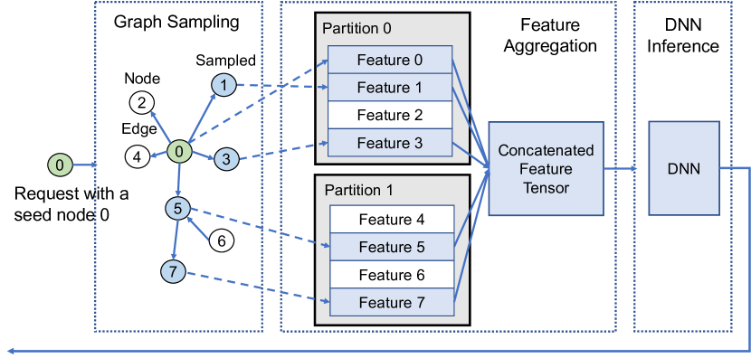
Figure 1. Overview of GNN serving computation

Fig. 1 gives shows the GNN serving computation, assuming a 2-layer sampling function. After receiving a GNN request with seed node 0, the system samples its neighbors and returns the layer-1 sampled nodes (1, 3, 5). When it reaches the layer-2 neighbors, it probabilistically samples node 7. After that, it collects the features for all sampled nodes (layer 0, node 0; layer 1, nodes 1, 3, 5; layer 2, node 7), potentially from different devices. It then concatenates the collected features, and the feature tensor is used for DNN inference. Finally, the inference results are returned to the user.

In practice, GNN serving must handle large graphs with many features: e.g., MAG240M (Hu et al., 2021), a heterogeneous academic graph dataset, has 240 million graph nodes, 1.7 billion edges, and 768-dimensional feature vectors for each node. Our production internet graph dataset has billions of graph nodes, with feature sizes totalling tens of TBs.

Therefore, features must be partitioned and distributed across servers. Each server comprises of multiple GPUs and dozens of CPU. Devices are inter-connected by a heterogeneous distributed NUMA fabric with NVLink, PCIe, Ethernet, and InfiniBand links (Li et al., 2023).

2.2. Challenges in large-scale GNN serving

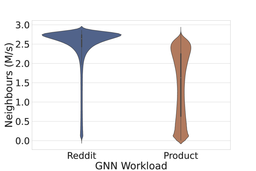
(a) Sampling [25,10] neighbors

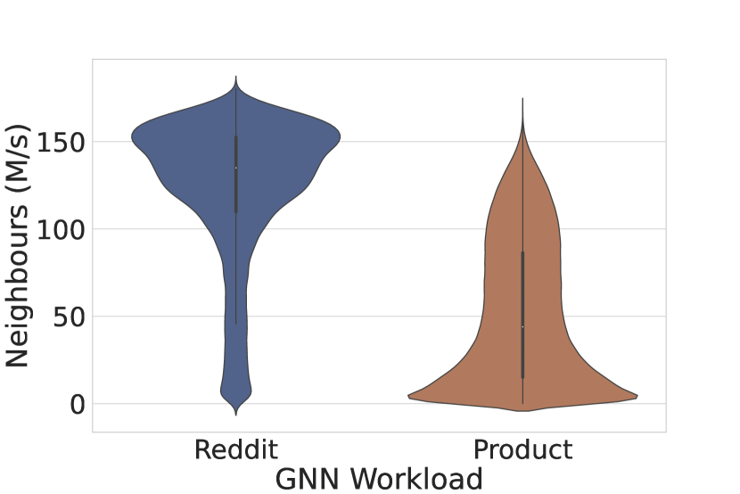
(b) Sampling [50,35] neighbors

Figure 2. Number of sampled neighbors (Reddit and Product)

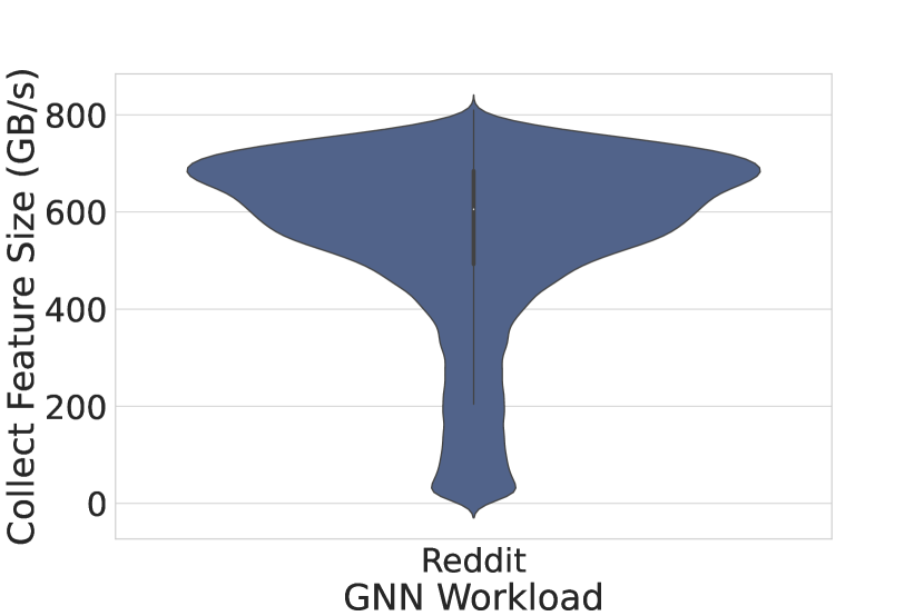
(a) Reddit graph

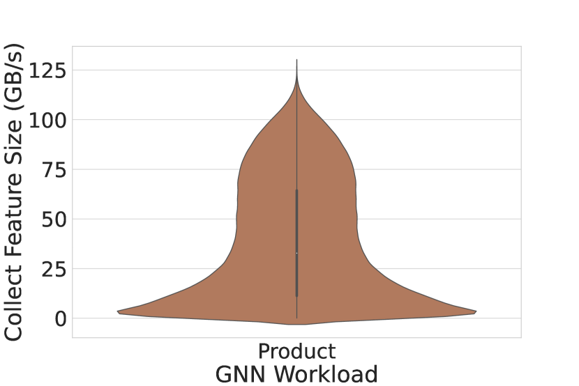
(b) Product graph

Figure 3. Size of aggregated features

Despite the processing scale, GNN requests must be served with low latency. For example, recommender systems must process thousands of requests within 15 ms (Zhou et al., 2018), stream processing handles millions of requests in milliseconds (Xu et al., 2021b; Mai et al., 2018), fraud detection systems must handle millions of requests within 20 ms (Xu et al., 2021a), and route planning applications process tens of millions of requests within 100 ms (He et al., 2021).

Due to the irregularity of the computation, it is challenging to achieve these latency goals. Real-world graph exhibit a high degree of skew in the number of neighbors associated with the graph nodes. When performing multi-layer neighbor sampling for a batch of GNN requests, systems may process substantially varying numbers of sampled neighbors and aggregated feature sizes.

We show this variability in sampled neighbors for two real-world graphs when handling a batch of 100,000 GNN requests. Each request requires sampling 25 layer-1 neighbors and 10 layer-2 neighbors. Fig. 2(a) shows that, for the Reddit graph (Hamilton et al., 2017a), the number of sampled neighbors ranges from 3,000 to 3,000,000, with the majority falling between 2,000,000 and 2,800,000. For the Product graph (Yang and Leskovec, 2012), the number of sampled neighbors ranges from 4,000 to 2,600,000.

This variability makes it challenging to map the sampling computation to a single type of device: CPU-based sampling provides predictably low latency, as CPUs can efficiently access graph data distributed across a large amount of memory, but their limited parallelism reduces throughput; in contrast, GPU-based sampling achieves higher throughput, but only when the GNN request samples many neighbors. A large number of neighbors fully utilizes the high degree of parallelism of GPUs and amortizes their higher start-up and data movement costs.

In addition to graph skew, the number of sampled neighbors is highly sensitive to the graph sampling configuration (i.e., the numbers of sampled layers and the number of neighbors per layer). Fig. 2(b) shows that, after adjusting the sampling configuration to include 50 layer-1 neighbors and 35 layer-2 neighbors, the distribution of sampled neighbors changes substantially: for the Reddit graph, the number of sampled neighbors now ranges from 10 million to 175 million; while for the Products graph, it varies between 2 million and 150 million, with the majority around 5 million.

We also examine the variability in the total size of aggregated features. Fig. 3(a) shows that the aggregated feature size for the Reddit graph ranges from 36 GB to 800 GB; for the Product graph (Fig. 3(b)), it ranges from 3 GB to 110 GB.

When using GPUs, all these features must be loaded into GPU memory for subsequent DNN computation. Transferring these features over the PCIe bus (with 16–32 GB/s bandwidth) incurs latencies from hundreds of milliseconds to tens of seconds. Such latencies are significantly higher than the GPU-based DNN computation time (usually in the tens of milliseconds), making feature aggregation a bottleneck.

2.3. GPU-based GNN serving

GNN serving systems require predictable low latency processing when exploiting GPUs. Existing GNN systems (e.g., PyG (Fey and Lenssen, 2019), DGL (Wang et al., 2019), GNNLab (Yang et al., 2022), BGL (Liu et al., 2021)) use GPUs for feature aggregation, and NextDoor (Jangda et al., 2021) uses GPUs for accelerating graph sampling. These systems however suffer limitations when using GPUs for serving:

Predictable latency on GPUs. Proposals to exploit GPUs for GNN sampling exist. NextDoor (Jangda et al., 2021) necessitates a large batch of seed nodes to fully utilize GPUs, but adversely affects latency performance in GNN serving.

DNN serving systems such as Clipper (Crankshaw et al., 2017) and Clockwork (Gujarati et al., 2020) use dynamic batching to reduce request latencies. They monitor the incoming DNN inference requests and construct dynamically-sized batches that can be processed by a given latency deadline. Such approaches, however, assume a constant computation and communication effort for a single request that targets a given DNN model: for a DNN inference request, the input data (e.g., image or text) is of a fixed size and leads to the same amount of activation data. This predictability makes it easier to aggregate requests until a given latency target is reached.

As we have shown in §2.2, GNN inference requests, however, require varying computational and communication resources. Since batches contain different graph seed nodes, there is a variance in the size of sampled graph nodes and thus aggregated features. This irregular computation makes simple batching techniques that assume a fixed cost per inference request infeasible.

Feature assignment to GPUs. Since feature data in GNN serving is large (see §2.2), the data must be distributed across GPU servers. Existing GNN systems, including DSP(Cai et al., 2023), BGL(Liu et al., 2021), GNNLab(Yang et al., 2022), cache popular features in GPUs, which requires a decision on feature popularity: GNNLab(Yang et al., 2022) estimates feature popularity by counting the feature’s access frequency during model training; BGL(Liu et al., 2021) ranks feature popularity based on their node in/out degrees in the graph.

However, such approaches are ineffective for GNN serving scenarios. When allocating features to servers, GNN serving systems cannot exploit prior information from training: the seed nodes during training are selected deliberately to follow a uniform distribution, which maximizes model accuracy. In contrast, seed nodes in GNN inference requests follow real-world skewed distributions (Kondor and Borgwardt, 2008). Training dataset also only includes a small subset of potential seed nodes (20%–30% in the OGB benchmark).

In addition, any method for feature assignment in GNN serving must take multi-layer neighbor sampling into account, otherwise the calculated feature popularity will deviate from those observed when serving GNNs.

3. Workload Aware GNN Serving

Next we introduce our idea of workload-aware GNN serving (§3.1) and give an overview of Quiver’s design (§3.2).

3.1. Overview

Our analysis in §2.2 reveals that the effectiveness of using GPUs for GNN serving depends on the properties of the graph. Therefore, we want to explore a design for a GNN serving system that is workload aware, i.e., the system makes decisions regarding the compute and data allocation to GPUs that depend on the graph properties.

Open challenges when realizing this idea is to decide (i) how and (ii) when to collect information about the workload. Our approach is to pre-compute workload metrics that capture properties of the graph used for GNN serving. If the system pre-computes appropriate metrics at deployment when the graph data is available, it can use the metrics for principled decision-making, both at deployment time when having to partition feature data from the graph across GPU servers and at runtime when assigning GNN inference computation to GPU and CPU devices. The cost of pre-computation of these metrics can be amortized across the execution of GNN requests.

We exploit two workload metrics in Quiver’s design:

Probabilistic sampled sub-graph size (PSGS). For a GNN request, the system must predict the computational load of the request to make a decision whether to execute the GNN sampling computation on a GPU or CPU: if the sampled neighborhood yields many nodes, GPU-based sampling is more efficient; if it results in few nodes, the sampling task can be executed by a CPU core with lower latency.

The PSGS metric estimates the number of sampled nodes for a given seed node in a graph, and the system can use it to allocate sampling tasks to the most appropriate device. It can be pre-calculated efficiently by GPUs(see §4.1). The pre-calculated values are stored in a lookup table, which fits into GPU memory (see §6.4) and is consulted by the system at runtime.

Feature access probability (FAP). The bulk of the data movement when serving GNN requests is due to the access of feature data. To prevent feature collection from becoming a communication bottleneck, the system must place features close (in terms of the NUMA/network topology) to the GPUs that access them. If a feature is popular, i.e., it has a high probability of access for any given GNN request, it should place within the NUMA/network topology in such a way that allows for lower latency access.

The FAP metric estimates the access likelihood of any feature data in the graph. It is calculated by GPUs by implementing graph sampling as sparse matrix multiplication (see §5.1). Based on the FAP value, the system can place feature data across multiple levels of the NUMA/network topology (from lowest to highest latency access): (1) local GPU; (2) GPU in the same server, interconnected via NVLink (He et al., 2022); (3) GPU in the same server, interconnect via PCIe; (4) GPU in the different server, interconnect with InfiniBand.

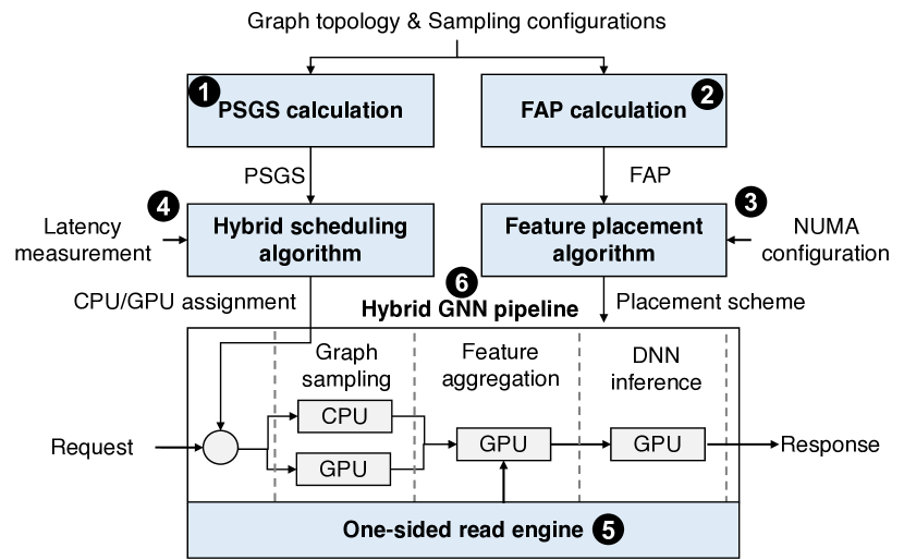
Figure 4. Quiver design

3.2. Design

Next describe the design of Quiver, a distributed GNN serving system for GPUs that uses the PSGS and FAP metrics for workload awareness. Figure 4 shows the design: Quiver takes a graph topology and sampling configurations as input at deployment time. These are used to pre-calculate the PSGS  and FAP metrics  , which is done efficiently by parallelizing the computation using GPUs (§4.1). For the PSGS metric, Quiver analyzes the relationship between the PSGS value and latency measurement of different emulation batches using a serving workload generator. It generates the relationship between PSGS and latency measurement, which allows Quiver to choose PSGS that can guide the assignment of GNN sampling to GPUs and CPUs.

After the FAP metric is calculated, a feature placement algorithm  uses it, in combination with information about the NUMA/network topology of the deployment, as input to decide on the feature assignment. It sorts the features based on the FAP metric and partitions and replicates features across the topology: it partitions popular features among GPUs, connected through NVLink and InfiniBand, thus caching popular features in GPUs and reducing PCIe traffic; for GPUs without NVLink and InfiniBand, Quiver replicates popular features to increase locality of access.

When processing GNN inference requests, a hybrid scheduling algorithm  dynamically assigns graph sampling tasks to GPUs and CPUs. It performs a PSGS lookup for each GNN request, and only assigns the request to GPUs when it improves throughput without increasing latency.

GNN requests are processed by a hybrid GNN pipeline  , which efficiently exploit a large number of GPU and CPU cores in executing different GNN computation stages (i.e., graph sampling, feature aggregation, and DNN inference), achieving high-throughput GNN request process.

As part of the pipeline, the features needed to execute feature aggregation tasks are collected by a one-sided read engine . If a feature can be accessed via NVLink and InfiniBand, the engine directly reads the feature from a peer GPUs/CPUs, avoiding interrupting CPUs and minimizing memory copies.

4. Workload-Aware GNN Sampling

In this section, we introduce the computation of PSGS (Section 4.1), describe how PSGS contributes to GNN sampling in achieving consistent latency performance (Section 4.2), and discuss how GNN serving pipeline can achieve high throughput (Section 4.3).

4.1. Estimation of probabilistic sampled subgraph size

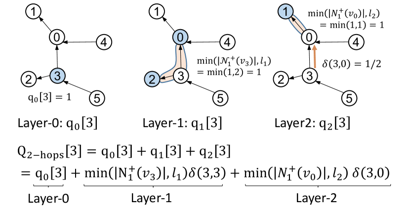
Figure 5. Probabilistic Sampled Sub-graph Size of Node 3

The estimation of the PSGS must account for the configuration of a probabilistic multi-layer neighbor sampling method. In the following, we use an example to describe how this configuration is involved in computing the PSGS and then give a formal definition.

Example. Fig 5 shows an example of the calculation of the PSGS of node 3 ($Q_{2-hops[3]}$). Assume the maximum sample size of hop-1 and hop-2 are 2 and 1 respectively. $Q_{2-hops}[3]$ is the sum of $\text{q}_{0}[3]$, $\text{q}_{1}[3]$ and $\text{q}_{2}[3]$, which represents the expected subgraph size at hop-0, hop-1 and hop-2 respectively.

$\text{q}_{0}[3]$ is always the subgraph with only the seed node, so the size is 1. The size of the hop-1 subgraph is 1, which is the minimum of the hop-1 neighbourhood size of 2 and the maximum sample size of 1, so $\text{q}_{1}[3]$ is 1. The probability that transits from node 3 to node 0 is $1/2$ and the subgraph size from 0 is 1, so $\text{q}_{2}[3]$ is $1\times 1/2=1/2$.

Construction algorithm. Specifically, the PSGS in $k$-hop sampling for a node $i$, denoted as ${Q}_{K-\text{hop}}[i]$, is defined as: $\text{Q}_{K-\text{hops}}[i]=\sum_{k=0}^{K}\text{q}_{k}[i]$ , where

$$\text{q}_{k}[i]=\begin{cases}1,&k=0\\ \sum_{v_{j}\in{N}^{+}_{k-1}(v_{i})}min(|{N}^{+}_{1}(v_{j})|,l_{k})\delta_{k-1}(i,j)\ ,&k>0\end{cases}$$

$\text{q}_{0}[i]$ refers to the probability sampled sub-graph size(PSGS) that each point can sample at the 0^th-layer, which is essentially the point itself. Therefore, $\text{q}_{0}[i]=1$. $\text{q}_{k}[i]$ represents the PSGS of node $i$ at the k^th-hop.

${N}^{+}_{k-1}(v_{i})$ defines the set of the k^th-hop out-neighbors of node $i$, which is the set of all nodes that can be sampled from node $i$ in the k^th-hop. $\delta_{k}(i,j)$ is the probability of sampling $v_{j}$ from $v_{i}$ at the k^th-hop (i.e., the transition probability). Both ${N}^{+}_{k-1}(v_{i})$ and $\delta_{k}(i,j)$ can be obtained by calculating the k^th-order weighted adjacency matrix $A^{k}=\prod^{k}A$. ${N}^{+}_{k-1}(v_{i})$ is the set of column indices corresponding to all non-zero elements in the $i$-th row of matrix $A^{k}$, and $\delta_{k}(i,j)=A^{k}[i][j]$

The output of this algorithm, $\text{Q}_{K-\text{hops}}$, is a lookup table stored in memory as an array, with a space complexity of $O(|V|)$. The time complexity for querying is $O(1)$.

Computation cost. When analyzing sampled sub-graph size, Quiver must compute the PSGS metric for each graph node. For the entire graph, the dominating computation cost lies in finding the set of K-hop out-degree neighbors of each node and the transition probabilities between each node in the graph at the K^th-hop. This requires calculating the K^th order weighted adjacency matrix $A^{K}$. The time complexity of this calculation using a CPU for serial matrix multiplication is $O(k|V|^{3})$.

Since most real-world graphs are sparse (e.g., the adjacency matrix is sparse) citeevidence, Quiver implements this process using a GPU. It employs CUDA’s sparse matrix multiplication operator, which reduces the time complexity to $O(k|V||E|)$, where $|E|<<|V|^{2}$ in sparse matrices. When analyzing a graph with hundreds of millions of graph nodes, the PSGS computation on a GPU can finish within minutes.

4.2. PSGS-guided hybrid sampling

Quiver can support GPUs to achieve predictable latency performance with the aid of PSGS. The main idea is to analyze the relationship between the PSGS and request processing latency offline. After being deployed, Quiver can monitor the seed nodes of GNN requests and estimate the PSGS of these requests. With the estimated PSGS, Quiver predicts the latency required for processing the requests. It assigns the request processing to GPUs only when it enhances throughput with predictable low latency.

4.2.1. PSGS and processing latency

We aim to predict the relationship between PSGS and request processing latency. To do this, we generate multiple GNN request batches with varying PSGS values. We then measure the processing latency of these batches in a hybrid sampling pipeline, shown by Figure 6(a). In this pipeline, graph sampling can be assigned to either CPUs or GPUs, while feature aggregation and DNN inference are assigned exclusively to GPUs.

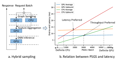
Figure 6. Relation between PSGS and GNN serving latency

Quiver is designed to ensure that offline latency measurements are accurate and consistent with those in a serving scenario. To achieve this, Quiver incorporates a serving workload generator that conducts latency measurements when both CPUs and GPUs are near full utilization, with no queuing in the pipeline. The serving workload generator continuously produces batches until there are a sufficient number of latency measurements for each PSGS, thus ensuring the reliability of the measurements.

After gathering an adequate number of latency measurements, Quiver generates a figure that illustrates the relationship between PSGS and the end-to-end processing latency of the hybrid sampling pipeline, as demonstrated in Figure 6(b). In this figure, we visualize both the average latency and the maximum latency achieved when using either GPUs or CPUs for GNN sampling. The maximum latency measurement enables Quiver to evaluate how to select a PSGS that complies with a latency bound, while the average latency measurement allows Quiver to choose a PSGS that targets a specific latency goal.

In the figure mentioned above, we observe the latency measurement lines intersect at 4 points: (a) CPU preferred. Point is where the CPU maximal latency intersects the GPU average latency. For any GNN request with a PSGS smaller than the CPU preferred point, this request can be completed faster on CPUs, even in the worst-case scenario. (b) GPU preferred. Point is where the CPU average latency intersects the GPU maximal latency. For any request with a PSGS larger than this point, sampling can be completed on GPUs with enhanced latency and throughput performance. (c) Latency preferred. Point is where the CPU maximal latency line intersects the GPU maximal latency line. If users prioritize bounding latency performance, they can select this cross point to guide the hybrid sampling: any GNN request with a PSGS smaller than the latency preferred point is assigned to CPUs. If larger, it is assigned to GPUs. (d) Throughput preferred. Point is where the CPU average latency line intersects the GPU average latency line. If users prioritize increasing throughput, they can choose this cross point to guide the hybrid sampling process.

4.2.2. GNN serving with PSGS

In the following, we explain how to utilize the selected PSGS value to enable efficient GNN serving while maintaining predictable performance. During GNN serving, the Quiver system continuously batches incoming GNN requests, completing the process once a batching deadline is reached. The Quiver system then iterates through all seed nodes within this batch, accumulating their PSGS estimations. If the accumulated sum is less than the user’s chosen PSGS value, the batch is assigned to CPUs for GNN sampling completion; otherwise, it is assigned to GPUs. This approach ensures that GPUs can deliver predictable low latency, while simultaneously directing the majority of the graph sampling workload to GPUs, thereby increasing throughput.

4.3. High-throughput hybrid pipelines

Designing high-throughput hybrid pipelines for GNN serving introduces several challenges. In the following, we discuss our design choices that address them:

(1) Multiplexing GNN pipelines in a processor. The processing of GNN requests require both compute-intensive stages (e.g., for graph sampling and DNN inference) and communication-intensive stages (e.g., for feature aggrgegation). A GNN pipeline can be thus interrupted for communication, leaving the processor idle. To address this, Quiver multiplexes multiple pipelines in one processor (e.g., with each pipeline running in a CUDA stream). Such a design allows the processor to process multiple requests concurrently, overlapping their computation and communication tasks (Koliousis et al., 2019).

(2) Sharing the queue for GNN pipelines in a processor. GNN requests with irregular computation patterns lead to diverse processing times on GPUs. To avoid dispatching batches to a slow pipeline, incurring significant queuing delays, Quiver creates a queue shared by the pipelines on the same processor. These pipelines compete for requests in the shared queue, avoiding queuing delays and stragglers.

(3) Sharing the graph for GPU pipelines in a server. GNN requests sample large graphs, which consumes substantial memory (e.g., 100s of GBs). GPUs, however, have limited memory (typically 16 GB–80 GB). To address this, Quiver replicates the graph topology in each server and makes all the GPU pipelines share this graph.

To make graph sharing efficient, we implement the shared graph using the GPU’s unified virtual addressing (UVA) memory. Each graph partition is implemented as a pinned memory block and directly mapped to the GPU’s memory space.

5. Workload-aware Feature Placement

In this section, we describe how Quiver computes the feature access probability (§5.1), places features on GPU servers (§5.2), and uses efficient one-sided GPU reads to access features (§5.3).

5.1. Estimation of feature access probabilities

Figure 7. Computing the feature access probability for node 3

The estimation of the feature access probability (FAP) is based on the following observation: a node’s feature is fetched from memory when the node is in the k-hop sampling subgraph of input seed nodes. Consequently, the more subgraphs a node feature is involved in, the higher the probability that the node feature is accessed. In the following, we use an example to explain the computation of this probability and then present a formal definition.

Example. Consider node 3 in the directed graph with equal edge weights shown in Fig. 7. We want to compute the probability of node 3 being sampled as a neighbor within 2 hops from other nodes, denoted as $\text{p}_{2-\text{hops}}[3]$. It is the sum of $p_{0}[3]$, $\text{p}_{1}[3]$, and $\text{p}_{2}[3]$, which represent the probabilities that node 3 is sampled within the 0^th, 1^st, and 2^nd layers, respectively.

Specifically, $\text{p}_{0}[3]=\frac{1}{6}$ is the probability that node 3 is selected from the 6 nodes as a seed node; $\text{p}_{1}[3]$ is the sum of the probabilities that node 3 is sampled from its one-hop neighbors (nodes 0 and 3). The probability that node 3 is sampled from node 0 is $\frac{1}{6}\times\frac{1}{2}$, and the probability from node 3 is $\frac{1}{6}\times 1$; and $\text{p}_{2}[3]$ is the probability that node 3 is sampled from its two-hop neighbor (node 4) via its one-hop neighbor (node 0). The probability that node 4 is sampled at the 0^th-layer is $\frac{1}{6}$, and the probabilities of transitioning from node 4 to node 0 and from node 0 to node 3 are $1$ and $\frac{1}{2}$, respectively. Thus, $\text{p}_{2}[3]$ is $\frac{1}{6}\times 1\times\frac{1}{2}=\frac{1}{12}$.

FAP definition and computation. Generally, the FAP of a node $v$ sampled within K-hops neighbor is computed recursively as follows: $\text{P}_{K-\text{hops}}[i]=\sum_{k=0}^{K}\text{p}_{k}[i]$ , where

$$\text{p}_{k}[i]=\begin{cases}c,&k=0\\ \sum_{v_{j}\in{N}^{-}_{k}(v_{i})}\text{p}_{0}(j)\ \delta_{k}(j,i),&k>0\end{cases}$$

$\text{p}_{0}[i]$ is the probability that node $i$ is sampled at the 0^th-layer and $\sum^{|V|}_{i=0}\text{q}_{0}[i]=1$, i.e., that node $i$ is directly requested as a seed node. If the probability of each node becoming a seed node is equal, then $\text{p}_{0}[i]=\frac{1}{|V|}$. Users can also set $\text{p}_{0}[i]$ based on the actual dataset; $\text{p}_{k}[i]$ denotes the probability that node $i$ can be sampled from other nodes in the k^th-hop.

${N}^{-}_{k}(v_{i})$ defines the set of k^th-layer in-neighbors of node $i$, which is the set of all nodes that can reach node $i$ in the k^th-hop. ${N}^{-}_{k}(v_{i})$ can be obtained by calculating the k^th-order weighted adjacency matrix $A^{k}=\prod^{k}A$. ${N}^{-}_{k}(v_{i})$ is the set of row indices corresponding to all non-zero elements in the $i$-th column of matrix $A^{k}$. This requires calculating the K^th order weighted adjacency matrix $A^{K}$. Using the previous analysis from §4, the time complexity of this calculation can be optemize by CUDA’s sparse matrix multiplication operator to $O(k|V||E|)$.

5.2. Feature placement

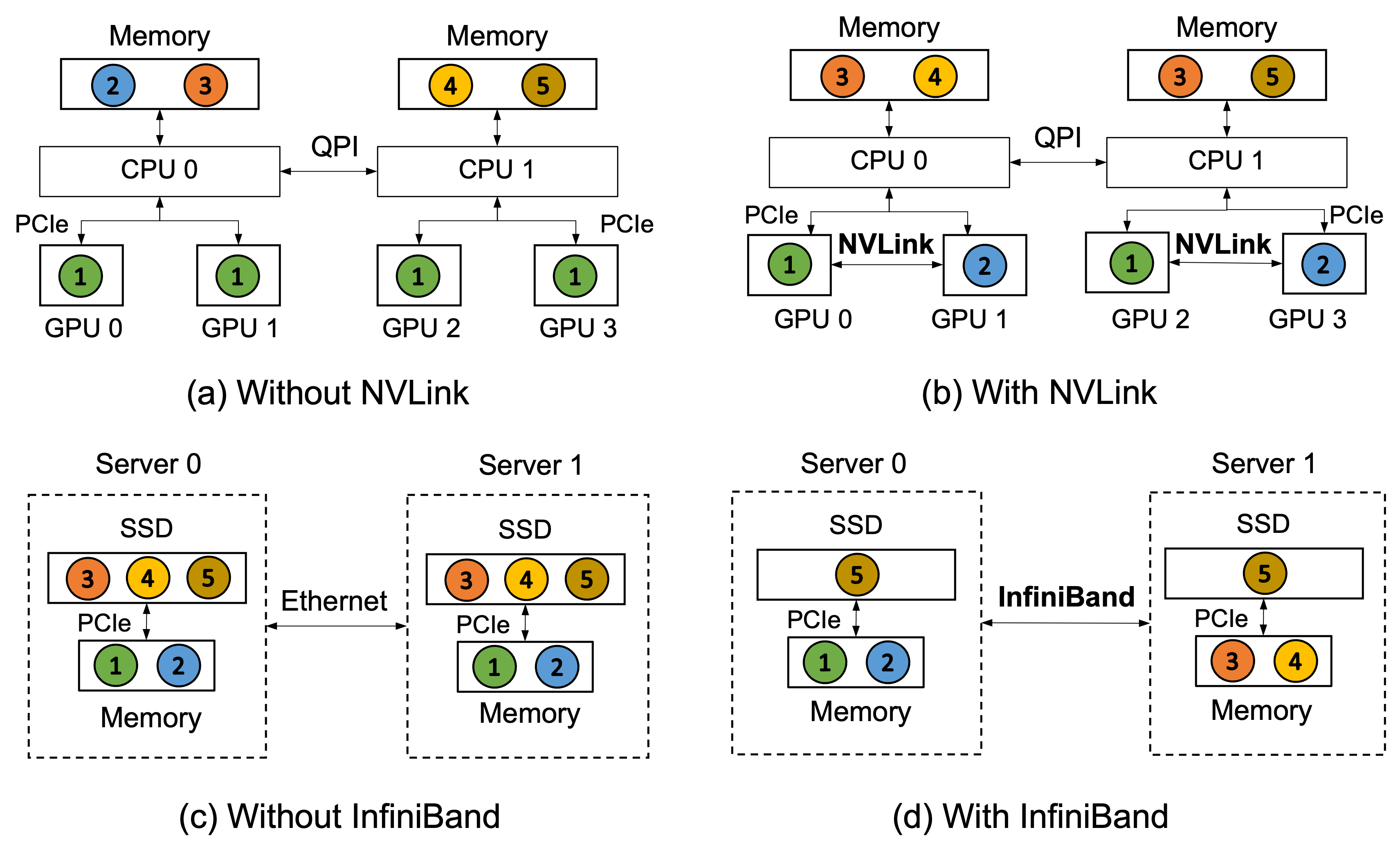
Figure 8. Feature placement scenarios

Quiver uses the FAP metric to place popular features strategically on GPUs. A primary objective of feature placement is to enable GPUs to take advantage of low-latency connectivity, such as NVLink and InfiniBand, to their peer GPUs. This allows GPUs to achieve low-latency access to features when aggregating features.

Minimizing the latency of feature aggregation presents a unique challenge: the features data is large and must be partitioned across servers. The feature aggregation latency is determined when all sampled features by a request become available in the GPU, allowing it to initiate DNN inference. In other words, this latency is equivalent to the tail latency of the last feature becoming available. This latency-driven minimization target makes the feature placement problem different from GNN training, which instead focuses on cache hit ratios (e.g., GNNLab (Yang et al., 2022), AliGraph (Zhu et al., 2019) and BGL (Liu et al., 2021)).

Impact of connectivity. Next, we derive insights from examples that show how NVLink and InfiniBand connectivity impact feature placement.

(a) Without NVLink. Fig. 8(a) shows feature placement in a server without NVLink. There are 5 features, and their FAP metrics decrease with their ID (i.e., feature 0 has the highest FAP value; feature 5 has the lowest). We assume that a server has two NUMA nodes, each with 1 CPU and 2 GPUs. The NUMA nodes are connected using a fast processor interconnect (e.g., UPI), and the CPU and GPU are connected using PCIe. The GPU’s high-bandwidth memory (HBM) can hold one feature, and the CPU memory can hold two features.

In this scenario, feature placement is not NVLink aware, and optimizes for data locality only. Consequently, it replicates feature 1 on all GPUs and evenly partitions the remaining features on the CPUs. Consider a GNN request that needs to aggregate features 1 and 2: the feature aggregation latency is determined by the latency of fetching feature 2 from the CPU to the GPU over the PCIe.

(b) With NVLink. Fig. 8(b) shows an improved feature placement that exploits NVLink. As NVLink offers high bandwidth and low data transfers to GPUs within the same NUMA node, fetching a feature over NVLink can be up to 50$\times$ faster than over PCIe. With this in mind, instead of replicating the most popular features on all GPUs, we can partition popular features and assign them to GPUs evenly. For example, feature 1 is placed in GPU 0 and feature 2 is placed in GPU 1. Since accessing data across NUMA nodes is costly, we can replicate features 1 and 2 in the GPUs in both NUMA nodes, still optimizing for data locality. This optimized feature placement strikes a balance between replication and partitioning, yielding improved feature aggregation latency. Consider again the request that must aggregate features 1 and 2: now GPU 0 fetches feature 2 from its peer GPU 1 over NVLink, while GPU 1 fetches feature 1 from GPU 0 over NVLink. This avoids fetching feature 2 over the slower PCIe bus, reducing aggregation latency.

(c) Without InfiniBand. Fig. 8(c) shows a scenario in which features must be placed across servers. Existing distributed feature placement methods (e.g., GNNLab, AliGraph, and BGL) assume that cross-server communication is slow (usually provided by Ethernet). They optimize for data locality, replicating popular features 1 and 2 on both servers and leaving the remaining features in the local disk.

Consider a GNN request that aggregates features 1, 2, and 3: feature 3 must be fetched from disk, incurring slow I/O operations, which increase feature aggregation latency.

(d) With InfiniBand. By making the placement InfiniBand aware, we can trade data locality for a fast InfiniBand link, thus partitioning popular features instead of replicating them. We assign features 1 and 2 to server 0 and the other popular features 3 and 4 to server 1.

When executing a GNN request that aggregates features 1, 2, and 3 on a GPU, the GPU can take advantage of the InfiniBand link by fetching feature 3 from the peer server. InfiniBand offers a bandwidth of up to 800 Gbps, which is 80$\times$ faster than conventional 10-Gbps Ethernet and SSDs. Consequently, feature aggregation latency is substantially improved compared to caching features locally.

Placement algorithm. We design an algorithm that takes into account NVLink/InfiniBand connectivity when placing features, minimizing feature aggregation latency. Its key steps are as follows: (i) Sort features: the placement algorithm begins by sorting all features based on their FAP values. The features have IDs in the range of $0$ to $N$; (ii) Analyze feature capacity per GPU: the algorithm considers number of features that can be placed in a GPU (denoted as the feature capacity). For this, Quiver requires the user to provide the number of GPUs $G$ in a server, the number of features that can be placed in a GPU $N_{g}$, and the number of NUMA nodes $C$ per server (We only consider the case in which GPUs are connected via NVLink in a NUMA node.) The resulting feature capacity is $\frac{G}{C}N_{g}$; (iii) Analyze feature capacity per server: the algorithm analyzes the feature capacity per server, denoted as $N_{s}$. If InfiniBand is used, $N_{s}=\frac{G}{C}N_{g}+N_{m}$, where $N_{m}$ represents the number of features that can be placed in server memory; otherwise, $N_{s}=\frac{G}{C}N_{g}+N_{m}+N_{d}$, where $N_{d}$ denotes the number of features that can be placed on disk; (iv) Partition and replicate (inter-server): based on $N_{s}$ and the number of servers $S$, the algorithm partitions the most popular features, with each partition containing $N_{s}$ features. It returns the most popular partition and replicates the features with IDs in the range of $[0:S\times N_{s}]$ in each server. Finally, it partitions the features with IDs in the range of $(S\times N_{s}:N]$: for each partitions, it sorts them according to their FAP values and initially places the features in the server memory. After exhausting memory, it places the remaining features on disk; and (v) Partition and replicate (intra-server): for each server, the algorithm replicates the features in the range of $[0:\frac{G}{C}N_{g}]$ across NUMA nodes. Within each NUMA node, it partitions the features, evenly assigning them to GPUs, so that each GPU has a similar aggregated FAP value.

5.3. Feature aggregation with one-sided reads

Quiver uses GPU kernels that can leverage efficient one-sided reads to access remote features over NVLink/InfiniBand. We describe how to support one-sided reads on GPUs and how to make them efficient.

Supporting one-sided reads on GPUs. Quiver supports one-sided reads on GPUs through a feature lookup table, which converts feature IDs to their physical memory addresses on a remote device. This feature lookup table is computed when executing the feature placement algorithm, and it can be accessed efficiently by the GPU kernels through UVA. Maintaining a feature lookup table incurs a low memory overhead: the number of rows in the table grows with the number of graph nodes. Even wit a large-scale graph that has hundreds of millions of graph nodes, the table only consumes several hundreds of MBs of memory.

Making one-sided reads efficient. Quiver uses GPU kernels with one-sided reads to access features that are sparsely distributed in memory spaces, i.e., their memory locations vary because the features are randomly sampled. To increase the efficiency of one-sided reads with sparse features, Quiver adopts two optimizations:

(i) Zero-copy optimization. Quiver implements one-sided reads by leveraging the zero-copy capabilities in CPU-GPU and GPU-GPU communication. To support zero-copy access to features on a peer GPU, Quiver registers the features as pinned memory using cudaHostRegister(), which allows CUDA kernels on local GPUs to access them directly. Before reading a batch of features from registered host memory, the features are sorted according to their addresses, which leads to better locality during feature address translation on GPUs.

To support zero-copy access over InfiniBand, Quiver registers the features as a memory region using ibv_reg_mr(). It then uses ibv_post_send() for one-sided RDMA reads, which avoids interrupting the CPU. Quiver allocates multiple queue pairs to parallelize RDMA reads, which improves throughput. Instead of setting the signal field and polling the completion queue for each read, Quiver performs it once for each batch, which further reduces latency.

(ii) TLB optimization. RDMA requires address translation in the InfiniBand NIC, but random memory accesses lead to TLB misses. Assuming the features have memory addresses ranging from $2k$ to $2k+1$ on the same memory page, when reading features e.g., at addresses $<$$2,3,10,11$$>$, the reading order of $<$$2,10,3,11$$>$ cause 4 TLB misses, whereas the order of $<$$2,3,10,11$$>$ results in only 2 TLB misses. Therefore, Quiver sorts all feature reads by their memory addresses, which allows adjacent reads to be clustered together to improve TLB hit rates of the NIC.

6. Evaluation

We evaluate the performance of Quiver experimentally. Quiver is written in C++, CUDA C, and Python. It can serve GNN models written in PyG and DGL (PyTorch). Our evaluation aims to answer the following questions:

• How does Quiver’s workload-aware approach compared to other GNN serving implementation in terms of latency and throughput? (§6.2)

• How does Quiver scale with more GPUs and servers? (§6.3)

• Does Quiver’s PSGS metric adapt to different request ingestion rates? (§6.4)

• Does Quiver’s FAP metric achieve better performance for feature access compared to existing algorithms? (§6.5)

• Does Quiver’s one-side read strategy achieve higher throughput when collection features? (§6.6)

• How is Quiver impacted by communication links? (§6.7)

6.1. Evaluation setup

Testbeds. We use the following hardware in our experiments: (i) Cluster testbed has 3 servers, each with 2 or 4 NVIDIA A6000 GPUs (with pairwise NVLink 3.0 links) and AMD EPYC 7402P 24-core CPUs with 128 GB of host memory. The network links connections are 100-Gbps InfiniBand; and (ii) Cloud testbed has 4 cloud VMs, each with 8 NVIDIA V100 GPUs (16 GB of RAM, with NVLink in a group of 4 GPUs) and Intel Xeon Gold 5220R (2.2 GHz) CPUs with 448 GB of host memory. The network is 10-Gbps Ethernet.

Dataset	Nodes	Edges	Feature size
ogbn-products	2.45M	123M	100
ogbn-papers100M	111M	1.6B	128
ogbn-mag240M	240M	1.72B	768
Reddit	232K	114M	300
LiveJournal	4.8M	69M	N/A
ogbn-products+	2.45M	123M	10000

Table 1. Evaluation datasets

Datasets. We use 6 public graph datasets (Tab. 1) : (i) ogbn-products (Hu et al., 2020b), a medium graph with product relations at Amazon; (ii) Reddit, a medium graph of social communities; (iii) ogbn-papers100M, a large graph of paper citation networks; (iv) ogbn-mag240M, a large graph of paper citation networks; (v) Live Journal, a medium graph of journal communities; and (vi) ogbn-products+, the Amazon product graph extended to have large features, matching our production workloads.

GNN models. We choose 2 popular GNN models: (i) GraphSAGE (Hamilton et al., 2017b), with k-hop neighbour sampling without replacement (hidden dimension of 256); and (ii) Graph Attention Network (GAT) (Veličković et al., 2017) with 4 attention heads. For both models, we use a local batch size of $1024$ on each worker. All models are implemented using PyG and PyTorch. We also evaluated other GNN models (GraphSaint (Zeng et al., 2019) and ClusterGCN (Chiang et al., 2019)), observing similar results (omitted due to space limitations).

Baselines. We compare Quiver against two state-of-the-art GNN systems, PyG (Fey and Lenssen, 2019) (v2.0.1) and DGL (Wang et al., 2019) (v0.7.0). We extend these systems to process GNN requests (i.e., using the test mode of PyG and DGL). Since Quiver supports models imported from PyG and DGL, we adopt their task implementations (e.g., for graph sampling, DNN inference) when possible. This way, performance differences can be attributed to the different request processing and feature placement.

Note that PaGraph (Lin et al., 2020), BGL (Liu et al., 2021) and GNNLab (Yang et al., 2022) support training only, and we could not extend them to supporting GNN serving. However, we re-implement the proposal by PaGraph for feature placement. Since P3 (Gandhi and Iyer, 2021) is not open-source, we also re-implement its approach in Quiver, reproducing its published performance results. While we exclude AliGraph (Zhu et al., 2019) from our end-to-end experiments, because it does not support PyTorch, we implement its feature placement approach.

Request workload. We launch multiple client processes that continuously produce GNN requests. Each request randomly samples input nodes with the out-degree as the weight, which is representative of real-world serving workloads.

6.2. Throughput and latency

To assess end-to-end performance, we measure the throughput and latency of serving a GNN model for a given dataset. We evaluate three scenarios: (i) users want the highest possible throughput with a given latency target; (ii) users want the lowest possible latency; and (iii) users want high throughput when serving large GNN models.

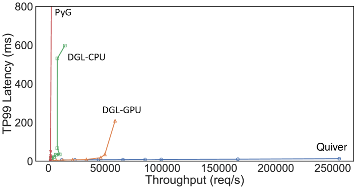
Figure 9. Throughput vs. latency of GNN request serving

Throughput vs. latency. First, we compare Quiver with PyG and DGL (with both CPU and GPU sampling) in terms of throughput and latency running on one server with 2 GPUs from the cluster testbed. We vary the batch size from 8 to 1024 to generate different scale workload and record the throughput and 99^th latency percentile. Fig. 9 shows the throughput/latency plot when processing GNN requests. We observe that the PyG’s latency increases substantially with a higher throughput to over 1 sec. DGL with CPU sampling behaves similarly, but DGL with GPU sampling achieves a higher throughput of just above 50,000 reqs/sec. In contrast, Quiver maintains latencies below 13 ms, despite processing requests at a peak throughput of 255,000 reqs/sec , when we have reached system full load, with CPU utilization at 95-100% and GPU utilization at 80-85%. Since Quiver only allocates sampling tasks that benefit from GPU processing to GPUs, while avoiding data movement bottlenecks between GPUs, it achieves a substantially higher throughput without a latency penalty.

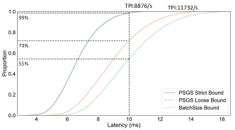
Figure 10. Latency with different policies

Strict vs. loose latency bounds. Quiver supports two settings for latency targets using the PSGS metric: PSGS-Strict, which apply upbound line to present the relationship between latency and PSGS, it strictly achieves a given latency bound; while PSGS-Loose, which use average line, it focuses on high throughput with a relaxed latency bound. We compare PSGS-Strict, PSGS-Loose, and a fixed batch size (Batchsize-Bound) as a baseline. We set the target 99^th percentile latency to 10 ms for PSGS and a fixed batch size that the most serves requests below 10 ms. Fig. 10 shows the CDF plot of the latency of PSGS-Strict, PSGS-Loose and Batchsize-Bound, which handle 99%, 73%, and 55% of queries within 10 ms, respectively. While having a higher latency bound, PSGS-Loose maintains higher throughput (11,700 reqs/sec), which is 57% higher than PSGS-Strict’s throughput (8,800 reqs/sec). This shows the flexibility of using the workload-aware PSGS metric, allowing it to be adjusted to different scenarios.

6.3. Scalability

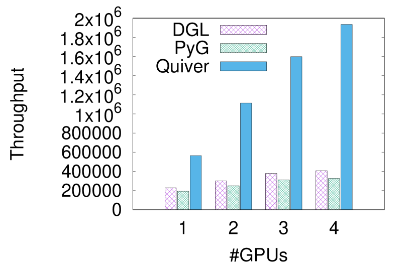
(a) ogbn-products

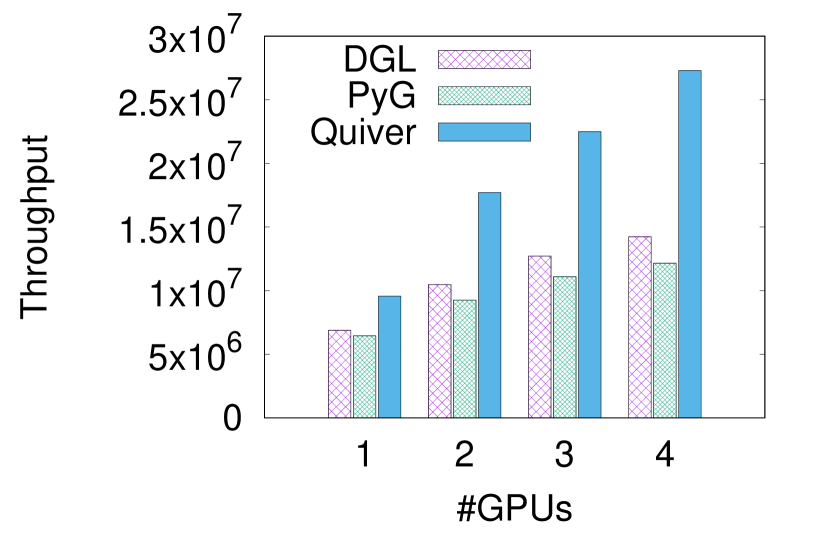
(b) ogbn-papers100M

Figure 11. Scalability with single multi-GPU server

Next we evaluate Quiver’s scalability. We increase the throughput until the systems reach a user latency threshold of 30 ms. We then report the achieved maximum throughput.

Single server. We first explore how well Quiver scales to multiple GPUs in a single server in our cluster testbed when serving the GraphSage model. Fig. 11 shows the achieve throughput with an increasing number of GPUs compared to PyG and DGL: with a small dataset (ogbn-products in Fig. 11(a)), Quiver handles 570,000 reqs/sec using a single GPU – in contrast, DGL and PyG achieves 220,000 reqs/sec (3.8$\times$ fewer) and 200,000 reqs/sec (4.7$\times$ fewer), respectively. Quiver benefits from exploiting multiple pipelines per GPU and its efficient one-sided reads; with 2–4 GPUs, Quiver is 8.3$\times$ and 10.1$\times$ faster than DGL and PyG, respectively. By caching features across GPUs based on the FAP metrics, Quiver achieves substantially higher throughput.

For the paper100M dataset (Fig. 11(b)), when running with 4 GPUs, Quiver benefits from larger total amount of GPU memory, which enables it to schedule more work to the GPUs. As a consequence, Quiver is 3.2$\times$ and 3.9$\times$ faster than DGL and PyG, respectively.

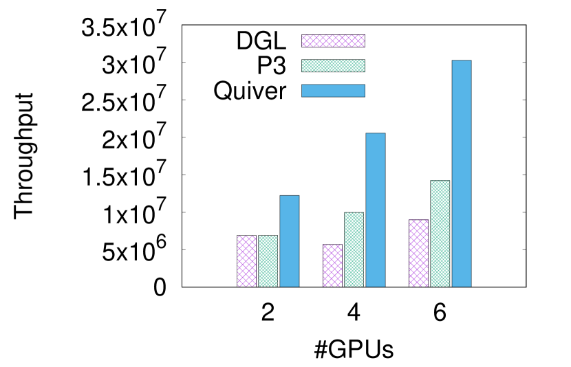
(a) Paper100M/GAT

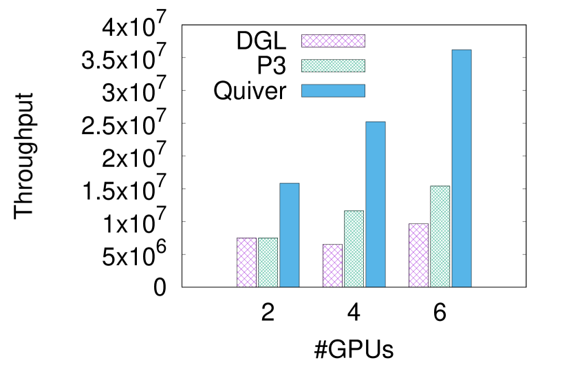
(b) Paper100M/GraphSage

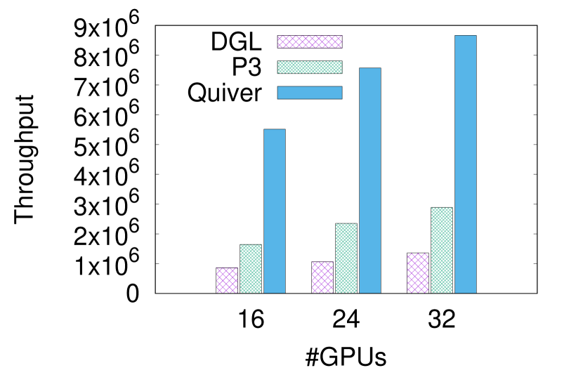
(c) Mag240M/GAT

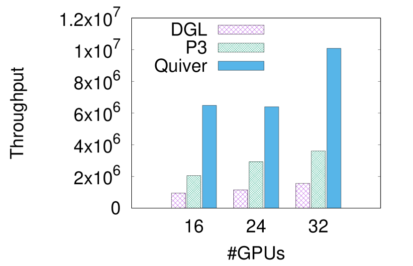
(d) Mag240M/GraphSage

Figure 12. Scalability with multiple multi-GPU servers

Cluster testbed. We use the cluster testbed with 3 servers (2 NVIDIA A6000 GPUs each). The 3 servers have sufficient memory to fit the paper100M dataset. DGL and P3 use their default strategies to partition the paper100M dataset. For GAT on a single server (2 GPUs) (see Fig. 12(a)), Quiver achieves a 2.8$\times$ speedup over both DGL and P3. With 2 servers (4 GPUs), P3 has better scalability compared to DGL, because it reduces the features sent over the network. P3 is thus 1.8$\times$ faster than DGL, which is consistent with the results from the P3 paper (Gandhi and Iyer, 2021). In contrast, Quiver achieves better scalability (3.2$\times$) than P3. Since Quiver replicates graph data and features in GPU memory, it can reduce communication costs. It also accounts for InfiniBand connectivity when deciding between partitioning and replication. Quiver’s throughput improves with more servers: with 3 servers (6 GPUs), it is 3.4$\times$ and 7.1$\times$ faster than P3 and DGL, respectively. For GraphSage (see Fig. 12(b)), Quiver achieves better results compared to GAT: with 3 servers (6 GPUs), it manages a 4.8$\times$ and 8.4$\times$ speedup compared to P3 and DGL, respectively. GraphSage places a strong emphasis on graph sampling and uses a smaller GNN model compared to GAT. This means that Quiver can more effectively optimize its feature placement, e.g., by placing more graph data and features in GPU memory due to the smaller GraphSage GNN size. It also increases the benefits of multiplexing GPU pipelines, e.g., by executing more feature aggregation, sampling tasks and DNN inference tasks on GPUs.

Cloud testbed. On the more powerful cloud testbed with up to 32 GPUs, we use the mag240M dataset, which is the largest GNN dataset in the OGB benchmark. With 2 servers (16 GPUs) (see Fig. 12(c)), Quiver achieves 5.5$\times$ and 2.8$\times$ the througput of DGL and P3, respectively, when serving the GAT model. With 4 servers (32 GPUs), Quiver improves the speedup ratios to 7$\times$ and 3.2$\times$, respectively. The same behavior can be also seen with GraphSage: with 32 GPU, Quiver achieves speedups of 7.9$\times$ and 3.3$\times$ compared to DGL and PyG, respectively. Note that these speed-up ratios are larger than those in the 16-GPU case.

Quiver’s performance improvement grows with the number of GPUs (or servers), because it fully utilizes the available CPU/GPU memory. With more servers, the CPU and GPU memory increases, but it leads to more intra-server communication. As a result, Quiver replicates more frequently-accessed feature data to improve locality, reducing the impact of these communication overheads. In contrast, DGL and P3 cannot fully exploit all cluster memory, and their scalability becomes limited by these network bottlenecks.

6.4. Robustness to data skew

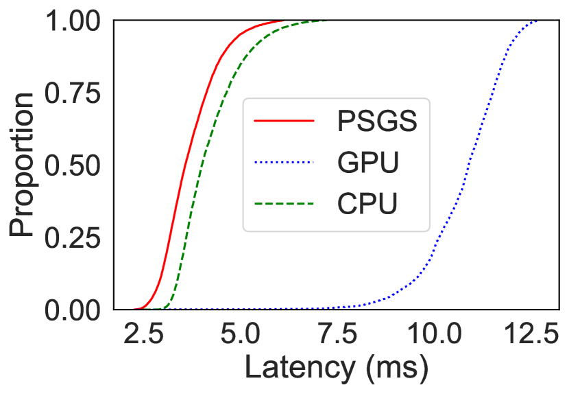
(a) Small workload

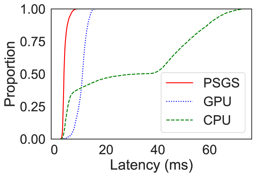
(b) Medium workload

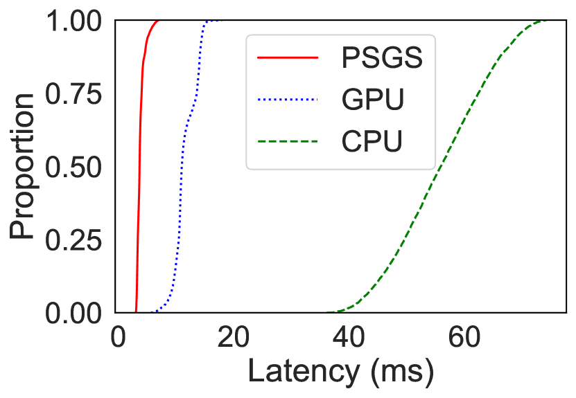
(c) Large workload

Figure 13. Different sampling strategies with skewed datasets

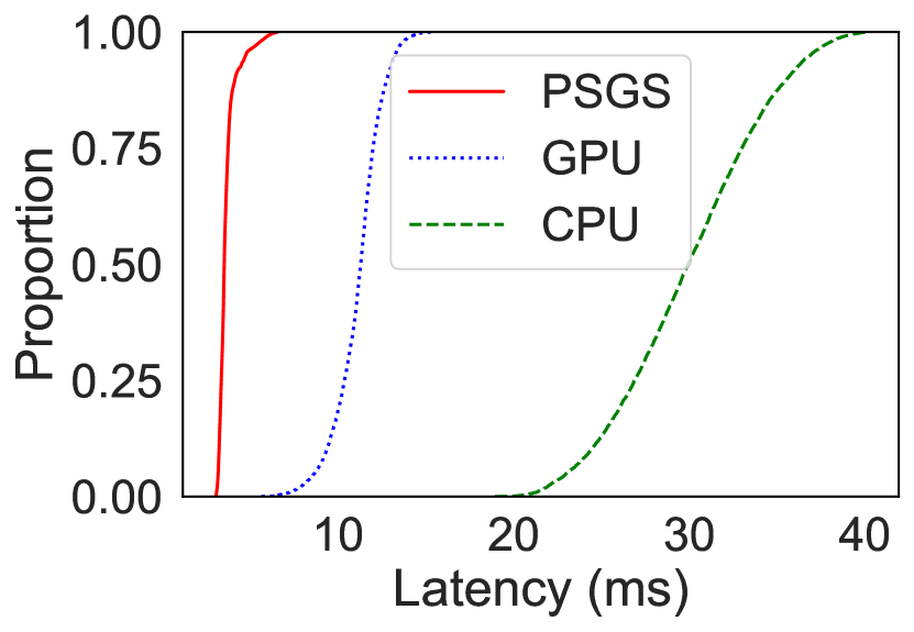
(a) Large batch size

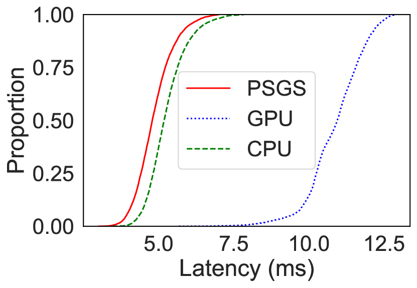
(b) Small batch size

Figure 14. Comparison of random sampling strategies

In this experiment, we investigate if Quiver’s PSGS metric yields the best performance when facing irregular input data. We use the reddit dataset and a 2-layer GraphSAGE model. The fan-out of each layer is set to 25 and 10, respectively. We use the cluster testbed with 2 NVIDIA A6000 GPUs. We compare three strategies: (i) our workload-aware PSGS strategy for sampling; (ii) CPU-based sampling; and (iii) GPU-based sampling. For each strategy, we use a batch size of 96 to construct the initial nodes and then perform neighbor sampling on the dataset to obtain different workloads: for example, we select nodes with high degrees and low degrees as seeds in the large and small workloads, respectively. The small workload contains 4$\times$; the medium workload contains 170$\times$; and the large workload contains 280$\times$ the initial nodes. Fig. 13 shows that the PSGS strategy achieves the best performance in all cases: with the large workload, the GPU-based strategy performs better than the CPU-based strategy. It utilizes the GPU’s ability for high throughput/low latency computation for sampling; with the small workload, the CPU-based strategy performs better, because it can reduces the overhead of data transfers between CPUs and GPUs. We also compare the performance of the strategies with different batch sizes. We use a small batch size of 4 and a large batch size of 96. We randomly sample batches and perform two-layer neighbour sampling. As Fig. 13 shows, we observe the same trend as in Fig. 13: PSGS achieves the best performance irrespective of the batch size: with large batches, the GPU-based strategy performs better than the CPU-based strategy; with small batches, the CPU-based strategy performs better than the GPU-based strategy.

6.5. Effectiveness of feature placement

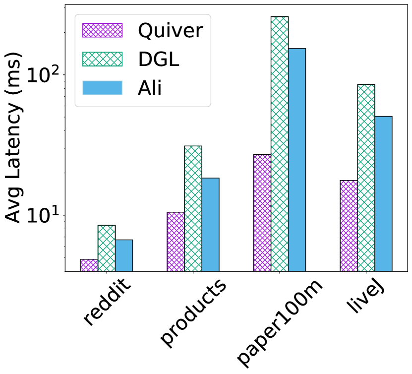
(a) 2 servers

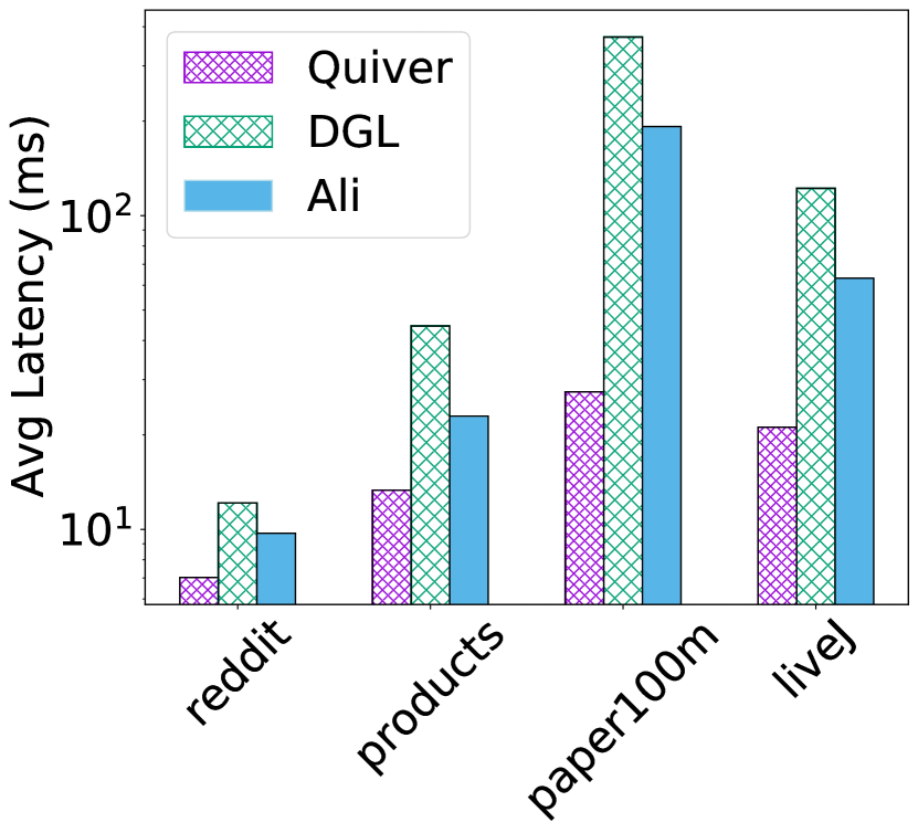
(b) 8 servers

Figure 15. Latency impact of feature placement

We evaluate Quiver’s workload-aware feature placement using the FAP metric on 2 and 8 servers. We compare against two baselines using 4 datasets (Reddit, ogbn-products, ogbn-papers100m, LiveJ): (i) hash-based graph partitioning, which is the default for DGL; and (ii) importance-based graph partitioning, which is used by AliGraph (Zhu et al., 2019). The latter considers the degrees of graph nodes and performs a balanced graph cut, which is similar to Metis (Karypis and Kumar, 1997). We allow all devices to have 20% extra memory to replicate data. DGL uses halo nodes to cache hot data; AliGraph uses an LRU cache for recently accessed data. Fig. 15 shows that Quiver outperforms DGL and AliGraph in terms of serving latency across all datasets and platforms: on the Reddit dataset, Quiver has a serving latency of 4.9 ms and 7.0 ms on 2 and 8 servers, respectively; DGL and AliGraph achieve latencies of 8.5 ms and 6.7 ms on 2 machines, and 12.2 ms and 9.7 ms on 8 machines, respectively. As the number of servers increases from 2 to 8, the serving latency increases for all platforms and datasets. This can be attributed to the increased communication overhead in a distributed setting: with 8 devices, as shown in Fig. 15(b), the performance of hash-based partitioning (DGL) quickly degrades (e.g., for paper100m, the latency grows from 259 ms to 370 ms) because it is workload-agnostic. The performance of AliGraph also slightly decreases (e.g., for paper100m, the latency grows from 153 ms to 192 ms compared to the 2-device case). In contrast, Quiver sustains a low latency that is much lower than AliGraph across all datasets. We speculate that Quiver’s performance improvement over DGL and AliGraph will become even more significant for larger deployments due to its more accurate estimation of data access probabilities and its use of replication.

6.6. Performance of feature collection

(a) Paper100M

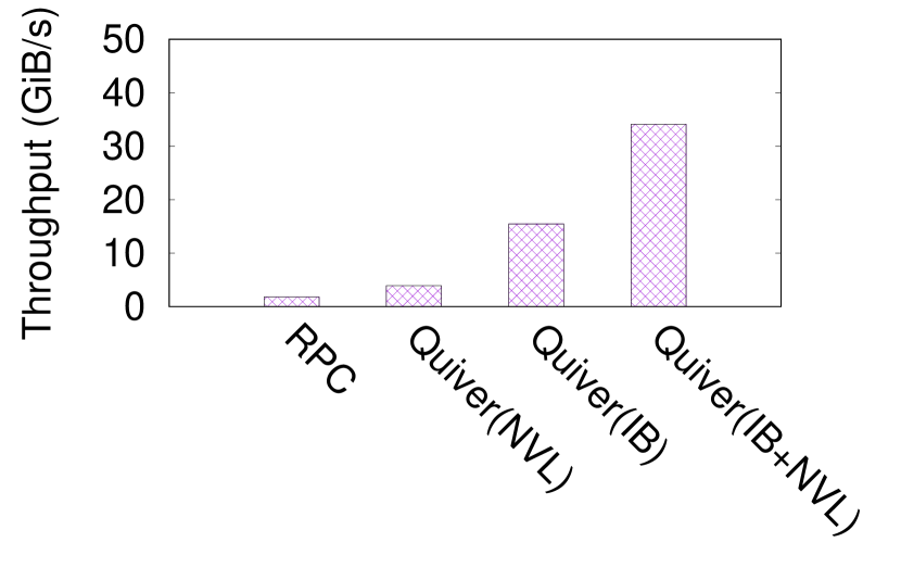
(b) Mag240M

Figure 16. Throughput of feature collection

Finally, we evaluate the performance of feature collection in Quiver. We measure the throughput of collecting the feature data of graph nodes (usually more than 150,000) in a batch of size 1024 under GraphSage with 2-layer sampling. We compare Quiver with a state-of-the-art RPC library, TensorPipe (ten, [n. d.]), which is the high-performance NCCL-backed RPC library of PyTorch, as used by DGL. We deploy the experiment on the cluster testbed with 3 servers interconnected by InfiniBand. Each pair of GPUs uses NVLink. For the paper100M dataset (see Fig. 16(a)), the RPC library collects features at the rate of 3 GB/s, but Quiver’s feature collection achieves 7 GB/s using NVLink. With InfiniBand, avoiding the slower Ethernet links, Quiver reaches 18 GB/s. Since Quiver can leverage both NVLink and InfiniBand, it achieves a combined throughput up to 40 GB/s, which is 13$\times$ higher than that of the RPC library. We observe a similar performance improvement for the larger dataset, such as mag240M (see Fig. 16(b)). Quiver’s high feature collection throughput shows the benefit of using GPUs for feature aggregation together with one-sided reads that employ CPU by-pass, surpassing the performance of conventional approaches that coordinate GPU’s collective communication through CPUs (Mai et al., 2020).

6.7. Impact of communication links

We report Quiver’s performance (in terms of latency) in different network configurations: Quiver without InfiniBand and Quiver without NVLink. Specifically, we disable InfiniBand by using SSD as the storage backend, and we disable NVLink by following the strategy shown in Fig. 8. When we disable InfiniBand for the mag240m dataset, the latency grows by 1.6$\times$ from 30.2 ms to 48.9 ms. When we disable NVLink for the paper100m dataset, the latency grows by 1.5$\times$ from 27.4 ms to 41.2 ms. Without the faster connectivity, the communication between servers and the GPUs must involve the CPU, which is slower.

7. Conclusions

We described Quiver, a new low-latency GPU-based GNN serving system that is workload-aware. Quiver achieves low-latency by dynamically batching requests based on latency predictions that account for the sampled sub-graph size. Our experimental results show that Quiver substantially surpasses the performance of existing distributed GNN serving systems.

8. Acknowledgement

We thank the constructive feedback from Wenting Shen, Ye Li, Xiaoming Qin, Lingguan Yang and Kun Zhao for improving the development of an early version of Quiver.

References

- (1)
- gra ([n. d.]) [n. d.]. GraphLearn-for-PyTorch(GLT). https://github.com/alibaba/graphlearn-for-pytorch.
- ten ([n. d.]) [n. d.]. TensorPipe. https://github.com/pytorch/tensorpipe/.
- Addanki et al. (2021) Ravichandra Addanki, Peter W Battaglia, David Budden, Andreea Deac, Jonathan Godwin, Thomas Keck, Wai Lok Sibon Li, Alvaro Sanchez-Gonzalez, Jacklynn Stott, Shantanu Thakoor, et al. 2021. Large-scale graph representation learning with very deep gnns and self-supervision. arXiv preprint arXiv:2107.09422 (2021).
- Cai et al. (2023) Zhenkun Cai, Qihui Zhou, Xiao Yan, Da Zheng, Xiang Song, Chenguang Zheng, James Cheng, and George Karypis. 2023. DSP: Efficient GNN training with multiple GPUs. In Proceedings of the 28th ACM SIGPLAN Annual Symposium on Principles and Practice of Parallel Programming. 392–404.
- Chiang et al. (2019) Wei-Lin Chiang, Xuanqing Liu, Si Si, Yang Li, Samy Bengio, and Cho-Jui Hsieh. 2019. Cluster-gcn: An efficient algorithm for training deep and large graph convolutional networks. In Proceedings of the 25th ACM SIGKDD International Conference on Knowledge Discovery and Data Mining. 257–266.
- Crankshaw et al. (2017) Daniel Crankshaw, Xin Wang, Guilio Zhou, Michael J Franklin, Joseph E Gonzalez, and Ion Stoica. 2017. Clipper: A Low-Latency Online Prediction Serving System. In 14th USENIX Symposium on Networked Systems Design and Implementation (NSDI 17). 613–627.
- Fan et al. (2019) Wenqi Fan, Yao Ma, Qing Li, Yuan He, Eric Zhao, Jiliang Tang, and Dawei Yin. 2019. Graph neural networks for social recommendation. In The world wide web conference. 417–426.
- Fey and Lenssen (2019) Matthias Fey and Jan E. Lenssen. 2019. Fast Graph Representation Learning with PyTorch Geometric. In ICLR Workshop on Representation Learning on Graphs and Manifolds.
- Gandhi and Iyer (2021) Swapnil Gandhi and Anand Padmanabha Iyer. 2021. P3: Distributed Deep Graph Learning at Scale. In 15th USENIX Symposium on Operating Systems Design and Implementation (OSDI 21). 551–568.
- Gao et al. (2018) Pin Gao, Lingfan Yu, Yongwei Wu, and Jinyang Li. 2018. Low latency RNN inference with cellular batching. In Proceedings of the Thirteenth EuroSys Conference. 1–15.
- Gujarati et al. (2020) Arpan Gujarati, Reza Karimi, Safya Alzayat, Wei Hao, Antoine Kaufmann, Ymir Vigfusson, and Jonathan Mace. 2020. Serving DNNs like Clockwork: Performance Predictability from the Bottom Up. In 14th USENIX Symposium on Operating Systems Design and Implementation (OSDI 20). 443–462.
- Guo et al. (2019) Shengnan Guo, Youfang Lin, Ning Feng, Chao Song, and Huaiyu Wan. 2019. Attention Based Spatial-Temporal Graph Convolutional Networks for Traffic Flow Forecasting. In Proceedings of the Thirty-Third AAAI Conference on Artificial Intelligence and Thirty-First Innovative Applications of Artificial Intelligence Conference and Ninth AAAI Symposium on Educational Advances in Artificial Intelligence (Honolulu, Hawaii, USA) (AAAI’19/IAAI’19/EAAI’19). AAAI Press, Article 114, 8 pages. https://doi.org/10.1609/aaai.v33i01.3301922
- Hamilton et al. (2017a) Will Hamilton, Zhitao Ying, and Jure Leskovec. 2017a. Inductive representation learning on large graphs. Advances in neural information processing systems 30 (2017).
- Hamilton et al. (2017b) William L. Hamilton, Rex Ying, and Jure Leskovec. 2017b. Inductive Representation Learning on Large Graphs. In Proceedings of the 31st International Conference on Neural Information Processing Systems (Long Beach, California, USA) (NIPS’17). Curran Associates Inc., Red Hook, NY, USA, 1025–1035.
- He et al. (2021) Congjie He, Haowei Wang, Xinrui Jiang, Meng Ma, and Ping Wang. 2021. Dyna-PTM: OD-enhanced GCN for Metro Passenger Flow Prediction. In 2021 International Joint Conference on Neural Networks (IJCNN). 1–9. https://doi.org/10.1109/IJCNN52387.2021.9534153
- He et al. (2022) Yuqi He, Zhiquan Lai, Zhejiang Ran, Lizhi Zhang, and Dongsheng Li. 2022. SCGraph: Accelerating Sample-based GNN Training by Staged Caching of Features on GPUs. In 2022 IEEE Intl Conf on Parallel & Distributed Processing with Applications, Big Data & Cloud Computing, Sustainable Computing & Communications, Social Computing & Networking (ISPA/BDCloud/SocialCom/SustainCom). IEEE, 106–113.
- Hu et al. (2021) Weihua Hu, Matthias Fey, Hongyu Ren, Maho Nakata, Yuxiao Dong, and Jure Leskovec. 2021. Ogb-lsc: A large-scale challenge for machine learning on graphs. arXiv preprint arXiv:2103.09430 (2021).
- Hu et al. (2020a) Weihua Hu, Matthias Fey, Marinka Zitnik, Yuxiao Dong, Hongyu Ren, Bowen Liu, Michele Catasta, and Jure Leskovec. 2020a. Open graph benchmark: Datasets for machine learning on graphs. Advances in neural information processing systems 33 (2020), 22118–22133.
- Hu et al. (2020b) Weihua Hu, Matthias Fey, Marinka Zitnik, Yuxiao Dong, Hongyu Ren, Bowen Liu, Michele Catasta, and Jure Leskovec. 2020b. Open Graph Benchmark: Datasets for Machine Learning on Graphs. arXiv preprint arXiv:2005.00687 (2020).
- Jangda et al. (2021) Abhinav Jangda, Sandeep Polisetty, Arjun Guha, and Marco Serafini. 2021. Accelerating Graph Sampling for Graph Machine Learning Using GPUs. In Proceedings of the Sixteenth European Conference on Computer Systems (Online Event, United Kingdom) (EuroSys ’21). Association for Computing Machinery, New York, NY, USA, 311–326. https://doi.org/10.1145/3447786.3456244
- Karypis and Kumar (1997) George Karypis and Vipin Kumar. 1997. METIS: A software package for partitioning unstructured graphs, partitioning meshes, and computing fill-reducing orderings of sparse matrices. (1997).
- Koliousis et al. (2019) Alexandros Koliousis, Pijika Watcharapichat, Matthias Weidlich, Luo Mai, Paolo Costa, and Peter Pietzuch. 2019. Crossbow: Scaling deep learning with small batch sizes on multi-gpu servers. arXiv preprint arXiv:1901.02244 (2019).
- Kondor and Borgwardt (2008) Risi Kondor and Karsten M Borgwardt. 2008. The skew spectrum of graphs. In Proceedings of the 25th international conference on Machine learning. 496–503.
- Krishnamurthy et al. (2023) Gangeshwar Krishnamurthy, Navonil Majumder, Soujanya Poria, and Erik Cambria. 2023. A deep learning approach for multimodal deception detection. In Computational Linguistics and Intelligent Text Processing: 19th International Conference, CICLing 2018, Hanoi, Vietnam, March 18–24, 2018, Revised Selected Papers, Part I. Springer, 87–96.
- Li et al. (2023) Huaicheng Li, Daniel S Berger, Lisa Hsu, Daniel Ernst, Pantea Zardoshti, Stanko Novakovic, Monish Shah, Samir Rajadnya, Scott Lee, Ishwar Agarwal, et al. 2023. Pond: CXL-based memory pooling systems for cloud platforms. In Proceedings of the 28th ACM International Conference on Architectural Support for Programming Languages and Operating Systems, Volume 2. 574–587.
- Lin et al. (2020) Zhiqi Lin, Cheng Li, Youshan Miao, Yunxin Liu, and Yinlong Xu. 2020. Pagraph: Scaling gnn training on large graphs via computation-aware caching. In Proceedings of the 11th ACM Symposium on Cloud Computing. 401–415.
- Liu et al. (2021) Tianfeng Liu, Yangrui Chen, Dan Li, Chuan Wu, Yibo Zhu, Jun He, Yanghua Peng, Hongzheng Chen, Hongzhi Chen, and Chuanxiong Guo. 2021. Bgl: Gpu-efficient gnn training by optimizing graph data i/o and preprocessing. arXiv preprint arXiv:2112.08541 (2021).
- Lu et al. (2022) Mingxuan Lu, Zhichao Han, Susie Xi Rao, Zitao Zhang, Yang Zhao, Yinan Shan, Ramesh Raghunathan, Ce Zhang, and Jiawei Jiang. 2022. BRIGHT - Graph Neural Networks in Real-Time Fraud Detection. In Proceedings of the 31st ACM International Conference on Information and Knowledge Management (Atlanta, GA, USA) (CIKM ’22). Association for Computing Machinery, New York, NY, USA, 3342–3351. https://doi.org/10.1145/3511808.3557136
- Mai et al. (2020) Luo Mai, Guo Li, Marcel Wagenländer, Konstantinos Fertakis, Andrei-Octavian Brabete, and Peter Pietzuch. 2020. KungFu: Making Training in Distributed Machine Learning Adaptive. In 14th USENIX Symposium on Operating Systems Design and Implementation (OSDI 20). USENIX Association, 937–954. https://www.usenix.org/conference/osdi20/presentation/mai
- Mai et al. (2018) Luo Mai, Kai Zeng, Rahul Potharaju, Le Xu, Steve Suh, Shivaram Venkataraman, Paolo Costa, Terry Kim, Saravanan Muthukrishnan, Vamsi Kuppa, et al. 2018. Chi: A scalable and programmable control plane for distributed stream processing systems. Proceedings of the VLDB Endowment 11, 10 (2018), 1303–1316.
- Min et al. (2021) Seung Won Min, Kun Wu, Sitao Huang, Mert Hidayetoğlu, Jinjun Xiong, Eiman Ebrahimi, Deming Chen, and Wen-mei Hwu. 2021. Pytorch-direct: Enabling gpu centric data access for very large graph neural network training with irregular accesses. arXiv preprint arXiv:2101.07956 (2021).
- Sanchez-Gonzalez et al. (2020) Alvaro Sanchez-Gonzalez, Jonathan Godwin, Tobias Pfaff, Rex Ying, Jure Leskovec, and Peter Battaglia. 2020. Learning to simulate complex physics with graph networks. In International conference on machine learning. PMLR, 8459–8468.
- Sima et al. (2022) Chijun Sima, Yao Fu, Man-Kit Sit, Liyi Guo, Xuri Gong, Feng Lin, Junyu Wu, Yongsheng Li, Haidong Rong, Pierre-Louis Aublin, and Luo Mai. 2022. Ekko: A Large-Scale Deep Learning Recommender System with Low-Latency Model Update. In 16th USENIX Symposium on Operating Systems Design and Implementation (OSDI 22). USENIX Association, Carlsbad, CA, 821–839. https://www.usenix.org/conference/osdi22/presentation/sima
- Veličković et al. (2017) Petar Veličković, Guillem Cucurull, Arantxa Casanova, Adriana Romero, Pietro Lio, and Yoshua Bengio. 2017. Graph attention networks. arXiv preprint arXiv:1710.10903 (2017).
- Wang et al. (2019) Minjie Wang, Da Zheng, Zihao Ye, Quan Gan, Mufei Li, Xiang Song, Jinjing Zhou, Chao Ma, Lingfan Yu, Yu Gai, Tianjun Xiao, Tong He, George Karypis, Jinyang Li, and Zheng Zhang. 2019. Deep Graph Library: A Graph-Centric, Highly-Performant Package for Graph Neural Networks. arXiv preprint arXiv:1909.01315 (2019).
- Wang et al. (2018) Yue Wang, Yongbin Sun, Ziwei Liu, Sanjay E. Sarma, Michael M. Bronstein, and Justin M. Solomon. 2018. Dynamic Graph CNN for Learning on Point Clouds. https://doi.org/10.48550/ARXIV.1801.07829
- Wu et al. (2020) Shiwen Wu, Wentao Zhang, Fei Sun, and Bin Cui. 2020. Graph Neural Networks in Recommender Systems: A Survey. CoRR abs/2011.02260 (2020). arXiv:2011.02260 https://arxiv.org/abs/2011.02260
- Xie et al. (2021) Lingqiang Xie, Dechang Pi, Xiangyan Zhang, Junfu Chen, Yi Luo, and Wen Yu. 2021. Graph neural network approach for anomaly detection. Measurement 180 (2021), 109546.
- Xu et al. (2021a) Bingbing Xu, Huawei Shen, Bingjie Sun, Rong An, Qi Cao, and Xueqi Cheng. 2021a. Towards consumer loan fraud detection: Graph neural networks with role-constrained conditional random field. In Proceedings of the AAAI Conference on Artificial Intelligence, Vol. 35. 4537–4545.
- Xu et al. (2021b) Le Xu, Shivaram Venkataraman, Indranil Gupta, Luo Mai, and Rahul Potharaju. 2021b. Move Fast and Meet Deadlines: Fine-grained Real-time Stream Processing with Cameo. In 18th USENIX Symposium on Networked Systems Design and Implementation (NSDI 21). USENIX Association, 389–405. https://www.usenix.org/conference/nsdi21/presentation/xu
- Yang and Leskovec (2012) Jaewon Yang and Jure Leskovec. 2012. Defining and evaluating network communities based on ground-truth. In Proceedings of the ACM SIGKDD Workshop on Mining Data Semantics. 1–8.
- Yang et al. (2022) Jianbang Yang, Dahai Tang, Xiaoniu Song, Lei Wang, Qiang Yin, Rong Chen, Wenyuan Yu, and Jingren Zhou. 2022. GNNLab: a factored system for sample-based GNN training over GPUs. In Proceedings of the Seventeenth European Conference on Computer Systems. 417–434.
- Ying et al. (2018) Rex Ying, Ruining He, Kaifeng Chen, Pong Eksombatchai, William L Hamilton, and Jure Leskovec. 2018. Graph convolutional neural networks for web-scale recommender systems. In Proceedings of the 24th ACM SIGKDD International Conference on Knowledge Discovery and Data Mining. 974–983.
- Zeng et al. (2019) Hanqing Zeng, Hongkuan Zhou, Ajitesh Srivastava, Rajgopal Kannan, and Viktor Prasanna. 2019. Graphsaint: Graph sampling based inductive learning method. arXiv preprint arXiv:1907.04931 (2019).
- Zhang and Zitnik (2020) Xiang Zhang and Marinka Zitnik. 2020. GNNGuard: Defending Graph Neural Networks against Adversarial Attacks. In Advances in Neural Information Processing Systems, H. Larochelle, M. Ranzato, R. Hadsell, M.F. Balcan, and H. Lin (Eds.), Vol. 33. Curran Associates, Inc., 9263–9275. https://proceedings.neurips.cc/paper/2020/file/690d83983a63aa1818423fd6edd3bfdb-Paper.pdf
- Zhang et al. (2018) Ziwei Zhang, Peng Cui, and Wenwu Zhu. 2018. Deep Learning on Graphs: A Survey. CoRR abs/1812.04202 (2018). arXiv:1812.04202 http://arxiv.org/abs/1812.04202
- Zheng et al. (2021) Da Zheng, Chao Ma, Minjie Wang, Jinjing Zhou, Qidong Su, Xiang Song, Quan Gan, Zheng Zhang, and George Karypis. 2021. DistDGL: Distributed Graph Neural Network Training for Billion-Scale Graphs. arXiv:2010.05337 [cs.LG]
- Zhou et al. (2018) Guorui Zhou, Xiaoqiang Zhu, Chenru Song, Ying Fan, Han Zhu, Xiao Ma, Yanghui Yan, Junqi Jin, Han Li, and Kun Gai. 2018. Deep interest network for click-through rate prediction. In Proceedings of the 24th ACM SIGKDD international conference on knowledge discovery and data mining. 1059–1068.
- Zhu et al. (2019) Rong Zhu, Kun Zhao, Hongxia Yang, Wei Lin, Chang Zhou, Baole Ai, Yong Li, and Jingren Zhou. 2019. AliGraph: A Comprehensive Graph Neural Network Platform. Proc. VLDB Endow. 12, 12 (Aug. 2019), 2094–2105. https://doi.org/10.14778/3352063.3352127