Lab-Sticc, ENSTA-Bretagne

Optimal separator for an ellipse
Application to localization

Abstract. This paper proposes a minimal contractor and a minimal separator for an ellipse in the plane. The task is facilitated using actions induced by the hyperoctahedral group of symmetries. An application related to the localization of an object using multiple sonars is proposed.

1 Introduction

Consider the quadratic function

$$f(\mathbf{q},\mathbf{x})=q_{0}+q_{1}x_{1}+q_{2}x_{2}+q_{3}x_{1}^{2}+q_{4}x_{1}x_{2}+q_{5}x_{2}^{2}$$ (1)

where $\mathbf{q}=(q_{0},\dots,q_{5})$ is the parameter vector and $\mathbf{x}=(x_{1},x_{2})$ is the vector of variables. Equivalently, we can write the function in a matrix form:

$$f(\mathbf{q},\mathbf{x})=\mathbf{x}^{\text{T}}\cdot\left(\begin{array}[]{cc}q_{3}&\frac{1}{2}q_{4}\\ \frac{1}{2}q_{4}&q_{5}\end{array}\right)\cdot\mathbf{x}+(q_{1}\,\,\,\,q_{2})\cdot\mathbf{x}+q_{0}.$$ (2)

The zeros of this quadratic function is, in general, a conic section (a circle or other ellipse, a parabola, or a hyperbola). Define the set

$$\mathbb{X}=\left\{(x_{1},x_{2}|f(\mathbf{q},\mathbf{x})\leq 0\right\}.$$ (3)

We will assume here that the square matrix involved in the matrix form has positive eigen values. In this case $\mathbb{X}$ is an ellipse. In this paper, we propose an interval-based method [13] to generate an optimal separator [10] for the set $\mathbb{X}$. This separator will be used to generate an inner and an outer approximations for $\mathbb{X}$. As an application, we will consider the problem of the localization of an object using 3 sonars.

This paper is organized as follows. Section 2 introduces the notion of symmetries that will be used in the construction of the separators. Section 3 builds the separator for the ellipse. Section 4 illustrates the use of the separator to approximate the set of position for an object using three sonars. Section 5 concludes the paper.

2 Symmetries

Define an equation of the form

$$f(\mathbf{q},\mathbf{x})=0.$$

Two transformations $\varepsilon$ and $\sigma$ are conjugate with respect to $f$ if

$$f(\varepsilon(\mathbf{q}),\sigma(\mathbf{x}))=0\Leftrightarrow f(\mathbf{q},\mathbf{x})=0.$$

Transformations that will be consider are limited to the hyperoctahedral group $B_{n}$ [4] which is the group of symmetries of the hypercube $[-1,1]^{n}$ of $\mathbb{R}^{n}$. The group $B_{n}$ corresponds to the group of $n\times n$ orthogonal matrices whose entries are integers. Each line and each column of a matrix should contain one and only one non zero entry which should be either $1$ or $-1$. Figure 1 shows different notations usually considered to represent a symmetry $\sigma$ of $B_{5}$. We will prefer the Cauchy one line notation [17] which is shorter. We should understand the symmetry $\sigma$ of the figure as the function:

$$\sigma(x_{1},x_{2},x_{3},x_{4},x_{5})=(-x_{2},x_{1},x_{5},-x_{4},x_{3}).$$ (4)

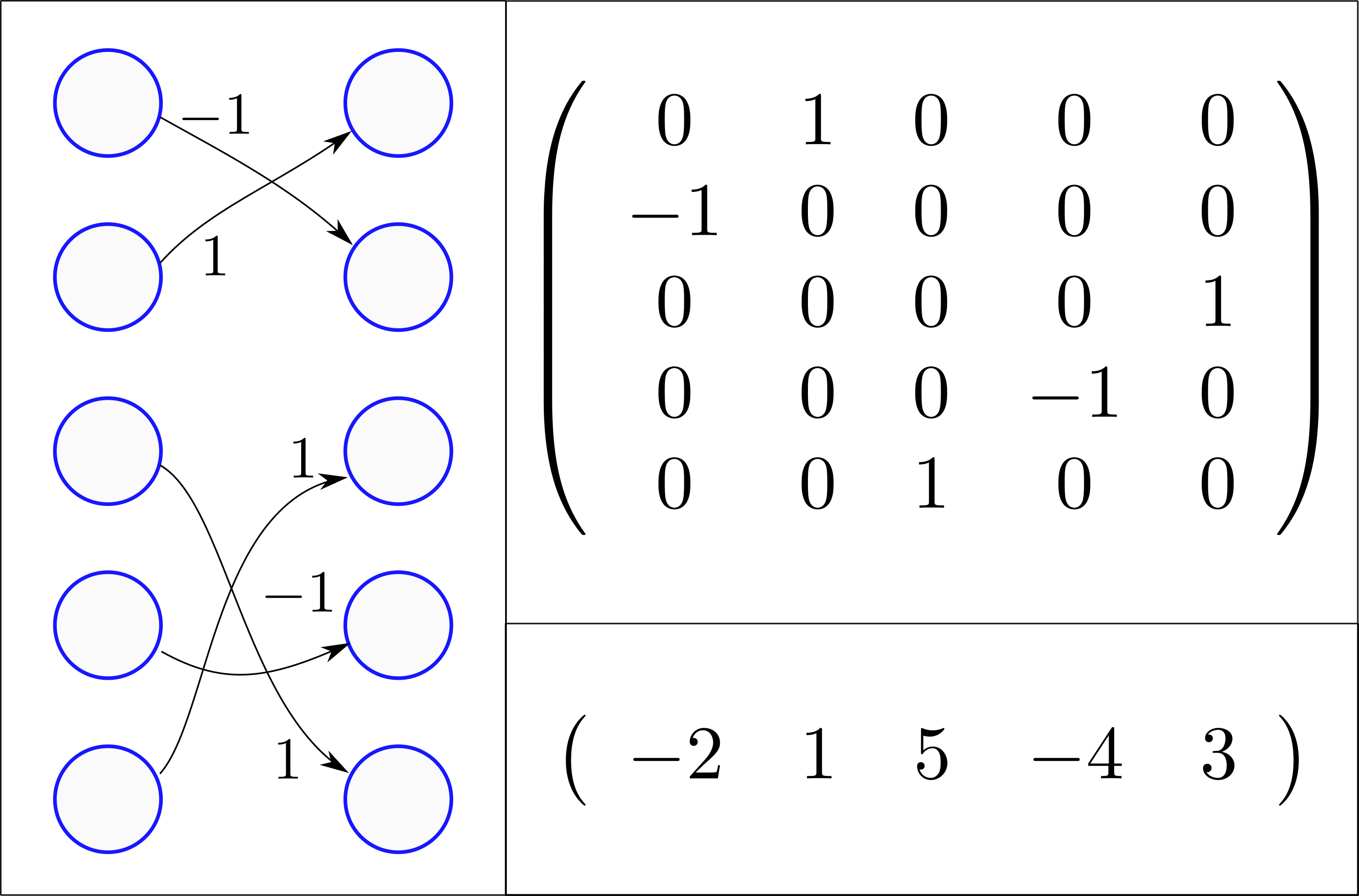
Figure 1: Different representations of an element $\sigma$ of $B_{5}$. Left: graph; Top right: Matrix notation; Bottom right: Cauchy one line notation

Even if the matrix representation looks more intuitive, for efficiency reasons, we use the Cauchy one line representation to compose the symmetries. Let us consider again the function

$$f(x_{1},x_{2})\overset{(\ref{eq:fqdex})}{=}q_{0}+q_{1}x_{1}+q_{2}x_{2}+q_{3}x_{1}^{2}+q_{4}x_{1}x_{2}+q_{5}x_{2}^{2}.$$ (5)

Take the symmetry

$$x_{1}\rightarrow\varepsilon_{1}x_{1};x_{2}\rightarrow\varepsilon_{2}x_{1}$$

where $\varepsilon_{i}\in\{-1,1\}$. With the Cauchy notation, this transformation is denoted by $\varepsilon=(\varepsilon_{1},2\varepsilon_{2})$. We have

$$\begin{array}[]{ccl}f(\varepsilon\mathbf{x})&=&q_{0}+q_{1}\varepsilon_{1}x_{1}+q_{2}\varepsilon_{2}x_{2}+q_{3}x_{1}^{2}+q_{4}\varepsilon_{1}\varepsilon_{2}x_{1}x_{2}+q_{5}x_{2}^{2}\end{array}$$ (6)

As a consequence, for each symmetry $\varepsilon=(\varepsilon_{1},2\varepsilon_{2})$, the pair

$$((\varepsilon_{1},2\varepsilon_{2}),(1,2\varepsilon_{1},3\varepsilon_{2},4,5\varepsilon_{1}\varepsilon_{2},6))$$ (7)

is conjugate. We thus get the choice function $\psi$ [9]:

$$\psi(\varepsilon_{1},2\varepsilon_{2})=(1,2\varepsilon_{1},3\varepsilon_{2},4,5\varepsilon_{1}\varepsilon_{2},6)$$ (8)

Given a symmetry $\varepsilon$, this choice function allows us to get a symmetry $\sigma$ such that $(\varepsilon,\sigma)$ is a conjugate pair.

3 Separator for the ellipse

This section proposes an optimal separator for an ellipse. This operator will be used later by a paver to compute boxes that are completely inside or outside the ellipse.

3.1 Cardinal points

We define the cardinal points as the points $(x_{1},x_{2})$ which satisfies

$$\left\{\begin{array}[]{c}f(\mathbf{x})=0\\ \frac{\partial f}{\partial x_{1}}(\mathbf{x})=0\,\text{or}\,\frac{\partial f}{\partial x_{2}}(\mathbf{x})=0\end{array}\right.$$

Generically, there exist four cardinal points. The cardinal point, painted red in Figure 2, at the top (left, bottom, right) is the North (West, South, East, respectively).

3.2 Contractor for the positive quadrant

The part of the ellipse between the North and the East is called the positive arc and is painted blue in Figure 2. The smallest box which encloses this arc is the positive quadrant.

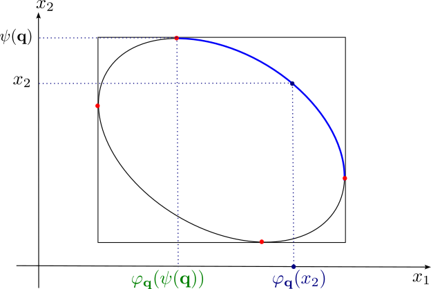
Figure 2: Positive arc and the corresponding function $\varphi_{\mathbf{q}}(x_{2})$

Proposition 1.

Take a point $x=(x_{1},x_{2})$ such that $f(\mathbf{x})=0$ of the positive quadrant. We have

$$\begin{array}[]{ccl}x_{1}&=&\varphi_{\mathbf{q}}(x_{2})\\ &=&\frac{-(q_{1}+q_{4}x_{2})\pm\sqrt{(q_{1}+q_{4}x_{2})^{2}-4q_{1}(q_{0}+q_{2}x_{2}+q_{5}x_{2}^{2})}}{2q_{3}}\end{array}$$ (9)

The largest feasible $x_{2}$ is

$$\begin{array}[]{ccc}x_{2}&=&\psi(\mathbf{q})\\ &=&\frac{-4q_{3}q_{2}+2q_{1}q_{4}+\sqrt{(4q_{3}q_{2}-2q_{1}q_{4})^{2}-4(4q_{3}q_{5}-q_{4}^{2})(4q_{3}q_{0}-q_{1}^{2})}}{8q_{3}q_{5}-2q_{4}^{2}}\end{array}$$ (10)

The North has the coordinates $\left(\varphi_{\mathbf{q}}(\psi(\mathbf{q})),\psi(\mathbf{q})\right)$.

Proof.

Assume that $x_{2}$ is known. Let us compute the possible value for $x_{1}$, if it exists. Since

$$f(x_{1},x_{2})\overset{(\ref{eq:fqdex})}{=}q_{3}x_{1}^{2}+\left(q_{1}+q_{4}x_{2}\right)x_{1}+q_{2}x_{2}+q_{0}+q_{5}x_{2}^{2},$$ (11)

we get the following discriminant:

$$\Delta_{1}=b_{1}^{2}-4a_{1}c_{1}$$ (12)

where

$$a_{1}=q_{3},\,b_{1}=q_{1}+q_{4}x_{2},\,c_{1}=q_{0}+q_{2}x_{2}+q_{5}x_{2}^{2}$$ (13)

The two solutions are

$$x_{1}=\frac{-b_{1}\pm\sqrt{\Delta_{1}}}{2a_{1}}.$$ (14)

We have thus proved corresponds (9) .

A value for $x_{2}$ yields a feasible $x_{1}$ if $\Delta_{1}\geq 0$, i.e.,

$$\begin{array}[]{clc}&b_{1}^{2}-4a_{1}c_{1}&\geq 0\\ \Leftrightarrow&-(q_{1}+q_{4}x_{2})^{2}+4q_{3}(q_{0}+q_{2}x_{2}+q_{5}x_{2}^{2})&\geq 0\\ \Leftrightarrow&(4q_{3}q_{5}-q_{4}^{2})x_{2}^{2}+(4q_{3}q_{2}-2q_{1}q_{4})x_{2}+4q_{3}q_{0}-q_{1}^{2}&\leq 0\end{array}$$

which is quadratic in $x_{2}.$ The discriminant is

$$\Delta_{2}=b_{2}^{2}-4a_{2}c_{2}$$ (15)

where

$$\begin{array}[]{ccc}a_{2}&=&4q_{3}q_{5}-q_{4}^{2}\\ b_{2}&=&4q_{3}q_{2}-2q_{1}q_{4}\\ c_{2}&=&4q_{3}q_{0}-q_{1}^{2}\end{array}$$ (16)

We thus get 10. ∎

Proposition 2.

Take a point $x=(x_{1},x_{2})$ such that $f(\mathbf{x})=0$ of the positive quadrant. We have

$$x_{2}=\varphi_{\sigma(\mathbf{q})}(x_{1})$$ (17)

where $\sigma=(1,3,2,6,5,4])$. The largest feasible $x_{1}$ is

$$\begin{array}[]{ccc}x_{1}&=&\psi(\sigma(\mathbf{q})).\end{array}$$ (18)

The East has the coordinates $\left(\psi(\sigma(\mathbf{q})),\varphi_{\sigma(\mathbf{q})}(\psi(\sigma(\mathbf{q})))\right)$.

Proof.

The symmetry which permutes $x_{1},x_{2}$ is $\sigma=(1,3,2,6,5,4])$. Indeed:

$$\begin{array}[]{ccc}f(x_{2},x_{1})&\overset{(\ref{eq:fqdex})}{=}&q_{0}+q_{1}x_{2}+q_{2}x_{1}+q_{3}x_{2}^{2}+q_{4}x_{1}x_{2}+q_{5}x_{1}^{2}\\ &=&q_{0}+q_{2}x_{1}+q_{1}x_{2}+q_{5}x_{1}^{2}+q_{4}x_{1}x_{2}+q_{3}x_{2}^{2}\end{array}$$ (19)

After application of the symmetry, Proposition 2 falls in the conditions of Proposition 1 (see Figure 3). ∎

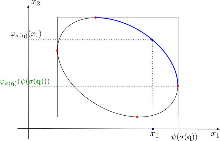
Figure 3: Positive arc and the corresponding function $\varphi_{\sigma(\mathbf{q})}$ after permutation

Proposition 3.

The smallest box which contains the North and the East is

$$[\mathbf{a}]=[\varphi_{\mathbf{q}}(\psi(\mathbf{q})),\psi(\sigma(\mathbf{q}))]\times[\varphi_{\sigma(\mathbf{q})}(\psi(\sigma(\mathbf{q}))),\psi(\mathbf{q})].$$ (20)

Proof.

The result can be read directly from Figure 4. ∎

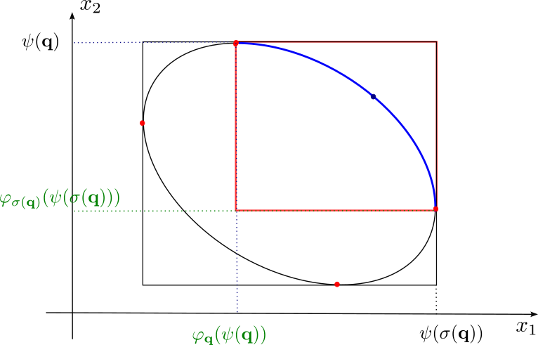
Figure 4: Smallest box which encloses the North and the East

Proposition 4.

The minimal contractor associated to the positive ellipse is

$$C_{0}^{\mathbf{q}}([\mathbf{x}])=[\mathbf{x}]\cap\left(\begin{array}[]{c}[\varphi_{\mathbf{q}}(b_{2}^{+}),\varphi_{\mathbf{q}}(b_{2}^{-})]\\ {}[\varphi_{\sigma(\mathbf{q})}(b_{1}^{+}),\varphi_{\sigma(\mathbf{q})}(b_{1}^{-})]\end{array}\right)$$ (21)

with $[\mathbf{b}]=[\mathbf{x}]\cap[\mathbf{a}].$

Proof.

This is a direct consequence of the monotonicity of the partial function $\varphi_{\mathbf{q}}$. ∎

If we apply this contractor in a paver with $\mathbf{q}=(-5,1,1,3,1,2)$, we get Figure 5.

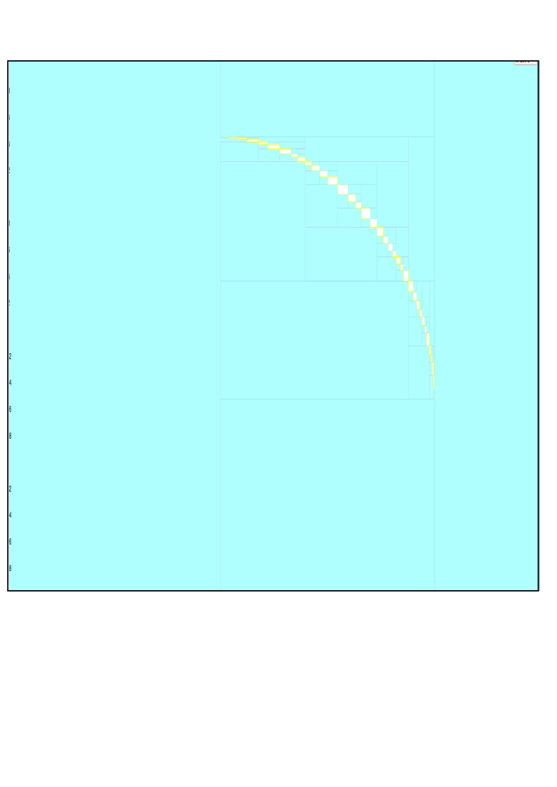
Figure 5: Illustration of the application of the contractor for the ellipse on the positive quadrant

3.3 Contractor for the ellipse boundary

Subsection 3.2 has shown how to build a contractor for the North-East quadrant of the ellipse. Recall that $C_{0}^{\mathbf{q}}([\mathbf{x}])$ contracts the box $[\mathbf{x}]$ with respect to the positive quadrant of the ellipse. It depend on the parameter vector $\mathbf{q}$ of the ellipse. Using the notion of contractor action [7], we show how we can extend this contractor $C_{0}^{\mathbf{q}}$ to other quadrants. We recall that the action of a symmetry $\varepsilon$ to the contractor $C$ is defined by

$$\varepsilon\bullet C([\mathbf{x}])=\varepsilon\circ C\circ\varepsilon^{-1}([\mathbf{x}]).$$

This means that $\varepsilon\bullet C$ is a contractor that has been built from the contractor $C$ as follows:

• Apply to the box $[\mathbf{x}]$ the symmetry $\varepsilon^{-1}$

• Apply the contractor $C$

• Apply to the resulting box $C\circ\varepsilon^{-1}([\mathbf{x}])$ the symmetry $\varepsilon$.

If we consider the pair $(\varepsilon,\sigma)$ conjugate with respect to the ellipse, the contractor $\varepsilon\bullet C_{0}^{\sigma(\mathbf{q})}$ is associated to another quadrant of the ellipse. The selection of the symmetries $(\varepsilon,\sigma)$ to be selected is made using the choice function (8). In the ellipse case, we clearly understand geometrically that 4 symmetries are needed since the ellipse has 4 quadrants (North-East, North-West, South-West, South-East). These symmetries can be computed automatically as shown in [7].

The contractor for the ellipse boundary is thus

$$[\mathbf{x}]\mapsto\bigcup_{{}^{\varepsilon\in\{(1,2),(1,-2),(-1,2),(-1,-2)\}}}(\varepsilon\bullet C_{0}^{\psi_{\varepsilon}(\mathbf{q})})([\mathbf{x}]).$$ (22)

The application of this contractor is illustrated by Figure 6.

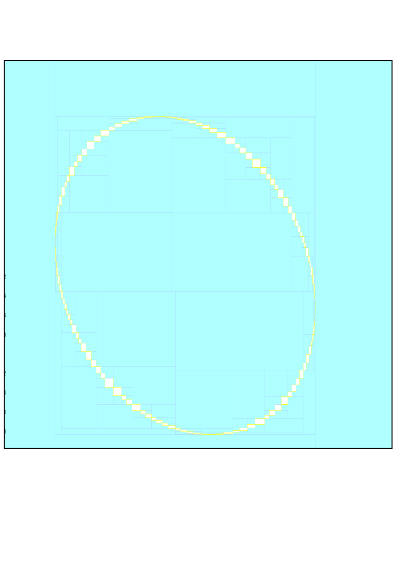
Figure 6: Illustration of the application of the contractor for the ellipse on all quadrants

3.4 Separator for the ellipse

From a contractor on the boundary of a set $\mathbb{X}$ and a test for $\mathbb{X}$, we can obtain a separator. As a consequence, we can get an inner and an outer approximations for $\mathbb{X}$ as illustrated by Figure 7.

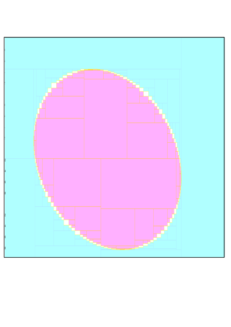
Figure 7: Illustration of the application of the separator for the ellipse on all quadrants

If we compare with a classical forward-backward contractor [2] (see 8) of other contractors such as [1] our contractor yields a more accurate approximation.

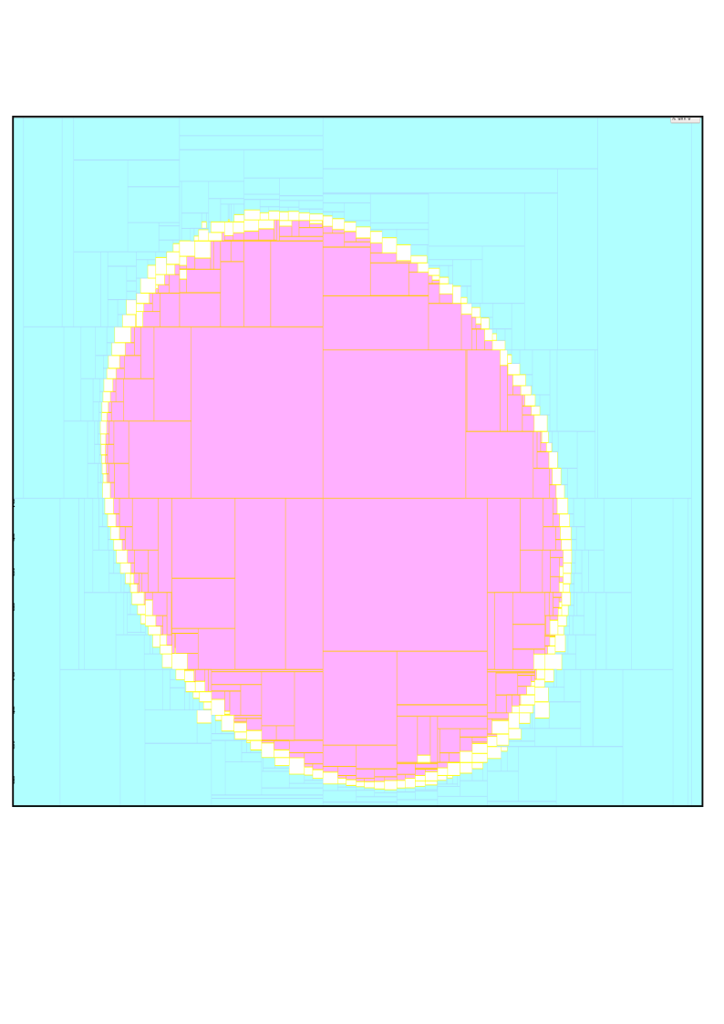
Figure 8: Classical interval contractors require a larger number of bisections

Remark. We have assumed that we had no uncertainties on $\mathbf{q}$. In case of interval uncertainty, the set to be characterized becomes

$$\mathbb{X}=\{\mathbf{x}|\exists\mathbf{q}\in[\mathbf{q}],q_{0}+q_{1}x_{1}+q_{2}x_{2}+q_{3}x_{1}^{2}+q_{4}x_{1}x_{2}+q_{5}x_{2}^{2}\leq 0\}.$$ (23)

The resolution is still possible as shown in [9].

4 Application

Interval methods have been used for localization of robots for several decades [11][16][3][5]. This section proposes to deal with a specific localization problem where the sum of distances are measured.

4.1 Ellipse

Proposition 5.

Consider two points $\mathbf{a},\mathbf{b}$ of the plane. The set $\mathbb{X}$ of all points such that

$$\|\mathbf{x}-\mathbf{a}\|+\|\mathbf{x}-\mathbf{b}\|\leq\ell$$ (24)

is an ellipse with foci points $\mathbf{a},\mathbf{b}$. The set $\mathbb{X}$ is defined by the inequality

$$\mathbf{f}_{\mathbf{a},\mathbf{b},\ell}(\mathbf{x})\leq 0$$ (25)

where

$$\mathbf{f}_{\mathbf{a},\mathbf{b},\ell}(\mathbf{x})=q_{0}+q_{1}x_{1}+q_{2}x_{2}+q_{3}x_{1}^{2}+q_{4}x_{1}x_{2}+q_{5}x_{2}^{2}$$ (26)

with

$$\begin{array}[]{ccl}q_{0}&=-&a_{1}^{4}-2a_{1}^{2}a_{2}^{2}+2a_{1}^{2}b_{1}^{2}+2a_{1}^{2}b_{2}^{2}+2a_{1}^{2}\ell^{2}\\ &&-a_{2}^{4}+2a_{2}^{2}b_{1}^{2}+2a_{2}^{2}b_{2}^{2}\\ &&+2a_{2}^{2}\ell^{2}-b_{1}^{4}-2b_{1}^{2}b_{2}^{2}+2b_{1}^{2}\ell^{2}-b_{2}^{4}+2b_{2}^{2}\ell^{2}-\ell^{4}\\ q_{1}&=&4a_{1}^{3}-4a_{1}^{2}b_{1}+4a_{1}a_{2}^{2}-4a_{1}b_{1}^{2}-4a_{1}b_{2}^{2}\\ &&-4a_{1}\ell^{2}-4a_{2}^{2}b_{1}+4b_{1}^{3}+4b_{1}b_{2}^{2}-4b_{1}\ell^{2}\\ q_{2}&=&4a_{1}^{2}a_{2}-4a_{1}^{2}b_{2}+4a_{2}^{3}-4a_{2}^{2}b_{2}-4a_{2}b_{1}^{2}\\ &&-4a_{2}b_{2}^{2}-4a_{2}\ell^{2}+4b_{1}^{2}b_{2}+4b_{2}^{3}-4b_{2}\ell^{2}\\ q_{3}&=&-4a_{1}^{2}+8a_{1}b_{1}-4b_{1}^{2}+4\ell^{2}\\ q_{4}&=&-8a_{1}a_{2}+8a_{1}b_{2}+8a_{2}b_{1}-8b_{1}b_{2}\\ q_{5}&=&-4a_{2}^{2}+8a_{2}b_{2}-4b_{2}^{2}+4\ell^{2}\end{array}$$

Proof.

We have

$$\begin{array}[]{cl}&\|\mathbf{x}-\mathbf{a}\|+\|\mathbf{x}-\mathbf{b}\|=\ell\\ \Leftrightarrow&\sqrt{(x_{1}-a_{1})^{2}+(x_{2}-a_{2})^{2}}+\sqrt{(x_{1}-b_{1})^{2}+(x_{2}-b_{2})^{2}}=\ell\end{array}$$ (27)

After some trivial symbolic calculus, we get to get rid of the square root to get

$$\begin{array}[]{ccc}4\left((x_{1}-a_{1})^{2}+(x_{2}-a_{2})^{2}\right)\left((x_{1}-b_{1})^{2}+(x_{2}-b_{2})^{2}\right)\\ -\left(\ell^{2}-(x_{1}-a_{1})^{2}-(x_{2}-a_{2})^{2}-(x_{1}-b_{1})^{2}-(x_{2}-b_{2})^{2}\right)^{2}&=&0\end{array}$$ (28)

We can develop the expression to get the coefficients of the proposition. ∎

4.2 Localization

We consider an example related to localization which can be seen as special case of interval data fitting problem [12]. Consider three sonars located at points $\mathbf{a}:(-2,1),\mathbf{b}:(-2,-1),\mathbf{c}:(3,2)$ of the plane. The emitter $\mathbf{a}$ sends a sound which is reflected by an object at position $\mathbf{x}$ received by $\mathbf{b}$ and $\mathbf{c}$ (see Figure 9). From the time of flight of the sound we want to estimate the position of the object.

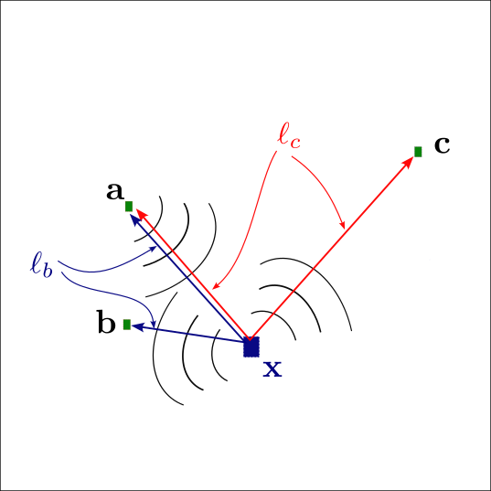
Figure 9: The sonar system returns the two distances $\ell_{b}$ and $\ell_{c}$

We assume that we were able to collect two distance intervals such that $\ell_{b}\in[4,6]$ and $\ell_{c}\in[7,9]$. The solution set $\mathbb{X}$ is defined by

$$\begin{array}[]{ccccc}\text{(i)}&&\|\mathbf{x}-\mathbf{a}\|+\|\mathbf{x}-\mathbf{b}\|&=&\ell_{b}\in[4,6]\\ \text{(ii)}&&\|\mathbf{x}-\mathbf{a}\|+\|\mathbf{x}-\mathbf{c}\|&=&\ell_{c}\in[7,9]\end{array}$$ (29)

From Proposition 5, we get that $\mathbb{X}$ is defined by

$$\mathbb{X}:\left\{\begin{array}[]{c}\mathbf{f}_{\mathbf{a},\mathbf{b},6}(\mathbf{x})\leq 0\\ \mathbf{f}_{\mathbf{a},\mathbf{b},4}(\mathbf{x})\geq 0\\ \mathbf{f}_{\mathbf{a},\mathbf{c},9}(\mathbf{x})\leq 0\\ \mathbf{f}_{\mathbf{a},\mathbf{c},7}(\mathbf{x})\geq 0\end{array}\right.$$ (30)

Using a paver, we are thus able to get in inner and an outer approximations for the set of $\mathbb{X}$ (see Figure 12).The frame box is $[-7,7]\times[-7,7].$ Figure 10 represents the inequality (10,i) and Figure 11 correspond to the inequality (10,ii). All results are guaranteed since outward rounding is implemented [14].

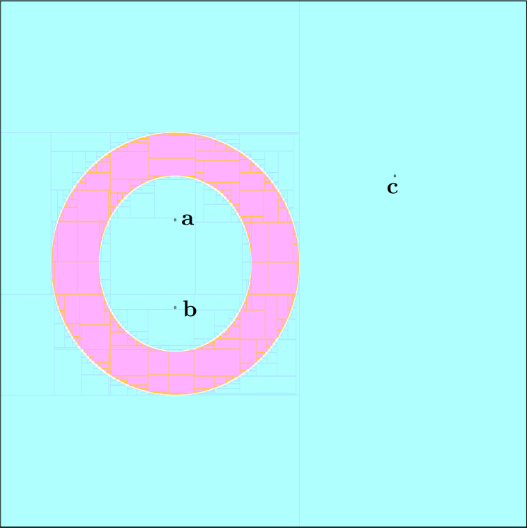
Figure 10: Set of positions consistent with the path $\mathbf{a},\mathbf{b}$

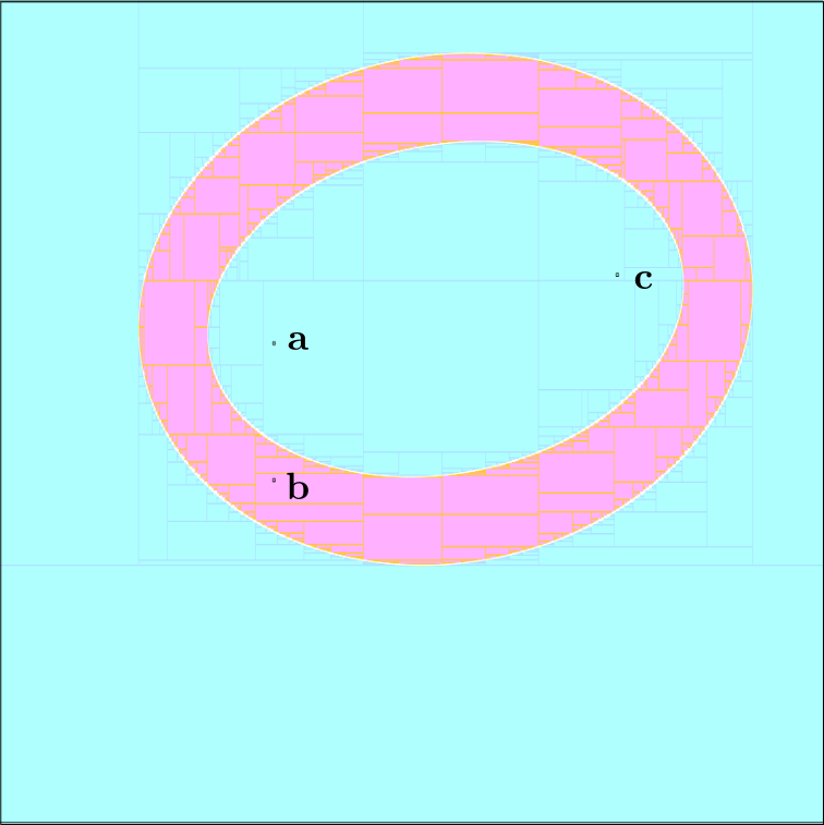
Figure 11: Set of positions consistent with the path $\mathbf{a},\mathbf{c}$

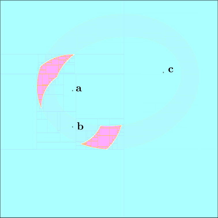
Figure 12: Set of positions consistent with the path $\mathbf{a},\mathbf{b}$ and the path $\mathbf{a},\mathbf{c}$

5 Conclusion

This paper has proposed a minimal contractor and a minimal separator for an ellipse of the plane. The notion of actions derived from hyperoctahedral symmetries allowed us to limit the analysis in on part of the constraint where the monotonicity can be assumed. The symmetries was used to extend the analysis to the whole plane.

The goal of this paper was to provide a simple example which illustrates how to use the hyperoctahedral symmetries in order to build minimal separators. Now, as shown in [9], the use of these symmetries is more interesting when we deal with projection problems where quantifier elimination is needed. This type of projection problem is indeed much more difficult to solve with classical interval approaches [6].

The Python code based on Codac [15] is given in[8].

References

- [1] I. Araya, G. Trombettoni, and B. Neveu. A contractor based on convex interval taylor. In N. Beldiceanu, N. Jussien, and E. Pinson, editors, Integration of AI and OR Techniques in Contraint Programming for Combinatorial Optimzation Problems - 9th International Conference, CPAIOR 2012, Nantes, France, May 28 - June1, 2012. Proceedings, volume 7298 of Lecture Notes in Computer Science, pages 1–16. Springer, 2012.
- [2] F. Benhamou, F. Goualard, L. Granvilliers, and J-F. Puget. Revising Hull and Box Consistency. In ICLP, pages 230–244, 1999.
- [3] E. Colle and S. Galerne. Mobile robot localization by multiangulation using set inversion. Robotics and Autonomous Systems, 61(1):39–48, 2013.
- [4] H. Coxeter. The Beauty of Geometry: Twelve Essays. Dover Books on Mathematics, 1999.
- [5] V. Drevelle and P. Bonnifait. High integrity gnss location zone characterization using interval analysis. In ION GNSS, 2009.
- [6] M. Hladík and S. Ratschan. Efficient Solution of a Class of Quantified Constraints with Quantifier Prefix Exists-Forall. Mathematics in Computer Science, 8(3-4):329–340, July 2014.
- [7] L. Jaulin. Actions of the hyperoctahedral group to compute minimal contractors. Artif. Intell., 313:103790, 2022.
- [8] L. Jaulin. Codes associated with the paper entitled: Optimal separator for an ellipse; Application to localization. www.ensta-bretagne.fr/jaulin/ctcellipse.html, 2023.
- [9] L. Jaulin. Inner and outer characterization of the projection of polynomial equations using symmetries, quotients and intervals. International Journal of Approximate Reasoning, 159:108928, 2023.
- [10] L. Jaulin and B. Desrochers. Introduction to the algebra of separators with application to path planning. Engineering Applications of Artificial Intelligence, 33:141–147, 2014.
- [11] L. Jaulin, M. Kieffer, O. Didrit, and E. Walter. Applied Interval Analysis, with Examples in Parameter and State Estimation, Robust Control and Robotics. Springer-Verlag, London, 2001.
- [12] V. Kreinovich and S. Shary. Interval methods for data fitting under uncertainty: A probabilistic treatment. Reliable Computing, 23:105–140, 2016.
- [13] R. Moore. Methods and Applications of Interval Analysis. Society for Industrial and Applied Mathematics, jan 1979.
- [14] N. Revol, L. Benet, L. Ferranti, and S. Zhilin. Testing interval arithmetic libraries, including their ieee-1788 compliance, 2022.
- [15] S. Rohou. Codac (Catalog Of Domains And Contractors), available at http://codac.io/. Robex, Lab-STICC, ENSTA-Bretagne, 2021.
- [16] S. Rohou, L. Jaulin, L. Mihaylova, F. Le Bars, and S. Veres. Reliable Robot Localization. Wiley, dec 2019.
- [17] H. Wussing. The Genesis of the Abstract Group Concept: A Contribution to the History of the Origin of Abstract Group Theory. Dover Publications, 2007.