Probing Non-Standard Neutrino Interactions with Interference: Insights from Dark Matter and Neutrino Experiments

Abstract

Neutrino-electron scattering experiments play a crucial role in investigating the non-standard interactions of neutrinos. In certain models, these interactions can include interference terms that may affect measurements. Next-generation direct detection experiments, designed primarily for dark-matter searches, are also getting sensitive to probe the neutrino properties. We utilise the data from XENONnT, a direct detection experiment, and Borexino, a low-energy solar neutrino experiment, to investigate the impact of interference on non-standard interactions. Our study considers models with an additional $U(1)$, including $U(1)_{B-L}$, $U(1)_{L_{e}-L_{\mu}}$, and $U(1)_{L_{e}-L_{\tau}}$, to investigate the impact of interference on non-standard neutrino interactions. We demonstrate that this interference can lead to a transition between the considered non-standard interaction models in the energy range relevant to both the XENONnT and Borexino experiments. This transition can be used to distinguish among the considered models if any signals are observed at direct detection or neutrino experiments. Our findings underscore the importance of accounting for the interference and incorporating both direct detection and solar neutrino experiments to gain a better understanding of neutrino interactions and properties.

1 Introduction

Currently, the investigation of neutrino properties is one of the most active fields of research in high-energy physics. Several historic milestones in neutrino physics such as supernova neutrino detection [1, 2], observations of neutrino oscillation [3, 4, 5, 6], and measurements of coherent elastic neutrino-nucleus scattering [7, 8] provide us valuable information in understanding the Standard Model (SM) of particle physics and the Universe. We can now describe how neutrinos interact with other SM particles based on the SM; however, the SM does not answer some fundamental questions about neutrinos [9, 10, 11]: e.g., neutrino mass generation and Majorana nature of neutrino. Therefore, neutrinos provide a definite pathway to search for the physics beyond the Standard Model.

In recent years, neutrino experiments [12, 13, 14, 15, 16, 17, 18, 19, 20, 21, 22, 23] and dark-matter direct detection experiments [24, 25, 26, 27, 28] have become increasingly important tools for studying the physics beyond the Standard Model [29, 30, 31, 32, 33, 34, 35, 36, 37, 38, 39, 40, 41]. Among these experiments, XENONnT [27] and Borexino [15, 16, 17] are particularly noteworthy for their sensitivity to relatively low-energy new physics.

The XENONnT [27] experiment is located in the Gran Sasso underground laboratory and its primary aim is to detect weakly interacting massive particles which are one of the most popular candidates for dark matter. However, with its $\sim 1$ keV energy threshold, XENONnT is also sensitive to elastic neutrino-electron scattering (E$\nu$ES) and can be used to study neutrino physics [41]. The experiment uses a dual-phase time projection chamber filled with liquid xenon to detect the scintillation and ionization signals produced by particles interacting with the xenon nuclei. The XENONnT experiment has recently released its blind science results with an exposure of 1.16 tonne-years and achieved background reduction by a factor of five with respect to the XENON1T experiment [25]. As a result, the well-appreciated XENON1T electron excess has been ruled out by the XENONnT experiment [27].

Borexino [14, 15, 16, 17], on the other hand, is a low-energy solar neutrino experiment also located in the Gran Sasso laboratory. Its primary goal is to study the flux and energy spectrum of solar neutrinos, which can provide valuable information about the nuclear reactions that power the Sun. Borexino uses a large liquid scintillator detector to measure the signals produced by neutrino-electron scattering.

Non-standard interactions (NSIs) are extensions to SM that introduce new interactions between neutrinos and SM particles, with important implications for neutrino oscillation experiments [42] and dark-matter direct detection experiments [28, 40, 41]. Both XENONnT and Borexino experiments are sensitive to NSIs, which can modify the neutrino-electron scattering cross-sections. However, the experiments have not yet observed any signal, providing an opportunity to constrain NSI models using their data. A key feature of NSI models is the interference terms between the SM and NSI gauge bosons, which can significantly impact the experimental results [43]. Including interference effects is crucial when studying NSI models for XENONnT and Borexino experiments because they can lead to transitions between NSI models. Therefore, if a signal is observed in these experiments, interference effects can be used to identify the underlying NSI model. It is important to mention that without interference, there would be no transitions among NSI models in the regions of interest (ROI) for these experiments.

In our study, we focus on the NSI models for E$\nu$ES namely: $U(1)_{B-L}$, $U(1)_{L_{e}-L_{\mu}}$, and $U(1)_{L_{e}-L\tau}$, which produce constructive and destructive interference (clear from Eqs. LABEL:eq:zpcont-2.5 in coherence with Table 2). We perform a detailed analysis of the behavior of these models in the context of Borexino Phase-II [17] and XENONnT [27] experiments. Our analysis show that for XENONnT the hierarchy among the NSI models persists even before and after including interference, while for Borexino a clear transition is observed among the different models. This transition among the NSI models can be particularly important to identify the specific NSI model for E$\nu$ES, that is responsible for a given signal in the experiments. In other words, if signals are observed at either the XENONnT or Borexino experiments, the interference effects could be used to determine which of the three NSI models is most likely responsible for the signals.

Overall, our study highlights the importance of considering the effects of interference when studying NSI models in the context of both neutrino and dark matter direct detection experiments. The ability to identify the specific NSI model responsible for a signal can provide valuable information for understanding the underlying physics that governs neutrino interactions with other particles.

The rest of the paper is organised as follows. In Section 2, we discuss the formalism of neutron-electron scattering. In Section 3, we describe the event rate calculation for the Borexino and XENONnT experiments. Finally, we provide our results in Section 4 and summarize our work in Section 5.

2 Formalism

In this section, we examine the NSI models, exploring the interaction of neutrinos with electrons in the presence of a low-mass gauge boson. We closely follow the notations and formalism of Ref. [44] for our presentation. The general expression of the considered models in our analysis is expressed as following,

$$-\mathcal{L}=g_{V}Q_{\ell}V_{\mu}\bar{\ell}\gamma^{\mu}\ell+g_{V}Q_{\nu_{\ell}}V_{\mu}\bar{\nu}_{\ell}\gamma^{\mu}\nu_{\ell}\,,$$ (2.1)

where $g_{V}$ is the coupling of the light gauge boson $V$ and $Q_{\ell}$, $Q_{\nu_{\ell}}$ signify the gauge charges of SM leptons and neutrinos, respectively. The corresponding differential scattering cross-section in the energy of the recoiling electron $E_{e}$ is easily available in the literature and quoted as follow,

$$\frac{d\sigma_{\nu_{l}}}{dE_{e}}=\left[\frac{d\sigma_{\rm SM}}{dE_{e}}+\frac{d\sigma_{V}}{dE_{e}}+\frac{d\sigma_{\rm int}}{dE_{e}}\,\right]_{\nu_{l}}\,,$$ (2.2)

where the first term includes the contribution from the $\nu_{l}$-$e$ scattering in the SM, while the second term corresponds to $\nu_{l}$-$e$ scattering in a NSI model. In the equation above, the interference between the SM gauge boson and the dark gauge boson is encoded in the third term. The three terms are given by [44],

$$\frac{d\sigma_{\rm SM}}{dE_{e}} = \frac{2G_{F}^{2}m_{e}}{\pi E_{\nu}^{2}}\left[c_{1}^{2}E_{\nu}^{2}+c_{2}^{2}(E_{\nu}-E_{e})^{2}-c_{1}c_{2}m_{e}E_{e}\right]\,,$$

$$\frac{d\sigma_{V}}{dE_{e}} = \frac{Q_{\nu_{\ell}}^{2}Q_{e}^{2}g_{V}^{4}m_{e}}{4\pi E_{\nu}^{2}}\frac{\left[2(E_{\nu}-E_{e})E_{\nu}+(E_{e}-m_{e})E_{e}\right]}{(2m_{e}E_{e}+m_{V}^{2})^{2}}\,,$$

$$\frac{d\sigma_{\rm int}}{dE_{e}} = \frac{Q_{\nu_{\ell}}Q_{e}g_{V}^{2}G_{F}m_{e}}{2\sqrt{2}E_{\nu}^{2}\pi(2m_{e}E_{e}+m_{V}^{2})}\times\left[c_{3}(2E_{\nu}^{2}-m_{e}E_{e})+2c_{4}(2E_{\nu}-E_{e})E_{e}\right.$$ (2.5)

$$+ \left.4s_{W}^{2}\left\{2(E_{\nu}-E_{e})E_{\nu}+(E_{e}-m_{e})E_{e}\right\}\right]\,,$$

where $G_{F}$, $E_{\nu}$, $m_{e}$, and $m_{V}$ denote the Fermi constant, the incoming neutrino energy, the electron mass, and the $V$ gauge boson mass, respectively. The neutrino flavor-dependent coefficients, $c_{1}$ through $c_{4}$, are described in Table 1. In our analysis, we consider three NSI models, namely, $U(1)_{B-L}$, $U(1)_{L_{e}-L_{\mu}}$, and $U(1)_{L_{e}-L_{\tau}}$, which correspond to the gauge charges summarized in Table 2.

Flavor	$c_{1}$	$c_{2}$	$c_{3}$	$c_{4}$
$\nu_{e}$	$s_{W}^{2}+\frac{1}{2}$	$s_{W}^{2}$	$+1$	$0$
$\nu_{\mu},\nu_{\tau}$	$s_{W}^{2}-\frac{1}{2}$	$s_{W}^{2}$	$-1$	$0$

Table 1: A summary of the coefficients in Eqs. (LABEL:eq:smcont) through (2.5). Here, $s_{W}$ represents the Weinberg angle $\theta_{W}$ as $s_{W}\equiv\sin\theta_{W}$.

Charge/Model	$U(1)_{B-L}$	$U(1)_{L_{e}-L_{\mu}}$	$U(1)_{L_{e}-L_{\tau}}$
$Q_{\nu_{e}}$	$-1$	$+1$	+1
$Q_{\nu_{\mu}}$	$-1$	$-1$	$0$
$Q_{\nu_{\tau}}$	$-1$	$0$	$-1$

Table 2: A summary of the gauge charges of the models considered in our analysis.

3 Event rate for the Borexino and XENONnT experiments

Neutrino scattering experiments can be utilised to search for light dark gauge boson. It is clear from Eqs. LABEL:eq:zpcont–2.5 that the differential cross-section increases for low recoil energy of electron and for a small value of $M_{V}$. As a result, low threshold neutrino experiments are ideal place to search for the interference effects. Borexino [14] is such an experiment we consider in our analysis, that measures the solar neutrinos [45, 17]. Specifically, we utilise the spectrum of ⁷Be monochromtic solar neutrino (with 0.862 MeV energy) measured by elastic scattering of neutrinos with liquid scintillator (doped pseudocumene). The chemical composition of pseudocumene is C₉H₁₂ with atomic mass 120.19 and 66 electrons per molecule. As a result the number of electrons in 100 tons of pseudocumene are $N_{e}=3.307\times 10^{31}$. Specifically, for our ⁷Be solar neutrino analysis, we utilise the Borexino phase-II data  with $48.3\pm 1.1$ cpd/100 tons events [17] and high-metallicity standard solar model flux, $\Phi_{{}^{7}\rm Be}=4.93\times 10^{9}$ cm^-2s^-1 [46].

The dark matter direct detection experiments have reached an unprecedented sensitivities and now are capable to explore low energy neutrino physics. In our analysis, we consider XENONnT experiment [27] with 1 keV experimental threshold which is two order of magnitude better than dedicated neutrino experiments. With an exposure of 5.9 tons, its ROI spreads between 1-30 keV. XENONnT is a dual-phase detector, looking for scintillation photons and subsequent ionisation electrons through $S_{1}$ and $S_{2}$ signals respectively, in the aftermath of a dark matter-nucleus scattering or background events. The main background in the electron recoil spectrum of XENONnT comes from $\beta$-decay events and E$\nu$ES which mainly gets contributions from $pp$ and ⁷Be (with 0.862 MeV energy) components of the solar neutrino spectrum [46]. The other components contribute negligibly to the solar neutrino spectrum.

The differential E$\nu$ES rate in considered experiments is calculated as following,

$$\frac{dR}{dE_{e}}=N_{T}\sum_{i}\int^{E^{\rm max}_{\nu}}_{E^{\rm min}_{\nu}}dE_{\nu}\frac{d\Phi^{\nu}_{i}(E_{\nu})}{E_{\nu}}\left(\frac{d\sigma_{\nu e}}{dE_{e}}P_{ee}+\sum_{f=\mu,\tau}\frac{d\sigma_{\nu f}}{dE_{e}}P_{ef}\right)\,,$$ (3.1)

where the differential cross-sections (Eqs. LABEL:eq:smcont-2.5) are weighted by the survival probabilities, arising due to neutrino propagation from the Sun to the Earth, resulting neutrino oscillations. In the equation above, $P_{ee}={\rm cos}^{4}\theta_{13}P_{eff}+{\rm sin}^{4}\theta_{13}$ is the survival probability of the solar neutrino, calculated in the two-flavour approximation, $P_{e\mu}=(1-P_{ee}){\rm cos}^{2}\theta_{23}$, and $P_{e\tau}=(1-P_{ee}){\rm sin}^{2}\theta_{23}$. Here, $P_{eff}=(1+{\rm cos2\theta_{M}}\rm{cos}2\theta_{12})$ which depends also on the neutrino propagation path and accounts for matter effects [47]. $P_{eff}$ is evaluated by taking the current best-fit values of the oscillation parameters [48] and assuming their central values for normal ordering.

In the Eq. 3.1, $N_{T}$ represents the number of target electrons; for the Borexino experiment, $N_{T}=3.307\times 10^{31}$ is the number of targets per 100 tons, while for the XENONnT experiment, $N_{T}=Z_{eff}(E_{e})m_{\rm det}N_{A}/m_{\rm Xe}$ where $m_{\rm Xe}$ is the molar mass of xenon, $m_{\rm det}$ is the fiducial mass of the detector, and $N_{A}$ is the Avogadro number. Here, $Z_{eff}(E_{e})$ represents the number of electrons that can be ionised by certain energy deposition $E_{e}$. Following [40], we approximated the latter through a series of steps functions. An alternative method is the relativistic random-phase approximation theory which improves the calculation by utilising the atomic many body effects [49]. Moreover, $\Phi_{i}^{\nu}$ represents the solar neutrino flux, which is dominated by $pp$ and ⁷Be (with 0.862 MeV energy) neutrinos in the ROI explored by the XENONnT experiment. While for the Borexino experiment, the line spectrum of ⁷Be is considered for $\Phi_{i}^{\nu}$. The minimum neutrino energy required to register the electron recoil $E_{e}$ is given by

$$E^{\rm min}_{\nu}=\frac{E_{e}+\sqrt{E^{2}_{e}+2m_{e}E_{e}}}{2}\,,$$ (3.2)

while the maximum neutrino energy $E_{\nu}^{\rm max}\sim 20$ MeV [46]. The resolution and efficiency for the XENONnT experiment are taken from [25] and [27], respectively. In the following section, we will describe our results by performing a chi-square fit to the observed data with our benchmark models.

4 Results

We constrain the new physics parameters by employing a Gaussian $\chi^{2}$ function,

$$\chi^{2}(\mathcal{S})=\sum_{k}\left(\frac{R^{k}_{\rm exp}-R^{k}_{{\rm SM}+V+B_{0}}(\mathcal{S},\beta)}{\sigma_{k}}\right)^{2}+\left(\frac{\beta^{k}}{\sigma_{\beta}^{k}}\right)^{2}\,,$$ (4.1)

where $k$ runs over the energy bins, $\sigma_{k}$ refers to statistical uncertainty per bin for a considered experiment. We consider 30 bins for our XENONnT analysis similar to the published result [27], while for Borexino we only consider ⁷Be (with 0.862 MeV energy) phase-II data in an extended energy range between 0.19-2.93 MeV [17]. In the equation above, $R^{k}_{\rm exp}$ stands for the experimental differential rate (event rate) for the XENONnT (Borexino) experiment, and $R^{k}_{{\rm SM}+V+B_{0}}(\mathcal{S},\beta)=(1+\beta)R^{k}_{{\rm SM}+V}$+$B^{k}_{0}$ where $B^{k}_{0}$ is the background reported by the relevant experiment. Here, $R^{k}_{{\rm SM}+V}$ includes the contributions from the SM and dark gauge boson, which are calculated using Eq. 3.1 for the corresponding energy bin. In our XENONnT analysis $B^{k}_{0}$ is obtained from Ref. [27] after subtracting the SM E$\nu$ES contribution, while for the Borexino experiment background is already subtracted and so we do not include any background terms in our $\chi^{2}$ model. Moreover, $\beta^{k}$ in the above equation is the penalty factor which we utilise to incorporate the uncertainty in the solar neutrino flux. In our analysis, we consider $\sigma_{\beta}^{k}=7\%$ [50, 40]. The bound on the new physics parameters is obtained by,

$$\chi^{2}-\chi^{2}_{\rm min}=2.71\,,$$ (4.2)

which corresponds to $90\%$ C.L. sensitivity reach for one degrees of freedom. We obtain our results with Eq. 4.2 for $U(1)_{B-L},U(1)_{L_{e}-L_{\mu}}$, and $U(1)_{L_{e}-L_{\tau}}$ models, while utilising the XENONnT and Borexino experiments.

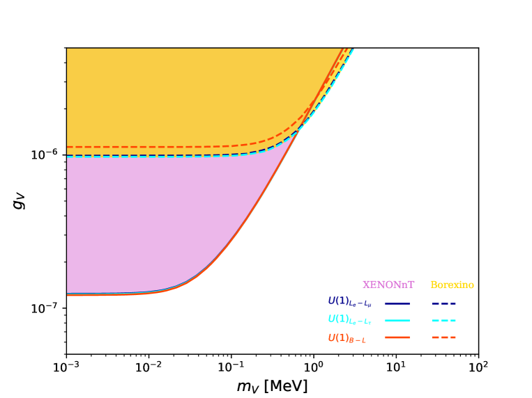
Figure 1: The exclusion limits for the $U(1)_{B-L}$, $U(1)_{L_{e}-L_{\mu}}$ and $U(1)_{L_{e}-L_{\tau}}$ models, including the interference between the SM and the dark sector, for both the XENONnT (solid lines) and Borexino (dashed lines) experiments.

In Fig. 1, we show the constrained regions by Borexino (dashed lines) and XENONnT (solid lines) in the $(m_{V},g_{V})$ plain at 90$\%$ C.L. for $U(1)_{B-L}$ (red lines), $U(1)_{L_{e}-L_{\mu}}$ (blue lines), and $U(1)_{L_{e}-L_{\tau}}$ (cyan lines) models. While obtaining the exclusion limits, we include the interference terms, due to which a hierarchy among the considered models is observed. Clearly, XENONnT [27] puts more stringent limits on the most of parameter space of the considered NSI models, surpassing the Borexino phase-II data [17]. The jiangmen underground neutrino observatory (JUNO) experiment is proposed to have a large fiducial mass of around 20 kton and excellent energy resolution of $0.03/\sqrt{E(\rm MeV)}$ [51]. This makes it capable of enhancing the sensitivity of Borexino by up to an order of magnitude. It is also important to note that the upcoming installation of the liquid scintillator-based detector (LSC) at Yamilab [52, 53] will bring significant improvements to solar neutrino measurements compared to the current Borexino experiment, which can therefore provide better sensitivities for NSI model searches.

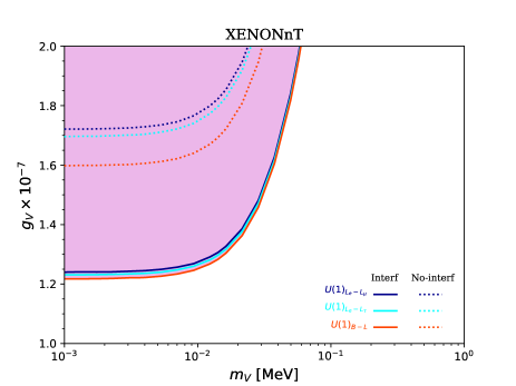
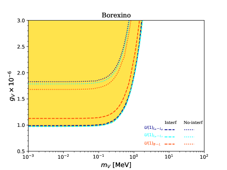
Figure 2: A zoomed version of Fig. 1 for the XENONnT (left) and Borexino (right) experiments. The solid lines represent the limits including interference, while the dotted lines show the limits excluding interference for XENONnT. For Borexino, the limits with interference are presented by the dashed lines, while the dotted lines represent the case of no-interference.

A zoomed version of Fig. 1 is depicted in Fig. 2, where the difference among NSI models is clearly appreciated for the XENONnT and Borexino experiments. For brevity, we presented exclusion limits with interference (solid lines for XENONnT and dashed lines for Borexino) and without interference (dotted lines) for the considered models. It is puzzling that in the Borexino experiment without including interference term $U(1)_{B-L}$ is the most constraining model, while inclusion of interference term leads to $U(1)_{L_{e}-L_{\tau}}$ as the most constraining model. The situation is different for the XENONnT experiment where $U(1)_{B-L}$ is always the most constraining model irrespective of interference between the SM and dark photon interaction.

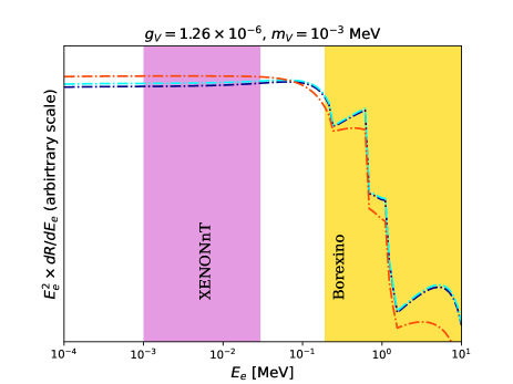
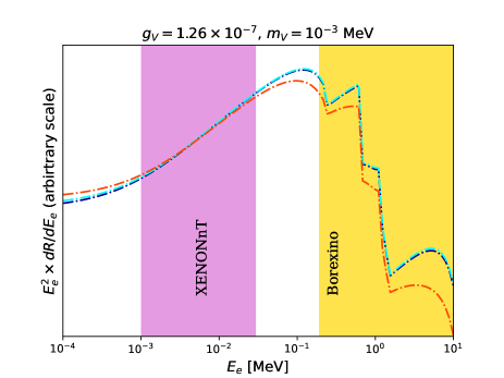
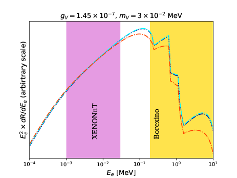
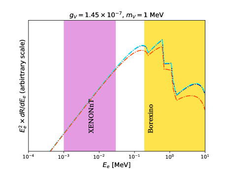
Figure 3: The differential rates in the $U(1)_{B-L}$ (red), $U_{L_{e}-L_{\mu}}$ (dark blue) and $U_{L_{e}-L_{\tau}}$ (cyan) models for the energy range relevant for Borexino and XENONnT experiments.

The solution to this conundrum is discovered in Fig. 3 where the differential rate for the considered models is shown as a function of electron recoil energy $E_{e}$. For clarity of transition behavior, we have plotted $E^{2}_{e}\times dR/dE_{e}$ instead of $dR/dE_{e}$ in Fig. 3. The shaded purple region represents the ROI for the XENONnT experiment while the shaded gold region starts from 0.190 MeV, relevant for the Borexino experiment. There are presented the results for four representative cases in variation of $g_{V}$ and $m_{V}$, for which the transition behavior can be understood utilising Eqs. LABEL:eq:zpcont-2.5. In the case of a large coupling $g_{V}$ and small mediator mass $m_{V}$, the dark photon term remains competitive with the interference term, showing a clear transition. As $g_{V}$ decrease, keeping small $m_{V}$, the transition still takes place but not as prominent. In the case of a heavy mediator and small coupling, the contribution from interference term dominates over the dark photon contribution. As a result there is no clearly visible transition for the considered model. We find that because of the interference term $U(1)_{B-L}$ is the most constraining model in the ROI of XENONnT, while $U(1)_{L_{e}-L_{\tau}}$ dominates in the region concerned to Borexino. This highlights the importance of considering the Borexino and XENONnT experiment with complimentary ROIs in our analysis. By utilising their data, it would be possible to distinguish different models.

It is important to note that regardless of the model considered, the inclusion of interference terms strengthens the exclusion limits, indicating the presence of constructive interference. In particular, the $U(1)_{B-L}$ model exhibits constructive interference for all neutrino flavors, whereas the $U(1)_{L_{e}-L_{\mu}}$ and $U(1)_{L_{e}-L_{\tau}}$ models can exhibit both constructive and destructive interference, depending on the neutrino flavor.

This phenomenon is explained by the weighted combinations of cross-sections, as described in Eq. 3.1. In the $U(1)_{B-L}$ model, the same charge ($Q_{\nu_{l}}=Q_{e}=-1$) for all neutrino flavors leads to constructive interference. In contrast, the $U(1)_{L_{e}-L_{\mu}}$ model has charges of $Q_{\nu_{e}}=Q_{e}=1$, $Q_{\nu_{\mu}}=-1$, and $Q_{\nu_{\tau}}=0$ while the $U(1)_{L_{e}-L_{\tau}}$ model has charges of $Q_{\nu_{e}}=Q_{e}=1$, $Q_{\nu_{\mu}}=0$, and $Q_{\nu_{\tau}}=-1$. As a result, $\nu_{e}$ experiences constructive interference, while $\nu_{\mu}$ or $\nu_{\tau}$ experience destructive interference in these models. Despite these variations, the dominance of the electron-neutrino scattering cross-section over the muon-neutrino and tau-neutrino scattering cross-sections leads to an overall constructive interference between the SM gauge boson and the dark gauge boson across all models.

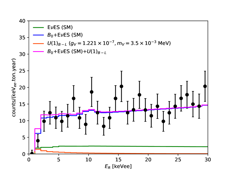
Figure 4: Expected signal from the $U(1)_{B-L}$ model and comparison with the experimental data at XENONnT [27]. Here, the black dots with the error-bar represents the XENONnT data, while $B_{0}$ is the background obtained from Ref. [27] after subtracting the SM E$\nu$ES contribution.

In Fig. 4, we show the expected signal from the $U(1)_{B-L}$ model with the background ($B_{0}$) obtained from Ref. [27] and the SM E$\nu$ES contribution, which is compared with the observed data by the XENONnT experiment [27]. The chosen benchmark is consistent with Fig. 1.

5 Summary

We studied the impact of the interference between the standard and non-standard neutrino interactions in $U(1)$-extended models while analysing the data from the XENONnT and Borexino experiments. Our study underlines a transition between different non-standard interaction models because of the presence of the interference between the standard and non-standard interactions. Depending upon the vector-mediator coupling to the SM and its mass, the hierarchy among considered models is opposite in nature for the ROIs of the XENONnT and Borexino experiments. In the epoch of observed signals at direct detection or neutrino experiments, this transition can be used to distinguish among considered NSI models. Basically, our findings underscore the importance of incorporating both direct detection and solar neutrino experiments to gain a better understanding of neutrino interactions and properties.

References

- [1] Kamiokande-II collaboration, K. Hirata et al., Observation of a Neutrino Burst from the Supernova SN 1987a, Phys. Rev. Lett. 58 (1987) 1490–1493.
- [2] R. M. Bionta et al., Observation of a Neutrino Burst in Coincidence with Supernova SN 1987a in the Large Magellanic Cloud, Phys. Rev. Lett. 58 (1987) 1494.
- [3] Super-Kamiokande collaboration, Y. Fukuda et al., Evidence for oscillation of atmospheric neutrinos, Phys. Rev. Lett. 81 (1998) 1562–1567, [hep-ex/9807003].
- [4] SNO collaboration, Q. R. Ahmad et al., Direct evidence for neutrino flavor transformation from neutral current interactions in the Sudbury Neutrino Observatory, Phys. Rev. Lett. 89 (2002) 011301, [nucl-ex/0204008].
- [5] Daya Bay collaboration, F. P. An et al., Observation of electron-antineutrino disappearance at Daya Bay, Phys. Rev. Lett. 108 (2012) 171803, [1203.1669].
- [6] RENO collaboration, J. K. Ahn et al., Observation of Reactor Electron Antineutrino Disappearance in the RENO Experiment, Phys. Rev. Lett. 108 (2012) 191802, [1204.0626].
- [7] COHERENT collaboration, D. Akimov et al., Observation of Coherent Elastic Neutrino-Nucleus Scattering, Science 357 (2017) 1123–1126, [1708.01294].
- [8] COHERENT collaboration, D. Akimov et al., First Measurement of Coherent Elastic Neutrino-Nucleus Scattering on Argon, Phys. Rev. Lett. 126 (2021) 012002, [2003.10630].
- [9] S. M. Bilenky and S. T. Petcov, Massive Neutrinos and Neutrino Oscillations, Rev. Mod. Phys. 59 (1987) 671.
- [10] J. Lesgourgues and S. Pastor, Massive neutrinos and cosmology, Phys. Rept. 429 (2006) 307–379, [astro-ph/0603494].
- [11] F. T. Avignone, III, S. R. Elliott and J. Engel, Double Beta Decay, Majorana Neutrinos, and Neutrino Mass, Rev. Mod. Phys. 80 (2008) 481–516, [0708.1033].
- [12] TEXONO collaboration, H. T. Wong et al., A Search of Neutrino Magnetic Moments with a High-Purity Germanium Detector at the Kuo-Sheng Nuclear Power Station, Phys. Rev. D 75 (2007) 012001, [hep-ex/0605006].
- [13] A. G. Beda, V. B. Brudanin, V. G. Egorov, D. V. Medvedev, V. S. Pogosov, E. A. Shevchik et al., Gemma experiment: The results of neutrino magnetic moment search, Phys. Part. Nucl. Lett. 10 (2013) 139–143.
- [14] Borexino collaboration, G. Alimonti et al., Science and technology of BOREXINO: A Real time detector for low-energy solar neutrinos, Astropart. Phys. 16 (2002) 205–234, [hep-ex/0012030].
- [15] Borexino collaboration, G. Bellini et al., Final results of Borexino Phase-I on low energy solar neutrino spectroscopy, Phys. Rev. D 89 (2014) 112007, [1308.0443].
- [16] BOREXINO collaboration, G. Bellini et al., Neutrinos from the primary proton–proton fusion process in the Sun, Nature 512 (2014) 383–386.
- [17] Borexino collaboration, M. Agostini et al., First Simultaneous Precision Spectroscopy of , 7Be, and Solar Neutrinos with Borexino Phase-II, Phys. Rev. D 100 (2019) 082004, [1707.09279].
- [18] COHERENT collaboration, D. Akimov et al., Observation of Coherent Elastic Neutrino-Nucleus Scattering, Science 357 (2017) 1123–1126, [1708.01294].
- [19] CONNIE collaboration, A. Aguilar-Arevalo et al., Search for light mediators in the low-energy data of the CONNIE reactor neutrino experiment, JHEP 04 (2020) 054, [1910.04951].
- [20] CONUS collaboration, H. Bonet et al., Constraints on elastic neutrino nucleus scattering in the fully coherent regime from the CONUS experiment, Phys. Rev. Lett. 126 (2021) 041804, [2011.00210].
- [21] CCM collaboration, A. A. Aguilar-Arevalo et al., First dark matter search results from Coherent CAPTAIN-Mills, Phys. Rev. D 106 (2022) 012001, [2105.14020].
- [22] J. Colaresi, J. I. Collar, T. W. Hossbach, C. M. Lewis and K. M. Yocum, Measurement of Coherent Elastic Neutrino-Nucleus Scattering from Reactor Antineutrinos, Phys. Rev. Lett. 129 (2022) 211802, [2202.09672].
- [23] P. Coloma, I. Esteban, M. C. Gonzalez-Garcia, L. Larizgoitia, F. Monrabal and S. Palomares-Ruiz, Bounds on new physics with data of the Dresden-II reactor experiment and COHERENT, JHEP 05 (2022) 037, [2202.10829].
- [24] XENON collaboration, E. Aprile et al., First Dark Matter Search Results from the XENON1T Experiment, Phys. Rev. Lett. 119 (2017) 181301, [1705.06655].
- [25] XENON collaboration, E. Aprile et al., Excess electronic recoil events in XENON1T, Phys. Rev. D 102 (2020) 072004, [2006.09721].
- [26] LZ collaboration, J. Aalbers et al., First Dark Matter Search Results from the LUX-ZEPLIN (LZ) Experiment, 2207.03764.
- [27] XENON collaboration, E. Aprile et al., Search for New Physics in Electronic Recoil Data from XENONnT, Phys. Rev. Lett. 129 (2022) 161805, [2207.11330].
- [28] CDEX collaboration, X. P. Geng et al., Search for exotic neutrino interactions using solar neutrinos in the CDEX-10 experiment, 2210.01604.
- [29] D. Montanino, M. Picariello and J. Pulido, Probing neutrino magnetic moment and unparticle interactions with Borexino, Phys. Rev. D 77 (2008) 093011, [0801.2643].
- [30] R. Harnik, J. Kopp and P. A. N. Machado, Exploring nu Signals in Dark Matter Detectors, JCAP 07 (2012) 026, [1202.6073].
- [31] S. K. Agarwalla, F. Lombardi and T. Takeuchi, Constraining Non-Standard Interactions of the Neutrino with Borexino, JHEP 12 (2012) 079, [1207.3492].
- [32] A. N. Khan, W. Rodejohann and X.-J. Xu, Borexino and general neutrino interactions, Phys. Rev. D 101 (2020) 055047, [1906.12102].
- [33] D. W. P. d. Amaral, D. G. Cerdeno, P. Foldenauer and E. Reid, Solar neutrino probes of the muon anomalous magnetic moment in the gauged , JHEP 12 (2020) 155, [2006.11225].
- [34] Z. Chen, T. Li and J. Liao, Constraints on general neutrino interactions with exotic fermion from neutrino-electron scattering experiments, JHEP 05 (2021) 131, [2102.09784].
- [35] Y. Jho, J.-C. Park, S. C. Park and P.-Y. Tseng, Leptonic New Force and Cosmic-ray Boosted Dark Matter for the XENON1T Excess, Phys. Lett. B 811 (2020) 135863, [2006.13910].
- [36] M. Abdullah et al., Coherent elastic neutrino-nucleus scattering: Terrestrial and astrophysical applications, 2203.07361.
- [37] P. Coloma, M. C. Gonzalez-Garcia, M. Maltoni, J. P. Pinheiro and S. Urrea, Constraining new physics with Borexino Phase-II spectral data, JHEP 07 (2022) 138, [2204.03011].
- [38] A. N. Khan, Light new physics and neutrino electromagnetic interactions in XENONnT, Phys. Lett. B 837 (2023) 137650, [2208.02144].
- [39] B. Dutta, S. Ghosh, T. Li, A. Thompson and A. Verma, Non-standard neutrino interactions in light mediator models at reactor experiments, JHEP 03 (2023) 163, [2209.13566].
- [40] M. Atzori Corona, W. M. Bonivento, M. Cadeddu, N. Cargioli and F. Dordei, New constraint on neutrino magnetic moment and neutrino millicharge from LUX-ZEPLIN dark matter search results, Phys. Rev. D 107 (2023) 053001, [2207.05036].
- [41] S. K. A., A. Majumdar, D. K. Papoulias, H. Prajapati and R. Srivastava, Implications of first LZ and XENONnT results: A comparative study of neutrino properties and light mediators, Phys. Lett. B 839 (2023) 137742, [2208.06415].
- [42] O. G. Miranda and H. Nunokawa, Non standard neutrino interactions: current status and future prospects, New J. Phys. 17 (2015) 095002, [1505.06254].
- [43] S. Bilmis, I. Turan, T. M. Aliev, M. Deniz, L. Singh and H. T. Wong, Constraints on Dark Photon from Neutrino-Electron Scattering Experiments, Phys. Rev. D 92 (2015) 033009, [1502.07763].
- [44] P. S. B. Dev, D. Kim, K. Sinha and Y. Zhang, New interference effects from light gauge bosons in neutrino-electron scattering, Phys. Rev. D 104 (2021) 075001, [2105.09309].
- [45] Borexino collaboration, C. Arpesella et al., Direct Measurement of the Be-7 Solar Neutrino Flux with 192 Days of Borexino Data, Phys. Rev. Lett. 101 (2008) 091302, [0805.3843].
- [46] D. Baxter et al., Recommended conventions for reporting results from direct dark matter searches, Eur. Phys. J. C 81 (2021) 907, [2105.00599].
- [47] S. J. Parke, Nonadiabatic Level Crossing in Resonant Neutrino Oscillations, Phys. Rev. Lett. 57 (1986) 1275–1278, [2212.06978].
- [48] P. F. de Salas, D. V. Forero, S. Gariazzo, P. Martínez-Miravé, O. Mena, C. A. Ternes et al., 2020 global reassessment of the neutrino oscillation picture, JHEP 02 (2021) 071, [2006.11237].
- [49] J.-W. Chen, H.-C. Chi, C. P. Liu and C.-P. Wu, Low-energy electronic recoil in xenon detectors by solar neutrinos, Phys. Lett. B 774 (2017) 656–661, [1610.04177].
- [50] A. Serenelli, Alive and well: a short review about standard solar models, Eur. Phys. J. A 52 (2016) 78, [1601.07179].
- [51] JUNO collaboration, F. An et al., Neutrino Physics with JUNO, J. Phys. G 43 (2016) 030401, [1507.05613].
- [52] S. H. Seo and Y. D. Kim, Dark Photon Search at Yemilab, Korea, JHEP 04 (2021) 135, [2009.11155].
- [53] J. R. Alonso et al., IsoDAR@Yemilab: A report on the technology, capabilities, and deployment, JINST 17 (2022) P09042, [2201.10040].