TACos: Learning Temporally Structured Embeddings for Few-Shot Keyword Spotting with Dynamic Time Warping

Abstract

To segment a signal into blocks to be analyzed, few-shot keyword spotting (KWS) systems often utilize a sliding window of fixed size. Because of the varying lengths of different keywords or their spoken instances, choosing the right window size is a problem: A window should be long enough to contain all necessary information needed to recognize a keyword but a longer window may contain irrelevant information such as multiple words or noise and thus makes it difficult to reliably detect on- and offsets of keywords. We propose TACos, a novel angular margin loss for deriving two-dimensional embeddings that retain temporal properties of the underlying speech signal. In experiments conducted on KWS-DailyTalk, a few-shot KWS dataset presented in this work, using these embeddings as templates for dynamic time warping is shown to outperform using other representations or a sliding window and that using time-reversed segments of the keywords during training improves the performance.

Index Terms—  keyword spotting, representation learning, angular margin loss, few-shot learning

1 Introduction

kws [1] is the task of detecting spoken instances of a few pre-defined keywords in audio recordings of possibly long duration. All other audio content should be ignored and thus keyword spotting (KWS) is inherently an open-set classification task. Additionally, for many KWS applications only very few training samples are available (few-shot classification [2]) and it is important to detect on- and offsets of detected keywords for further (manual) analysis of the content. Typical KWS applications are activating voice assistants [3, 4], searching for content in large databases [5] or monitoring audio streams such as (radio) communication transmissions [6].

Many state-of-the-art KWS systems rely on segmenting audio signals and applying a neural network to extract discriminative embeddings for each segment that can be used to detect keywords [7, 8]. For few-shot KWS, neural networks with a prototypical loss [9] are often used to learn an embedding function [10, 11, 12]. Similar approaches are used for few-shot detection of bioacoustic events [13] or sound events in general [14, 15]. Usually, a sliding window is applied to segment the signal into blocks of fixed size, in which keywords are searched. The chosen window size needs to be long enough to capture sufficient information for identifying a keyword. However, longer windows are likely to contain multiple keywords or, in case of a short keyword, too much irrelevant information thus degrading the performance. Additionally, precisely estimating on- and offsets of detected keywords is much more difficult with longer windows. Furthermore, the length of different keywords can strongly vary making it difficult to determine a suitable, fixed, window length.

In automatic speech recognition (ASR) [16], this problem is solved by using sequence-to-sequence losses such as the connectionist temporal classification loss [17]. However, training with such losses requires sufficient amounts of data making them unsuitable for a few-shot classification task. Although it is also possible to use a pre-trained ASR system [18, 19] or pre-trained ASR embeddings [20], this requires collecting many hours of training data recorded in similar acoustic environments and creates a large computational overhead. In [21], it has been proposed to save computational power by providing the network the ability to spike once a keyword is detected and immediately stop analyzing the remaining part of the input sequence. Classically, hand-crafted speech features such as human factor cepstral coefficients [22] are used as two-dimensional templates for dynamic time warping (DTW). However, the performance of these unsupervised approaches quickly degrades for very short words or in difficult acoustic conditions. It is also possible to combine multiple KWS approaches: In [23], DTW and hand-crafted speech features are used to obtain training data for a neural network-based KWS system. In our prior work [24], two-dimensional embeddings, to be used as features for DTW, are trained using a neural network applied to windowed segments of audio signals. Still, the obtained embeddings are mostly constant over time and thus many problems resulting from using a sliding window persist.

The contributions of this work are the following: First and foremost, TACos, a novel loss function for learning embeddings that also capture the temporal structure, and a DTW-based few-shot KWS system are proposed. Second, the few-shot KWS dataset KWS-DailyTalk based on the ASR dataset DailyTalk [25] is presented. In contrast to existing KWS datasets such as SpeechCommands [26], KWS-DailyTalk is an open-set classification dataset with isolated keywords as training data and complete spoken sentences as validation and test data. The proposed KWS system is shown to outperform systems using hand-crafted speech features, a sliding window or other KWS embeddings. Furthermore, it is shown that teaching the model to distinguish between regular and temporally reversed segments improves the performance.

2 Methodology

Fig. 1: Structure of the proposed KWS system. Blocks colored in blue are only used for training the system, blocks colored in yellow are only used for inference and blocks colored in red are used for training and inference.

This work is based on prior work on learning two-dimensional embeddings for KWS with DTW [24]. A KWS system using these embeddings can be divided into a frontend for pre-processing the data, a neural network for extracting embeddings, and a backend for computing scores and finding keywords using DTW. To improve the quality of the embeddings, we propose 1) TACos, a novel angular margin loss that also considers the position of a segment in a keyword, and 2) recognizing temporally reversed segments during training. In the following, each component of the KWS system will be reviewed and afterwards both proposed improvements will be presented. An overview of the resulting KWS system is depicted in Figure 1.

2.1 Review of embeddings for KWS with DTW

Frontend: First, all waveforms are converted to single-channel, normalized to an amplitude of $1$, resampled to $16\text{\,}\mathrm{kHz}$ and high-pass filtered at $50\text{\,}\mathrm{Hz}$. For the training samples containing isolated keywords, the waveforms are divided into overlapping segments with a length of $L_{\text{seg}}=$0.25\text{\,}\mathrm{s}$$ and an overlap of $\frac{L_{\text{seg}}}{5}$. During inference, a segment overlap of $\frac{256}{$16\,000\text{\,}\mathrm{Hz}$}$ is used to increase the temporal resolution of the resulting embeddings. Furthermore, samples are padded with $\big{\lfloor}\frac{L_{\text{seg}}\cdot 16000}{2}\big{\rfloor}$ zeros on both sides to ensure that the centers of the extracted segments align with their temporal position in the audio signal. Segments shorter than $L_{\text{seg}}$ are padded with zeros. From these, log-Mel magnitude spectrograms with $64$ Mel bins are extracted using an STFT with Hanning-weighted windows of size $1024$ and a hop size of $256$.

Neural network: To extract two-dimensional embeddings, the modified ResNet architecture from [24] is used. This model consists of four times two residual blocks [27], each using convolutional layers with filters of size $3\times 3$, max-pooling for the frequency dimension and dropout with a probability of $20\%$, followed by a global max-pooling operation over the frequency dimension and a dense layer without activation function. Throughout the network, the same time dimension is kept by padding appropriately and not applying temporal pooling operations. The model, without the loss function, has only $713,486$ trainable parameters. As a loss function, the AdaCos loss [28], which is an angular margin loss for classification with a dynamically adaptive scale parameter, is used to discriminate between different keywords. Additional details can be found in [24].

The network is trained for $1000$ epochs with a batch size of $32$ using Adam [29]. Most keywords have different lengths resulting in a class imbalance due to a different total number of segments for each keyword class. To handle this, random oversampling is applied. For data augmentation, Mixup [30] with a mixing coefficient drawn from a uniform distribution and SpecAugment [31] are used. During training, random segments of the background noise recordings from SpeechCommands [26] are used as an additional “no speech” class.

Backend: The backend consists of applying sub-sequence DTW [32]. All embeddings belonging to different segments of the same audio signal are combined by taking the mean of all individual frames of the time-frequency representation that overlap in time resulting in DTW templates. In a next step, cost matrices are computed by applying the pairwise cosine distance between the templates of test sentences and the templates extracted from individual training samples. We also experimented with computing Fréchet means of all templates belonging to the same keyword with the barycenter averaging (DBA) algorithm [33] but this led to worse performance than using the templates of the individual training samples. To compute accumulated cost matrices, the DTW step sizes $(2,1)$, $(1,1)$ and $(1,2)$ are used. Note that computing the accumulated cost matrices can be parallelized by sweeping diagonally over the cost matrix. In total, the presented KWS approach is much faster than real-time. For each temporal position, a warping path is calculated and the corresponding accumulated cost is normalized with respect to the path length. The negative accumulated costs serve as matching scores that can be compared to a pre-defined threshold. Scores exceeding the threshold are considered as valid detections of a keyword and the start and end positions of the corresponding paths are returned as on- and offsets, respectively. If multiple detections overlap in time, all detections are shortened such that, at each position in time, only the single detection with the highest score is kept. Detections with less than half the duration of the training sample belonging to the detected keyword are discarded.

2.2 TACos loss function

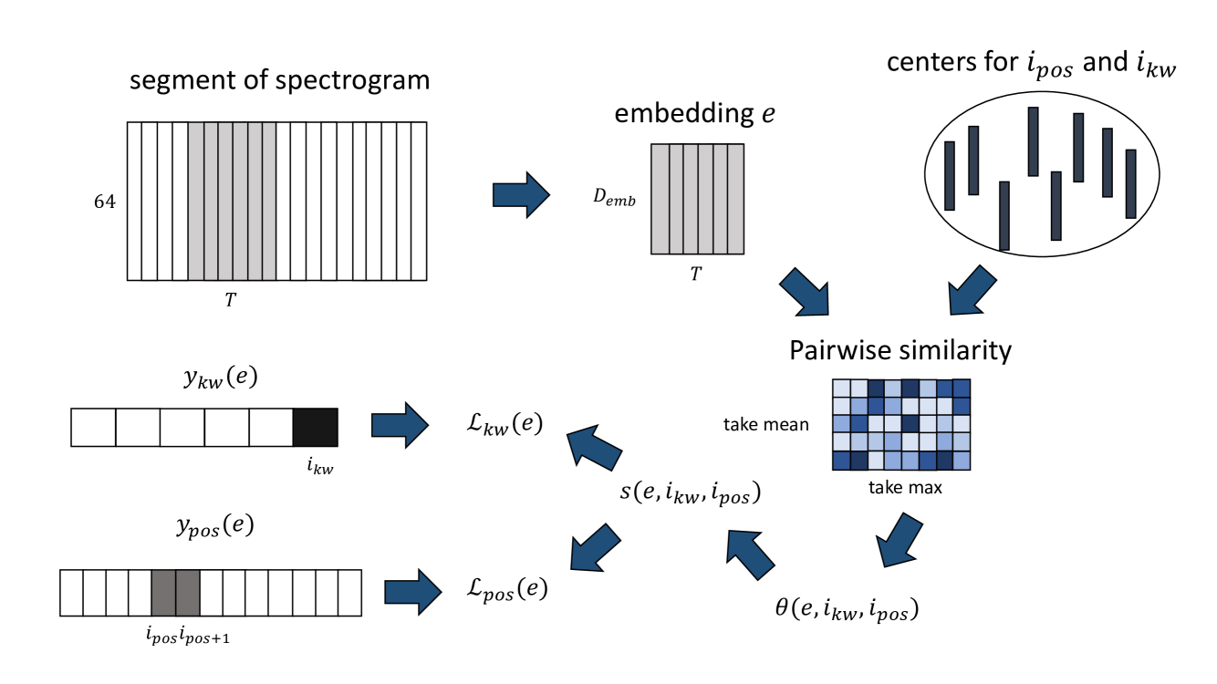
Fig. 2: Illustration of the TACos loss function.

The TACos loss function, illustated in Figure 2, consists of a supervised loss $\mathcal{L}_{\text{kw}}$ for predicting the keyword a given audio segment belongs to, which is the same loss as defined in [24], and a self-supervised loss $\mathcal{L}_{\text{pos}}$ for predicting the relative position of this segment within a keyword. When only using a supervised loss, the resulting embeddings are mostly constant over time. The idea of introducing a positional loss is to force the network to learn two-dimensional embeddings that are changing over time and thus are more suitable to be used as templates for DTW.

Since the length of different keywords may vary substantially, the absolute position of a segment within a keyword has to be encoded relative to the length of the keyword to be able to use a fixed number of position classes for all keywords. Let $K\in\mathbb{N}$ be the total number of training samples, $N_{\text{seg}}(k)\in\mathbb{N}$ denote the number of segments belonging to the $k$th training sample and define ${N_{\text{pos}}:=\max_{k\in\{1,...,K\}}\{N_{\text{seg}}(k)\}}$. Then, the relative positional encoding ${y_{\text{pos}}(e_{k,i_{\text{seg}}})\in[0,1]^{N_{\text{pos}}}}$ of embedding $e_{k,i_{\text{seg}}}$ belonging to segment $i_{\text{seg}}\in\{1,...,N_{\text{seg}}(k)\}$ of keyword sample $k$ is obtained by setting

$$y_{\text{pos}}(e_{k,i_{\text{seg}}},i_{\text{pos}})=\frac{\mathbbm{1}_{I_{\text{active}}(k,i_{\text{seg}})}(i_{\text{pos}})}{\sum_{j_{\text{pos}}=1}^{N\text{pos}}\mathbbm{1}_{I_{\text{active}}(k,i_{\text{seg}})}(j_{\text{pos}})}$$

with $I_{\text{active}}(k,i_{\text{seg}})=\big{[}1+\big{\lceil}\frac{(i_{\text{seg}}-1)\cdot N_{\text{pos}}}{N_{\text{seg}}(k)}\big{\rceil},\big{\lceil}\frac{i_{\text{seg}}\cdot N_{\text{pos}}}{N_{\text{seg}}(k)}\big{\rceil}\big{]}$. Thus, for keyword samples shorter than the longest training sample, multiple positions may be set as active with equal probability resulting in soft labels for the position.

Let $N_{\text{kw}}\in\mathbb{N}$ denote the number of different keywords in the dataset and let $y_{\text{kw}}(e,i_{\text{kw}})\in[0,1]$ denote the categorical keyword labels of the samples. Let ${T:=\big{\lceil}L_{\text{seg}}\cdot\frac{16000}{256}\big{\rceil}\in\mathbb{N}}$ be the time dimension and ${D_{\text{emb}}\in\mathbb{N}}$ be the embedding dimension of an embedding ${e\in\mathbb{R}^{T\times D_{\text{emb}}}}$ belonging to a single segment. Then, we define the cosine similarity of embedding $e$ to keyword ${i_{\text{kw}}\in\{1,...,N_{\text{kw}}\}}$ and position ${i_{\text{pos}}\in\{1,...,N_{\text{pos}}\}}$ as a temporal mean given by

$$\theta(e,i_{\text{kw}},i_{\text{pos}}):= \frac{1}{T}\sum_{t=1}^{T}\max_{i_{\text{cluster}}}\frac{\langle e(t),c(i_{\text{cluster}},i_{\text{kw}},i_{\text{pos}})\rangle}{\lVert e(t)\rVert_{2}\lVert c(i_{\text{cluster}},i_{\text{kw}},i_{\text{pos}})\rVert_{2}}$$

for trainable cluster centers $c\in\mathbb{R}^{N_{\text{cluster}}\times N_{\text{kw}}\times N_{\text{pos}}\times D_{\text{emb}}}$ with $N_{\text{cluster}}\in\mathbb{N}$, which do not have a temporal dimension. The corresponding softmax probability of embedding $e$ belonging to keyword $i_{\text{kw}}$ and position $i_{\text{pos}}$ is defined as

$$s(e,i_{\text{kw}},i_{\text{pos}}):= \frac{\exp(\hat{s}\cdot\theta(e,i_{\text{kw}},i_{\text{pos}}))}{\sum_{j_{\text{kw}=1}}^{N_{\text{kw}}}\sum_{j_{\text{pos}}=1}^{N_{\text{pos}}}\exp(\hat{s}\cdot\theta(e,j_{\text{kw}},j_{\text{pos}}))}$$

where $\hat{s}\in\mathbb{R}_{+}$ is the dynamically adaptive scale parameter as defined for the sub-cluster AdaCos loss in [34]. The probability of embedding $e$ belonging to keyword $i_{\text{kw}}$ is set to $\sum_{j_{\text{pos}}=1}^{N_{\text{pos}}}s(e,i_{\text{kw}},j_{\text{pos}})$ and the probability of embedding $e$ belonging to position $i_{\text{pos}}$ is set to $\sum_{j_{\text{kw}}=1}^{N_{\text{kw}}}s(e,j_{\text{kw}},i_{\text{pos}})$. Therefore, the loss functions for a single embedding $e$ are equal to

$$\mathcal{L}_{\text{kw}}(e) :=\sum_{i_{\text{kw}}=1}^{N_{\text{kw}}}y_{\text{kw}}(e,i_{\text{kw}})\log\big{(}\sum_{i_{\text{pos}}=1}^{N_{\text{pos}}}s(e,i_{\text{kw}},i_{\text{pos}})\big{)}$$

$$\mathcal{L}_{\text{pos}}(e) :=\sum_{i_{\text{pos}}=1}^{N_{\text{pos}}}y_{\text{pos}}(e,i_{\text{pos}})\log\big{(}\sum_{i_{\text{kw}}=1}^{N_{\text{kw}}}s(e,i_{\text{kw}},i_{\text{pos}})\big{)}$$

and the TACos loss used for training the network is

$$\mathcal{L}_{\text{TAC}} :=-\frac{1}{K}\sum_{k=1}^{K}\frac{1}{N_{\text{seg}}(k)}\sum_{i_{\text{seg}}=1}^{N_{\text{seg}}(k)}(\mathcal{L}_{\text{kw}}(e_{k,i_{\text{seg}}})+\mathcal{L}_{\text{pos}}(e_{k,i_{\text{seg}}})).$$

Note that the cluster centers $c$ significantly increase the total number of trainable parameters of the model. For all experiments in this work, ${D_{\text{emb}}=128}$ and ${N_{\text{cluster}}=16}$ were used.

2.3 Using temporally reversed segments

As a second modification, we propose to utilize temporally reversed versions of all keyword segments as additional training samples when training the embedding model. The idea is that the network has to be able to recognize the correct temporal order, i.e., we enforce that the reverse keyword is considered to be different from the non-reversed version. By doing so, the model has a harder task in correctly predicting the corresponding keyword and position of the segments. This leads to more informative embeddings and reduces the number of false detections. For each keyword class except for “no speech”, an additional unique label for the reversed keyword segments is introduced, almost doubling the number of different keyword classes. The position of the reversed segments and the segments not containing any speech are both encoded by using a uniform posterior probability over the position classes.

3 Experiments

Table 1: Event-based, micro-averaged F-score, precision and recall obtained on KWS-DailyTalk with different KWS systems. Highest F-scores for each feature representation are highlighted with bold letters, overall highest F-scores are underlined.

KWS feature representation reversed segments threshold obtained performance validation set test set F-score precision recall F-score precision recall HFCCs not applicable global 60.52% 63.25% 58.01% 56.97% 61.54% 53.04% HFCCs not applicable individual 64.71% 69.18% 60.77% 57.74% 62.58% 53.59% embeddings (sliding) not used global 39.76% 43.71% 36.46% 38.35% 41.14% 35.91% embeddings (sliding) not used individual 46.96% 49.39% 44.75% 40.44% 40.00% 40.88% embeddings (sliding) used global 44.13% 62.00% 34.25% 44.83% 59.63% 35.91% embeddings (sliding) used individual 55.43% 54.55% 56.35% 50.42% 51.14% 49.72% embeddings ($\mathcal{L}_{\text{kw}}$) [24] not used global 56.04% 52.40% 60.22% 54.25% 53.80% 54.70% embeddings ($\mathcal{L}_{\text{kw}}$) [24] not used individual 58.38% 57.14% 59.67% 53.04% 53.04% 53.04% embeddings ($\mathcal{L}_{\text{kw}}$) used global 64.58% 74.64% 56.91% 61.30% 69.72% 54.70% embeddings ($\mathcal{L}_{\text{kw}}$) used individual 66.12% 64.89% 67.40% 60.53% 57.79% 63.54% embeddings ($\mathcal{L}_{\text{kw}}+\mathcal{L}_{\text{pos}}$) not used global 62.78% 75.78% 53.59% 64.65% 82.76% 53.04% embeddings ($\mathcal{L}_{\text{kw}}+\mathcal{L}_{\text{pos}}$) not used individual 63.36% 63.19% 63.54% 63.31% 68.15% 59.12% embeddings ($\mathcal{L}_{\text{kw}}+\mathcal{L}_{\text{pos}}$) used global 65.78% 82.50% 54.70% 70.47% 89.74% 58.01% embeddings ($\mathcal{L}_{\text{kw}}+\mathcal{L}_{\text{pos}}$) used individual 69.44% 75.00% 64.64% 69.16% 79.29% 61.33%

3.1 Dataset

For all experimental evaluations, KWS-DailyTalk based on the ASR dataset DailyTalk [25] was used. KWS-DailyTalk is a five-shot KWS dataset aimed at detecting $15$ different keywords, namely “afternoon”, “airport”, “cash”, “credit card”, “deposit”, “dollar”, “evening”, “expensive”, “house”, “information”, “money”, “morning”, “night”, “visa” and “yuan”. The dataset consists of a training set with five isolated samples for each keyword and a duration of 39 seconds, as well as a validation and a test set, with an approximate duration of 10 minutes each, containing $156$ and $157$ sentences taken from dialogues, respectively. These sentences contain either none, a single, or multiple occurrences of the keywords as well as several other words that are not of interest but may cause false alarms. All keywords appear about $12$ times each in the validation and the test set. The on- and offset of each keyword were manually annotated. Furthermore, it is ensured that a keyword sample used for training and the sentences of the validation and test set that also contain this keyword do not belong to the same conversation to make the KWS task more realistic and slightly more difficult. For all experimental evaluations, the event-based F-score (micro-averaged) as implemented in the sed_eval toolbox [35] was used. All hyperparameters of the KWS systems were tuned to maximize the performance on the validation set.

3.2 Baseline approaches

For comparison, the embeddings from [24] reviewed in subsection 2.1 and the following two baseline systems are used.

HFCCs: Instead of applying sub-sequence DTW to trained embeddings, HFCCs [22, 32] based on spectrograms with a window of $40\text{\,}\mathrm{ms}$ and a step size of $10\text{\,}\mathrm{ms}$ are used. These features were shown to outperform Mel-frequency cepstral coefficients in query-by-example kws approaches. The DTW algorithm is the same as stated in subsection 2.1.

Sliding window: As a third system, a sliding window based approach using a neural network trained with the standard AdaCos loss [28] is used. The network architecture is the same as presented in subsection 2.1 with the following modifications: For each residual block, the max-pooling operation is also applied to the temporal dimension and a flattening operation is applied before projecting onto the embedding space. To detect on- and offsets of keywords, the cosine distance of the resulting embeddings to each of the keyword-specific centers is calculated first. Then, these cosine distances are compared to a pre-defined threshold and a median filter with a size equal to the average number of segments over all training samples belonging to the corresponding keyword, rounded to the nearest odd natural number, is applied to the Boolean decision results. Start and end points of the resulting positive regions are adjusted by adding $-\frac{L_{\text{seg}}}{2}$ and $+\frac{L_{\text{seg}}}{2}$, respectively, and indicate on- and offsets of detected keywords.

3.3 Experimental results

The experimental results obtained on KWS-DailyTalk can be found in Table 1. First, it can be seen that using the proposed TACos loss leads to significantly better performance than when only using $\mathcal{L}_{\text{kw}}$, as done in [24], or using a sliding window based approach, particularly so on the test set. Moreover, both embeddings perform better than HFCCs despite having only $39$ seconds of audio recordings available for training. A second major observation is that using temporally reversed segments for training the embedding model always improves the performance regardless of the chosen KWS approach. We want to emphasize that this can be observed although very powerful data augmentation techniques, namely Mixup and SpecAugment, are applied. Furthermore, tuning individual decision thresholds for each keyword class only improves the test performance when using a sliding window but not for the proposed approach for which the performance actually slightly decreases. Thus, another advantage is that one does not have to tune individual decision thresholds, which would be very impractical.

4 Conclusions

In this paper, TACos, a novel loss function for training neural networks to extract discriminative embeddings with temporal structure and a few-shot KWS-system based on DTW utilizing this loss were proposed. TACos consists of two components for learning the corresponding keyword of small speech segments as well as their relative position within a given keyword. To evaluate the performance of the KWS system, KWS-DailyTalk, an open-source dataset for few-shot keyword spotting based on DailyTalk, was presented. In experiments conducted on this dataset, it was shown that the proposed approach outperforms KWS systems based on other representations or a system using a sliding window. Last but not least, it was shown that exploiting temporally reversed segments of provided training samples improves the performance regardless of the embedding type. For future work, the proposed method will be evaluated in noisy conditions and for zero-shot KWS by pre-training the embeddings on a large ASR dataset as done in [20] and/or using pre-trained ASR embeddings instead of spectrograms as input representations.

5 Acknowledgments

The authors would like to thank Paul M. Baggenstoss, Fabian Fritz, Lukas Henneke and Frank Kurth for their valuable feedback.

References

- [1] Iván López-Espejo, Zheng-Hua Tan, John H. L. Hansen, and Jesper Jensen, “Deep spoken keyword spotting: An overview,” IEEE Access, vol. 10, pp. 4169–4199, 2022.
- [2] Yaqing Wang, Quanming Yao, James T. Kwok, and Lionel M. Ni, “Generalizing from a few examples: A survey on few-shot learning,” ACM Comput. Surv., vol. 53, no. 3, pp. 63:1–63:34, 2021.
- [3] Johan Schalkwyk, Doug Beeferman, Françoise Beaufays, Bill Byrne, Ciprian Chelba, Mike Cohen, Maryam Kamvar, and Brian Strope, ““Your word is my command”: Google search by voice: A case study,” Advances in Speech Recognition: Mobile Environments, Call Centers and Clinics, pp. 61–90, 2010.
- [4] Assaf Hurwitz Michaely, Xuedong Zhang, Gabor Simko, Carolina Parada, and Petar S. Aleksic, “Keyword spotting for google assistant using contextual speech recognition,” in ASRU. 2017, pp. 272–278, IEEE.
- [5] Ami Moyal, Vered Aharonson, Ella Tetariy, and Michal Gishri, Phonetic Search Methods for Large Speech Databases, Springer Briefs in Electrical and Computer Engineering. Springer, 2013.
- [6] Raghav Menon, Armin Saeb, Hugh Cameron, William Kibira, John A. Quinn, and Thomas Niesler, “Radio-browsing for developmental monitoring in Uganda,” in ICASSP. 2017, pp. 5795–5799, IEEE.
- [7] Herman Kamper, Weiran Wang, and Karen Livescu, “Deep convolutional acoustic word embeddings using word-pair side information,” in ICASSP. 2016, pp. 4950–4954, IEEE.
- [8] Haoxin Ma, Ye Bai, Jiangyan Yi, and Jianhua Tao, “Hypersphere embedding and additive margin for query-by-example keyword spotting,” in APSIPA ASC. 2019, pp. 868–872, IEEE.
- [9] Jake Snell, Kevin Swersky, and Richard S. Zemel, “Prototypical networks for few-shot learning,” in NeurIPS, 2017, pp. 4077–4087.
- [10] Mark Mazumder, Colby R. Banbury, Josh Meyer, Pete Warden, and Vijay Janapa Reddi, “Few-shot keyword spotting in any language,” in Interspeech. 2021, pp. 4214–4218, ISCA.
- [11] Archit Parnami and Minwoo Lee, “Few-shot keyword spotting with prototypical networks,” in ICMLT. 2022, pp. 277–283, ACM.
- [12] Byeonggeun Kim, Seunghan Yang, Inseop Chung, and Simyung Chang, “Dummy prototypical networks for few-shot open-set keyword spotting,” in Interspeech. 2022, pp. 4621–4625, ISCA.
- [13] Inês Nolasco, Shubhr Singh, E. Vidaña-Villa, E. Grout, J. Morford, M. G. Emmerson, F. H. Jensen, Ivan Kiskin, H. Whitehead, Ariana Strandburg-Peshkin, Lisa F. Gill, Hanna Pamula, Vincent Lostanlen, Veronica Morfi, and Dan Stowell, “Few-shot bioacoustic event detection at the DCASE 2022 challenge,” in DCASE, 2022, pp. 136–140.
- [14] Yu Wang, Justin Salamon, Nicholas J. Bryan, and Juan Pablo Bello, “Few-shot sound event detection,” in ICASSP. 2020, pp. 81–85, IEEE.
- [15] Yu Wang, Mark Cartwright, and Juan Pablo Bello, “Active few-shot learning for sound event detection,” in Interspeech. 2022, pp. 1551–1555, ISCA.
- [16] Jinyu Li et al., “Recent advances in end-to-end automatic speech recognition,” APSIPA Transactions on Signal and Information Processing, vol. 11, no. 1, 2022.
- [17] Alex Graves, Santiago Fernández, Faustino J. Gomez, and Jürgen Schmidhuber, “Connectionist temporal classification: labelling unsegmented sequence data with recurrent neural networks,” in ICML. 2006, pp. 369–376, ACM.
- [18] Byeonggeun Kim, Mingu Lee, Jinkyu Lee, Yeonseok Kim, and Kyuwoong Hwang, “Query-by-example on-device keyword spotting,” in ASRU. 2019, pp. 532–538, IEEE.
- [19] Li Meirong, Zhang Shaoying, Cheng Chuanxu, and Xu Wen, “Query-by-example on-device keyword spotting using convolutional recurrent neural network and connectionist temporal classification,” in ICSP, 2021, pp. 1291–1294.
- [20] R. Kirandevraj, Vinod Kumar Kurmi, Vinay P. Namboodiri, and C. V. Jawahar, “Generalized keyword spotting using ASR embeddings,” in Interspeech. 2022, pp. 126–130, ISCA.
- [21] Alan Jeffares, Qinghai Guo, Pontus Stenetorp, and Timoleon Moraitis, “Spike-inspired rank coding for fast and accurate recurrent neural networks,” in ICLR. 2022, OpenReview.net.
- [22] Dirk Von Zeddelmann, Frank Kurth, and Meinard Müller, “Perceptual audio features for unsupervised key-phrase detection,” in ICASSP. IEEE, 2010, pp. 257–260.
- [23] Raghav Menon, Herman Kamper, John A. Quinn, and Thomas Niesler, “Fast ASR-free and almost zero-resource keyword spotting using DTW and CNNs for humanitarian monitoring,” in Interspeech. 2018, pp. 2608–2612, ISCA.
- [24] Kevin Wilkinghoff, Alessia Cornaggia-Urrigshardt, and Fahrettin Gökgöz, “Two-dimensional embeddings for low-resource keyword spotting based on dynamic time warping,” in ITG Speech. 2021, pp. 9–13, VDE-Verlag.
- [25] Keon Lee, Kyumin Park, and Daeyoung Kim, “DailyTalk: Spoken dialogue dataset for conversational text-to-speech,” in ICASSP. 2023, IEEE.
- [26] Pete Warden, “Speech commands: A dataset for limited-vocabulary speech recognition,” CoRR, vol. abs/1804.03209, 2018.
- [27] Kaiming He, Xiangyu Zhang, Shaoqing Ren, and Jian Sun, “Deep residual learning for image recognition,” in CVPR. 2016, pp. 770–778, IEEE.
- [28] Xiao Zhang, Rui Zhao, Yu Qiao, Xiaogang Wang, and Hongsheng Li, “AdaCos: Adaptively scaling cosine logits for effectively learning deep face representations,” in CVPR. 2019, pp. 10823–10832, IEEE.
- [29] Diederik P. Kingma and Jimmy Ba, “Adam: A method for stochastic optimization,” in ICLR, 2015.
- [30] Hongyi Zhang, Moustapha Cisse, Yann N. Dauphin, and David Lopez-Paz, “Mixup: Beyond empirical risk minimization,” in ICLR, 2018.
- [31] Daniel S. Park, William Chan, Yu Zhang, Chung-Cheng Chiu, Barret Zoph, Ekin D. Cubuk, and Quoc V. Le, “SpecAugment: A simple data augmentation method for automatic speech recognition,” in Interspeech. 2019, pp. 2613–2617, ISCA.
- [32] Frank Kurth and Dirk von Zeddelmann, “An analysis of MFCC-like parametric audio features for keyphrase spotting applications,” in ITG Speech. 2010, VDE.
- [33] François Petitjean, Alain Ketterlin, and Pierre Gançarski, “A global averaging method for dynamic time warping, with applications to clustering,” Pattern recognition, vol. 44, no. 3, pp. 678–693, 2011.
- [34] Kevin Wilkinghoff, “Sub-cluster AdaCos: Learning representations for anomalous sound detection,” in IJCNN. 2021, IEEE.
- [35] Annamaria Mesaros, Toni Heittola, and Tuomas Virtanen, “Metrics for polyphonic sound event detection,” Applied Sciences, vol. 6, no. 6, pp. 162, 2016.