CS-TRD: a Cross Sections Tree Ring Detection method Henry Marichal1, Diego Passarella,2 Gregory Randall1 1 Instituto de Ingeniería Eléctrica, Facultad de Ingeniería, Universidad de la República, Uruguay(henry.marichal@fing.edu.uy / randall@fing.edu.uy) 2 Sede Tacuarembó, CENUR Noreste, Universidad de la República, Uruguay(diego.passarella@cut.edu.uy)

This work describes a Tree Ring Detection method for complete Cross-Sections of trees (CS-TRD). The method is based on the detection, processing, and connection of edges corresponding to the tree’s growth rings. The method depends on the parameters for the Canny Devernay edge detector ($\sigma$ and two thresholds), a resize factor, the number of rays, and the pith location. The first five parameters are fixed by default. The pith location can be marked manually or using an automatic pith detection algorithm. Besides the pith localization, the CS-TRD method is fully automated and achieves an F-Score of 89% in the UruDendro dataset (of Pinus Taeda) with a mean execution time of 17 seconds and of 97% in the Kennel dataset (of Abies Alba) with an average execution time 11 seconds.

A Python 3.11 implementation of CS-TRD is available at the web page of this article. Usage instructions are included in the README.md file of the archive. The associated online demo is accessible through the web site.

image edge detection, dendrochronology, tree ring detection

1 Introduction

Most of the available methods for dendrochronology use images taken from cores (small cylinders crossing all the tree growth rings), as opposed to complete transverse cross sections. The image analysis on cores is performed on rectangular divisions as illustrated in Figure 1. Using cores for the analysis presents some advantages. The core is a small piece of the tree, keeping it alive. The rings are measured on a small portion that can be assumed as a sequence of bands with a repetitive contrast, simplifying the image analysis. The analysis of complete sections implies the felling of the tree and, from the image analysis point of view, includes the challenge of generating a pattern of concentric closed curves that represent the tree rings. Note in the examples shown in Figure 2 that several factors make the task difficult: wood knots, fungi appearing as black spots with shapes following radial directions, and cracks that can be very wide. Some applications need the analysis of the whole cross sections, as when we are interested in studying the angular homogeneity of the ring-tree pattern. An example of such a case is when we are interested in the detection of the so-called compression wood [6] for which the lack of homogeneity in the growing pattern produces differential mechanical properties on the wood.

Several methods exist for automatically detecting tree rings in core images [18, 19, 24, 20]. As the core approach is more popular, most available datasets are of that type, and machine learning-based methods need those datasets for training. In particular, most of the machine learning-based approaches are, to the best of our knowledge, designed for core images. Core images give partial information on the tree-ring structure, which is important for some applications.

This article presents a method for detecting tree rings on images of tree cross-sections. The approach takes advantage of the knowledge of the tree cross-section’s general structure and the presence of redundant information on a radial profile for different angles around the tree’s pith.

This paper is organized as follows: Section 2 contextualizes this method with the previous work in the field. Section 3 presents the proposed automatic cross section tree-ring detection algorithm (CS-TRD). The implementation details are explained in Section 4. Section 5 briefly presents a dataset for developing and testing the proposed algorithm. Experimental results are shown in Section 6 and Section 7 concludes and discuss future work.

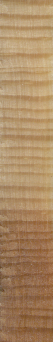
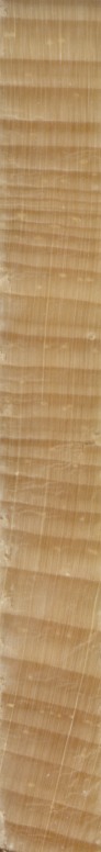
Figure 1: Examples of core tree-ring images taken from a dataset with 239 images [8].

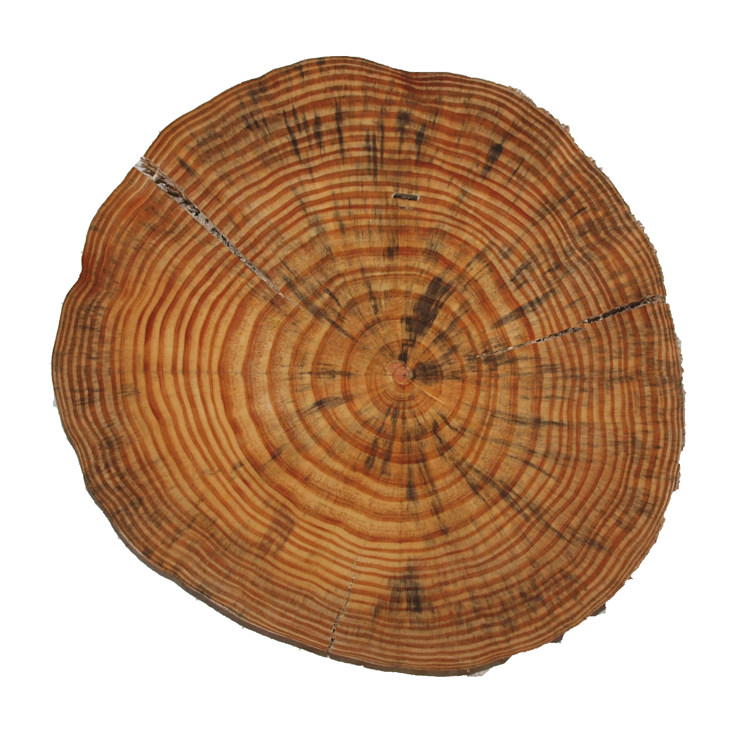
(a) F02a

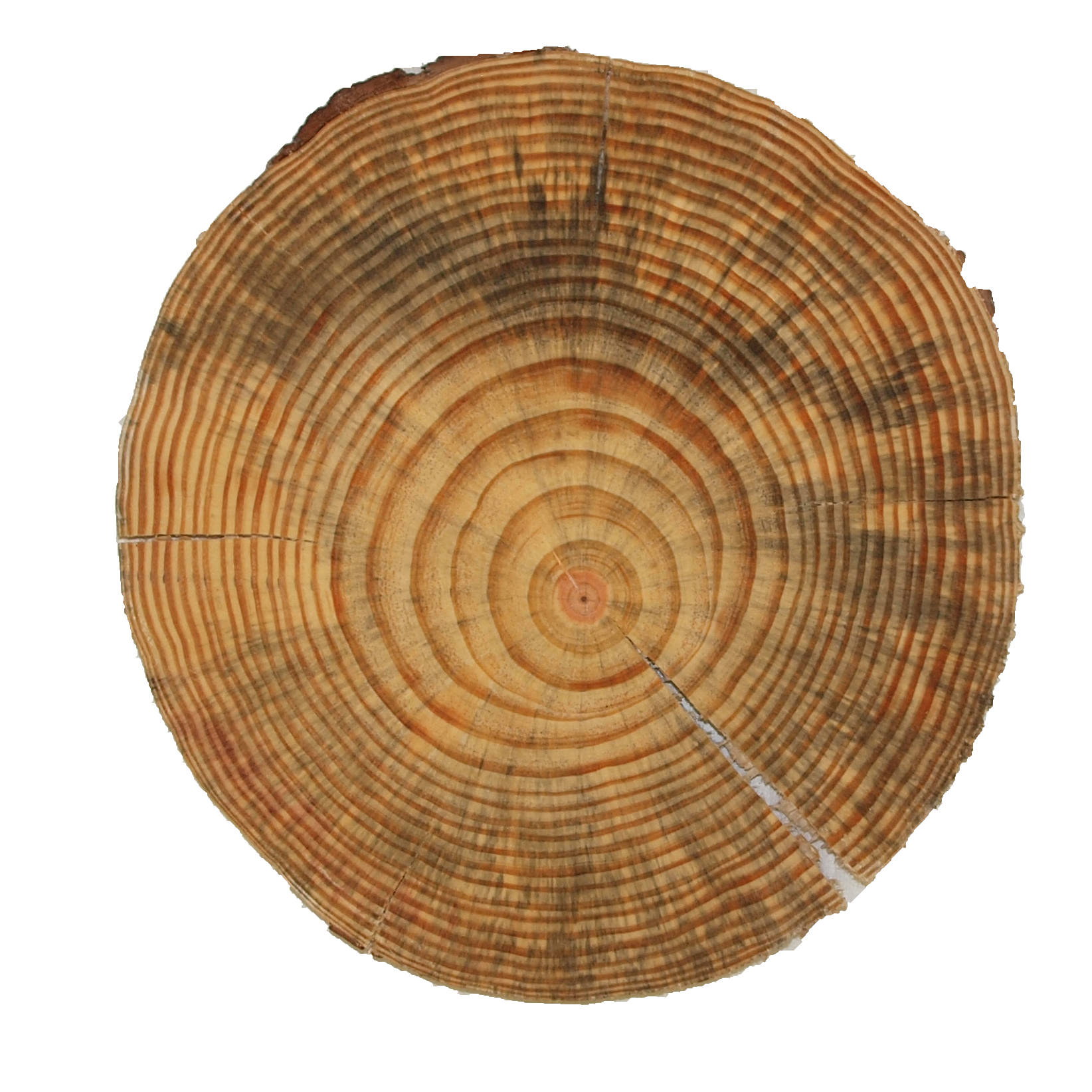
(b) F02b

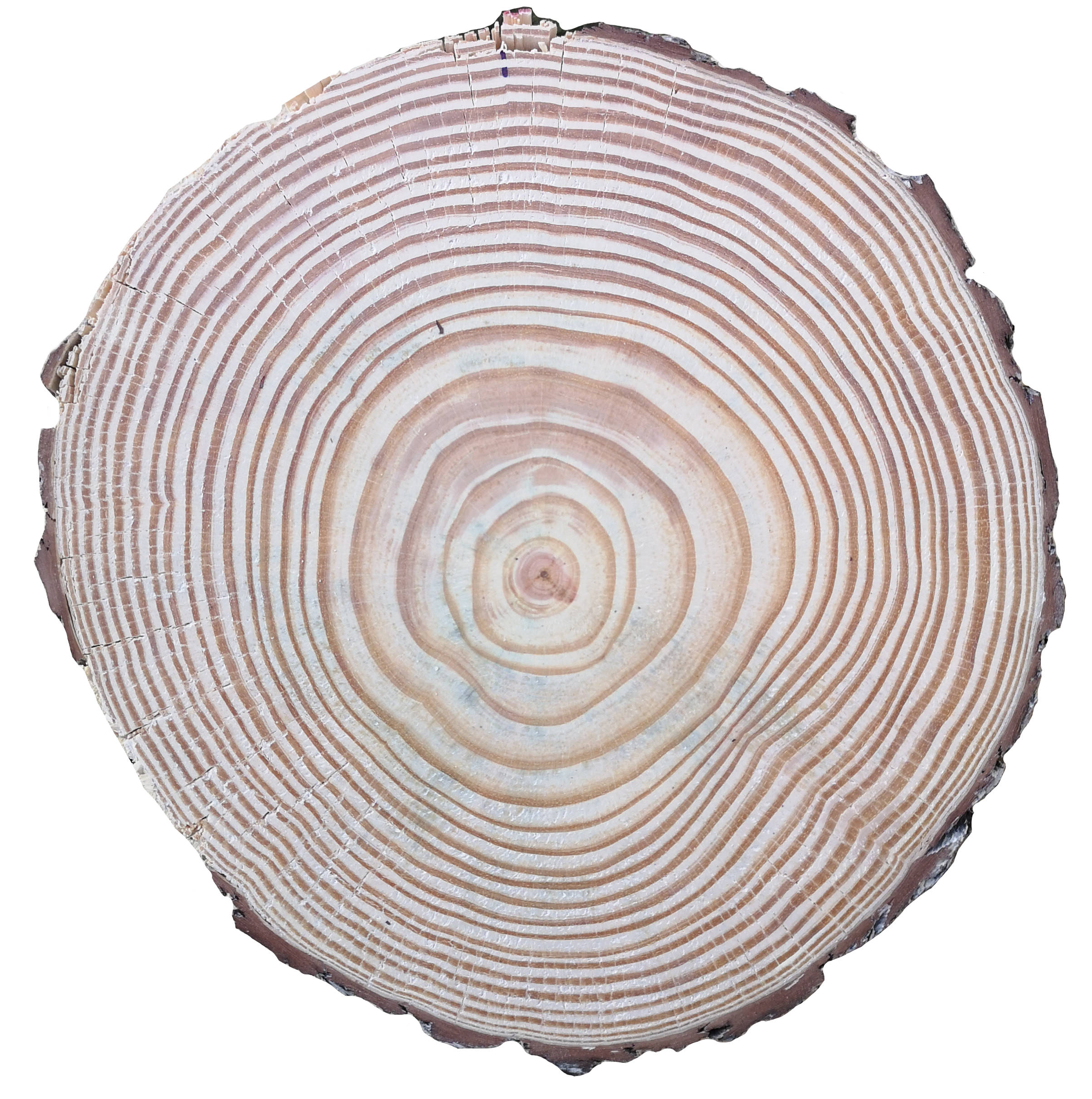
(c) F02c

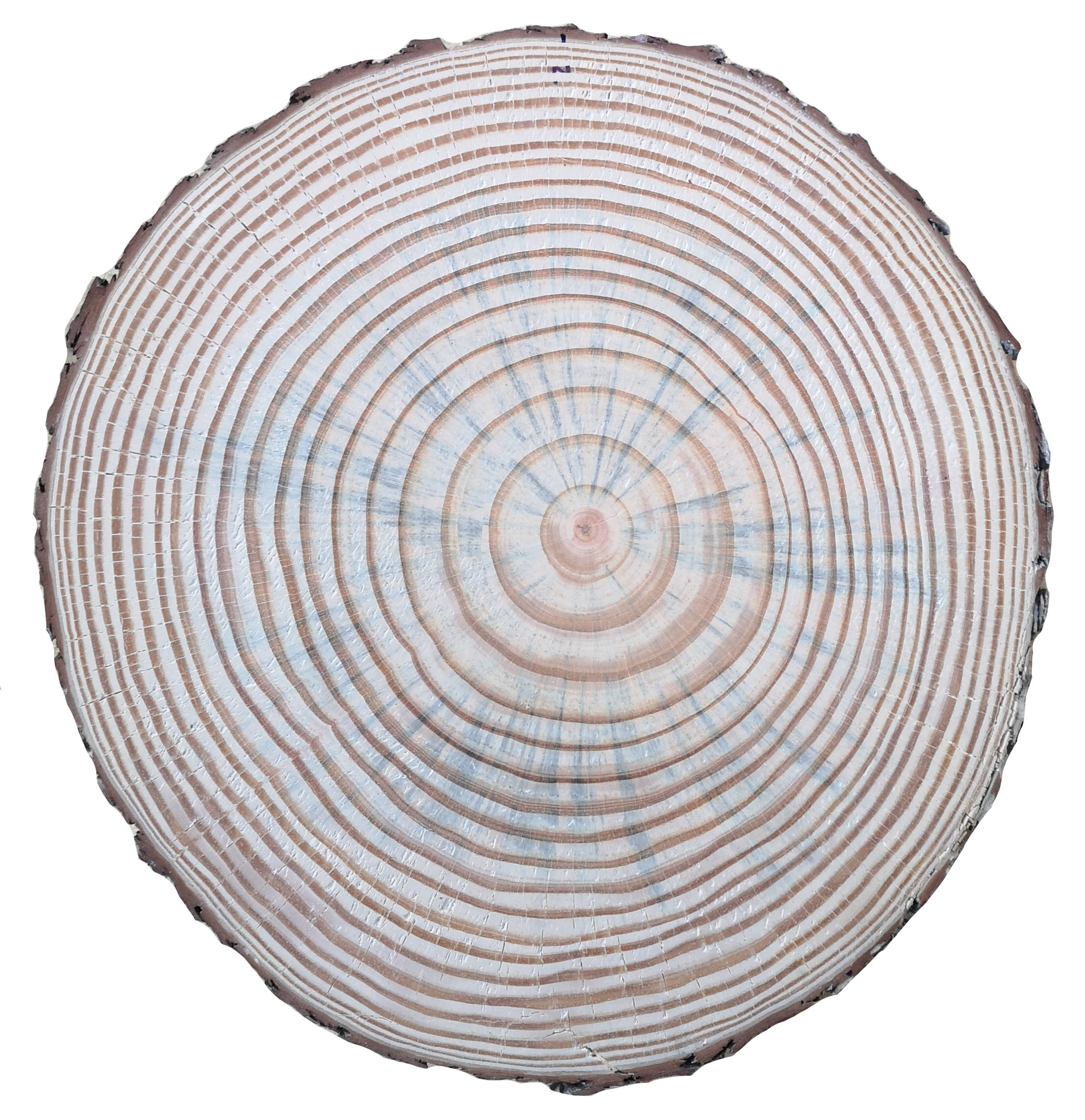
(d) F02d

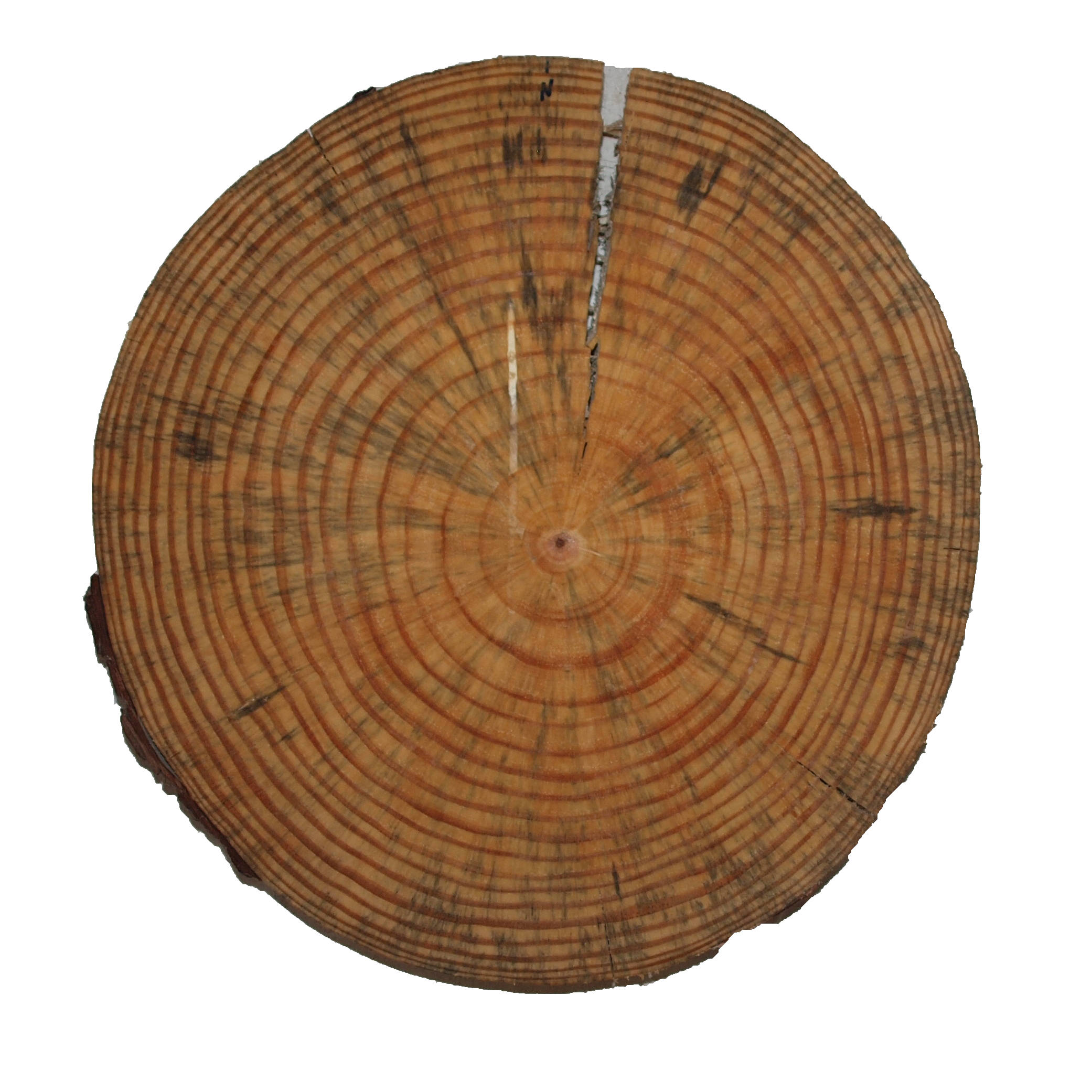
(e) F02e

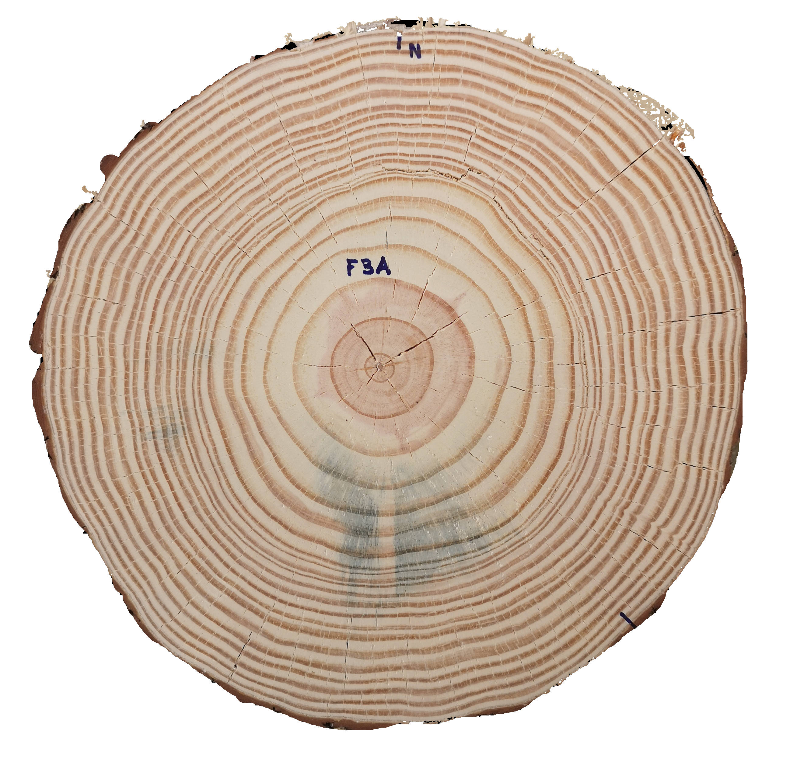
(f) F03c

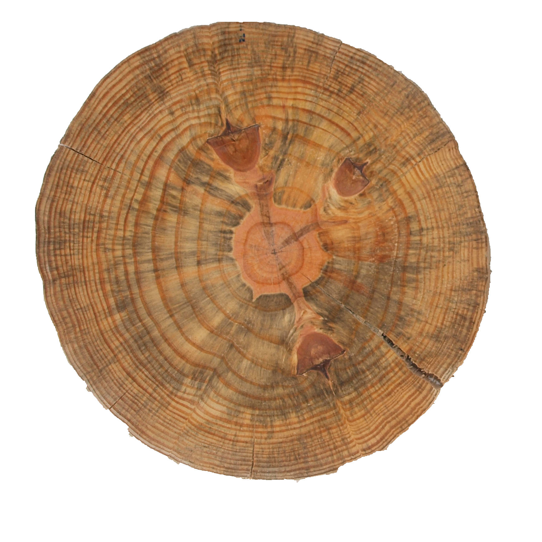
(g) F07b

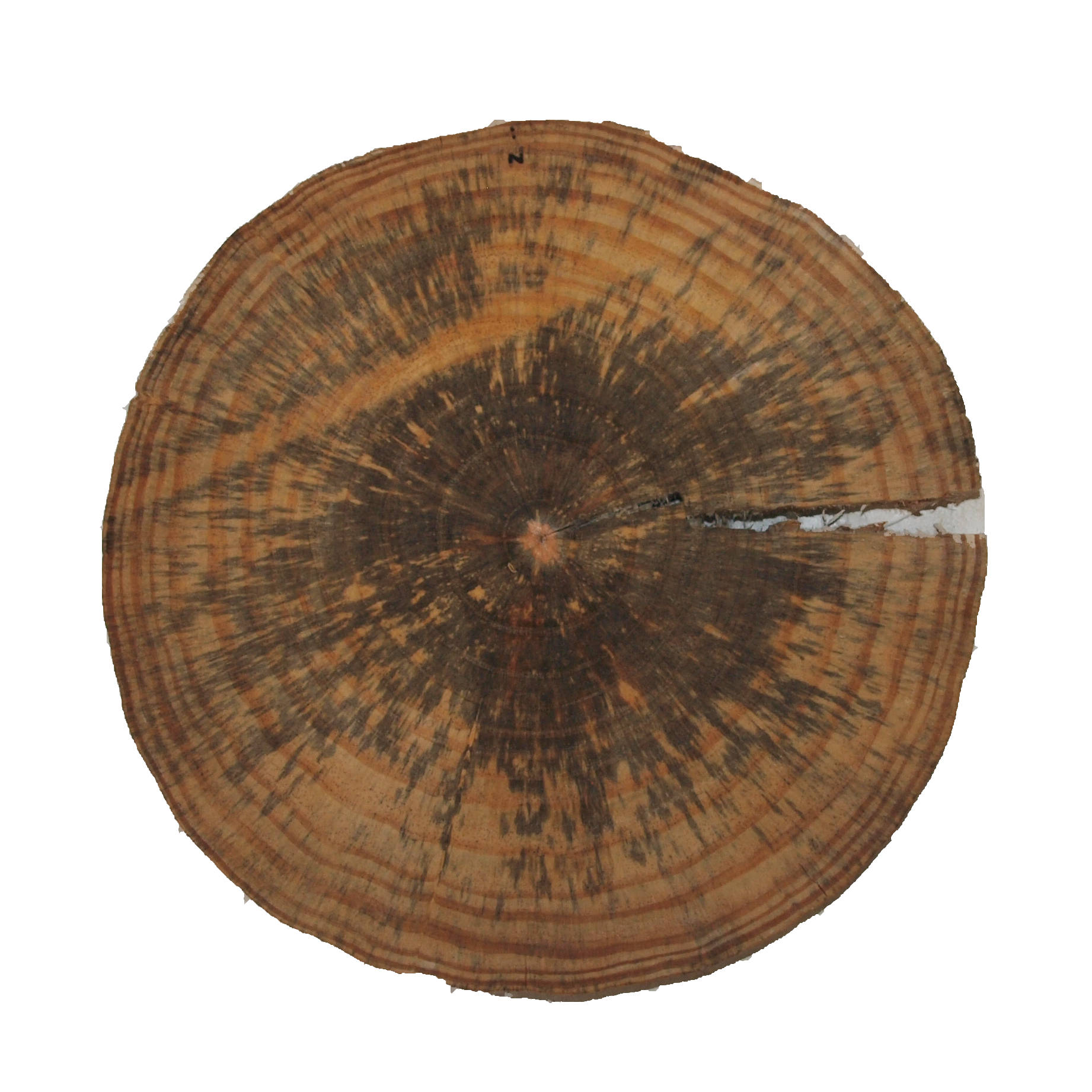
(h) L02b

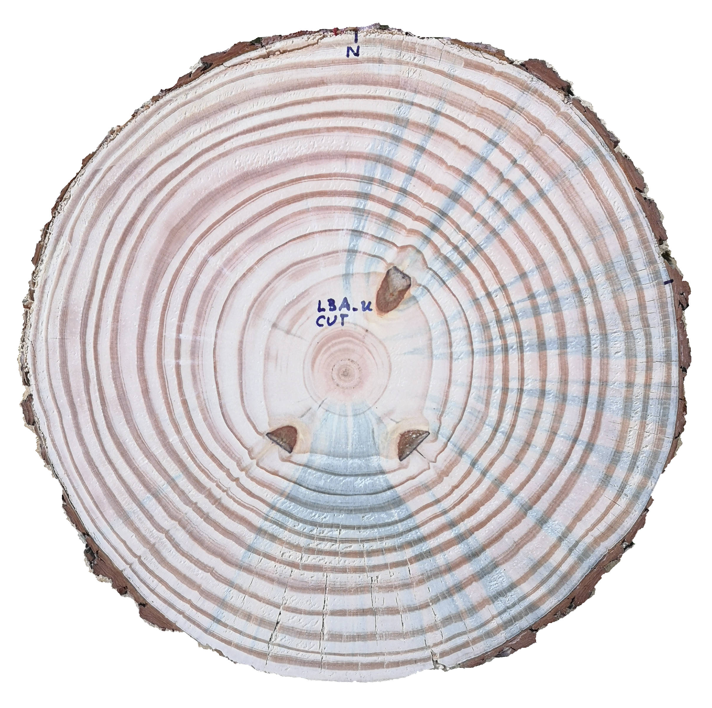
(i) L03c

Figure 2: Some examples of the images in the UruDendro dataset. Note the variability of the images and the presence of fungus (for example, in the image L02b), knots (for example, in images F07b and F03c), and cracks (for example, in images F02e and L03c). The first five images are from the same tree at different heights, as the text explains in Section 5.

2 Antecedents

Tree ring detection is an old and essential problem in forestry with multiple uses. Due to the particularity of the species of the concerned trees, many practitioners still use a manual approach, measuring the tree rings with a ruler or other (manual) tree-ring measuring system. This is a tedious and time-consuming task.

Cerda et al. [1] proposed a solution for detecting entire growth rings based on the Generalized Hough Transform. This work already suggests some general considerations that lead to the principal steps of our approach, as illustrated in Figure 4. The method was tested on ten images; neither the code nor the data are publicly available.

Norell [18] proposes a method to automatically compute the number of annual rings in end faces acquired in sawmill environments. The method applies the Grey Weighted Polar Distance Transform[19] to a rectangular section (core) that includes the pith and avoids knots or other disturbances. Norell used 24 images for training and 20 for testing its method, but the images are neither publicly available nor the method’s code.

Zhou et al. [24] proposed a method based on the traditionally manual approach, i.e., tracing two perpendicular lines across the slice and counting the peaks using a watershed-based method. They show results on five discs. Neither the algorithm nor the data are available.

Henkel et al. [11] propose a semiautomatic method for detecting tree rings on full tree cross sections using an Active Contours approach. The authors report good results on several examples, but neither the data nor the algorithm is available.

Kennel et al. [13] uses the Dual-Tree Complex Wavelet Transform[14] as part of an active contour approach. This method, which works in the entire cross-section of the tree, gives very good results on a set of 7 publicly available images. We call it the Kennel dataset and try our method on it in this work in order to compare our results with the ones reported by the authors on those images. To the best of our knowledge, the code is unavailable, so it is impossible to see how it works with our data.

Makela et al. [15] proposed an automatic method based on Jacobi Sets for the location of the pith and the ring detection on full cross-sections of trees. Neither the code nor the data are publicly available.

Fabijańska et al. [8] proposed a fully automatic image-based approach for detecting tree rings over cores images. The method is based on image gradient peak detecting and linking and is applied over a dataset with three wood species representing the ring-porous species. The same authors also proposed a deep convolutional neural network for detecting tree-rings over cores images in [7]. Comparing both methods, they reported a precision of 43% and a recall of 51% for the classical approach and a precision of 97%, and a recall of 96% for the deep learning approach. Neither the code nor the data are publicly available.

In a recent work, Polek et al.[20] uses a machine learning-based approach for automatically detecting tree rings of coniferous species but, as most of the reviewed results, work on cores instead of the whole cross-section. This is the most comprehensive approach, and most algorithms and manual protocols use this type of image input. But if the aim is to detect compressed wood, we must mark the whole cross-section to study the asymmetries between rings.

Gillert et al, [9] proposed a method for tree-ring detection over the whole cross-section but applied to microscopy images. They apply a deep learning approach using an Iterative Next Boundary Detection Network, trained and tested with microscopy images.

There exist several dendrochronology commercially available software packages. Some consist of a set of tools that help the practitioners to trace the rings manually. Others are semiautomatic, including image-processing tools to propose the ring limits. The performance generally varies significantly with certain wood anatomical features linked to wood species, climate, etc. For example, MtreeRing [22] is built using the R statistical language. It uses mathematical morphology for noise reduction and includes several methods for helping in the detection of rings (watershed-based segmentation, Canny edge detector). Like many other algorithms, it proposes an interactive tool for manual marking. To the best of our knowledge, the code is not publicly available. The CooRecorder [17] is another software application of this class, with several tools to help practitioners in the dendrochronological task, for example, to precisely determine the earlywood-latewood limits, using a zoom visualization and interactive tools. All of these packages work on cores instead of the whole disc. Constantz et al., [3] develop a tool for measuring S. Paniculatum rings. Their software measures trace by constructing transects and the rings’ areas. The input for this method is a sketch image in SVG format, with some information about the center and the rings represented by polylines, produced with Adobe Illustrator.

3 Approach

Our tree-ring detection algorithm, called CS-TRD for Cross-Section Tree-Ring Detector, is heavily based on some structural characteristics of the problem:

• The use of the whole horizontal cross-section of a tree (slice) instead of a wood dowel (or core), as most dendrochronology approaches do.

• The following properties generally define the rings on a slice:

  1. The rings are roughly concentric, even if their shape is irregular. This means that two rings can’t cross.

  2. Several rays can be traced outwards from the slice pith. Those rays will cross each ring only once.

  3. We are interested only in the rings corresponding to the latewood to early wood transitions, namely the annual rings.

3.1 Definitions

To explain the approach, we need some naming definitions; see Figure 3. We call spider web the global structure of the tree-rings we are searching for, which is depicted in a general way in Figure 3(a). It comprises a center, associated with the slice pith, which is the origin of a certain number of rays. The rings are concentric and closed curves that don’t cross each other. Each ring is formed by a curve of connected points. Each ray crosses a curve only once. The rings can be viewed as a flexible curve of points with nodes in the intersection with the rays. A chain is a set of connected nodes. As Figure 3(c) illustrates, a curve is a set of chained nodes (small green dots in the figure, noted $P_{i}$). Depending on the position of the curve concerning the center, some of those points are nodes (bigger black dots in the figure, denoted $N_{i}$ hereafter). The node can move along a ray in a radial direction, but the movement of a node in a tangential direction over the chain is forbidden. In other words, nodes can move along a ray as if it were hoops sliding along the rays. The bigger the number $Nr$ of rays, the better precision of the reconstruction of the rings. We fix $Nr=360$. Note that this is the ideal setting. In real images, rings can disappear without forming a closed curve, cells can have very varied shapes, given the deformation of the rings, undetected chains, etc.

Figure 3(c), illustrate the nomenclature used in this paper: Chains $Ch_{k}$ and $Ch_{k+1}$, intersect the rays $R_{m-1}$, $R_{m}$ and $R_{m+1}$ in nodes $N_{i-1}$, $N_{i}$ and $N_{i+1}$. Those rays and chains (as well as the four corresponding nodes) define cells $C_{l-1}$, $C_{l}$ and $C_{l+1}$. In general, a cell is limited by four nodes, but sometimes that is not the case. For example, when a chain doesn’t complete a ring or is not well detected.

During the detection process, the algorithm uses this terminology to work. We talk of chains that merge to form a ring, of rays that determine a sampling of the curve, forming chains, of the distribution of a particular measure on the cells produced by a given set of chains and rays, etc.

(a)

(b)

(c)

Figure 3: (a) The whole structure, called spider web, is formed by a center (which corresponds to the slice pith), $Nr$ rays (in the drawing $Nr=18$) and the rings (concentric curves). In the scheme, the rings are circles, but in practice, they can be (strongly) deformed as long as they don’t intersect another ring. Each ray intersects a ring only once in a point called node. The area limited by two consecutive rays and two consecutive rings is named a cell. (b) A curve is a set of connected points (small green dots). Some of those points are the intersection with rays, named nodes (black dots). A chain is a set of connected nodes. In this case, the node $N_{i}$ is the point $p_{n}$. (c) Each Chain $Ch_{k}$ and $Ch_{k+1}$, intersect the rays $R_{m-1}$, $R_{m}$ and $R_{m+1}$ in nodes $N_{i-1}$, $N_{i}$ and $N_{i+1}$. Those rays and chains (as well as the four corresponding nodes) determines cells $C_{l-1}$, $C_{l}$ and $C_{l+1}$.

3.2 Method

Figure 4 illustrates the intermediate results of the proposed method described by Algorithm 1. The input has to be an image of a tree slice without background. To subtract the background, many methods can be used. We apply a deep learning-based approach [21] based on two-level nested U-structures ($U^{2}Net$). Figure 5 shows an example of such a procedure.

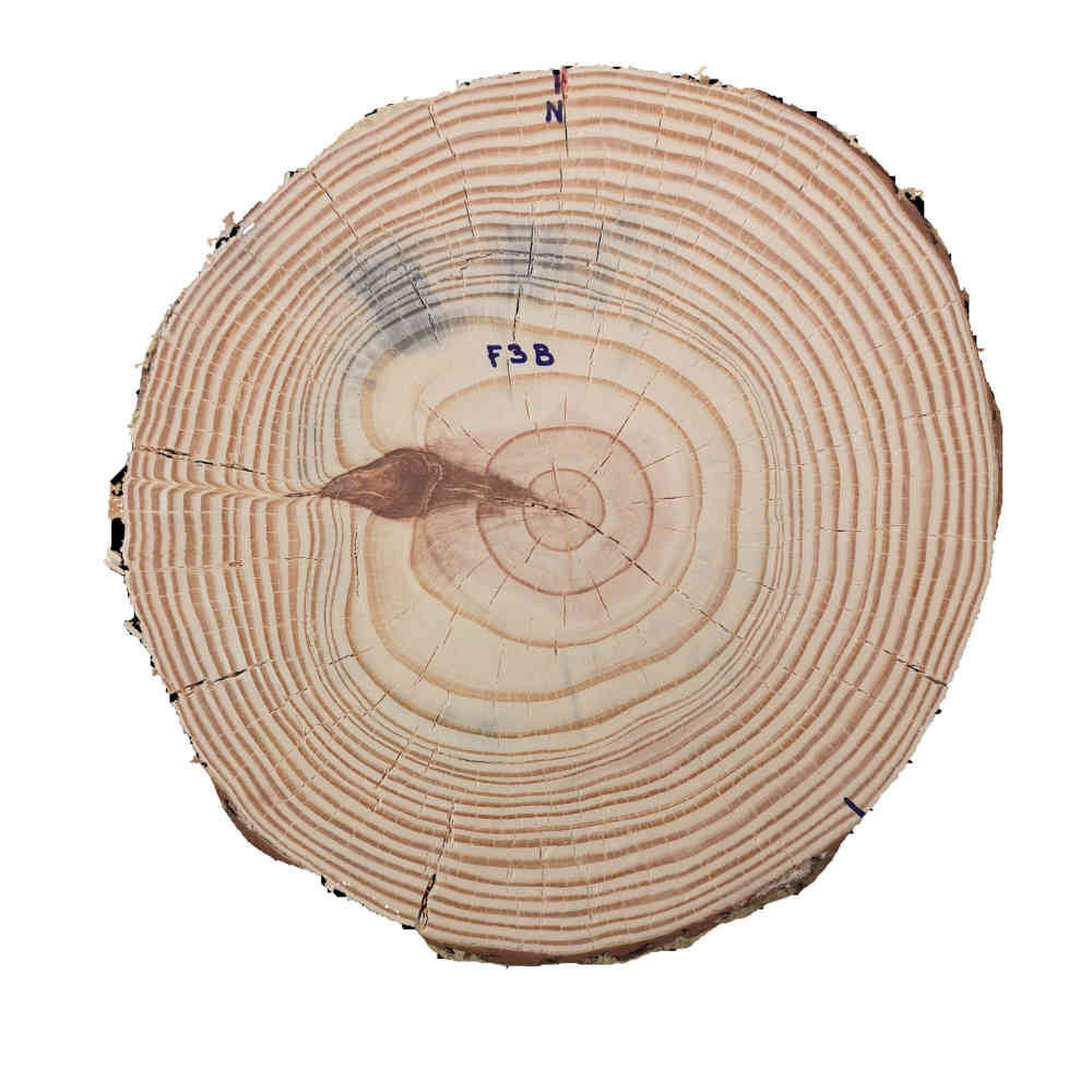
(a)

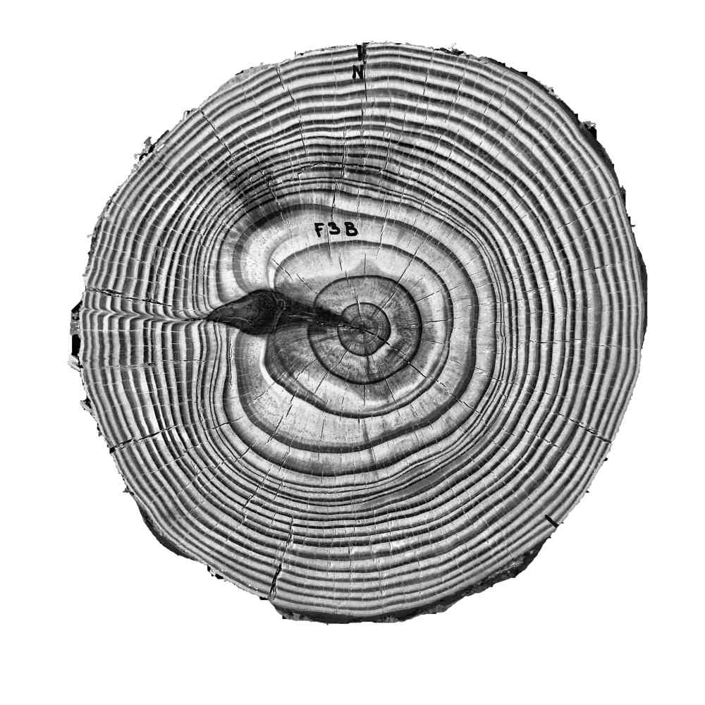
(b)

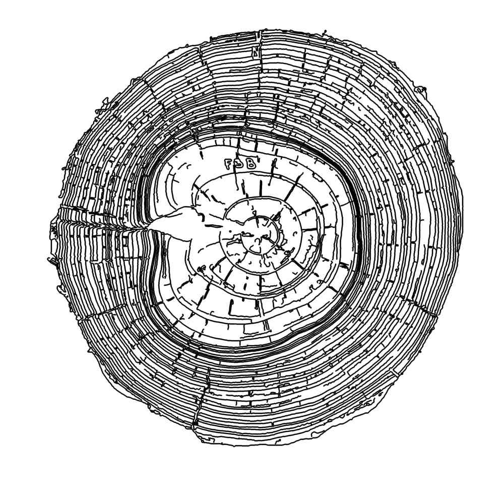
(c)

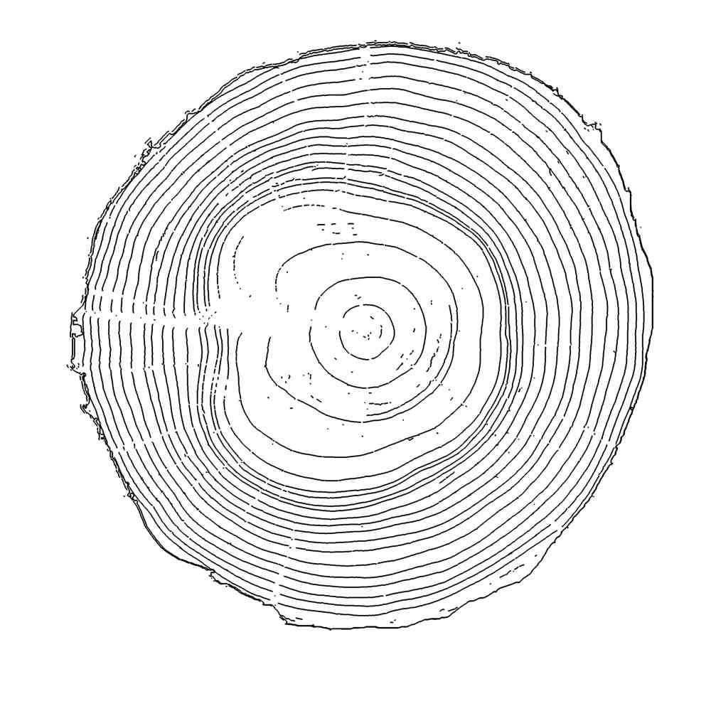
(d)

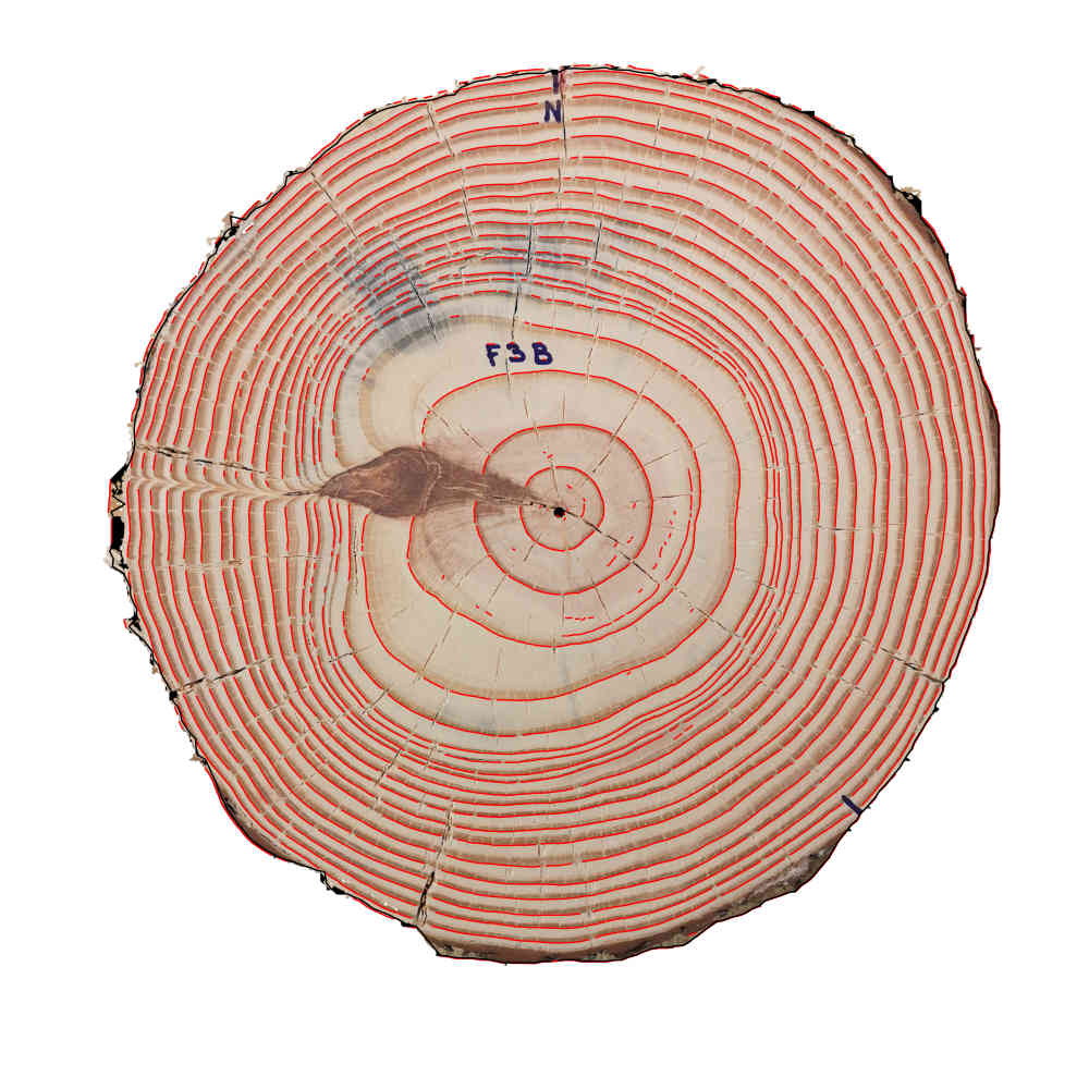
(e)

(f)

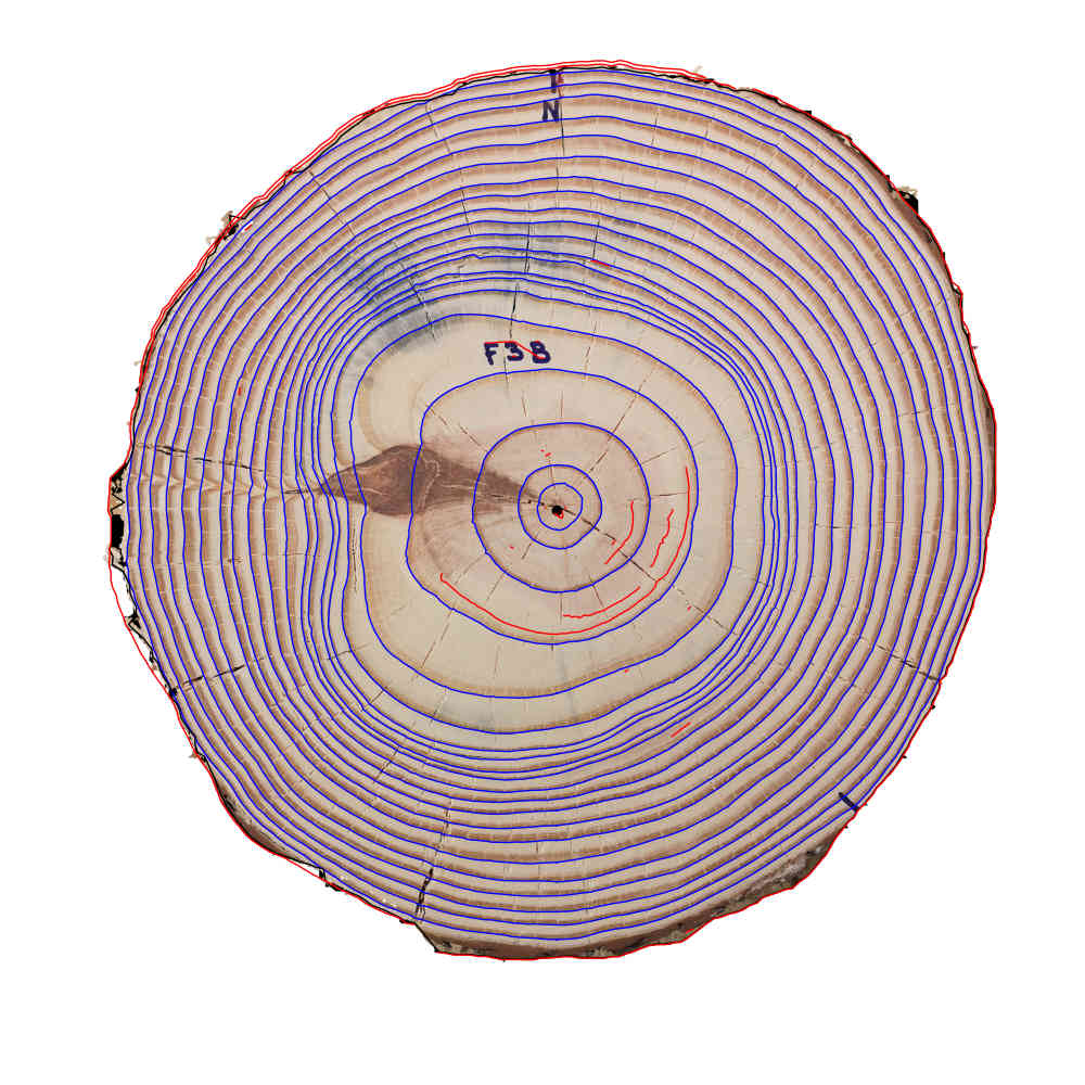
(g)

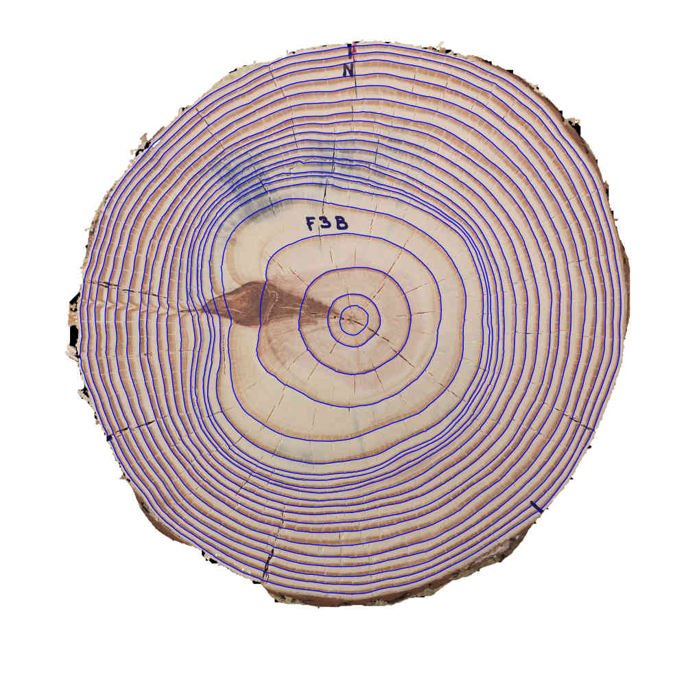
(h)

Figure 4: Principal steps of the CS-TRD tree-ring detection algorithm: (a) original image, (b) pre-processed image (resized, equalized, and converted to a grayscale image), (c) the output of the Canny Devernay edge detector, (d) edges filtered by the direction of the gradient, (e) set of detected chains, (f) connected chains, (g) post-processed chains and (h) detected tree-rings.

Input: $Im_{in}$, // segmented input image. Background pixels are in white (255)

$c$, // position of the pith in $Im_{in}$: center of the sypder web

$\sigma$, // Canny edge detector gaussian kernel parameter

$th_{low}$, // low threshold on the module of the gradient. Canny edge detector parameter

$th_{high}$, // high threshold on the module of the gradient. Canny edge detector parameter

$height$, // height of the image after the resize step

$width$, // width of the image after the resize step

$\alpha$, // threshold on the collinearity of the edge filtering, see Equation 3

$n_{r}$, // number of rays

$m_{c}$ // minimum chain length

Output: A list $l\_rings_{k}$, $k=1,2,\cdots,K$, where each element is a closed chain of points in the image, representing a tree-ring.

1 $im_{pre},c$ $\leftarrow$ preprocessing($Im_{in},height,width,c$) //see Algorithm 2

2 $m\_ch_{e},G_{x},G_{y}$ $\leftarrow$ canny_deverney_edge_detector($Im_{pre}$,$\sigma$,$th_{low}$,$th_{high}$) // described in [10]

3 $l\_ch_{f}$ $\leftarrow$ filter_edges($m\_ch_{e}$, $c$, $G_{x}$, $G_{y}$, $\alpha$, $Im_{pre}$) //see Algorithm 5

4 $l\_ch_{s},l\_nodes_{s}$ $\leftarrow$ sampling_edges($l\_ch_{f}$, $c$, $nr$, $m_{c}$, $Im_{pre}$) //see Algorithm 7

5 $l\_ch_{c},l\_nodes_{c}$ $\leftarrow$ connect_chains($l\_ch_{s}$,$l\_nodes_{s}$, $c$, $nr$) //see Algorithm 8

6 $l\_ch_{p}$ $\leftarrow$ postprocessing($l\_ch_{c}$,$l\_nodes_{c}$, $c$) //see Algorithm 19

7 $l\_rings$ $\leftarrow$ chain_to_labelme_json($l\_ch_{p}$, $height$, $width$, $c$, $Im_{in}$)// convert closed chains to json

return $l\_rings$

Algorithm 1 Tree-ring detection algorithm

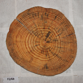
(a)

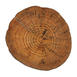
(b)

Figure 5: Background removal stage. Input (a) and output (b) using the code available from [21]

Given a segmented image of a tree slice -i.e., an image without a background- we need to find the set of pixel chains representing the annual rings (dark to clear transitions). We also need the center $c$ of the spider web (which corresponds to the tree’s pith) as input. Detecting this fundamental point is a problem that can be tackled by automatic means [4] or manually marked. In this article, we consider that this point is given (in the demo, both options are available).

Some algorithms have debug parameters. For example, in the function $connect\_chains$ of Algorithm 1, it is possible to set a debug flag to save all the intermediate results. To do that, we need the location where debugging results and the image at different stages will be saved (in some situations, debug results are saved by writing over the image). This paper does not discuss debug parameters because they are not crucial for the method understanding. The debug flag passes the debug parameters.

The first step in the Pipeline corresponds to preprocessing the input image to increase the method’s performance.

Preprocessing

The size of acquired images can vary widely, and this has an impact on the performance. On one side, the bigger the image, the slower the algorithm, as more data must be processed. On the other hand, if the image is too small, the relevant structures will be challenging to detect. Algorithm 2 shows the pseudo-code of the preprocessing stage. The first step is resizing the input image to a standard size of 1500x1500 pixels. In Section 6.2.1, we show a series of experiments that lead to choosing these dimensions. The size of the input image can vary, so zoom is applied in such a way as to zoom in or zoom out the input image so the image size for the rest of the processing is fixed. Pith coordinates must be resized as well. This step can be turned off by the user in the demo.

From lines 1 to 6, the former logic is implemented. The resize function (Line 5) is shown in Algorithm 3. The dimensions of the input image can vary, so image resize (Line 1, Algorithm 3) is applied using the function resize from Pillow library [2]. The method involves filtering to avoid aliasing if the flag image.ANTIALIAS is set. The center coordinates must be modified accordingly as well. To this aim, we use the following equations:

$$cy_{output}=cy*\frac{height_{output}}{height}\hskip 14.22636ptcx_{output}=cx*\frac{width_{output}}{width}$$ (1)

Where ($height$, $width$) is the input image dimensions, ($height_{output}$, $width_{output}$) is the output image dimension, and (cy, cx) is the (original resolution) disk pith location coordinates in pixels.

In line 7, the RGB image is converted to grayscale using the OpenCV [12] function:

$$cv2.cvtColor(img,cv2.COLOR\_BGR2GRAY)$$

Finally, in line 8, an histogram equalization step is applied to enhance contrast. The method is described in Algorithm 4. The first step (Line 1) changes the background pixels to the mean grayscale value to avoid undesirable background effects during equalization. Both equalized, and masked background images are returned. Then, in Line 2, the Contrast Limited Adaptive Histogram Equalization (CLAHE) [25] method for equalizing images is applied. We use the OpenCV implementation [12]. The threshold for contrast limiting is set to 10 by means of the $clipLimit$ parameter. Finally, in Line 3, the background of the equalized image is set to white (255).

Input: $Im_{in}$, // input image without background. Background pixel set to white (255)

Parameter:

$height_{output}$, // output image height, in pixels

$width_{output}$, // output image width, in pixels

$cy$, // pith’s coordinate y, in pixeles

$cx$, // pith’s coordinate x, in pixeles

Output: Preprocessed Image, pith coordinates scaled to the size of the preprocessed image

1 if None in [$height_{output}$, $width_{output}$ ] then

2       $Im_{r},cy_{output},cx_{output}$ $\leftarrow$ $(Im_{in},cy,cx)$

3 end if

4else

5       $Im_{r},cy_{output},cx_{output}$ $\leftarrow$ resize( $Im_{in},height_{output},width_{output},cy,cx$) // See Algorithm 3

6      

7 end if

8

9$Im_{g}$ $\leftarrow$ rgb2gray($Im_{r}$)

10 $Im_{pre}$ $\leftarrow$ equalize($Im_{g}$) // See Algorithm 4

return $[Im_{pre},cy_{output},cx_{output}]$

Algorithm 2 preprocessing

Input: $Im_{in}$, // the input image

Parameter:

$height_{output}$: // output image height, in pixels

$width_{output}$: // output image width, in pixels

$cy$: // pith’s coordinate y, in pixeles

$cx$: // pith’s coordinate x, in pixeles

Output: Resize image using Pillow Library

1 $Im_{r}$ $\leftarrow$ resize_image_using_pil_lib($Im_{in},height_{output},width_{output}$)

2$height,width$ $\leftarrow$ get_image_shape($Im_{in}$)

3 $cy_{output},cx_{output}$ $\leftarrow$ convert_center_coordinate_to_output_coordinate($cy,cx,height,width,height_{output},width_{output}$)// See Equation 1

return $[Im_{r},cy_{output},cx_{output}]$

Algorithm 3 resize

Input: $Im_{g}$, // gray scale input image. The background is white (255)

Output: Equalized image using OpenCV CLAHE [25] method

1 $Im_{pre},mask$ $\leftarrow$ change_background_intensity_to_mean($Im_{g}$)

2$Im_{pre}$ $\leftarrow$ equalize_image_using_clahe($Im_{pre}$)

3$Im_{pre}$ $\leftarrow$ change_background_to_value($Im_{pre},mask,255$)

return [$Im_{pre}$]

Algorithm 4 equalize

Canny-Devernay edge detector.

Line 2 of Algorithm 1, correspond to the edge detection stage. We apply the sub-pixel precision Canny Devernay edge detector [5, 10]. The output of this step is a list of pixel chains corresponding to the edges present in the image. Besides some noise-derived ones, we can group those edges into the following classes:

• $Edges_{T}$: edges produced by the tree growing process. It includes the edges that form the rings. Considering a direction from the pith outward, these edges are of two types: those produced by early wood to late wood transitions, expressed in the images as clear to dark transitions, and the latewood to early wood transitions, expressed as transitions from dark to clear in the images. We are interested in detecting the former ones, hereon called annual rings.

• $Edges_{R}$: mainly radial edges produced by cracks, fungi, or other phenomena.

• Other edges produced by wood knots.

The gradient vector is normal to the edge and encodes the local direction and sense of the transition. The Canny Devernay filter gives as output both the gradient of the image (composed by two matrices with the $x$ and $y$ components of the gradient, named $G_{x}$ and $G_{y}$) as well as the edge chains, in the form of a matrix, called $m\_ch_{e}$. Successive rows refer to chained pixels belonging to the same edge, and the row [-1,-1] marks the division between edges.

The Canny Devernay edge detector has the following parameters:

• $\sigma$: The standard deviation of the Gaussian kernel.

• $th_{low}$: Gradient threshold low, applied to the gradient modulus and associated with the two threshold hysteresis filtering on the edge points.

• $th_{high}$: Gradient threshold high, applied to the gradient modulus and associated to the two threshold hysteresis filtering on the edge points.

To use the Devernay-Canny implementation from [10], we needed to build a Python wrapper to execute that code. That code uses as input a PGM image. We feed the Devernay-Canny with the preprocessed image $Im_{pre}$ saved in disk with that format.

Regarding the output, $m\_ch_{e}$ is a matrix, where each row refers to the pairs $(x,y)$, the coordinates of the edges. Each Devernay curve in the list is separated from the next one by a $(-1,-1)$. Minor code modifications were needed in the IPOL implementation of the Canny Devernay filter [10] to get the image gradient matrices $G_{x}$ and $G_{y}$ as output.

Filtering the edge chains

We filter out all the points of the edge chains for which the angle between the gradient vector and the direction of the ray touching that point are greater than $\alpha$ (30 degrees in our experiments). The $Edges_{T}$ produced by the early wood transitions points inward, and the $Edges_{R}$, for which the normal vector is roughly normal to the rays, are filtered out. Note that this process breaks an edge chain into several fragments. This is done by Algorithm 5.

Given the center $c$ and a point $p_{i}$ over an edge curve, the angle $\delta(\vec{cp_{i}},\vec{G_{p_{i}}})$ between the vector $\vec{cp_{i}}$ at the point $p_{i}$ and the gradient vector $\vec{G_{p_{i}}}$ (Figure 6) at the same point is given by:

$$\delta(\vec{cp_{i}},\vec{G_{p_{i}}})=\arccos\left(\frac{\vec{cp_{i}}\times\vec{G_{p_{i}}}}{\|\vec{cp_{i}}\|\|\vec{G_{p_{i}}}\|}\right)$$ (2)

We filter out all the points $p_{i}$ for which the angle $\delta(\vec{cp_{i}},\vec{G_{p_{i}}})$ is greater than the parameter $\alpha$:

$$\delta(\vec{cp_{i}},\vec{G_{p_{i}}})\geq\alpha$$ (3)

The filter edges method is shown at Algorithm 5. It gets as input the Deverney edges $m\_ch_{e}$, the pith center, the image gradient components in the form of two matrices $G_{x}$ and $G_{y}$ and the preprocessed image $Im_{pre}$. It needs the $\alpha$ threshold of Equation 3 as a parameter. From lines 1 to 5, it computes the angle between vector $\vec{cp_{i}}$ and the gradient $\vec{G_{p_{i}}}$ at point $p_{i}$. We use the Python numpy library matrix operations to speed up computation. In line 1, we change the edge reference axis. Figure 6 shows vectors $\vec{Op_{i}}$ and $\vec{cp_{i}}$, as well as the gradient $\vec{G_{p_{i}}}$ at edge point $p_{i}$. The function change_reference_axis change the vector coordinate reference from $\vec{Op_{i}}$ to $\vec{cp_{i}}$ and produces a new matrix $Xb$. This is made by subtracting the pith vector from each row. Matrix $Xb$ still has the delimiting edges curve rows with the value [-1,-1]

Each edge gradient is saved in matrix $G$ (line 2), keeping the same edge order of the matrix $m\_ch_{e}$; this means that

$$p_{i}=m\_ch_{e}[i]\rightarrow\vec{G_{p_{i}}}=G[i]$$

Where $p_{i}$ is the i-row of matrix $m\_ch_{e}$ and $\vec{G_{p_{i}}}$ is the i-row of matrix $G[i]$.

In Lines 3 and 4, the matrices $Xb.T$($Xb$ transposed matrix) and $G$ are normalized, dividing the vector by the norm as shown in Equation 4, simplifying Equation 2:

$$\delta(R_{i},\vec{G_{p_{i}}})=\arccos\left(\frac{\vec{cp_{i}}\times\vec{G_{p_{i}}}}{\|\vec{cp_{i}}\|\|\vec{G_{p_{i}}}\|}\right)=\arccos\left(\frac{\vec{cp_{i}}}{\|\vec{cp_{i}}\|}\times\frac{\vec{G_{p_{i}}}}{\|\vec{G_{p_{i}}}\|}\right)=\arccos\left(\vec{cp_{i}}_{unit}\times\vec{G_{p_{i}}}_{unit}\right)$$ (4)

In line 5, Equation 4 is computed in matrix form, and the angle between normalized vectors $\vec{G_{p_{i}}}_{unit}$ and $\vec{cp_{i}}_{unit}$ is returned in degrees in the matrix $\theta$. In line 6, the edge filtering is applied, following  Equation 3. If the edge point $p_{i}$ is filtered out, then $X_{edges\_filtered}[i]=[-1,-1]$. The edges are converted to curve objects in line 7. We say that two edge pixels belong to the same edge if, between them, it does not exist a row in matrix $X_{edges\_filtered}$ with values [-1,-1]. The object Curve inherits the properties of the class LineString from the shapely package, which is used in the sampling edges stage.

Finally, in lines 8 and 9, the curve belonging to the border edges is computed and added to the curve list, $l\_ch_{f}$. In this context, we name $border$, the limits of the segmented image concerning the background. The function $get\_border\_curve$ is shown in Algorithm 6. We use a simple method to compute the border edges. First, we generate a mask which is an image of the same dimensions as $Im_{pre}$, enlarged by $3$ lines and $3$ columns before the first and after the last line and columns to avoid border effects of the filtering. The mask image has two values, $0$ for the region of the wood slice and $255$ for the background. Lines 1 to 4 calculate the mask image. In line 1 we threshold $Im_{pre}$ masking all the pixels with a value equal to 255, particularly the background. Some internal pixels can also have a value equal to 255. To avoid those pixels in the mask, we blur the mask (line 2), using a Gaussian Kernel with a high $\sigma$ (in our implementation $\sigma=11$), and we set to 255 all the pixels with a value higher than 0 (lines 2 and 3). In line 4, the mask is padded with $pad=3$. Finally, in line 5, we apply an OpenCV finding contour method to get the border contour on the mask. The OpenCV implementation returns all the contours it finds, including the image’s border. We select the contour for which the enclosed area is closest to half the image. This is a criterion that works fine for this purpose. In line 6, the contour object is converted to a Curve object.

Input: $m\_ch_{e}$, // matrix of edge curves

$c$, // center of the spider web, in pixels: $c_{x}$ and $c_{y}$

$G_{x}$, // X component of the gradient, a matrix

$G_{y}$, // Y component of the gradient, a matrix

$Im_{pre}$, // Preprocessed image

Parameter:

$\alpha$, //Threshold edge filter, Equation 3

Output: A list $l\_ch^{k}_{f}$, $k=1,2,\cdots,N$, where each element is a filtered edge curve

1 $Xb$ $\leftarrow$ change_reference_axis($m\_ch_{e}$, $c_{y}$, $c_{x}$)

2 $G$ $\leftarrow$ get_gradient_vector_for_each_edge_pixel($l\_ch_{e}$, $G_{x}$, $G_{y}$)

3 $Xb_{normalized}$ $\leftarrow$ normalized_row_matrix(Xb.T)

4 $G_{normalized}$ $\leftarrow$ normalized_row_matrix(G)

5 $\theta$ $\leftarrow$ compute_angle_between_gradient_and_edges($Xb_{normalized}$, $G_{normalized}$)

6 $X_{edges\_filtered}$ $\leftarrow$ filter_edges_by_threshold($m\_ch_{e}$, $\theta$, $\alpha$)

7 $l\_ch_{f}$ $\leftarrow$ convert_masked_pixels_to_curves($X_{edges\_filtered}$)

8 $border\_curve$ $\leftarrow$ get_border_curve($Im_{pre}$, $l\_ch_{f}$)// See Algorithm 6

9 $l\_ch_{f}$ $\leftarrow$ $l\_ch_{f}$ + $border\_curve$

return $l\_ch_{f}$

Algorithm 5 filter_edges

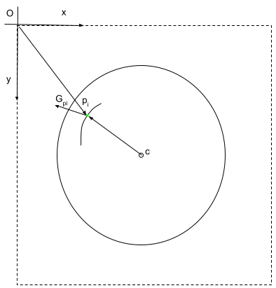
Figure 6: Coordinates reference of edge $p_{i}$, vector $\vec{Op_{i}}$. Edge filtering computation use vector $\vec{cp_{i}}$. $O$ represents the origin of the image coordinate axis. $C$ represents the pith position

Input: $Im_{pre}$, // Preprocessed image

$l\_ch_{f}$, //list of object Curves

Output: $border\_curve$

1 $mask$ $\leftarrow$ mask_background($Im_{pre}$)

2 $mask$ $\leftarrow$ blur($mask$)

3 $mask$ $\leftarrow$ thresholding($mask$)

4 $mask$ $\leftarrow$ padding_mask($mask$)

5 $border\_contour$ $\leftarrow$ find_border_contour($mask$, $Im_{pre}$)

6 $border\_curve$ $\leftarrow$ contour_to_curve($border\_contour$, len($l\_ch_{f}$))

return $border\_curve$

Algorithm 6 get_border_curve

Sampling edges

Given the set of filtered chained edge points $l\_ch_{f}$, a list of curves, we sample each curve using the number of rays $Nr$. The Algorithm 7 describe the procedure. Two parameters are included in this algorithm: $Nr$, the number of rays (360 by default), and $min\_chain\_lenght$, the minimum number of nodes in a chain (the object chain is described in the following paragraph). Every chain has two endpoints, so we fix $min\_chain\_lenght=2$.

This algorithm produces as output two lists: one of the objects Chain named $l\_ch_{s}$ and one of the objects Nodes named $l\_nodes_{s}$, which includes all the nodes in all the chains. The object Chain contains a list of pointers to all the nodes belonging to that chain ($l\_nodes$). This allows us to find all the nodes of a given chain. The object Node contains the identifier of the chain to which it belongs ($chain\_id$). There is no chain without nodes, nor nodes belonging to more than one chain.

An object Chain has the following attributes:

• $l\_nodes$: chained list of the nodes belonging to the chain.

• $id$: identification of the chain.

• $Nr$: total number of rays on the disk.

• $extA$: first endpoint of the chain, named node A.

• $extB$: second endpoint of the chain, named node B.

• $type$: We define three chain types: border, normal, and center.

• $B\_outward$: Pointer to the next chain above the B node.

• $B\_inward$: Pointer to the next chain below the B node.

• $A\_outward$: Pointer to the next chain above the A node.

• $A\_inward$: Pointer to the next chain below the A node.

We use the concepts of outward and inward in the attributes of a chain. Both are related to a given endpoint (A or B). Given a chain endpoint and the corresponding ray, we find the first chain that intersects that ray going from the chain to the center (named here as inward) and the first chain that intersects that ray going from the chain moving away from the center (named here as outward). Figure 8 illustrate this. Chains are superposed over the gray-level image. The ray at endpoint A is in blue, the nodes are in red at the intersection between the rays, and the chains are in orange, black, and yellow. Orange and yellow chains are the visible chains for the black chain at endpoint A (outward and inward, respectively); this concept is explained later. Every chain has two endpoint nodes, A and B. Endpoint A is always the furthest node clockwise, while endpoint B is the most distant node counterclockwise.

An Object Node has the following attributes:

• $(x,y)$ node coordinates. Floating point numbers.

• $chain\_id$: identification of the chain to which the node belongs.

• $radial\_distance$: Euclidean distance to the center. It is a floating point number.

• $angle$: angle orientation of the ray passing by that node, in degrees. It is a floating point number.

Three metric distances between chains are defined. Given a chain endpoint $EndPoint_{j}$(the selected endpoint for the current chain $Ch_{j}$) and $EndPoint_{k}$ (the selected endpoint for chain $Ch_{k}$) distances are defined as:

• Euclidean Given endpoint cartesian coordinates ($x$,$y$), the distance between endpoints is defined as

  $$\sqrt{\left(x_{j}-x_{k}\right)^{2}+\left(y_{j}-y_{k}\right)^{2}}$$ (5)

  Where $(x_{j},y_{j})$ are the cartesian coordinates of $Endpoint_{j}$ and $(x_{k},y_{k})$ are the cartesian coordinates of $Endpoint_{k}$.

• Radial Difference Given the endpoint Euclidean distance to the pith center, this distance is defined as

  $$\|r_{j}-r_{k}\|$$ (6)

  Where $r_{j}$ is the Euclidean distance of $Endpoint_{j}$ to the pith center, and $r_{k}$ is the Euclidean distance of $Endpoint_{k}$ to the pith center.

• Angular Given the endpoints ray support angle, $\theta$ (radii angular direction) this distance is defined as

  $$\left(\theta_{j}-\theta_{k}+360\right)mod\hskip 5.69046pt360$$ (7)

  Where $\theta_{j}$ is the direction of the ray supporting $Endpoint_{j}$ (in degrees), $\theta_{k}$ is the direction of the ray supporting $Endpoint_{k}$ (in degrees), and $mod$ refers to the module operation. Figure 7 illustrates angle $\theta_{j}$ of $Ray_{j}$ given the disk pith position $C$.

Figure 7: Ray references axis. $C$ is the pith center. $\theta_{j}$ is the angle of $Ray_{j}$

.

Algorithm 7 extract the image dimensions from the preprocessed image $Im_{pre}$. Then we proceed to build the rays. A ray object is a semi-line, with one endpoint at the center $c$ (the pith) and the other at the image border. This gives a list of $Nr$ rays. Then, we compute the intersections between curves and rays using the Shapely python library. Note that a curve produced by Devernay is a set of chained pixels, and some of them are also nodes, as shown in Figure 3(c). Once the Nodes are found, we create a chain including only the nodes and not all the points of the corresponding Devernay curve. In this sense, a chain is a sampled curve. If a chain has less than $min\_chain\_lenght$ nodes, we delete it. Finally, we build two artificial chains. One of type center. This artificial chain has $Nr$ nodes, all with the same $(x,y)$ coordinates but different angular orientations. The second one is the disk border. Both artificial chains are beneficial at the connecting chain stage. The field $type$ in the Chain object identifies if the chain is a normal one or is one of the two artificial chains just described.

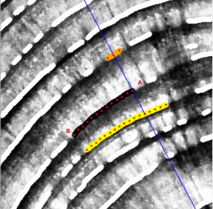
Figure 8: A given chain (in black) with two endpoints A and B. Its nodes (in red) appear at the intersection between the Canny Devernay curve and the rays. The ray at endpoint A is in blue. Other chains detected by Canny Devernay are colored in white. Endpoint A’s inward and outward chains are in yellow and orange, respectively.

Input: $l\_ch_{f}$, // list of curves

$c$, // center of the sypder web

$Im_{pre}$ // preprocessed image

Parameters:

$min\_chain\_lenght$, // minimum length of a chain

$nr$ // number of total rays

Output: A list $l\_ch^{k}_{s}$, $k=1,2,\cdots,N$, where each element is a chain;

$l\_nodes^{k}_{s}$, $k=1,2,\cdots,N_{n}$, where each element is a Node

1 $height$, $width$ $\leftarrow$ $Im_{pre}$.shape

2 $l\_rays$ $\leftarrow$ build_rays($nr$, $height$, $width$, $c$)

3 $l\_ch_{s}$,$l\_nodes_{s}$ $\leftarrow$ intersections_between_rays_and_devernay_curves($c$, $l\_rays$ , $l\_ch_{f}$, $min\_chain\_lenght$, $nr$, $height$, $width$)

4 $l\_ch_{s}$,$l\_nodes_{s}$ $\leftarrow$ generate_virtual_center_chain(c, nr, $l\_nodes_{s}$, $l\_ch_{s}$)

return $l\_ch_{s}$,$l\_nodes_{s}$

Algorithm 7 sampling_edges

Connect chains

We must now group this set of chains to form the rings. Some of these chains are spurious, produced by noise, small cracks, knots, etc., but most are part of the desired rings, as seen in Figure 4.

To connect chains, we must decide if the endpoints of two given chains can be connected, as illustrated by Figure 9. We use a support chain, $Ch_{0}$ in the figure, to decide whether or not those chains must be connected.

(a)

(b)

Figure 9: An illustration of the connectivity issue. (a) The question is if endpoint A of $Ch_{3}$ must be connected to endpoint B of $Ch_{2}$ (red dashed line) or to endpoint B of $Ch_{1}$ (blue dashed line). In figure (b), the same question can be posed for the connection between endpoint B of $Ch_{1}$ and endpoint A of $Ch_{2}$, but $Ch_{1}$ and $Ch_{2}$ intersect (the endpoints are crossed by the same ray), and so this connection is forbidden. Note that we represent the connections by line segments for clarity, but in fact, these are curves in the image space, as we interpolate between chain endpoints in polar geometry

Figure 10: For the chain support $Ch_{0}$, the set of chain candidates is formed by $Ch_{1}$, $Ch_{2}$, $Ch_{4}$, $Ch_{5}$ and $Ch_{6}$. Chain $Ch_{3}$ is shadowed by $Ch_{1}$ but $Ch_{5}$ is not shadowed by $Ch_{6}$ because at least one endpoint of $Ch_{5}$ is visible from $Ch_{0}$. Note that a chain becomes part of the candidate chains set if at least one of its endpoints is visible from the chain support.

.

To group chains that belong to the same ring, we proceed as follows:

1. We order all the chains by length and begin processing the longest. The processed chain is called Chain support, $Ch_{i}$. Once we finish merging all the possible candidate chains related to that one ($candidates_{Ch_{i}}$), we do the same with the next longest chain.

2. We find the chains that are visible from the Chain support inwards (i.e., in the direction from Chain support to the center). The concept of visibility here means that at least one endpoint of the candidate chain is visible from the Chain support. Visible means that a ray that goes through the endpoint of the candidate chain crosses the chain support without crossing any other chains in between. The set of candidate chains of the Chain support $Ch_{i}$ is named $candidates_{Ch_{i}}$. This is illustrated by Figure 10, in which case, the chains candidates generated inwards by $Ch_{0}$ is:

   $$candidates_{Ch_{0}}=\{Ch_{1},Ch_{2},Ch_{4},Ch_{5},Ch_{6}\}$$

   Chain $Ch_{3}$ is shadowed by $Ch_{1}$ and $Ch_{5}$ is not shadowed by $Ch_{6}$ because at least one of its endpoints are visible from $Ch_{0}$. The same process is made for the chains visible from the Chain support outwards.

3. We go through the set $candidates_{Ch_{i}}$ searching for connections between them. By construction, the chain support is not a candidate to be merged in this step. From the endpoint of a chain, we move forward angularly. The next endpoint of a nonintersecting chain in the $candidates_{Ch_{i}}$ set is a candidate to be connected to the first one. We say that two chains intersect if there exists at least one ray that cross both chains. For example, in Figure 10, $Ch_{6}$ intersects with $Ch_{5}$ and non-intersects with $Ch_{4}$. To decide if both chains must be connected, we must measure the connectivity goodness between them.

4. To define a notion of connectivity goodness, we combine three criteria:

   1. Radial tolerance for connecting chains. The radial difference between the distance from each chain to be merged (measured at the endpoint to be connected) and the support chain must be small. For example, in Figure 11, if we want to connect node $N_{i}$ of $Ch_{l}$ and node $N_{i+1}$ of $Ch_{k}$, we must verify that

      $$\delta R_{i}*(1-Th_{Radial\_tolerance})\leq\delta R_{i+1}\leq\delta R_{i}*(1+Th_{Radial\_tolerance})$$

      Where $Th_{Radial\_tolerance}$ is a parameter of the algorithm. We call this condition RadialTol.

      Figure 11: Quantities used to measure the connectivity between chains. $\delta R_{i}$ is the radial difference between two successive chains along a ray $R_{i}$ and $\delta N_{i}$ is the radial difference between two successive nodes $N_{i}$ and $N_{i+1}$. Note that these nodes can be part of the same chain or be part of two different chains that may be merged. Support chains are represented with the name $Ch_{i}$. $Ch_{i}$ visible chains are $Ch_{j}$, $Ch_{l}$ and $Ch_{k}$. Chains $Ch_{j}$ and $Ch_{k}$ satisfy similarity conditions

      .

   2. Similar radial distances of nodes in both chains. For each chain, we define a set of nodes. For the chain $Ch_{j}$, this set is $N_{j}=\{N_{j}^{0},N_{j}^{1},...,N_{j}^{n_{nodes}}\}$ where $n_{nodes}$ is the number of nodes to be considered, a parameter. See Figure 12. We use the whole chain if it is shorter than $n_{nodes}$. We measure $\delta R_{i}$, the radial distance between a node in the given chain and the corresponding node for the same ray in the support chain, as illustrated in Figure 11. This defines two sets, one for each considered chain $i$ and $k$: $Set_{j}=\{\delta R_{j}^{0},..,\delta R_{j}^{n_{nodes}}\}$ and $Set_{k}=\{\delta R_{k}^{0},..,\delta R_{k}^{n_{nodes}}\}$. We calculate the mean and the standard deviation $Set_{j}(\mu_{j},\sigma_{j})$ and $Set_{k}(\mu_{k},\sigma_{k})$. The size of the distribution is defined by the parameter $Th_{Distribution\_size}$. This defines a range of radial distances associated with each chain: $Range_{j}=(\mu_{j}-\textit{$Th_{Distribution\_size}$}*\sigma_{j},\mu_{j}+\textit{$Th_{Distribution\_size}$}*\sigma_{j})$ and $Range_{k}=(\mu_{k}-\textit{$Th_{Distribution\_size}$}*\sigma_{k},\mu_{k}+\textit{$Th_{Distribution\_size}$}*\sigma_{k})$. To connect both chains, there must be a non-null intersection between both distributions: $Range_{j}\cap Range_{k}\neq 0$. We call this condition SimilarRadialDist.

   3. Regularity of the derivative. Suppose we have two chains $Ch_{j}$ and $Ch_{k}$ that can be connected and a set of interpolated nodes between the endpoints of those chains (let’s call $Ch_{jk}$ the set of interpolated nodes between $Ch_{j}$ and $Ch_{k}$, indicating that they form a new ”interpolating” chain). See Figure 12. The new virtual chain created by the connection between chains $Ch_{j}$ and $Ch_{k}$ will encompass the nodes of those two chains and the new interpolated nodes between both chains ($Ch_{jk}$, colored in red in the figure). To test the regularity of the derivative, we define a set of nodes for each concerned chain. For the chain $Ch_{j}$, this set is $\{N_{j}^{0},N_{j}^{1},...,N_{j}^{n_{nodes}}\}$ where $n_{nodes}$ is the number of nodes to be considered, a parameter ($n_{nodes}=20$ in the current implementation). We use all its nodes if the chain is shorter than $n_{nodes}$. For each chain, we compute the centered derivative in each node, $\delta N^{s}=\frac{\|r_{s+1}-r_{s-1}\|}{2}$, where $r_{s}$ is the radial distance of the node $N^{s}$ to the center (i.e., the Euclidean distance between the node and the center of the spider web). Therefor radial distance to center of node $N^{s-1}$ is represented as $r_{s-1}$ and radial distance to center of node $N^{s+1}$ is represented as $r_{s+1}$. The set of derivatives for the nodes of the existing chains is $Der(Ch_{j},Ch_{k})=\{\delta N_{j}^{0},...,\delta N_{j}^{n_{nodes}},\delta N_{k}^{0},...,\delta N_{k}^{n_{nodes}}\}$. The condition $Th_{regular\_derivative}$ is asserted if the maximum of the derivatives in the interpolated chain is less or equal to the maximum of the derivatives in the two neighboring chains times a given tolerance:

      $$max(Der(Ch_{jk}))\leq max(Der(Ch_{j},Ch_{k}))\times Th_{Regular\_derivative}$$

      Where $Th_{Regular\_derivative}$ is a parameter. We call this condition RegularDeriv.

   Figure 12: Nomenclature used for the connect chains algorithm. Given the support chain, $Ch_{i}$, chains $Ch_{j}$ and $Ch_{k}$ are candidates to be connected. $N_{j}^{n}$ are the nodes of $Ch_{j}$, with $n=0$ for the node corresponding to the endpoint to be connected. Similarly, we note $N_{k}^{n}$ the nodes of $Ch_{k}$. In red are the nodes created by an interpolation process between both endpoints. We represent the radial distance to the center of $Node^{s}$ as $r_{s}$.

   In order to connect chains $Ch_{j}$ and $Ch_{k}$, the following condition must be met:

   $$\textit{RegularDeriv}\land(\textit{SimilarRadialDist}\lor\textit{RadialTol})$$ (8)

   where $\lor$ and $\land$ stands for the logical or and and symbols, respectively.

   Another condition must be met: no other chain must exist between both chains to be connected. If another chain exists in between, it must be connected to the closer one. For example, in Figure 10, it is impossible to connect chains $Ch_{3}$ and $Ch_{5}$ because between them appear $Ch_{4}$. We call this condition ExistChainOverlapping. Consequently, Equation 8 is modified as follows

   $$\mathbf{not}\textit{ExistChainOverlapping}\land\textit{RegularDeriv}\land(\textit{SimilarRadialDist}\lor\textit{RadialTol})$$ (9)

   The symbol $\mathbf{not}$ stands for the not operator.

   The method iterates this search for connectivity between chains over different neighborhood sizes. The parameter NeighbourdhoodSize defines the maximum allowed distance, measured in degrees, for connecting two chains. If the distance between two chains endpoints is longer than NeighbourdhoodSize, those chains are not connected.

   The parameter derivFromCenter controls how are estimated the interpolated nodes between two chains, as the ones in red in Figure 12. If $derivFromCenter=1$, ray angle and radial distance from the center are used to estimate the position of the interpolated nodes. If it is set to 0, the estimation is made by measuring the radial distance to the support chain.

   We iterate this process for the whole image for five sets of parameters: $Th_{Radial\_tolerance}$, $Th_{Distribution\_size}$, $Th_{Regular\_derivative}$, NeighbourdhoodSize and derivFromCenter. In each iteration, we relax the parameters. In the first iteration, there are a lot of small chains, but in the second and third iterations, the concerned chains are already more extended and less noisy. Once the merging process is advanced, we can relax the parameters to connect more robust chains. Table 1 summarize the parameter sets.

   	1	2	3	4	5	6	7	8	9
   $Th_{Radial\_tolerance}$	0.1	0.2	0.1	0.2	0.1	0.2	0.1	0.2	0.2
   $Th_{Distribution\_size}$	2	2	3	3	3	3	2	3	3
   $Th_{Regular\_derivative}$	1.5	1.5	1.5	1.5	1.5	1.5	2	2	2
   NeighbourdhoodSize	10	10	22	22	45	45	22	45	45
   derivFromCenter	0	0	0	0	0	0	1	1	1

   Table 1: Connectivity Parameters. Each column is the parameter set used on that iteration.

5. We proceed in the same manner in the outward direction.

The former ideas are implemented in Algorithms 8 and 9. Algorithm 8 defines the logic for iterating over the constraints defined in Table 1. In line 1, a square binary intersection matrix $M$ is computed. Precompute matrix $M$ will speed up the procedure. Rows and columns of $M$ span the chain list. Chain $Ch_{j}$ intersect chain $Ch_{k}$ if $M[j,k]=1$. We say that two chains intersect if at least one ray crosses both chains. Lines 2 to 6 are iterated for each parameter set of Table 1. Line 3 defines the parameters for each iteration. The dictionary $iteration\_params$ has keys for the nodes and chains lists. Both lists may be updated at each iteration because chains may be connected. When two chains are connected, $M$ is updated as well. In the final iteration ($i=9$), the external border chain is added to the chain list in order to be used as a support chain. In line 4, the function which connects the chains is called, returning the updated nodes and chains lists and $M$ after the connecting stage. Finally, in line 5, nodes and chains lists are updated in the $iteration\_params$ dictionary for the next iteration.

Input: $l\_ch_{s}$,// chains list

$l\_nodes_{s}$,// nodes list

$c$, // center of the spider web

$nr$// number of total rays

Output: A list $l\_ch^{f}_{c}$, $f=1,2,\cdots,N_{f}$, where each element is a chain;

$l\_nodes^{f}_{c}$, $c=1,2,\cdots,N_{f}$, where each element is a Node

1 $M$ $\leftarrow$ compute_intersection_matrix($l\_ch_{s}$, $l\_nodes_{s}$, $nr$).

/* Loop for connecting chain main logic, losing the restrictions at each iteration */

2 for $i\leftarrow 1$ to $9$ do

3       $iteration\_params$ $\leftarrow$ get_iteration_parameters($i$)//Table (1)

4       $l\_ch_{c}$, $l\_nodes_{c}$, $M$ $\leftarrow$ connect_chain_main_logic($M$, $c$, $nr$, $iteration\_params$) //see Algorithm 9

5       update_list_for_next_iteration($l\_ch_{c},l\_nodes_{c}$)

6 end for

return $l\_ch_{c}$,$l\_nodes_{c}$

Algorithm 8 Connect Chains

Algorithm 9 shows the connectivity main logic. State class manages the support chain iteration logic. It contains references to the lists of all the chains and nodes and stores the similarity parameters and the intersection matrix, $M$. Essentially, the State class is the hub of our system, containing all the necessary information to operate. The system comprises all the chains and nodes, and the M intersection matrix.

The State class updates the chains and nodes lists and the matrix $M$ whenever two chains are connected. This update is critical for our operation and signifies that the system has been modified.

Lines 1 and 2 are initializations. Initialization consists of:

1. Sort the chain list by size (i.e. number of nodes) in descending order.

2. To optimize our method for searching visible chains from the chain support, we assign pointers to the visible inward and outward chains at both endpoints (A and B) of each chain.

The loop between lines 4 and 20 is applied to all the chains as long as $State_{i}\neq State_{i-1}$. The condition $State_{i}=State_{i-1}$ is true when no connections are made after an iteration. In line 4, we get a new support chain, $Ch_{i}$, for the current iteration. The logic to get the next chains are grouped in the methods $get\_next\_chain$ (line 4) and $update\_system\_state$ (line 20), described inAlgorithm 11 and Algorithm 10 respectively. Support chains are iterated following a neighborhood logic for speeding up purposes instead of iterating over the list sequentially.

In line 5, outward and inward visible chains are obtained and stored in $l\_s\_outward$ and $l\_s\_inward$ lists. To this aim we iterate over $l\_ch_{s}$ and check if visibility chain pointers ($B\_outward$, $B\_inward$, $A\_outward$, $A\_inward$) refers to $Ch_{i}$. The loop between lines 7 and 19 explores the lists $l\_s\_inward$ and $l\_s\_outward$ with iteration variable $l\_candidates\_Chi$. First, the $j\_pointer$ index is set to 0. Then, from lines 8 to 11, we set the variable $location$ to signal if $l\_candidate_{Ch_{i}}$ is the inward or the outward list. We iterate over the set $l\_candidates\_Chi$ to look for similar chains, using the similarity criterion defined in Equation 9. The loop over the chains in the subset $l\_candidates\_Chi$ goes from line 12 to 19. The current chain, $Ch_{j}$, inside the inner while loop, is indexed by the $j\_pointer$ index. In line 14, all chains in the subset $l\_candidates\_Chi$ not intersecting with chain $Ch_{j}$ are chosen. As rings do not intersect each other, candidates to be part of the same ring can not intersect between them. Line 15 detects $Ch_{k}^{b}$, the closest chain in $l\_candidates\_Chi$ to endpoint B of $Ch_{j}$, that satisfies the similarity constraints (Algorithm 16), and line 16 does the same for $Ch_{k}^{a}$ concerning endpoint A of $Ch_{j}$. Line 17 selects which is closest to its corresponding endpoint in $Ch_{j}$. Line 18 calls the function that connects the closest one to the corresponding endpoint using the Euclidean distance between them (Algorithm 14); finally, in line 19, $j\_pointer$ is updated. If two chains are connected over this iteration, then in the next iteration, we iterate again over $Ch_{j}$. Note that when two chains are connected, the candidate chain ($Ch_{k}$) is deleted from the list of candidate chains, and their nodes are added to chain $Ch_{j}$. In line 20, we update the outer while loop system variables to define if the process is finished (i.e., all chains are connected). In line 21, we iterate over all the chains in list $l\_Ch_{s}$, and if the chain has enough nodes, we complete it, following Algorithm 12. Finally, we return the connected chain list and their nodes, $l\_ch_{c}$ and $l\_nodes_{c}$, respectively.

Input: $M$ //Binary Matrix with intersection chains info

$c$, // center of the sypder web

$nr$, // number of total rays

Parameters:

$l\_ch_{s}$, // chains list

$l\_nodes_{s}$, // nodes list

$th\_radial\_tolerance$, // Radial tolerance for connecting chains

$th\_distribution\_size$, // Chains Radial Difference Standard deviations for connecting chains

$th\_regular\_derivative$, // Chains Radial Derivative threshold for connecting chains

$neighbourhood\_size$, //Max Angular distance allowed for connecting chains

$derivative\_from\_center$ // Related to how nodes are interpolated

Output: A list $l\_ch^{k}_{c}$, $k=1,2,\cdots,N_{f}$, where each element is a chain,

$l\_nodes^{k}_{c}$, $k=1,2,\cdots,N_{f}$, where each element is a Node

1 $State_{i-1}$ $\leftarrow$ 0

2 $State_{i}$ $\leftarrow$ init_system($l\_ch_{s}$, $l\_nodes_{s}$, $M$ , $c$, $nr$,$th\_radial\_tolerance$, $th\_distribution\_size$, $th\_regular\_derivative$, $neighbourhood\_size$, $derivative\_from\_center$)

3 while $State_{i}\neq State_{i-1}$ do

4       $Ch_{i}$ $\leftarrow$ get_next_chain($State_{i}$)//See Algorithm 11

5       $l\_s\_outward$, $l\_s\_inward$ $\leftarrow$ get_chains_in_and_out_wards($l\_ch_{s}$,$Ch_{i}$)

6       for $l\_candidates\_{Ch_{i}}$ in ($l\_s\_outward$, $l\_s\_inward$) do

7             $j\_pointer$ $\leftarrow$ 0

8             if $l\_candidates\_{Ch_{i}}$ == $l\_s\_inward$ then

9                   $location$ $\leftarrow$ ”inward”

10            else

11                   $location$ $\leftarrow$ ”outward”

12            

13            while length($l\_candidates\_{Ch_{i}}$) $>$ $j\_pointer$ do

14                   $Ch_{j}$ $\leftarrow$ $l\_candidates\_{Ch_{i}}$[$j\_pointer$]

15                   $l\_no\_intersection\_j$ $\leftarrow$ get_non_intersection_chains($M$, $l\_candidates\_{Ch_{i}}$, $Ch_{j}$)

16                   $Ch_{k}^{b}$ $\leftarrow$ get_closest_chain_logic($State_{i}$, $l\_candidates\_{Ch_{i}}$, $Ch_{j},l\_no\_intersection\_j,Ch_{i},location$, $B$)//See Algorithm 15

17                   $Ch_{k}^{a}$ $\leftarrow$ get_closest_chain_logic($State_{i}$, $l\_candidates\_{Ch_{i}}$, $Ch_{j},l\_no\_intersection\_j,Ch_{i},location$, $A$)//See Algorithm 15

18                   $Ch_{k}$, $endpoint$ $\leftarrow$ select_closest_one($Ch_{j}$, $Ch_{k}^{a}$, $Ch_{k}^{b}$)

19                   connect_two_chains($State_{i}$, $Ch_{j}$, $Ch_{k}$, $l\_candidates\_{Ch_{i}}$, $endpoint$, $Ch_{i}$)//See Algorithm 14

20                   $j\_pointer$ $\leftarrow$ update_pointer($Ch_{j}$, $Ch_{k}$, $l\_candidates\_{Ch_{i}}$)

21                  

22            

23      $State_{i}$, $State_{i-1}$ $\leftarrow$ update_system_status( $State_{i}$, $Ch_{i}$, $l\_s\_outward$, $l\_s\_inward$)//See Algorithm 10

24      

25$l\_ch_{c}$,$l\_nodes_{c}$ $\leftarrow$ iterate_over_chains_list_and_complete_them_if_met_conditions($State_{i}$)

26

return $l\_ch_{c}$,$l\_nodes_{c}$

Algorithm 9 Connect Chains Main Logic

Methods $get\_next\_chain$ and $update\_system\_state$ contain the logic to get $Ch_{i}$ at the current iteration. The former is the primary one and is described in Algorithm 10 (a method of $State_{i}$). As input, this function receives the support chain $Ch_{i}$, the outward and inward candidates lists $l\_s_{outward}$ and $l\_s_{inward}$, and the system status object $State_{i}$. This object is mainly used to point to important variables in the connecting module as the chains and nodes lists, $l\_ch_{s}$ and $l\_nodes_{s}$. In line 1, the list $l\_ch_{s}$ is extracted from $State_{i}$. System status changes if some chains are connected during the current iteration. In other words, if the chain list length at the beginning of the iteration is more extended than at the end, the system has changed. This is done in the method $system\_status\_change()$ of $State_{i}$. If the system status changes, lines 2 to 13 are executed. Because the system status has changed, the chains in $l\_ch_{s}$ are not in order anymore, so we sort them by size again (line 3). In line 4, we define a list $l\_current\_iteration$ whose elements are all the chains involved in the current iteration, the ones belonging to lists $l\_s_{outward}$ and $l\_s_{inward}$ as well as the support chain $Ch_{i}$. In line 5, we sort them by size; in line 6, we get the longest, called $longest\_chain$. We are indexing the list $l\_current\_iteration$, which has all its elements sorted by size. If $longest\_chain$ equals $Ch_{i}$, we set as $next\_chain\_index$ (for the next iteration) the chain that follows in size the support chain $Ch_{i}$, line 8. If the support chain $Ch_{i}$ is not the most extended (line 11), we set as $next\_chain\_index$ the chain index that follows in size, $longest\_chain$’s index. Finally, if the system status did not change at the current iteration, in line 15, we repeat the same sentence as in line 8. Output $next\_chain\_index$ is returned as an attribute of $State_{i}$.

Input: $State_{i}$,// class object that has a pointer to all the system objects

$Ch_{i}$, // current support chain

$l\_s\_{outward}$,// outward chain list

$l\_s\_{inward}$,// inward chain list

Output: chain for next iteration. Stored in class $State_{i}$

1 $l\_ch_{s}$ $\leftarrow$ $State_{i}$.get_list_chains()

2 if $State_{i}$.system_status_change() then

3       sort_chain_list_by_descending_size($l\_ch_{s}$)

4       $l\_current\_iteration$ $\leftarrow$ $Ch_{i}$ + $S_{outward}$ + $S_{inward}$

5       sort_chain_list_by_descending_size($l\_current\_iteration$)

6       $longest\_chain$ $\leftarrow$ $l\_current\_iteration[0]$//$l\_current\_iteration$ is sorted by size

7       if $Ch_{i}=longest\_chain$ then

8             $next\_chain\_index$ $\leftarrow$ get_next_chain_index_in_list($l\_ch_{s}$, $Ch_{i}$)

9            

10       end if

11      else

12             $next\_chain\_index$ $\leftarrow$ get_chain_index_in_list($l\_ch_{s}$,$longest\_chain$)

13            

14       end if

15      

16 end if

17else

18       $next\_chain\_index$ $\leftarrow$ get_next_chain_index_in_list($l\_ch_{s}$, $Ch_{i}$)

19      

20 end if

21$State_{i}$.$next\_chain\_index$ $\leftarrow$ $next\_chain\_index$

return

Algorithm 10 update_system_status

Algorithm 11 implements the function $get\_next\_chain$, executed at line 5 of Algorithm 9, in order to find the next support chain. It is a method of class $State_{i}$. In line 1, $l\_ch_{s}$ is extracted from $State_{i}$. In line 2, the next support chain $Ch_{i}$ is extracted from the list $l\_ch_{s}$ using the $next\_chain\_index$ variable (output of Algorithm 10). In line 3, the size of the list $l\_ch_{s}$ is stored in the variable $size\_l\_chain\_init$, an attribute of $State_{i}$. The longer the support chain, the better. So, in line 4, if $Ch_{i}$ is large enough and between its endpoints do not exist overlapping chains, the chain becomes a closed chain (ring), with size equal to Nr, interpolating the nodes (Algorithm 12). Finally, we return the support chain $Ch_{i}$ for the current iteration.

Input: $State_{i}$,// class object that has pointers to all the system objects

Output: next support chain

1 $l\_ch_{s}$ $\leftarrow$ $State_{i}$.get_list_chains()

2 $Ch_{i}$ $\leftarrow$ $l\_ch_{s}$[$State_{i}$.next_chain_index]

3 $State_{i}$.size_l_chain_init $\leftarrow$ length($l\_ch_{s}$)

4 $State_{i}$.fill_chain_if_there_is_no_overlapping($Ch_{i}$),// See Algorithm 12

return $Ch_{i}$

Algorithm 11 get_next_chain

Algorithm 12 checks if overlapping chains exist between the endpoints of a given chain and, if it’s the case, completes the chain. Lines 2 to 7 check the $chain$ size. The function returns if it is bigger or equal to the number of rays $Nr$ or $chain$ is not closed. Class chain has the method $is\_closed()$, which returns True if the chain has more than $\textit{threshold}*Nr$ nodes. threshold is a method parameter and, on line 5, is set to 0.9. In lines 8 and 10, we check that between the interpolated nodes does not exist another chain. If it exists, we do not add new nodes to $chain$. To check if a chain exists between both chains, we build a virtual band between the endpoints to be connected, as illustrated in Figure 13. Let’s name $Ch_{j}$ and $Ch_{k}$ the two chains to be connected, even if they can be part of the same (long) chain. Chain $Ch_{i}$ is the support chain. Blue and green nodes define the virtual band between the endpoints to be connected. Red nodes are the nodes to be added to $chain$ if there are no overlapping chains in the band. The width of the band is a % of the radial distance to the support chain $Ch_{i}$. In our experiment, we set $band\_width=0.1$ if the support chain is of type Normal and $band\_width=0.05$ if the support chain is of type Center. Nodes in red are generated interpolating between the endpoints by a line in polar coordinates (with origin in $c$). In line 8, we set all the elements utilized to check for overlapping chains. All the red nodes plus both endpoints are added to the list $l\_nodes$, the support chain is $Ch_{i}$ and $endpoint\_type$ indicates the type of the $Ch_{j}$ endpoint, in this case, is of type $B$ (Figure 8). In line 9, the function $exist\_chain\_overlapping$ checks if overlapping chains exist in the defined band. We say that a chain exists in the band if some node within the band defined in Figure 13 belongs to a different chain than $Ch_{j}$ or $Ch_{k}$. In this line we are passing $chain$ twice because $Ch_{j}$ is equal to $Ch_{k}$ (Algorithm 13). Finally, if overlapping chains do not exist, we add the red nodes to the global nodes list and the inner $chain$ node list (line 13). As we said, the $l\_nodes$ list also includes both $chain$ endpoints. The function $add\_nodes\_list\_to\_system$ modifies the (system) in two ways: it incorporates new nodes to the global nodes list ($l\_nodes_{s}$) and updates the visibility information in the chains which have endpoints on the rays in which new nodes were added.

Input: $State_{i}$,// class object that has pointers to all the system objects

$chain$, // chain to be completed if conditions are met. Passed by reference.

Output: Void. If nodes are created, they are added to $chain$ and $State_{i}$ directly

1 $l\_ch_{s}$ $\leftarrow$ $State_{i}$.get_list_chains()

2 if $chain$.size $\geq$ $chain$.Nr then

3       return

4 end if

5if not $chain$.is_closed(threshold=0.9) then

6       return

7 end if

8$Ch_{i}$, $l\_nodes$, $endpoint\_type$ $\leftarrow$ $State_{i}$.compute_all_elements_needed_to_check_if_exist_chain_overlapping($chain$)

9 $exist\_chain$ $\leftarrow$ exist_chain_overlapping($l\_ch_{s}$, $l\_nodes$, $chain$, $chain$, $endpoint\_type$, $Ch_{i}$)//See Algorithm 13

10 if $exist\_chain$ then

11       return

12 end if

13$State_{i}$.add_nodes_list_to_system($chain$, $l\_nodes$)

return

Algorithm 12 fill_chain_if_there_is_no_overlapping

Figure 13 describes how an overlapping chain is tested between two chains that are candidates to be connected, named here $Ch_{j}$ and $Ch_{k}$. Algorithm 13 shows the method. As input, it receives the chain’s list, $l\_ch\_s$, in which to iterate to identify any chain overlapping with a given band. The band is defined by a nodes list, $l\_nodes$, which includes the (interpolated) red nodes plus $Ch_{j}$ and $Ch_{k}$ node endpoints (Figure 13). This band is built by the class InfoVirtualBand. The parameter $band\_width$ is a % of the radial distance to the support chain $Ch_{i}$. If $Ch_{i}$ is of type center, $band\_width$ is equal to 5%, else to 10%. Once the width of the band is defined, we iterate over the nodes of $l\_nodes$, generating two nodes for each one of them. These two generated nodes belong to the same ray but have different radial distances to the center, as shown in the figure. Suppose the radial difference between the node belonging to $l\_nodes$ and the node over the support chain, $N_{i}$, belonging to the same ray is $\delta R_{i}$. In that case, the generated nodes have the following radial distances:

• $R\left(N_{i}^{green}\right)$ $\leftarrow$ $\delta R_{i}$*(1+$band\_width)$ + $R(N_{i})$

• $R\left(N_{i}^{blue}\right)$ $\leftarrow$ $\delta R_{i}$*(1-$band\_width)$ + $R(N_{i})$

Where $R(.)$ is the radial distance to the center of a given node, Equation 6. The band information (green and blue nodes) is stored in the $info\_band$ object. The function $exist\_chain\_in\_band\_logic$ returns the list of chains belonging to $l\_ch\_s$ that overlap with the band defined by $info\_band$. This is made by iterating over the chains belonging to $l\_ch_{s}$ and checking if they have nodes between the blue and green nodes. The chains that intersect the band are added to list $l\_chains\_in\_band$. Therefore, if the length of $l\_chains\_in\_band$ is larger than 0, at least one overlapping chain exists over the given band.

Input: $l\_ch_{s}$,//list chains

$l\_nodes$, // list of interpolated nodes plus the endpoints

$Ch_{j}$,// source chain. Check Figure 13

$Ch_{k}$,// destination chain. Check Figure 13

$endpoint\_type$,// source chain endpoint (A or B)

$Ch_{i}$,// support chain

Output: Boolean. True if exist chain belonging to $l\_ch_{s}$ in band

1 $info\_band$ $\leftarrow$ InfoVirtualBand($l\_nodes$, $Ch_{j}$, $Ch_{k}$, $endpoint\_type$,$Ch_{i}$)

2 $l\_chains\_in\_band$ $\leftarrow$ exist_chain_in_band_logic($l\_ch\_s$, $info\_band$)

3 $exist\_chain$ $\leftarrow$ len($l\_chains\_in\_band$) $>$ 0

return $exist\_chain$

Algorithm 13 exist_chain_overlapping

Figure 13: Red nodes are the interpolated ones between $Ch_{j}$ and $Ch_{k}$ chains. Blue chains are the ones that define the outer band (outward), while green defines the inward band. $Ch_{i}$ is the support chain.

Algorithm 14 describes the procedure to connect two chains. In line 1, new nodes to connect both chains are generated and added to chain $Ch_{j}$. Nodes are generated through polar coordinates linear interpolation. Visibility chain information over the rays in which new nodes are generated is also updated. In line 2, nodes from chain $Ch_{k}$ are added to chain $Ch_{j}$, and the neighborhood information is updated, particularly the visible chains (as both chains are merged). Neighborhood chains list information is updated in line 3, and the $Ch_{k}$ chain is deleted from all lists (line 4). The intersection matrix, M, is updated in line 5, as new intersections can appear. Therefore visibility chains pointer may need to be updated. Additionally, as one chain is deleted, matrix M reduces its dimension by one. Finally, all chain ids are updated, given the new situation in line 6. Chains id are organized in a sequential manner and without holes between them. This is because chain id is used for indexing the interpolation matrix. All the objects involved in this logic are passed by reference and are updated, including the $Ch_{j}$ chain.

Input: $State_{i}$,

$Ch_{j}$, // current chain to be connected

$Ch_{k}$, // closest chain to be connected with $Ch_{j}$

$l\_candidates\_Ch_{i}$, // set of chains where to pick chains to connect with $Ch_{j}$

$endpoint$, //$Ch_{j}$ endpoint to be connected

$Ch_{i}$, //support chain $Ch_{i}$

Output: Void. Nodes are added to $Ch_{j}$ and system list are updated in $State_{i}$

1

2generate_new_nodes($State_{i}$, $Ch_{j}$, $Ch_{k}$, $endpoint$, $Ch_{i}$)

3 updating_chain_nodes($State_{i}$, $Ch_{j}$, $Ch_{k}$)

4 update_chain_after_connect($State_{i}$, $Ch_{j}$, $Ch_{k}$)

5 delete_closest_chain($State_{i}$, $Ch_{k}$, $l\_candidates\_Ch_{i}$)

6 update_intersection_matrix($State_{i}$, $Ch_{j}$, $Ch_{k}$)

7 update_chains_ids($State_{i}$, $Ch_{k}$)

return

Algorithm 14 connect_two_chains

The method to find the (closest) candidate chain to be connected to chain $Ch_{j}$, given a support chain $Ch_{i}$, is implemented in $get\_closest\_chain\_logic$ (Algorithm 15). It finds the $Ch_{k}$ chain to be connected to the corresponding $Ch_{j}$ endpoint and checks if a symmetric condition is fulfilled. The symmetric condition means that if $Ch_{k}$ chain is the closest to the $Ch_{j}$ $endpoint$, then $Ch_{j}$ must be the closest to the $Ch_{k}$’s corresponding $endpoint$. In line 1, $get\_closest\_chain$, find the nearest chain to the corresponding endpoint of $Ch_{j}$, called $Ch_{k}$, within the chain set $l\_no\_intersection\_j$. In line 2, all the chains included in $l\_candidates\_ch_{i}$ that do not intersect with $Ch_{k}$ are added to the set $l\_no\_intersecetion\_k$. From lines 4 to 9, $Ch_{k}$ endpoint type is defined, named $endpoint_{k}$. In line 10, the closest chain to $Ch_{k}$ called $symmetric\_chain$, is obtained from the set $l\_no\_intersection\_k$. Finally, in line 11 is checked that $symmetric\_chain$ is $Ch_{j}$ and that the addition of $Ch_{k}$ and $Ch_{j}$ lengths is smaller than Nr. If all the former conditions are met, the $Ch_{k}$ chain is returned.

Input: $State_{i}$,

$Ch_{j}$, // current chain

$l\_candidates\_Ch_{i}$, // set of visible chains from $Ch_{i}$

$l\_no\_intersection\_j$,//list of chains belonging to $l\_candidates\_Ch_{i}$ that do not intersect with $Ch_{j}$

$Ch_{i}$, //support chain

$location$, // location of set $l\_candidates\_Ch_{i}$ with respect to $Ch_{i}$ (inward or outward)

$enpoint$,// $Ch_{j}$ endpoint A or B to be connected

Output: closest chain to $Ch_{j}$

1 $M$ $\leftarrow$ $State_{i}$.M

2 $Ch_{k}$ $\leftarrow$ get_closest_chain($State_{i}$, $Ch_{j}$, $l\_no\_intersection\_j$, $Ch_{i}$, $location$, $endpoint$, $M$) // See Algorithm 16

3 $l\_no\_intersection\_k$ $\leftarrow$ get_non_intersection_chains($M$, $l\_candidates\_Ch_{i}$, $Ch_{k}$)

4 if $endpoint$ = B then

5       $endpoint_{k}$ = A

6 end if

7else

8       $endpoint_{k}$ = B

9 end if

10$symmetric\_chain$ $\leftarrow$ get_closest_chain($State_{i}$, $Ch_{k}$, $l\_no\_intersection\_k$, $Ch_{i}$, $location$, $endpoint_{k}$, $M$)// See Algorithm 16

11 if not ($symmetric\_chain$ == $Ch_{j}$) and not $\left(lenght(Ch_{k})+lenght(Ch_{j})\right)\leq Nr$  then

12       $Ch_{k}$ = None

13      

14 end if

return $Ch_{k}$

Algorithm 15 get_closest_chain_logic

Algorithm 16 describes the logic to search for the closest candidate chain that met some conditions, as described in item 3. In line 2, all the chains in the neighborhood are selected. The neighborhood is defined by the $Ch_{j}$ endpoint and the $neighbourhood\_size$ $State_{i}$ attribute. For example, given endpoint A with an angle of 0 degrees and $neighbourhood\_size=20$, all the chains included in $l\_candidates\_Ch_{i}$ with endpoint B angle in $[0-20,0]=[340,360]$ are selected and returned in ascending angular order with respect to the $Ch_{j}$ endpoint. From lines 5 to 12, the main loop logic is defined. Two conditions allow to exit of the loop: a chain that satisfies conditions from Equation 9 is found, or no chains in the set $l\_sorted\_chains\_in\_neighbourhood$ satisfy the conditions. The Equation 9 is implemented in function $connectivity\_goodness\_condition$ (line 7). If $candidate\_chain$ satisfies the conditions, it could happen that exists a chain in the subset $l\_no\_intersection\_j$ closer to $Ch_{j}$ in terms of the connectivity goodness conditions but further in the angular distance. So in line 9, a control mechanism is added (Algorithm 17).

Input: $State_{i}$,

$Ch_{j}$, // current chain

$l\_no\_intersection\_j$, // chains that no intersect with $Ch_{j}$, set of candidates to connect with $Ch_{j}$

$Ch_{i}$, // support chain

$location$, // inward o outward position of $Ch_{j}$ regarding to the support chain

$endpoint$, // $Ch_{j}$ endpoint

$M$,// intersection matrix

Output: closest chain to $Ch_{j}$ that satisfies the connectivity goodness conditions.

1 $neighbourhood\_size$ $\leftarrow$ $State_{i}.neighbourhood\_size$

2 $l\_sorted\_chains\_in\_neighbourhood$ $\leftarrow$ get_chains_in_neighbourhood($neighbourhood\_size$, $l\_no\_intersection\_j$, $Ch_{j}$, $Ch_{i}$, $endpoint$, $location$)

3 $next\_id$ $\leftarrow$ 0

4 $Ch_{k}$ $\leftarrow$ None

5 while $len(l\_sorted\_chains\_in\_neighbourhood)>next\_id$ do

6       $candidate\_chain$ $\leftarrow$ l_sorted_chains_in_neighbourhood[$next\_id$]

7       $pass\_control$, $radial\_distance$ $\leftarrow$ connectivity_goodness_condition($State_{i}$, $Ch_{j}$, $candidate\_chain$, $Ch_{i}$, $endpoint$)// See Algorithm 18

8       if $pass\_control$ then

9             $Ch_{k}$ $\leftarrow$ get_the_closest_chain_by_radial_distance_that_does_not_intersect($Ch_{j}$, $endpoint$, $location$, $radial\_distance$, $candidate\_chain$, $M$, $l\_sorted\_chains\_neighbourhood$)// See Figure 14 and Algorithm 17

10             break

11            

12       end if

13      $next\_id$ $\leftarrow$ $next\_id$ + 1

14      

15 end while

16

return $Ch_{k}$

Algorithm 16 get_closest_chain

Figure 14: $Ch_{i}$ is the support chain. The candidates chains for connection with $Ch_{j}$, are $Ch_{k}$ and $Ch_{l}$. The angular closest chain to $Ch_{j}$ is the noisy $Ch_{l}$. $Ch_{k}$ is the radially closest chain to $Ch_{j}$, these means that $\|r_{j}-r_{k}\|<\|r_{j}-r_{l}\|$. Where $r_{i}$ is the chain’s endpoint distance to the support chain.

The control mechanism (line 9, Algorithm 16) to solve the issue shown in Figure 14 is implemented by Algorithm 17. In angular terms, the closest chain to $Ch_{j}$ that satisfies Equation 9 is $Ch_{l}$. However, another chain exists, $Ch_{k}$, which is more similar but not the closest in terms of angular distance, Equation 7. To fix this, we get all the chains that intersect to $Ch_{l}$ and satisfy Equation 9 with $Ch_{j}$. We sort them by radial proximity to $Ch_{j}$, Equation 6, and return the best candidate chain as the closer one in terms of radial distance. Line 1 of Algorithm 17, get the chains that intersect with $candidate\_chain$. Note that $candidate\_chain$ is the closest chain of angular distance, Equation 7, to $Ch_{j}$. In line 2, the former chains subset, $l\_intersections\_candidate$, is filtered by the Equation 9 condition. In line 3, chains that satisfy that condition are sorted in ascending order by radial difference with the $Ch_{j}$ endpoint. Therefore, in Figure 14, $Ch_{k}$ would be the first element and $Ch_{l}$ the second. In line 4, the radially closest one to $Ch_{j}$ is returned.

Input: $State_{i}$,

$Ch_{j}$, // current chain

$Ch_{i}$, // support chain

$endpoint$, // $Ch_{j}$ endpoint

$candidate\_chain\_radial\_distance$, //radial difference between $Ch_{j}$ and $candidate\_chain$ endpoints

$candidate\_chain$, // angular closer chain to $Ch_{j}$

$M$,// intersection matrix

$l\_sorted\_chains\_in\_neighbourhood$, // chains in $Ch_{j}$ endpoint neighbourhood sorted by angular distance

Output: closest chain to $Ch_{j}$ that satisfies connectivity goodness conditions.

1 $l\_intersections\_candidate$ $\leftarrow$ intersection_chains($M$, $candidate\_chain$, $l\_sorted\_chains\_in\_neighbourhood$)

2 $l\_intersections\_candidate\_set$ $\leftarrow$ get_all_chain_in_subset_that_satisfy_condition($State_{i}$, $Ch_{j}$, $Ch_{i}$, $endpoint$, $candidate\_chain\_radial\_distance$, $candidate\_chain$, $l\_intersections\_candidate$)

3 sort_set_list_by_distance($l\_intersections\_candidate\_set$)

4 $Ch_{k}$ $\leftarrow$ l_intersections_candidate_set[0].cad

return $Ch_{k}$

Algorithm 17 get_the_closest_chain_by_radial_distance_that_does_not_intersect

The connectivity_goodness_condition function is described by Algorithm 18. From lines 1 to 4, the parameters (Table 1) are extracted from the $State_{i}$ class. In line 6, the chain size condition is verified and saved in $size\_condition$. In line 7, the endpoint condition is verified. Figure 15 shows an example of this check where $Ch_{i}$ is the support chain for $Ch_{i+1}$ and $Ch_{i+2}$. Both endpoints $A_{i+1}$ from chain $Ch_{i+1}$ and endpoint $B_{i+2}$ from chain $Ch_{i+2}$ are visible. It is not possible to connect chains $Ch_{i+1}$ and $Ch_{i+2}$ through endpoints $B_{i+1}$ and $A_{i+2}$ because these endpoints do not belong to the chain support $Ch_{i}$ angular domain. In line 8, the Equation 9 condition is verified. A boolean result about the similarity condition and the distribution of the radial distance between $Ch_{j}$ and $candidate\_chain$ are returned. The later is defined as $distribution\_distance=\|mean(radials_{ch_{j}})-mean(radials_{candidate\_chain})\|$. Finally, in line 9, all conditions are verified. The function returns both the boolean check of the conditions and the value of $distribution\_distance$.

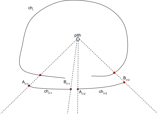
Figure 15: Endpoint condition check. See the text for an explanation.

Input: $State_{i}$,

$Ch_{j}$, // current chain

$candidate\_chain$, // chain closer to $Ch_{j}$

$Ch_{i}$, // support chain of $Ch_{j}$ and $candidate\_chain$

$endpoint$, // $Ch_{j}$ endpoint

Output: a boolean indicating if conditions are met, $distribution\_distance$ (radial difference between both chains)

/* Parameter extraction, from Table 1 */

1 $th\_radial\_tolerance$ $\leftarrow$ $State_{i}.th\_radial\_tolerance$

2 $th\_distribution\_size$$\leftarrow$$State_{i}.th\_distribution\_size$

3 $th\_regular\_derivative$$\leftarrow$$State_{i}.th\_regular\_derivative$

4 $derivative\_from\_center$$\leftarrow$$State_{i}.derivative\_from\_center$

5

/* Condition checks */

6 $distribution\_distance$ $\leftarrow$ None

7

8$size\_condition$ $\leftarrow$ $Ch_{j}.size$ + $candidate\_chain.size$ $\leq$ Nr

9

10$endpoint\_conditions$ $\leftarrow$ check_endpoints($Ch_{i},Ch_{j},candidate\_chain,endpoint$)

11

12$similarity\_condition$, $distribution\_distance$ $\leftarrow$ similarity_conditions($State_{i}$, $th\_radial\_tolerance$,$th\_distribution\_size$, $th\_regular\_derivative$, $derivative\_from\_center$, $Ch_{i}$, $Ch_{j}$, $candidate\_chain$, $endpoint$) // Equation 9

13

14$check$ $\leftarrow$ $size\_condition$ and $endpoint\_condition$ and $similarity\_condition$

15

return $check$, $distribution\_distance$

Algorithm 18 connectivity_goodness_condition

postprocessing

This last stage aims to complete the remaining chains relaxing the conditions even more. At this stage, many chains are closed, i.e., chains with $size=Nr$, which we call rings. We have some nonclosed chains that can be noisy or be part of a ring but have not been completed for some reason. We use the information on the neighborhood chains to finish or discard these remaining chains. We talk about region to describe the area between two rings.

1. It can remain some chains belonging to the same ring but not forming a closed chain. In many cases, this is due to small overlapping between chains. To solve this problem, we cut the overlapping chains in such a way as to avoid intersections between them and then try to reconnect the resulting chains that respect the connectivity goodness conditions. Figure 16 illustrates the problem.

2. Given two closed chains which contain a set of chains between them. Suppose the added angular length of the non-overlapping chains between the rings is more significant than 180 degrees. In that case, we consider that those uncompleted chains have enough information about the ring, so we complete it. The completion is based on the interpolation between both rings and the location of the existing chains. The chains that become part of the closed chain are the ones that meet the connectivity goodness conditions.

3. To test the connectivity goodness in this stage, we use the values on the last column of Table 1.

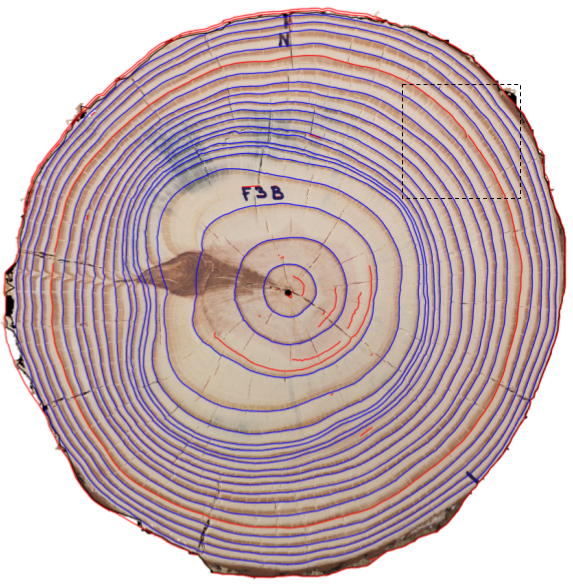
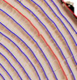
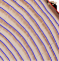
Figure 16: a) F03d disk after connecting stage. b) There is a ring that cannot be closed because of chain intersection issues. c) Ring is closed after the postprocessing stage.

The method is described by Algorithm 19. It uses the center of the spider web and the chains and nodes lists. In line 1, the function is initialized,

• $l\_ch_{c}$ is copied into new list $l\_ch_{p}$

• Function variables are initialized as $chain\_was\_completed=FALSE$, $idx\_start=NONE$

The main loop spans all the closed chains and includes lines 2 to 14. In line 3, the DiskContext object is instantiated. This object handles the logic to iterate over the regions delimited by the closed chains and go from the smaller to the bigger area (defined between the chain and the center). The two neighboring closed chains, and all the chains between them are identified in line 5 (ctx.update()). Some information is stored in the following variables

• $inward\_ring$: The inward closed chain. If it is the first iteration, the chain is of type center (an artificial chain in the center with $area=0$).

• $outward\_ring$: The outward closed chain. If the chain is of type border, this is the last iteration.

• $l\_within\_chains$: chain subset delimited by $inward\_ring$ and $outward\_ring$.

A ring defines an internal area from the chain to the center. All closed chains (rings) are sorted by their inner area. The current index iteration is stored in the variable idx of object DiskContext.

The shapely python library is used to get the chains in regions between two rings. A region is determined by two shapely Polygon, one external and one internal. A Polygon is a list of points. Each closed chain is codified as a shapely Polygon. A method of the object Polygon allows us to find the set of uncompleted chains inside a region.

The loop defined between lines 4 and 12 iterates over the closed chains. In line 6, the function for split and connect chains is called. If a chain inside $l\_within\_chains$ is closed during the call to ${split\_and\_connect\_chains}$, we exit the inner loop. If a chain was completed during a call, $chain\_was\_completed$ is set to TRUE in line 6. The next iteration will work with the same $inward\_ring$, but the formerly closed chain is used as $outward\_ring$. The set $l\_within\_chains$ is modified accordingly. In line 8, $idx\_start$ variable is set for the DiskContext object in the next iteration.

The chains are connected if enough information between inward and outward chains and connectivity goodness conditions are met (line 10). In line 15, all the chains with enough nodes (more than $0.95Nr$ nodes) are closed. In that case, new nodes are added to obtain a chain with Nr nodes. To this aim, we linearly interpolate between the inward and outward rings, going from one endpoint to another. Finally, the list of all post-processed chains, both closed and not closed, $l\_ch_{p}$ is returned.

Input: $l\_ch_{c}$, // chains list

$l\_nodes_{c}$, // nodes list

$c$ // center of the sypder web

Output: A list of post-processed chains $l\_ch^{k}_{p}$, $k=1,2,\cdots,N_{f}$

1 $l\_ch_{p}$ $\leftarrow$ initialization($l\_ch_{c}$)

2 while True do

3       ctx $\leftarrow$ DiskContext($l\_ch_{p}$, $idx\_start$)

4       while $len(ctx.completed\_chains)>0$ do

5             $l\_within\_chains$, $inward\_ring$, $outward\_ring$ $\leftarrow$ ctx.update()

6             $chain\_was\_completed$ $\leftarrow$ split_and_connect_chains($l\_within\_chains$, $inward\_ring$, $outward\_ring$, $l\_ch_{p}$, $l\_nodes_{c}$,$ctx.neighbourhood\_size$) // See Algorithm 20

7             if chain_was_completed then

8                   idx_start $\leftarrow$ ctx.idx

9                   break

10                  

11            connect_chains_if_there_is_enough_data($ctx$, $l\_nodes_{c}$, $l\_ch_{p}$)

12             if ctx.exit() then

13                   break

14                  

15            

16      if not $chain\_was\_completed$ then

17            break

18            

19      

20complete_chains_if_required($l\_ch_{p}$)

return $l\_ch_{p}$

Algorithm 19 Posprocessing Main Logic

The method ${split\_and\_connect\_chains}$ is described in Algorithm 20. It iterates over all the chains within a region to connect them. At every chain endpoint, the method cuts all the chains that intersect the ray passing through that endpoint and checks the connectivity goodness condition, Equation 8, between the divided chains to find connections between them. Notice that this module removes the chain overlapping constraint. The parameters used by this module are:

1. $neighbourhood\_size$ = 45

2. $Th_{Radial\_tolerance}$ = 0.2

3. $Th_{Distribution\_size}$ = 3

4. $Th_{Regular\_derivative}$ = 2

The parameter $neighbourhood\_size$ defines the maximum angular distance (Equation 7) to consider candidate chains departing from an endpoint in both directions. Given a source chain (the current chain $Ch_{j}$), every chain in the region that overlaps $Ch_{j}$ in more than $neighbourhood\_size$ is not considered a candidate chain to connect because if there is a very long overlapping, that chain is probably part of another ring. In line 1, the method is initialized, and variables $connected$, $completed\_chain$, and $Ch_{j}$ are set to FALSE. Also, the chains in $l\_within\_chains$ list are sorted by size in descending order. The chain nodes inside the region are stored in the $l\_inward\_nodes$ list (line 2). The main loop, lines 3 to 15, iterates over the chains in $l\_within\_chains$. The loop terminates when either current chain $Ch_{j}$ is closed or all chains in list $l\_within\_chains$ have been tested. In line 10, a new (non-treated) chain is extracted for the current iteration and stored in $Ch_{j}$. The splitting and connecting logic called $split\_and\_connect\_neighbouring\_chains$ is executed in line 13. The best candidate chain for endpoint A ($Ch_{k}^{a}$) is determined at this point, while the best candidate chain for endpoint B ($Ch_{k}^{b}$) is obtained in line 14. $Ch_{i}^{a}$ and $Ch_{i}^{b}$ are the support chains of chains $Ch_{k}^{a}$ and $Ch_{k}^{b}$ respectively. The radial distance (Equation 6) of chain $Ch_{k}^{a}$($Ch_{k}^{b}$) to $Ch_{j}$ trough endpoint $A$($B$) is $diff_{a}$($diff_{b}$). The radially closest candidate chain is connected in function $connect\_radially\_closest\_chain$ (line 15), and the maximum number of nodes ($Nr=360$) constraint is verified. The same node interpolation as in line 15 of Algorithm 19 is used.

Input: $l\_within\_chains$, // uncompleted chains delimited by inward_ring and outward_ring

$inward\_ring$, // inward ring of the region

$outward\_ring$, // outward ring of the region

$l\_ch_{p}$, // chain list

$l\_nodes_{c}$, // full nodes list

Parameter:

$neighbourhood\_size$ // size to search for chains that intersect the other endpoint

Output: boolean value indicating if a chain has been completed on the region

1 $connected$, $completed\_chain$, $Ch_{j}$ $\leftarrow$ initialization_step($l\_within\_chains$)

2 $l\_inward\_nodes$ $\leftarrow$ get_nodes_from_chain_list($l\_within\_chains$)

3 while True do

4       if not $connected$ then

5            

6            if $Ch_{j}$ is not None and $Ch_{j}.is\_closed()$ then

7                   complete_chain_using_2_support_ring($inward\_ring$, $outward\_ring$, $Ch_{j}$)

8                   completed_chain $\leftarrow$ True

9                   $Ch_{j}$ $\leftarrow$ None

10                  

11            else

12                   $Ch_{j}$ $\leftarrow$ get_next_chain( $l\_within\_chains$)

13                  

14            

15      if $Ch_{j}$ == None then

16            break

17      $Ch_{k}^{a}$, $diff\_a$, $Ch_{i}^{a}$ $\leftarrow$ split_and_connect_neighbouring_chains($l\_inward\_nodes$, $l\_within\_chains$, $Ch_{j}$, $A$, $outward\_ring$, $inward\_ring$, $neighbourhood\_size$)

18      

19      $Ch_{k}^{b}$, $diff\_b$, $Ch_{i}^{b}$ $\leftarrow$ split_and_connect_neighbouring_chains($l\_inward\_nodes$, $l\_within\_chains$, $Ch_{j}$, $B$, $outward\_ring$, $inward\_ring$, $neighbourhood\_size$, $aux\_chain=Ch_{k}^{a}$)//See Algorithm 21

20      

21      $connected$, $Ch_{i}$, $endpoint$ $\leftarrow$ connect_radially_closest_chain($Ch_{j}$, $Ch_{k}^{a}$, $diff\_a$, $Ch_{i}^{a}$, $Ch_{k}^{b}$, $diff\_b$, $Ch_{i}^{b}$, $l\_ch_{p}$, $l\_within\_chains$, $l\_nodes_{c}$, $inward\_ring$, $outward\_ring$)

22      

return $completed\_chain$

Algorithm 20 split_and_connect_chains

Given a source chain, $Ch_{j}$, the logic for splitting neighborhood chains and searching for candidates is implemented by Algorithm 21. Chains that intersect the ray supporting $Ch_{j}$ endpoint are split. In line 1, the angle domain of $Ch_{j}$ is stored in $Ch_{j}\_angle\_domain$. In line 2, variable $Ch_{j}\_node$ stores the $Ch_{j}$ node endpoint. The closest chain ring to the $Ch_{j}$ endpoint (in Euclidean distance) is selected as the support chain, $Ch_{i}$. From lines 4 to 7, we have the logic to get all chains in the region delimited by two rings intersecting the ray $Ray_{e}$ supporting the endpoint. First, we store in $l\_nodes\_ray$ all the nodes over $Ray_{e}$, pinpointing the chains supporting those nodes, and keep those chains in $l\_endpoint\_chains$. To be cut, the overlapping between a chain in the set $l\_endpoint\_chains$ and $Ch_{j}$ must be smaller than $neighbourhood\_size$. Otherwise, it is filtered because that chain belongs to another ring (line 7). The method in line 8 effectively cut the chosen chains. Once a chain is cut, it produces a $sub\_chain$ nonintersecting $Ch_{j}$, stored as a candidate chain in $l\_candidates$ (line 8) and in the list $l\_no\_intersections\_j$ (line 9). In line 10, all chains that intersect $Ch_{j}$ in the second endpoint and are in the neighborhood of the first endpoint are added to $l\_candidates$. Also, the chains in the $Ch_{j}$ chain neighborhood, which does not intersect its endpoint but intersects in the other endpoint, are split (line 11). In line 12, all chains in $l\_no\_intersections\_j$ that are far away in terms of angular distance (Equation 7) from the given endpoint of $Ch_{j}$ are removed. The nonintersecting chains in the endpoint neighborhood are stored in $l\_filtered\_no\_intersection\_j$. In line 13, chains in $l\_filtered\_no\_intersection\_j$ are added to $l\_candidates$. In line 14, all chains from $l\_candidates$ which do not satisfy the connectivity goodness conditions of Equation 8 are discarded. In line 15, the closest chain that meets the connectivity goodness conditions is returned, $Ch_{k}$, and $diff$, the radial difference between $Ch_{k}$ and $Ch_{j}$ endpoints(Equation 6), and the support chain, $Ch_{i}$.

Input: $l\_within\_nodes$, // nodes within region

$l\_within\_chain$, // uncompleted chains delimited by inward and outward rings

$Ch_{j}$, // current source chain. The one that is being connected if conditions are met

$endpoint$,// endpoint of source chain to find candidate chains to connect

$outward\_ring$, // outward support chain ring

$inward\_ring$, // inward support chain ring

$neighbourhood\_size$, // total nodes size to search for chains that intersect the other endpoint

Output: Source chain $Ch_{k}$, $radial\_distance$ and closest support chain to endpoint, $Ch_{i}$

1

2$Ch_{j}\_angle\_domain$ $\leftarrow$ get_angle_domain($Ch_{j}$)

3 $Ch_{j}\_node$ $\leftarrow$ get_node_endpoint($Ch_{j}$,$endpoint$)

4 $Ch_{i}$ $\leftarrow$ select_support_chain($outward\_ring$, $inward\_ring$, $Ch_{j}\_node$)

5 $l\_nodes\_ray$ $\leftarrow$ select_nodes_within_region_over_ray($Ch_{j}$, $Ch_{j}\_node$, $l\_within\_nodes$)

6 $l\_chain\_id\_ray$$\leftarrow$extract_chains_ids_from_nodes($l\_nodes\_ray$)

7 $l\_endpoint\_chains$ $\leftarrow$ get_chains_from_ids($l\_within\_chains$, $l\_chain\_id\_ray$)

8

9$l\_filtered\_chains$ $\leftarrow$ remove_chains_with_higher_overlapping_threshold($Ch_{j}\_angle\_domain$, $l\_endpoint\_chain$,$neighbourhood\_size$)

10 $l\_candidates$ $\leftarrow$ split_intersecting_chains($Ch_{j}\_node.angle$, $l\_filtered\_chains$, $Ch\_j$)//See Algorithm 22

11 $l\_no\_intersections\_j$ $\leftarrow$ get_chains_that_no_intersect_src_chain($Ch_{j}$, $Ch_{j}\_angle\_domain$, $l\_within\_chains$,$l\_endpoint\_chains$)

12 add_chains_that_intersect_in_other_endpoint($l\_within\_chains$, $l\_no\_intersections\_j$, $l\_candidates$, $Ch_{j}$, $neighbourhood\_size$, $endpoint$)

13 $l\_candidates$ $\leftarrow$ split_intersecting_chain_in_other_endpoint($endpoint$, $Ch_{j}$, $l\_within\_chains$, $l\_within\_nodes$, $l\_candidates$)

14 $l\_filtered\_no\_intersection\_j$ $\leftarrow$ filter_no_intersected_chain_far($l\_no\_intersections\_j$, $Ch_{j}$, $endpoint$, $neighbourhood\_size$)

15 $l\_candidates$ $\leftarrow$ $l\_candidates$ + $l\_filtered\_no\_intersection\_j$

16 $l\_ch_{k}\_Euclidean\_distances$, $l\_ch_{k}\_radial\_distances$, $l\_ch_{k}$ $\leftarrow$  get_chains_that_satisfy_similarity_conditions($Ch_{i}$, $Ch_{j}$, $\_candidates$, $endpoint$)

17 $Ch_{k}$, $diff$ $\leftarrow$ select_closest_candidate_chain($l\_ch_{k}$, $l\_ch_{k}\_Euclidean\_distances$, $l\_ch_{k}\_radial\_distances$, $l\_within\_chains$, $aux\_chain$)

return $Ch_{k}$,$diff$,$Ch_{i}$

Algorithm 21 split_and_connect_neighbouring_chains

Method $split\_intersecting\_chains$ is described in Algorithm 22. Given an endpoint ray direction, we iterate over all the intersecting chains in that $direction$. Given a chain to be split, $inter\_chain$, and the node, $split\_node$, we divide the chain nodes in two chains cutting the nodes list in the position of $split\_node$. Remember that the list of nodes within a chain is clockwise sorted. After splitting the chain in $sub\_ch1$ and $sub\_ch2$, we select the sub chain that does not intersect $inter\_chain$, line 5. Then, if $Ch_{k}$ intersects $Ch_{j}$ in the other endpoint, this means that $inter\_chain$ intersects $Ch_{j}$ at both endpoints, we repeat the logic over the other endpoint but for $Ch_{k}$ instead of $inter\_chain$. The split chain list is returned in $l\_search\_chains$.

Input: $direction$, // endpoint direction for split chains

$l\_filtered\_chains$, // list of chains to be split

$Ch_{j}$, // source chain. The one that is being to connect if conditions are met

Output: split chain list

1 $l\_search\_chains$ $\leftarrow$ []

2 for $inter\_chain$ in $l\_filtered\_chains$ do

3       $split\_node$ $\leftarrow$get_node_by_angle($direction$)

4       $sub\_ch1$, $sub\_ch2$ $\leftarrow$ split_chain($inter\_chain$, $split\_node$)

5       $Ch_{k}$ $\leftarrow$ select_no_intersection_chain_at_endpoint($sub\_ch1$, $sub\_ch2$, $Ch_{j}$, $direction$)

       /* Longest chains intersect two times */

6       if intersection_between_chains($Ch_{k}$, $Ch_{j}$) then

7             $split\_node\_2$ $\leftarrow$ get_node_by_angle($node\_direction\_2$)

8             $sub\_ch1$, $sub\_ch2$ $\leftarrow$ split_chain($Ch_{k}$, $split\_node\_2$)

9             $Ch_{k}$ $\leftarrow$ select_no_intersection_chain_at_endpoint($sub\_ch1$, $sub\_ch2$, $Ch_{j}$, $node\_direction\_2$)

10            

11      change_id($Ch_{k}$)

12       $l\_search\_chains$ $\leftarrow$ $l\_search\_chains$ + $Ch_{k}$

13      

return $l\_search\_chains$

Algorithm 22 split_intersecting_chains

Another critical method from Algorithm 19 is $connect\_chains\_if\_there\_is\_enough\_data$. When there is a unique chain longer than $information\_threshold$ ($180$ in our experiments), we interpolate between its endpoints using both inward and outward support chains. When there are several chains in the region, we get the largest subset of chains in the region that non intersect each other. Suppose the chains over this subset have an angular domain bigger than $information\_threshold$ (180 in our experiments). In that case, we iterate over the chains within the subset (sorted by size) and connect all the chains that satisfy the similarity condition using the last column of Table 1.

3.3 Pith detection

The pith position is an input for the method. In the demo it can be set manually or using the method proposed for Decelle et al, [4], which is at the IPOL site.

4 Implementation

The implementation was made in Python 3.11.

4.1 Input and Output

The demo requires as input, a segmented image and the pith position. A command line execution example is:

⬇

$ python main.py –input IMAGE_PATH –cx CX –cy CY

–output_dir OUTPUT_DIR –root REPO_ROOT_DIR

As output, the method returns a JSON file with the tree-rings position in Labelme format [23].

The parameters of the program are the following:

• –input: path to the segmented image.

• –cx: pith x’s coordinate.

• –cy: pith y’s coordinate.

• –output_dir: directory where intermediate and final results are saved.

• –root: repository root path

4.2 Parameters

Table 2 summarises parameters that the user can modify if needed. Program command line parameters are the following:

• –sigma: Gaussian filtering standard deviation $\sigma$.

• –th_low: Low threshold on the gradient module for the Canny Devernay filter.

• –th_high: High threshold on the gradient module for the Canny Devernay filter.

• –height: image height after the resizing process.

• –width: image width after the resizing process.

• –alpha: threshold on the collinearity of the edge filtering (Equation 3).

• –nr: total number of rays.

• –min_chain_lenght: minimun chain lenght.

	stage	Parameter	Default
Basic	edges detector	Gaussian filtering $\sigma$	3
	preprocessing	height	None
		width	None
	filtering, sampling, connect	Pith Position	Required
Advanced	edges detector	Gradient threshold low	5
		Gradient threshold high	15
	edges filtering	collinearity threshold ($\alpha$)	30°
	sampling	rays number (nr)	360
		min chain length	2

Table 2: Method parameters. Basic parameters can be modified by the user in the demo.

4.3 Installation and Use

The main program language is Python. However, the edge detector stage uses the code in C from IPOL ([10]) and must be compiled. The source code is included in our repository because some minor modifications were made to extract the image gradient.

The procedure to install the application is the following:

⬇

$ cd repo_root/

⬇

$ apt-get update && apt-get install -y $(cat .ipol/packages.txt) &&

rm -rf /var/lib/apt/lists/*

⬇

$ pip3 install –no-cache-dir -r requirements.txt

⬇

$ cd ./externas/devernay_1.0 && make clean && make

5 Datasets

To test the proposed method, we use two datasets:

1. The UruDendro dataset. An online database [16] with images of cross-sections of commercially grown Pinus taeda trees from northern Uruguay, ranging from 13 to 24 years old, composed of twelve individual trees collected in February 2020 in Uruguay. Six trees correspond to a lumber company (denoted by the letter F), and the other six correspond to a plywood company (denoted by the letter L). Each company applied different silviculture practices. The individuals were identified by the letter of the company, a two-digit number, and a lowercase letter corresponding to the height where each cross-section was obtained. Heights were coded as follows: a = 10 cm above the ground, b = 165 cm, c = 200 cm, d = 400 cm, and e = 435 cm. The cross-sections were about 5 to 20 cm thick and were dried at room temperature without further preparation. As a consequence of the drying process, radial cracks and blue fungus stains were developed in the cross-sections. Surfaces were smoothed with a handheld planer and a rotary sander. Photographs were taken under different lighting conditions; cross-sections a, b, and e were photographed indoors and moistened to maximize contrast between early- and late-wood. Pictures of dry cross-sections c and d were taken outdoors. The dataset has 64 images of different resolutions, described in Table 4. The collection contains several challenging features for automatic ring detection, including illumination and surface preparation variation, fungal infection (blue stains), knot formation, missing bark and interruptions in outer rings, and radial cracking. The proposed CS-TRD tree-ring detection method was checked against manual delineation of all rings by users of varying expertise using the Labelme tool [23]. At least two experts annotate all images. Figure 2 show some images in this UruDendro dataset.

2. The Kennel dataset. Kennel et al. [13] made available a public dataset of 7 images of Abies alba and presented a method for detecting tree rings. We were unable to process the annotations given by the authors. The characteristics of this dataset are described in Table 3. We label the dataset with the same procedure as the UruDendro dataset to evaluate the results.

Table 3: The Kennel dataset, are signaled the name and dimensions of each image as well as the number of expert marks and the number of rings in each one.

Image	Marks	Rings	Height (pixels)	Width (pixels)
AbiesAlba1	4	52	1280	1280
AbiesAlba2	2	22	1280	1280
AbiesAlba3	3	27	1280	1280
AbiesAlba4	1	12	1024	1024
AbiesAlba5	3	30	1280	1280
AbiesAlba6	2	21	1280	1280
AbiesAlba7	1	48	1280	1280

Table 4: The UruDendro dataset, are signaled the name and dimensions of each image as well as the number of expert marks and the number of rings in each one.

Image	Marks	Rings	Height (pixels)	Width (pixels)
F02a	2	23	2364	2364
F02b	2	22	1644	1644
F02c	4	22	2424	2408
F02d	2	20	2288	2216
F02e	2	20	2082	2082
F03a	2	24	2514	2514
F03b	2	23	1794	1794
F03c	1	24	2528	2596
F03d	1	21	2476	2504
F03e	3	21	1961	1961
F04a	2	24	2478	2478
F04b	1	23	1760	1762
F04c	3	21	913	900
F04d	2	21	921	899
F04e	1	21	2070	2072
F07a	1	24	2400	2400
F07b	3	23	1740	1740
F07c	1	23	978	900
F07d	1	22	997	900
F07e	1	22	2034	2034
F08a	3	24	2383	2383
F08b	2	23	1776	1776
F08c	2	23	2624	2736
F08d	2	22	2388	2400
F08e	2	22	1902	1902
F09a	1	24	2106	2106
F09b	4	23	1858	1858
F09c	1	24	2370	2343
F09d	1	23	2256	2288
F09e	1	22	1610	1609
F10a	2	22	2136	2136
F10b	2	22	1677	1677
F10e	1	20	1800	1800
L02a	1	16	2088	2088
L02b	3	15	1842	1842
L02c	1	13	1016	900
L02d	2	14	921	900
L02e	2	14	1914	1914
L03a	2	17	2296	2296
L03b	2	16	2088	2088
L03c	2	16	2400	2416
L03d	2	16	2503	2436
L03e	2	14	1944	1944
L04a	4	17	2418	2418
L04b	2	16	1986	1986
L04c	2	16	2728	2704
L04d	2	16	2544	2512
L04e	1	15	1992	1992
L07a	2	17	2328	2328
L07b	2	16	2118	2118
L07c	3	17	2492	2481
L07d	1	16	2480	2456
L07e	2	15	1980	1980
L08a	2	17	2268	2268
L08b	2	16	1836	1836
L08c	1	16	2877	2736
L08d	2	14	2707	2736
L08e	1	15	1666	1666
L09a	1	17	1963	1964
L09b	3	16	1802	1802
L09c	1	16	943	897
L09d	2	15	1006	900
L09e	1	15	1662	1662
L11b	4	16	1800	1800

6 Experiments and Results

6.1 Metric

To evaluate the method, we develop a metric based on the one proposed by Kennel et al., [13]. To say if a ring is detected, we define an influence area for each ring as the set of pixels closer to that ring. For each ray, the frontier is the middle point between the nodes of consecutive ground truth rings. Figure 17.b show the influence area for disk F03d. Each ground truth ring is colored in black and is the center of its influence area. Figure 17.a shows the red detections and the green ground truth marks for the same image.

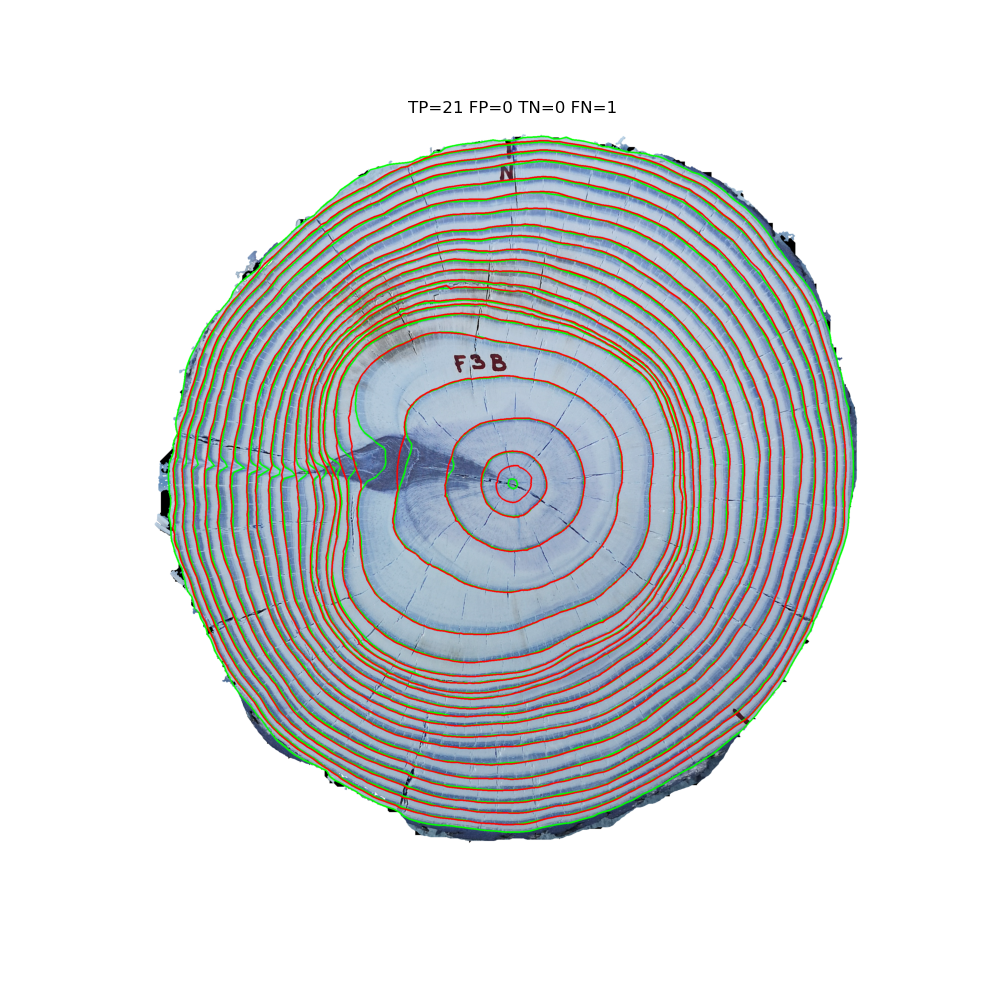
(a)

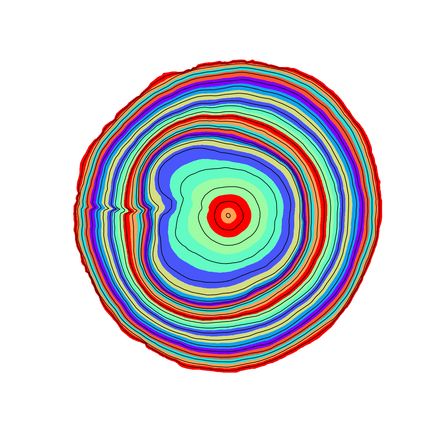
(b)

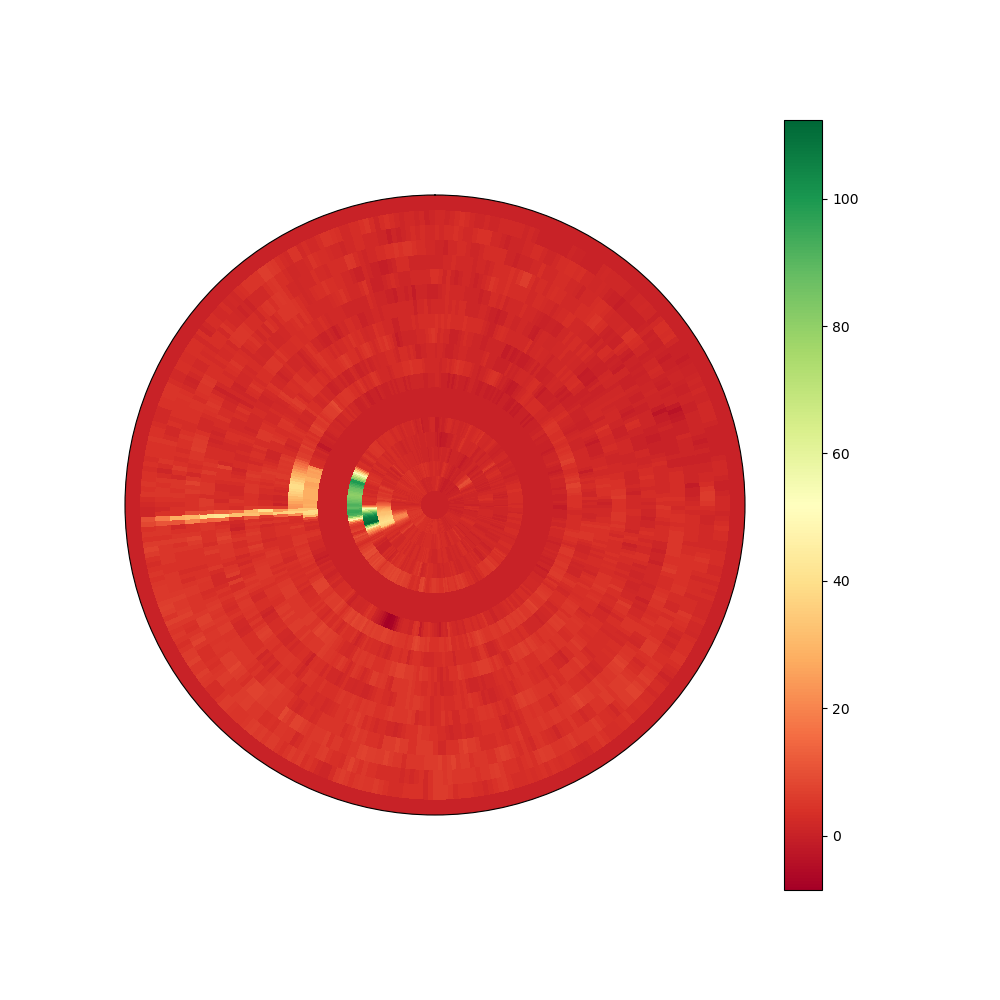
(c)

Figure 17: Measuring the error between automatic detection and the ground truth for image F03d. (a): In green, the ground truth; in red, the marks produced by the method (detections). (b): Areas of influence of the ground truth rings. (c): Error, in pixels, between the detection and the ground truth.

The influence area associates a detected curve with a ground truth ring. In both cases, the nodes are associated with the $Nr$ rays. Given a ground truth ring, we assign it to the closest detection using:

$$Dist=\sqrt{\frac{1}{Nr}\sum_{i=0}^{Nr-1}\left(dt_{i}-gt_{i}\right)^{2}}\hskip 14.22636pt$$ (10)

Where $i$ represents the ray direction, $dt_{i}$ is the radial distance ( Equation 6) of detected node $i$, and $gt_{i}$ is the radial distance ( Equation 6) of the corresponding ground truth node $i$.

The closest detection can be extremely far away. To assign a detected curve to a ground truth ring, we must guarantee that the given chain is the closest one to the ring and that it is close enough. To this aim, we use the influence area of each ground truth ring (see Figure 17). Given a detected curve, we compute the proportion of nodes of that chain that belongs to the influence region of the closest ring. If that measure exceeds a parameter ($th\_pre=60\%)$, we assign the detected curve to the ground truth ring. If not, the detected curve is not assigned to any ground truth ring. In other words, at least $60\%$ of the nodes of a detected curve must be in the influence area of the ground truth ring to be assigned to it and to say that we have detected that ring (hence to declare a true positive).

Figure 17.c show the error in pixels between the ground truth rings and the detected curves assigned to them. The red color represents a low error, while the yellow-green color represents a high error. Note how the error is concentrated around the knoth, which perturbs the precise detection of some rings.

Once all the detected chains are assigned to the ground truth rings, we calculate the following indicators:

1. True Positive (TP): if the detected closed chain is assigned to the ground truth ring.

2. False Positive (FP): if the detected closed chain is not assigned to a ground truth ring.

3. False Negative (FN): if a ground truth ring is not assigned to any detected closed chain.

Finally, the Precision measurement is given by $P=\frac{TP}{TP+FP}$, the Recall measurement by $R=\frac{TP}{TP+FN}$ and the F-Score by $F=\frac{2PR}{P+R}$.

Results for the Kennel dataset are shown in Table 6 and for the UruDendro dataset in Table 7. For example, in the image F03d, the method fails to detect two ground truth rings, so $FN=2$. The other rings are correctly detected. The table also shows the execution time for each image and the RMSE error( Equation 10) between the detected and ground truth rings.

6.2 Experiments

This section presents some experiments to understand the method and its limitations better. At the end of the section, an experiment shows the dependence of the results with the threshold $th\_pre$. All experiments were made using a workstation with Intel Core i5 10300H and RAM 16GB.

6.2.1 Edge detector optimization stage

The algorithm relies heavily on the edge detector stage. The first experiment tests different $\sigma$ values for the Canny Devernay edge detector to get the one that maximizes the F-Score for the dataset UruDendro. This dataset presents significant variations in image resolution and allows us to study the global performance with different dimensions of the input images. We compute the average F-Score for the original image sizes and when all the images in the dataset are scaled to several sizes: 640x640, 1000x1000, 1500x1500. Results are shown in Figure 18. The best result (average F-Score of 0.89) is obtained for size 1500x1500 and $\sigma=3.0$. The execution time varies with image size, as shown in the figure. The average execution time for the 1500x1500 size is 17 seconds. The same experiment is done over Kennel et al., [13] dataset. Results are shown in Figure 19. As before, the best F-Score is obtained for the 1500x1500 resolution, but with $\sigma=2.5$. The lower optimal $\sigma$ can be related to the Kennel dataset having images with more rings on the disk, 30 on average, while the UruDendro dataset has 19 rings per disk on average. The more the disks, the less their width. Table 5 summarizes the results of this experiment for both datasets.

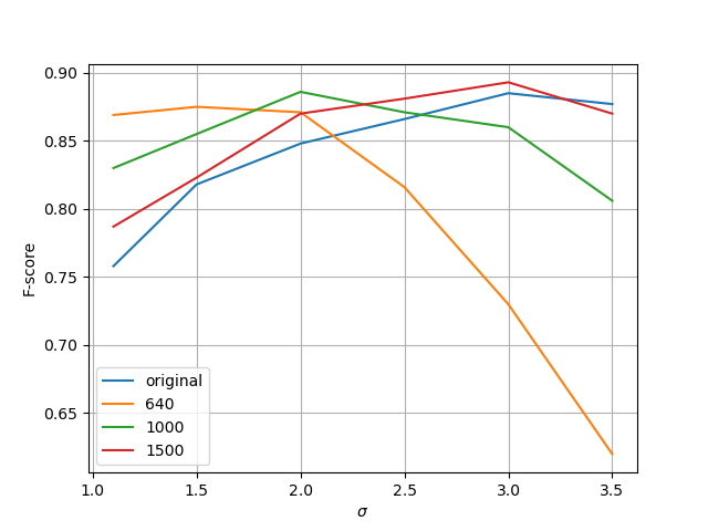
(a) Average F1 vs $\sigma$ curve for different image sizes.

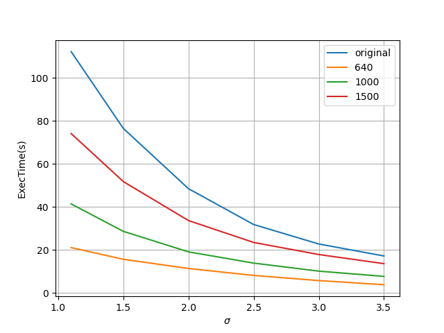
(b) Average execution time (in seconds) vs $\sigma$ curve for different images sizes.

Figure 18: Experiment results over the UruDendro dataset. Each curve represents different image sizes: 640x640, 1000x1000, 1500x1500, and original resolution. The blue curve refers to the original image size.

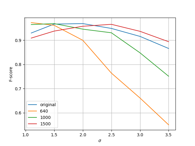
(a) Average F1 vs $\sigma$ curve for different image sizes.

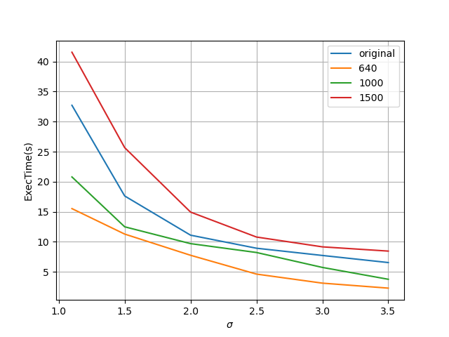
(b) Average execution time (in seconds) vs $\sigma$ curve for different image sizes.

Figure 19: Experiment results over Kennel dataset. Each curve represents a different image resolution: 640x640, 1000x1000, 1500x1500, and original resolution. The blue curve refers to the original image size.

dataset	image sizes	$\sigma$	P	R	F	RMSE	ExecTime(s)
UruDendro dataset	1500x1500	3.0	0,95	0,86	0,89	5.27	17.3
Kennel dataset	1500x1500	2.5	0,97	0,97	0,97	2.4	11.1

Table 5: Mean performance values for both datasets’ optimal image resolution.

6.2.2 Pith position sensibility

The next experiment measures how sensitive the method is to errors in the pith estimation. Figure 20 shows 48 different pith positions used in this experiment. We selected eight different pith positions over six rays. These radial displaced pith positions are selected as follows:

• Three positions are marked inside ring 1, with an error over the ray direction of 25%, 50%, and 75%.

• One is marked on ring 1.

• Three positions are marked between the first and second rings, with increasing errors of 25% over the ray direction.

• another position is marked on ring 2.

We run the algorithm for each disk with each of these pith positions, giving 48 results. We get the average RMSE and F-Score measures over the six ray directions for each radially displaced pith position, i.e., the mean for the six pith positions that are 25% off the center and so on. In this manner, we have two vectors (one for RMSE and the other for the F-Score) with eight coordinates for each one. Experiments are made over the UruDendro dataset, using an image size of 1500x1500 and $\sigma=3.0$. Figure 21(a) shows the average F-Score over the whole dataset for each error position, while Figure 21(b) shows the average RMSE over the same dataset. As was expected, F-Score decreases as the error in the pith estimation increases. Figure 21(b) shows that the RMSE is less sensitive to pith error.

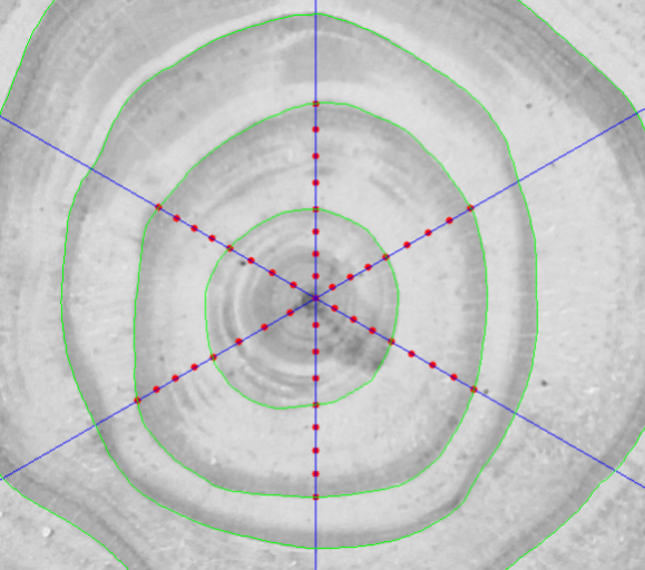
Figure 20: Pith position experiment. Given six ray directions, eight different pith positions are marked. The method is executed for each marked pith position. Ground Truth ring are marked in green

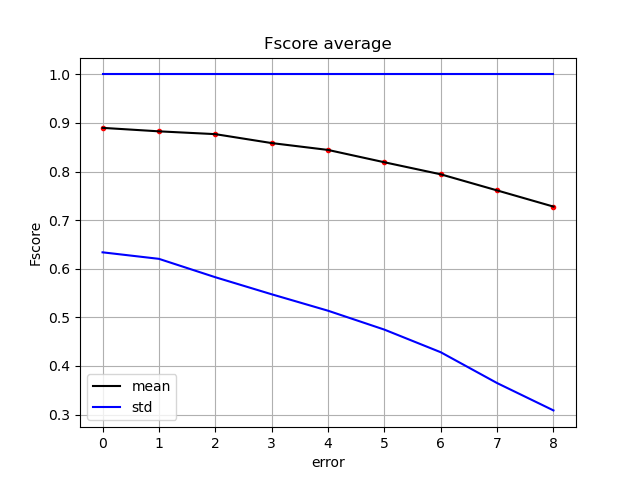
(a) Average F-Score over the UruDendro dataset.

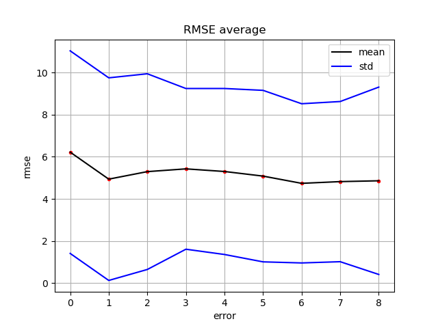
(b) Average RMSE over the UruDendro dataset.

Figure 21: For each disk of the UruDendro dataset, we run the method using the 48 different pith positions. Results are averaged over the six rays’ directions per error position.

6.2.3 Metric precision threshold

In this experiment, we see how the performance varies with different values of $th\_pre$. This parameter controls the number of nodes of the ring that lie within the Influence Area to be considered in the detection-to-ground-truth assignation step. Figure 22 and Figure 23 show results for UruDendro and Kennel datasets, respectively. As can be expected, higher precision implies higher RMSE but lower F-Score. Given these results, we fix $th\_pre=60\%$ as a default value, which seems a good compromise.

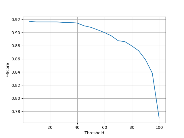
(a) Average F-Score over the UruDendro dataset.

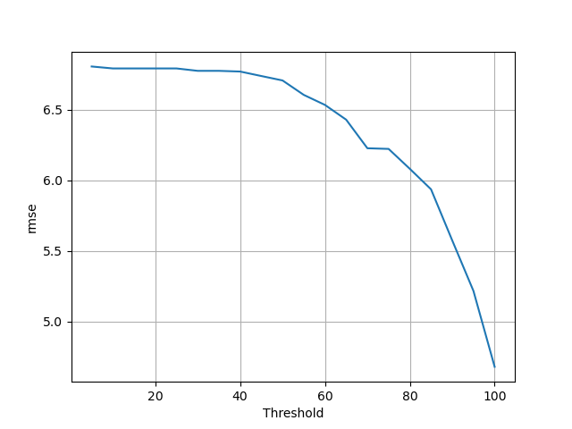
(b) Average RMSE over the UruDendro dataset.

Figure 22: Performance metrics computed for different values of $th\_pre$ parameter. UruDendro dataset.

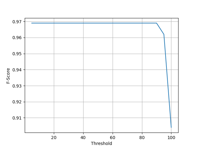
(a) Average F-Score over Kennel dataset.

(b) Average RMSE over Kennel dataset.

Figure 23: Performance metrics computed for different values of $th\_pre$ parameter on the Kennel dataset.

6.3 Results

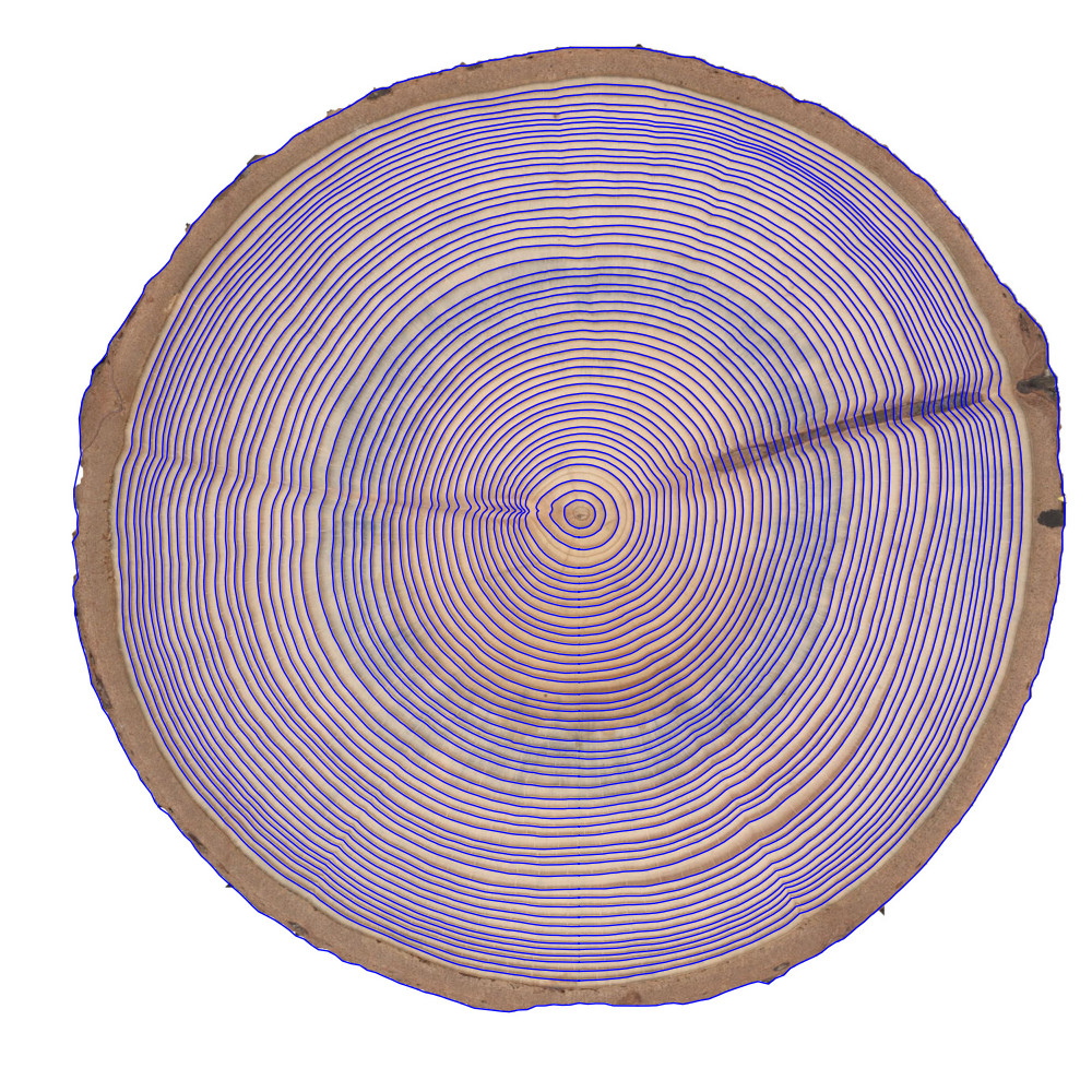
(a) AbiesAlba1

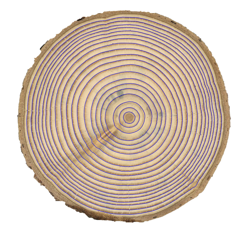
(b) AbiesAlba2

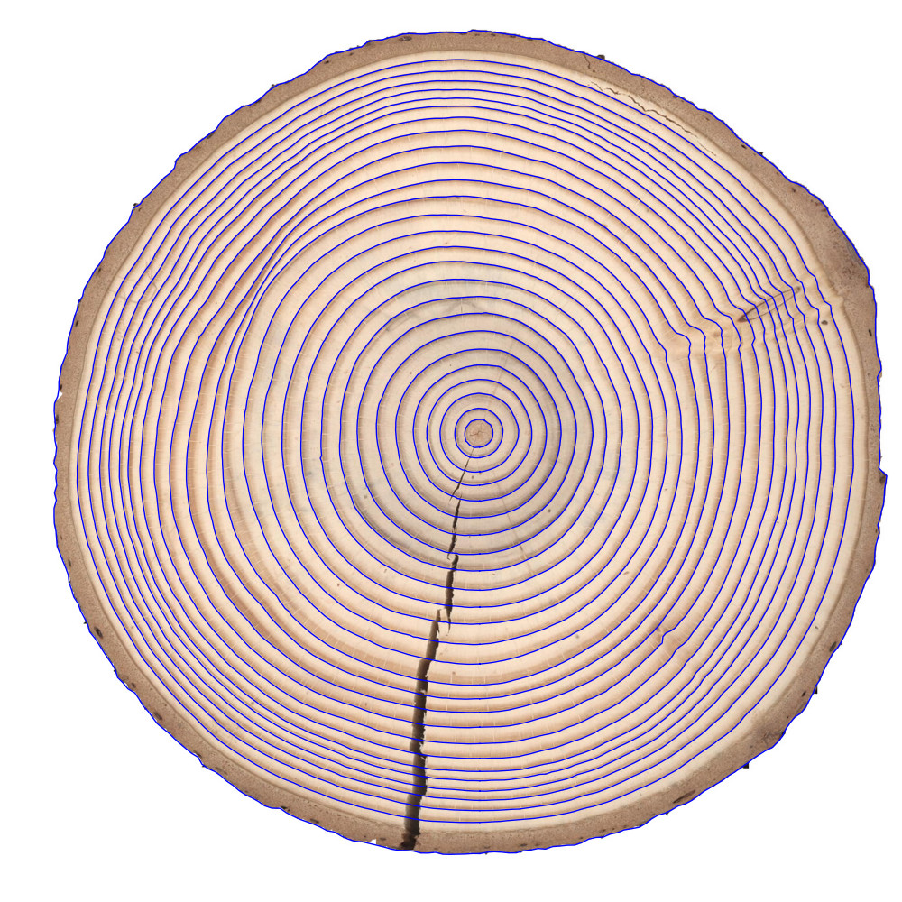
(c) AbiesAlba3

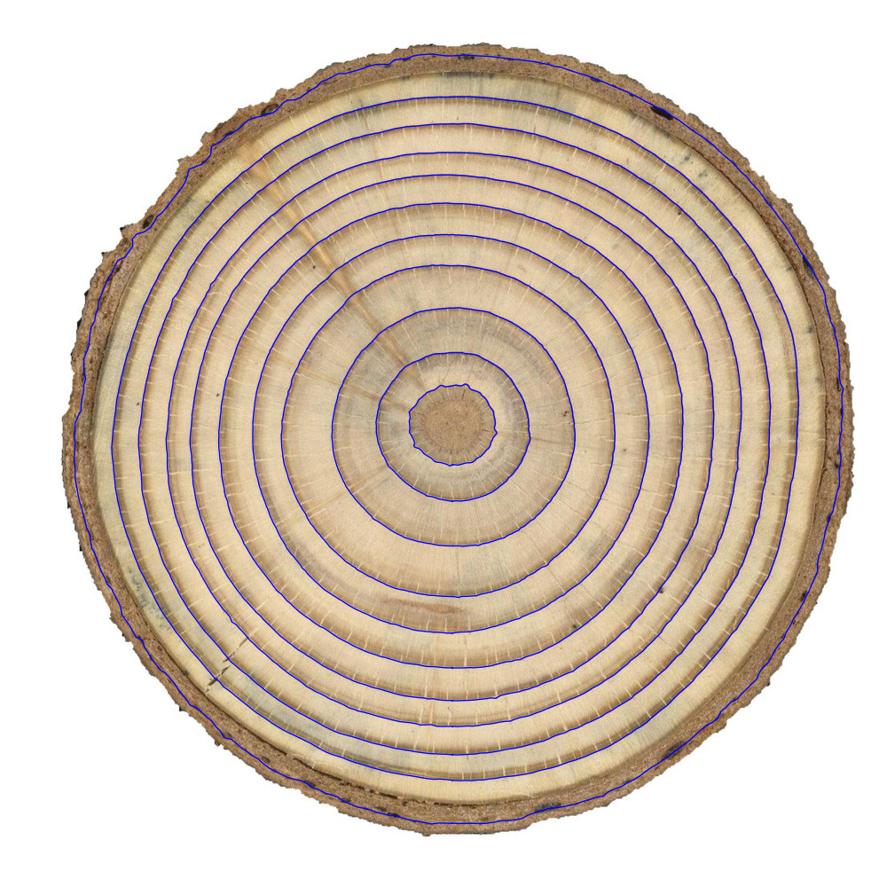
(d) AbiesAlba4

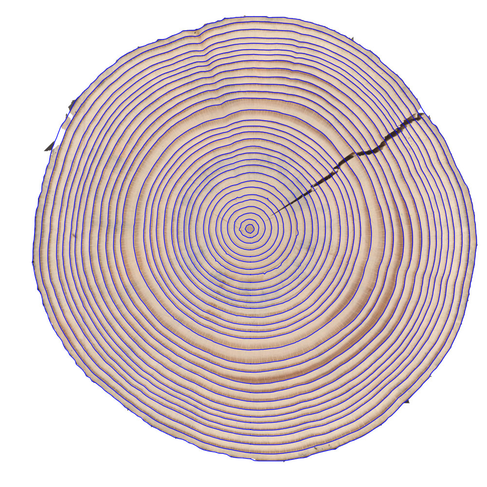
(e) AbiesAlba5

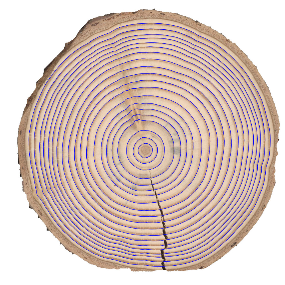
(f) AbiesAlba6

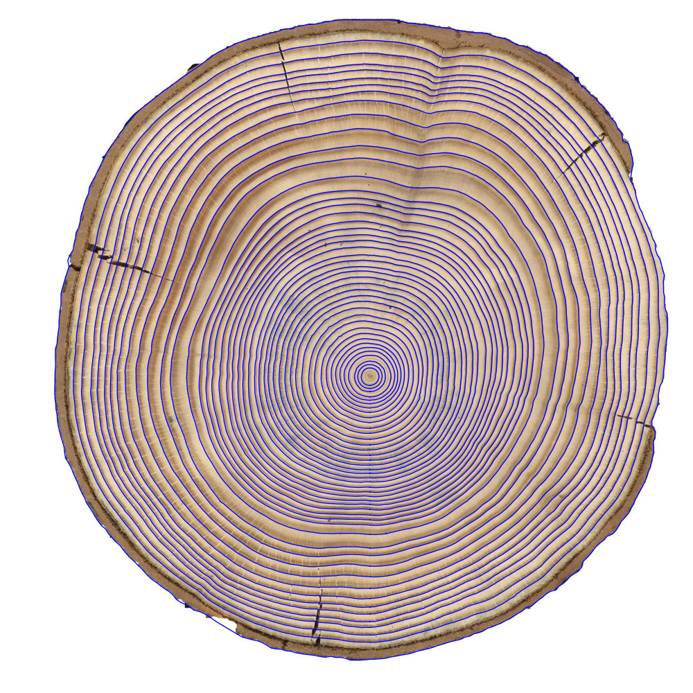
(g) AbiesAlba7

Figure 31: Results over images from the Kennel dataset with 1500x1500 image size and $\sigma=2.5$.

The results for the Kennel dataset are shown in Table 6 and Figure 31. The mean F-Score is 0.97. There are three non-detected rings per disk as a maximum. And one ring is erroneously detected per image in the worst case, generally corresponding to the border or/and the core. At Figure 24, we illustrate an example, the disk AbiesAlba1. The edge parameter is too high ($\sigma=2.5$), and the edge detector step fails to detect pith. In addition, the red chain in Figure 24.c is not closed because its size is smaller than 180 degrees (the $information\_threshold$ parameter). On the other hand, the method successfully detects the rings over the knot. Table 6 shows that the AbiesAlba1 disk has three false negatives. The third one is the last ring which is not detected, note that it detects the border and that is a false positive, as illustrated in  Figure 31.a.

(a) Filter

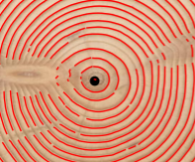
(b) Chains

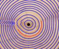
(c) Postprocessing

Figure 24: Method result for disk AbiesAlba1 (zoom in over pith center). a) Filter stage output. b) Chain stage output. c) Postprocessing stage output. At a) and b), we can see how the method fails to detect edges for pith. It is possible because the $\sigma$ threshold is too high to detect things at this resolution. At c), we can see how the red chain was not closed due to a size smaller than $information\_threshold$ (180)

The results for the UruDendro dataset are shown in Table 7. The mean F-Score is lower, 0.89, but the images in this dataset are much more complex and include knots, fungus, and cracks.

Table 6: Results on the Kennel dataset with $th\_pre=60$. Images resized to 1500x1500 and edge detector parameter $\sigma=2.5$

Name	TP	FP	TN	FN	P	R	F	RMSE	Time (sec.)
AbiesAlba1	49	1	0	3	0.98	0.94	0.96	3.66	18.01
AbiesAlba2	20	0	0	2	1.00	0.91	0.95	0.95	9.21
AbiesAlba3	26	1	0	1	0.96	0.96	0.96	1.30	8.93
AbiesAlba4	11	0	0	1	1.00	0.92	0.96	5.88	8.96
AbiesAlba5	30	1	0	0	0.97	1.00	0.98	1.29	9.06
AbiesAlba6	20	0	0	1	1.00	0.95	0.98	1.26	7.63
AbiesAlba7	45	0	0	3	1.00	0.94	0.97	3.58	13.78
Average					0.99	0.95	0.97	2.56	10.80

Table 7: Results over our dataset with $th\_pre=60\%$. Images resized to 1500x1500 and edge detector parameter $\sigma=3$.

Name	TP	FP	TN	FN	P	R	F	RMSE	Time (sec.)
F10b	19	2	0	3	0.91	0.86	0.88	4.75	20.39
F10a	17	1	0	5	0.94	0.77	0.85	4.24	15.23
F10e	18	0	0	2	1.00	0.90	0.95	2.13	12.57
F02c	21	0	0	1	1.00	0.96	0.98	3.76	12.26
F02b	21	1	0	1	0.96	0.96	0.96	4.02	13.26
F02a	20	0	0	3	1.00	0.87	0.93	1.50	15.29
F02d	20	1	0	0	0.95	1.00	0.98	2.11	8.34
F02e	20	1	0	0	0.95	1.00	0.98	7.62	23.31
F03c	23	0	0	1	1.00	0.96	0.98	10.69	7.34
F03b	20	0	0	3	1.00	0.87	0.93	2.15	13.95
F03a	22	2	0	2	0.92	0.92	0.92	8.11	19.37
F03d	19	1	0	2	0.95	0.91	0.93	7.81	11.26
F03e	20	2	0	1	0.91	0.95	0.93	1.66	15.70
F04c	18	1	0	3	0.95	0.86	0.90	5.60	26.88
F04b	19	0	0	4	1.00	0.83	0.91	4.60	40.24
F04a	21	1	0	3	0.96	0.88	0.91	7.71	28.90
F04d	17	3	0	4	0.85	0.81	0.83	2.90	55.38
F04e	19	2	0	2	0.91	0.91	0.91	9.94	24.33
F07c	20	2	0	3	0.91	0.87	0.89	4.85	35.81
F07b	17	3	0	6	0.85	0.74	0.79	7.99	45.74
F07a	18	1	0	6	0.95	0.75	0.84	11.68	18.27
F07d	20	0	0	2	1.00	0.91	0.95	1.04	19.95
F07e	8	4	0	14	0.67	0.36	0.47	8.17	40.29
F08c	21	1	0	2	0.96	0.91	0.93	2.05	13.25
F08b	21	1	0	2	0.96	0.91	0.93	1.72	23.57
F08a	21	1	0	3	0.96	0.88	0.91	5.28	17.13
F08d	20	0	0	2	1.00	0.91	0.95	2.10	9.54
F08e	22	0	0	0	1.00	1.00	1.00	6.70	17.65
F09c	21	0	0	3	1.00	0.88	0.93	2.83	9.11
F09b	22	1	0	1	0.96	0.96	0.96	2.91	11.98
F09a	21	0	0	3	1.00	0.88	0.93	2.20	16.13
F09e	14	5	0	8	0.74	0.64	0.68	7.08	38.73
L11b	15	1	0	1	0.94	0.94	0.94	1.54	10.96
L02c	11	0	0	2	1.00	0.85	0.92	5.33	21.33
L02b	4	2	0	11	0.67	0.27	0.38	9.41	21.90
L02a	14	1	0	2	0.93	0.88	0.90	16.95	26.21
L02d	7	3	0	7	0.70	0.50	0.58	5.66	28.80
L02e	11	0	0	3	1.00	0.79	0.88	4.92	18.66
L03c	15	1	0	1	0.94	0.94	0.94	9.01	8.28
L03b	15	1	0	1	0.94	0.94	0.94	2.22	10.17
L03a	14	0	0	3	1.00	0.82	0.90	3.45	16.20
L03d	14	0	0	1	1.00	0.93	0.97	10.63	8.26
L03e	13	0	0	1	1.00	0.93	0.96	3.97	14.96
L04c	14	0	0	2	1.00	0.88	0.93	3.30	8.26
L04b	15	0	0	1	1.00	0.94	0.97	6.35	10.66
L04a	15	0	0	2	1.00	0.88	0.94	6.21	7.98
L04d	14	1	0	2	0.93	0.88	0.90	7.88	6.19
L04e	10	1	0	5	0.91	0.67	0.77	4.09	10.14
L07c	14	1	0	3	0.93	0.82	0.88	2.41	5.56
L07b	13	0	0	3	1.00	0.81	0.90	6.56	9.01
L07a	13	1	0	4	0.93	0.77	0.84	1.89	13.96
L07d	14	0	0	2	1.00	0.88	0.93	1.73	5.22
L07e	11	0	0	3	1.00	0.79	0.88	13.26	17.80
L08c	15	0	0	1	1.00	0.94	0.97	2.52	8.74
L08b	14	1	0	2	0.93	0.88	0.90	11.99	24.48
L08a	15	0	0	2	1.00	0.88	0.94	2.38	8.94
L08d	13	0	0	1	1.00	0.93	0.96	9.57	5.45
L08e	14	1	0	1	0.93	0.93	0.93	8.14	17.82
L09c	15	2	0	1	0.88	0.94	0.91	2.90	12.02
L09b	15	1	0	1	0.94	0.94	0.94	2.26	13.54
L09a	14	0	0	3	1.00	0.82	0.90	3.29	10.03
L09d	13	1	0	2	0.93	0.87	0.90	2.12	12.03
L09e	13	0	0	2	1.00	0.87	0.93	4.14	14.66
F09d	21	0	0	2	1.00	0.91	0.96	3.44	8.71
Average					0.95	0.86	0.89	5.27	17.27

Figure 25 illustrates some results of the CS-TRD ring-tree detection algorithm over the UruDendro dataset. Disks F02a, F02b, F02c, F02d, F02e, F03c, and L03c have an F-Score above 93%, which indicates that the method detects almost all the disk rings. Metric results over the database are shown in Table 7. The algorithm successfully detects rings over cracks (disks F02a, F02b, and F02e) and knots (disk L03c).

Figure 26 illustrates how the method behaves under the presence of knots. It fails to detect the first (pith) and third rings. In addition, it detects a false ring over the knot and fails to detect the last ring. Despite the former error, the method succeeded in detecting 18 rings, which makes an F1-Score of 90%.

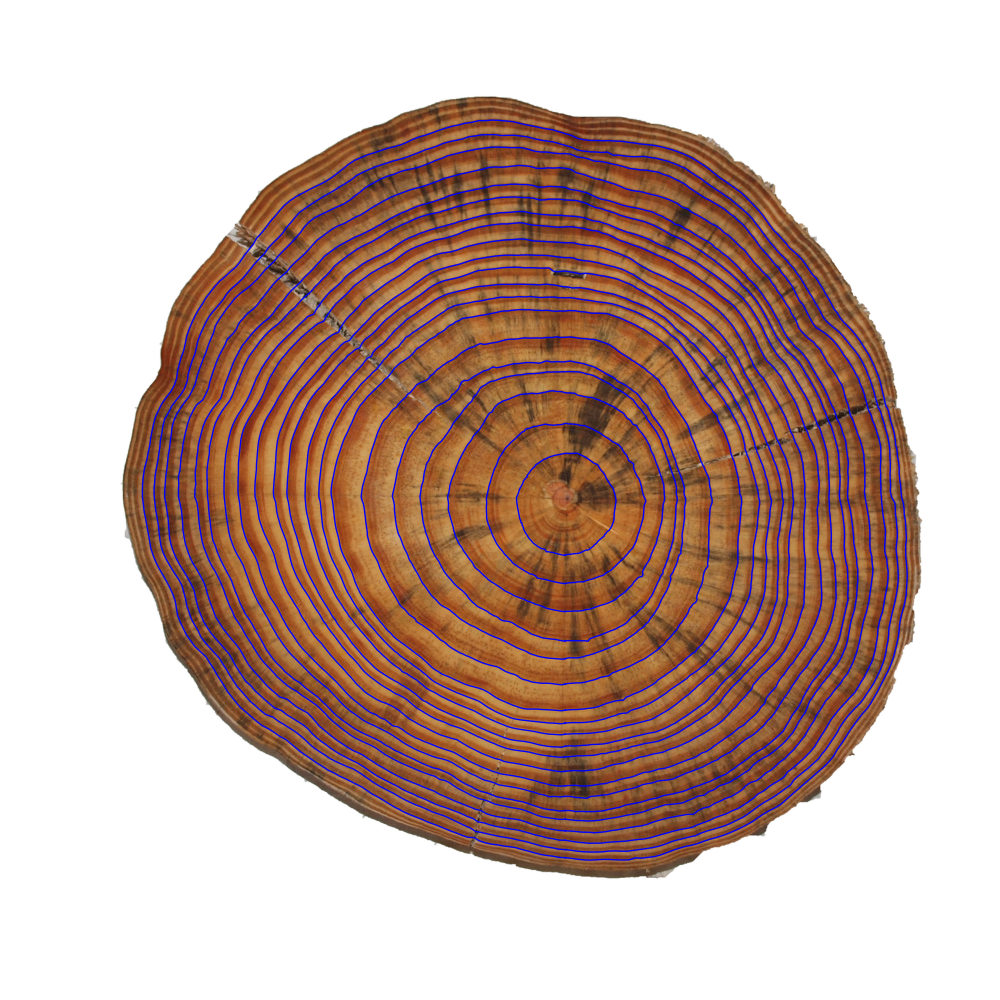
(a) F02a

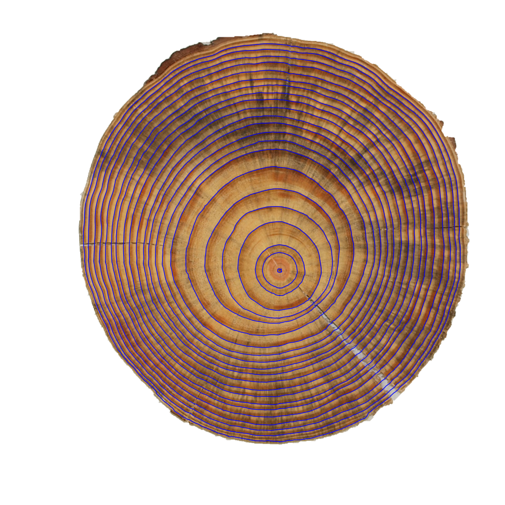
(b) F02b

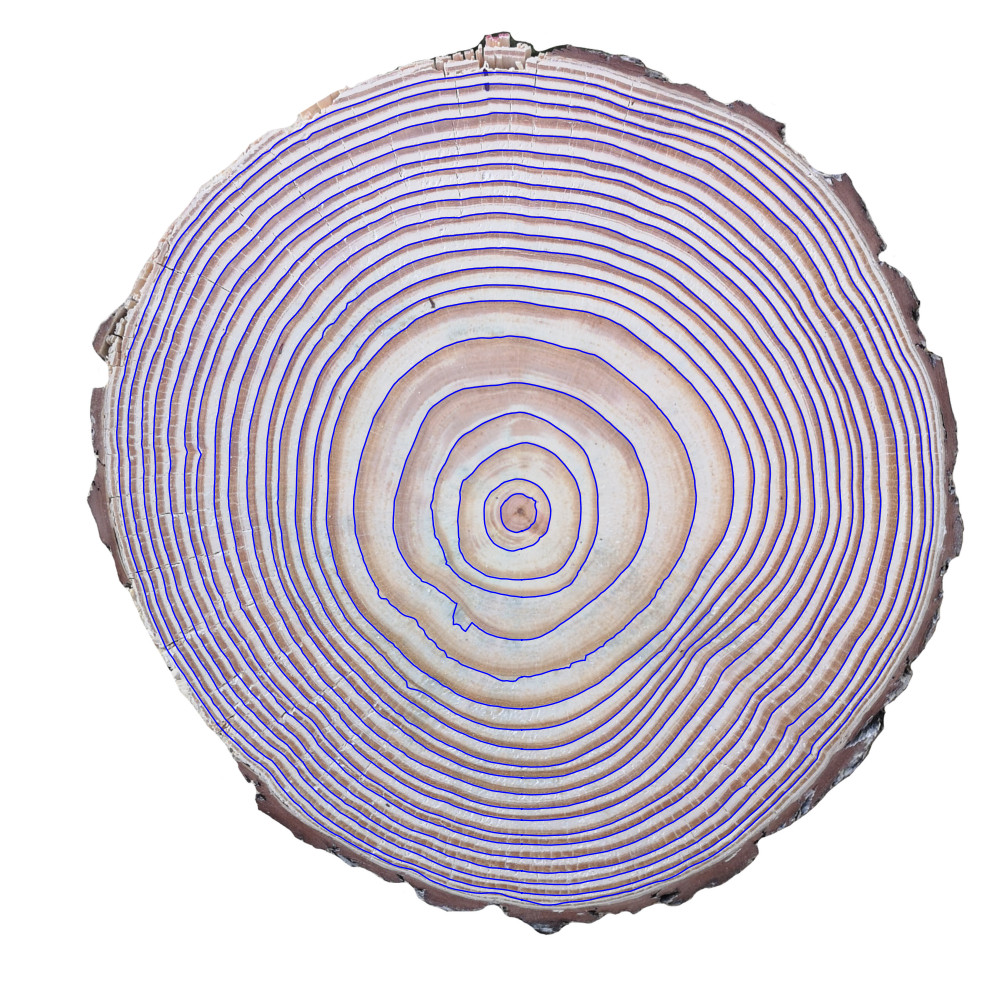
(c) F02c

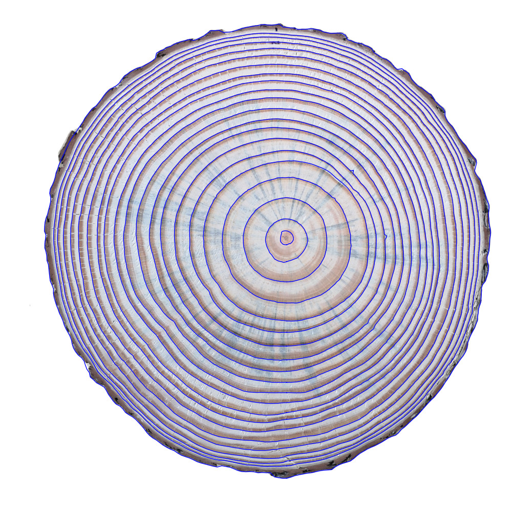
(d) F02d

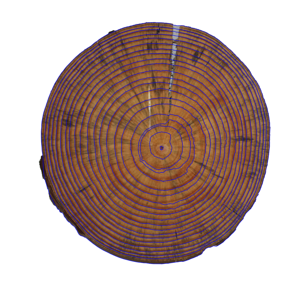
(e) F02e

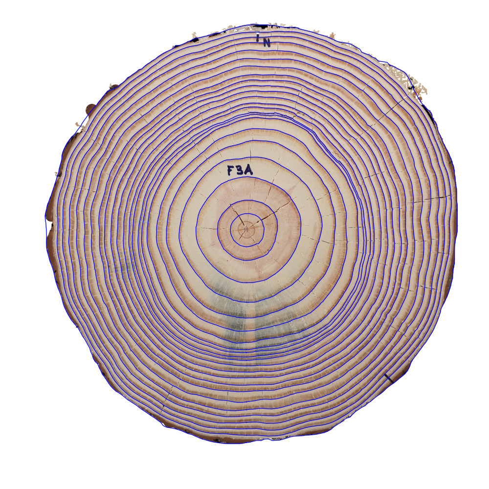
(f) F03c

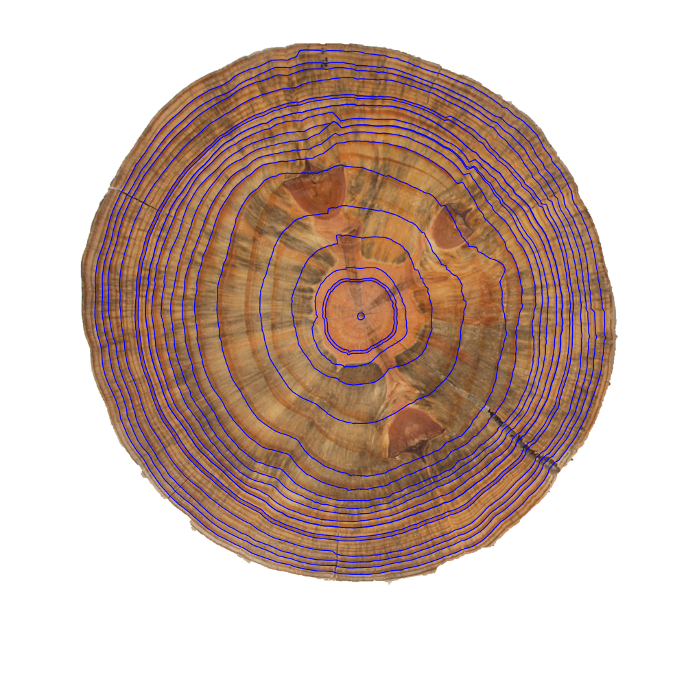
(g) F07b

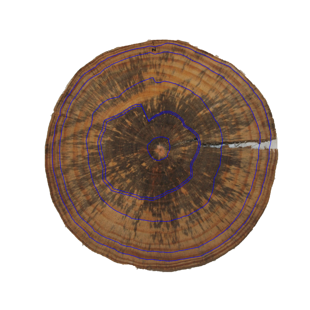
(h) L02b

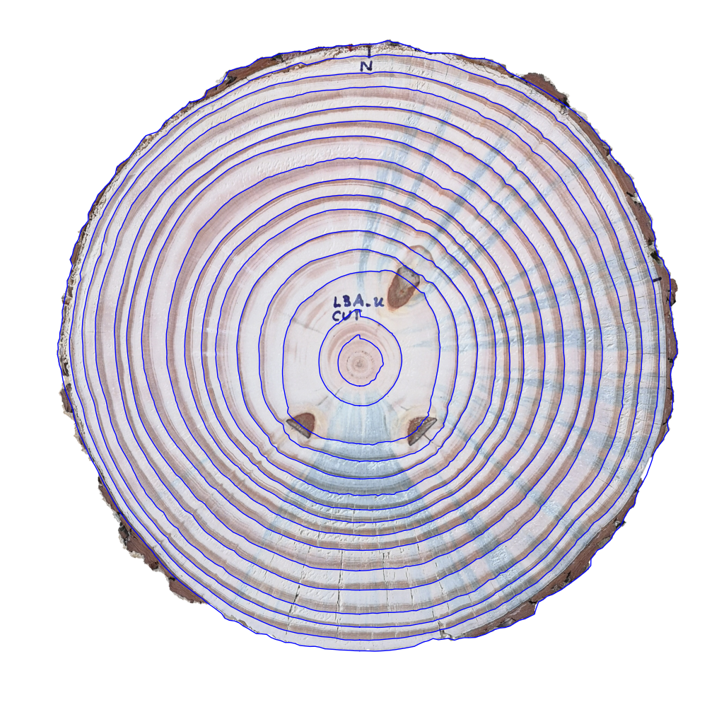
(i) L03c

Figure 25: Some results for the UruDendro dataset.

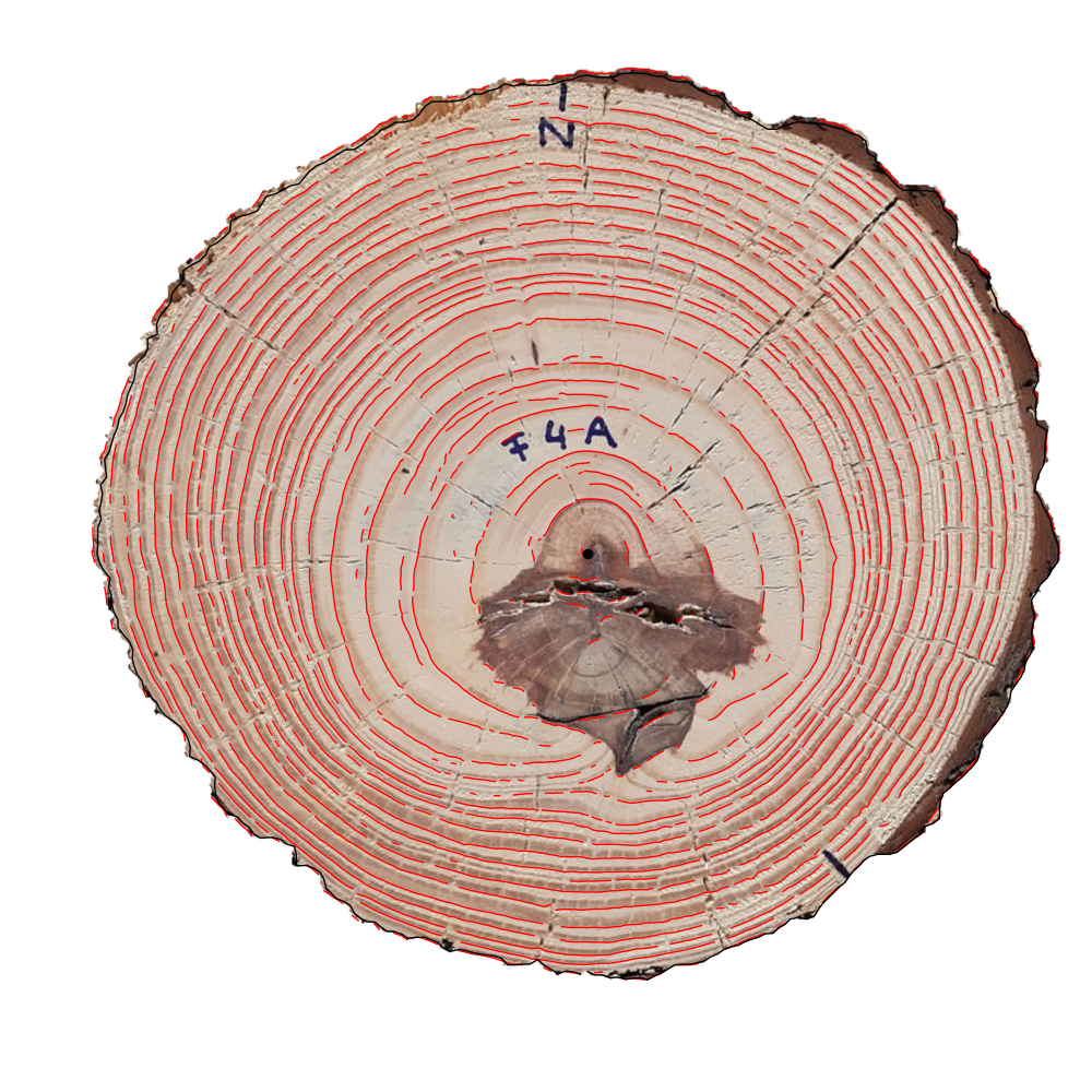
(a) Chains

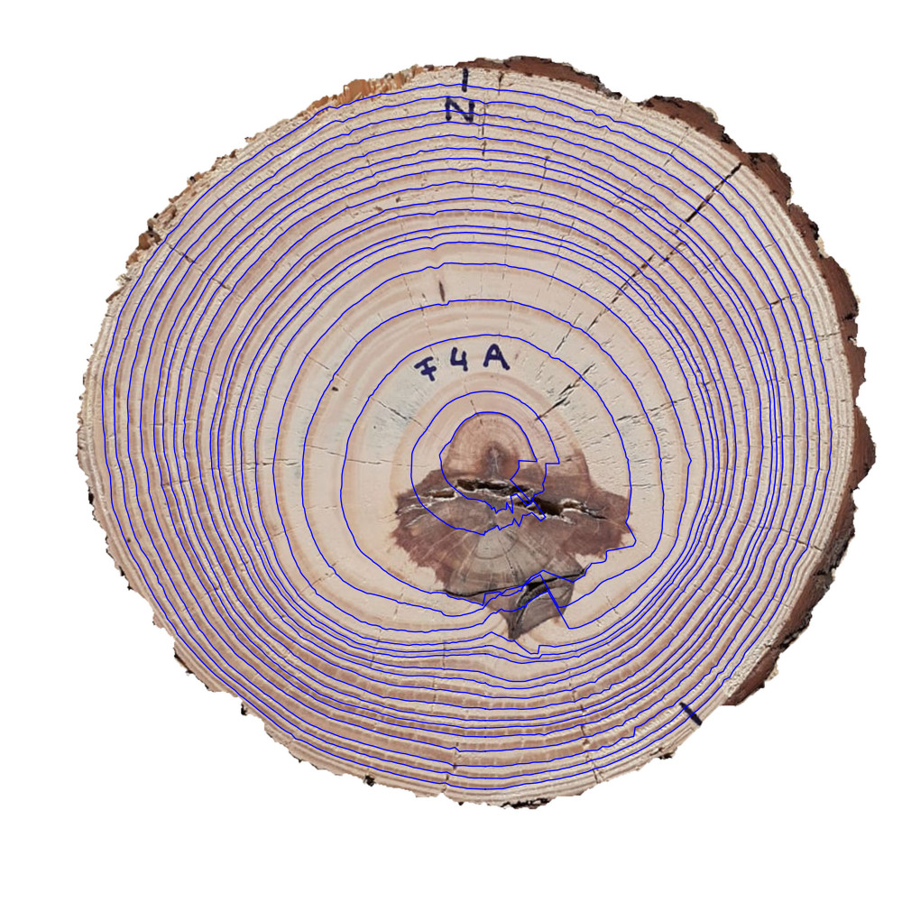
(b) Output

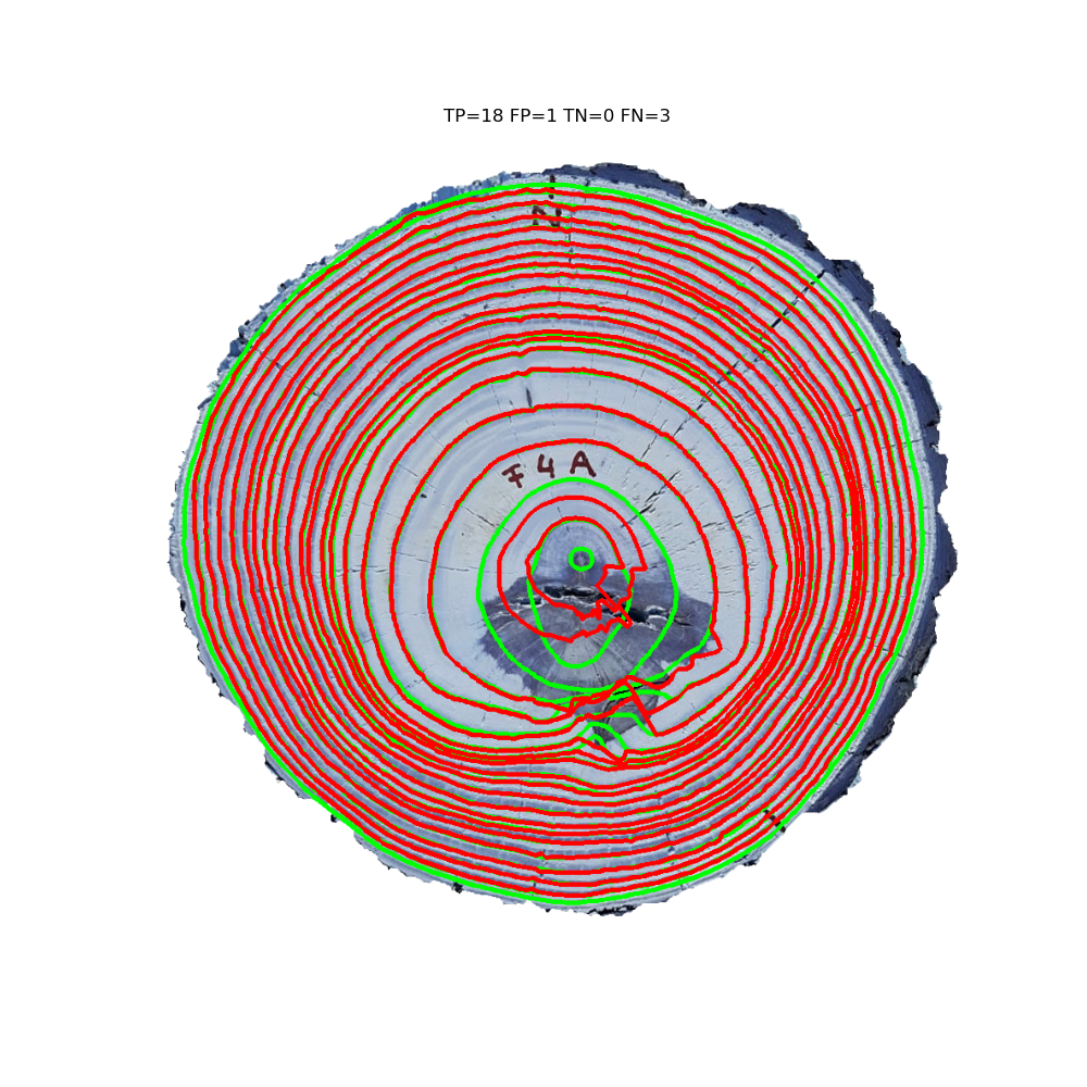
(c) Gt and Dt

Figure 26: Method result for disk F04c. Note how the knot stain perturbs the edge detection step.

Figure 27 illustrates our method results for disk L09e. Despite the presence of two important cracks and some fungus stains, the method successfully detects 13/15 rings, which means an F1-Score of 93%.

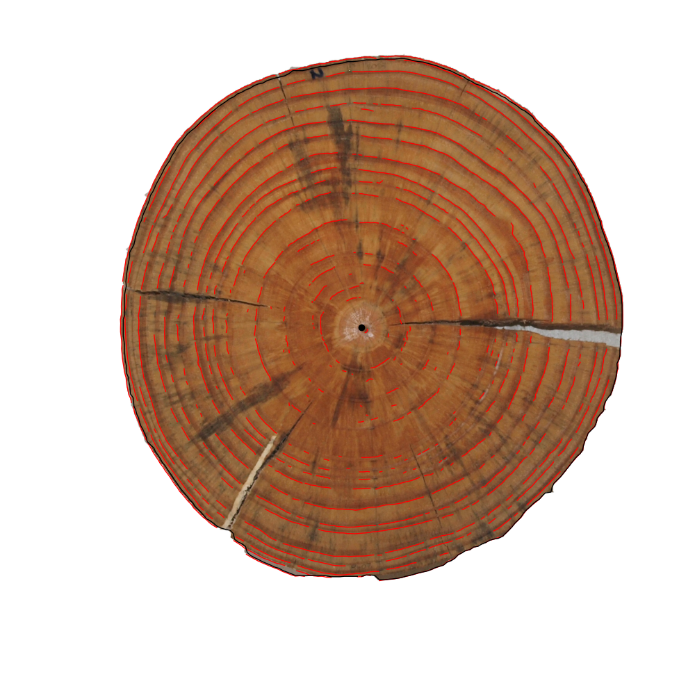
(a) Chains

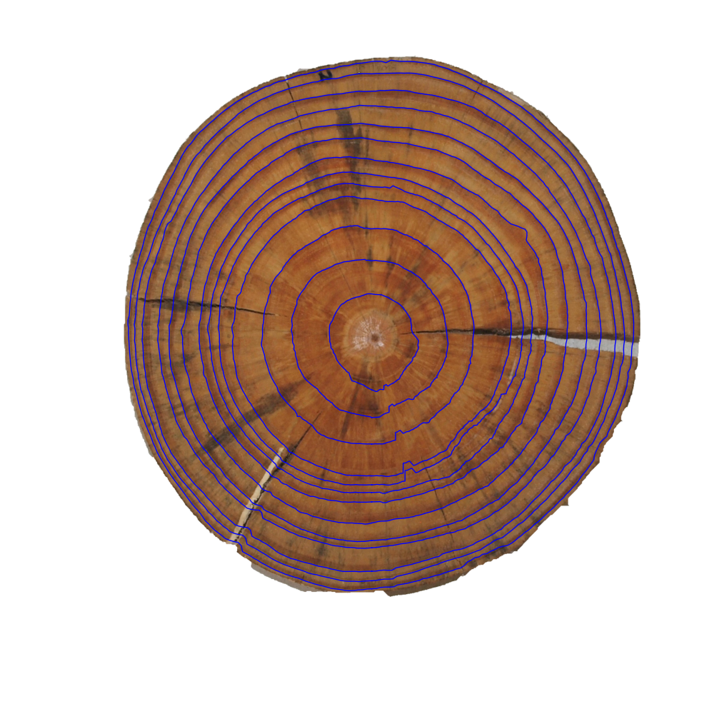
(b) Output

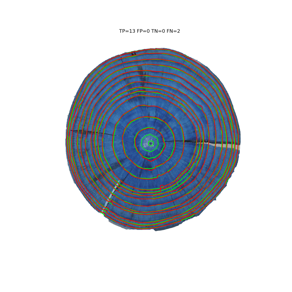
(c) Gt and Dt

Figure 27: Method result for disk L09e. Note how the method succeeds in detecting almost all the rings (FN=2 and FP=0) despite the cracks and fungus stain

As seen in Table 7, the CS-TRD algorithm generally works fine even if for some images it has problems. Let’s discuss some examples, such as images L02b, F07e, and L02d.

Figure 28 illustrates the results for disk L02b. Figure 28(c), shows the detected rings in red and the ground truth in green. Four detections are closed curves and determined as correct (TP), while two are determined as incorrect (FP). Counting from the center to the border, the first detection is correct, and the next two are bad, corresponding to the second and third rings. Analyzing the chains step output shown in Figure 28(a), it seems clear that there is not enough edge information to see the rings due to the fungus stain.

A similar situation happens for disk F07e, Figure 29. There is a strong fungus stain presence which makes that some rings do not have enough edges to form a closed curve.

The method results are slightly better for disk L02d with an F-Score of 58% in the presence of the same fungus stain issue that former disks. Figure 30(a) illustrates this case and how the fungus perturbs the edge detection step in the middle of the disk.

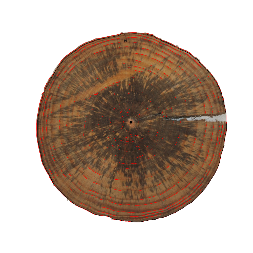
(a) Chains

(b) Output

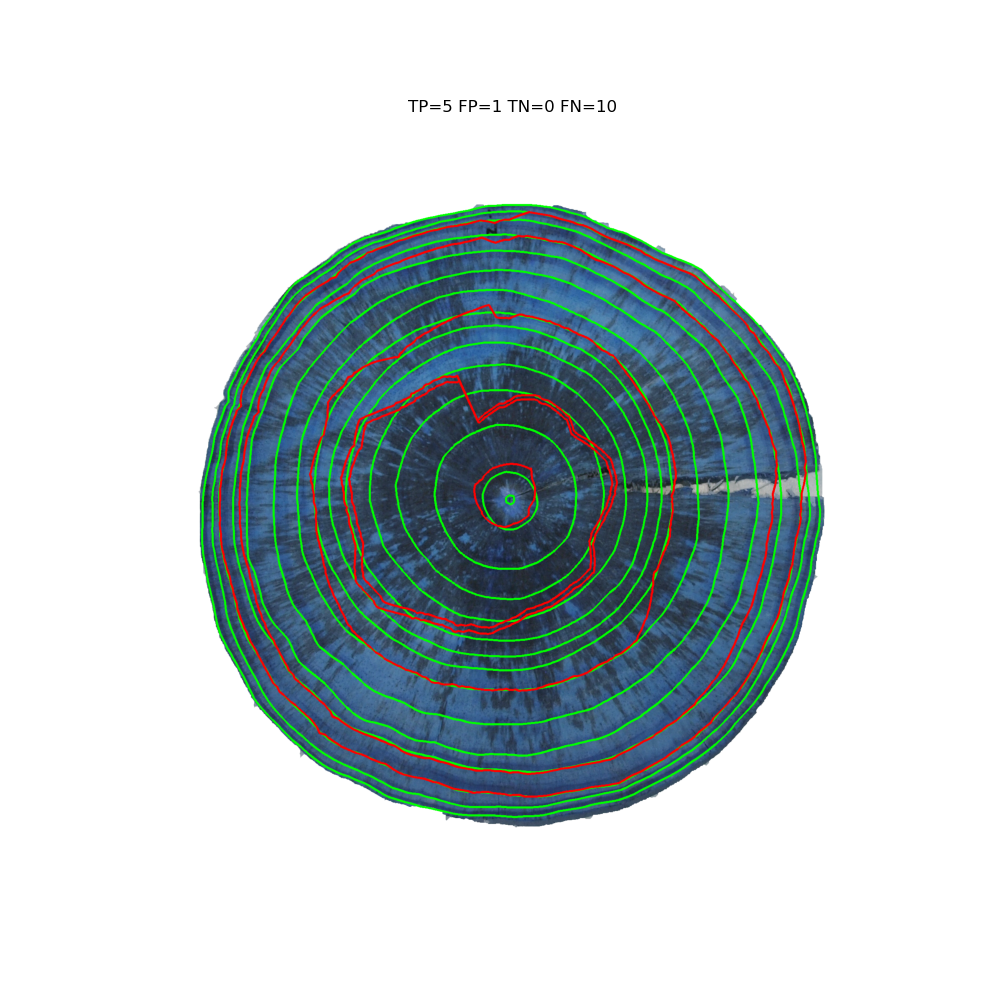
(c) Gt and Dt

Figure 28: Method result for disk L02b. Note how the fungus stain perturbs the edge detection step.

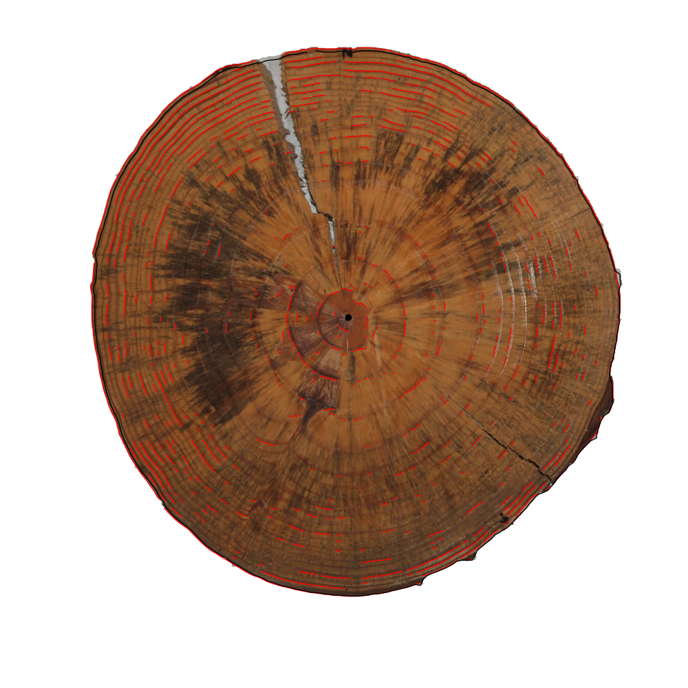
(a) Chains

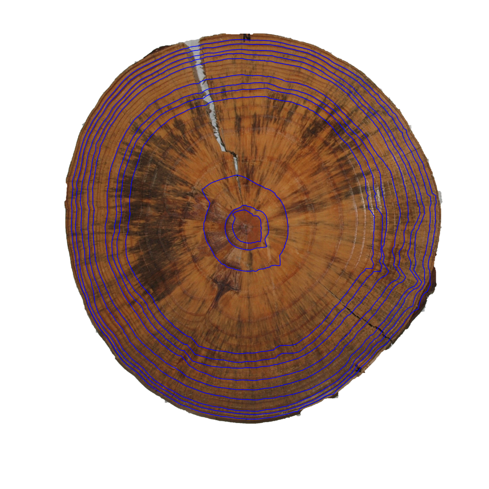
(b) Output

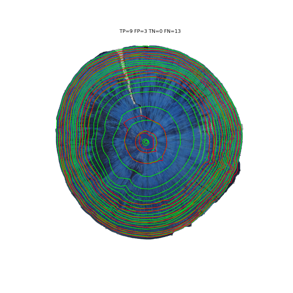
(c) Gt and Dt

Figure 29: Method result for disk F07e. Note how the fungus stain perturbs the edge detection step.

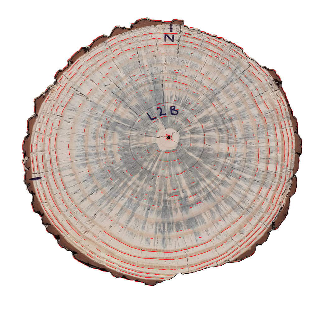
(a) Chains

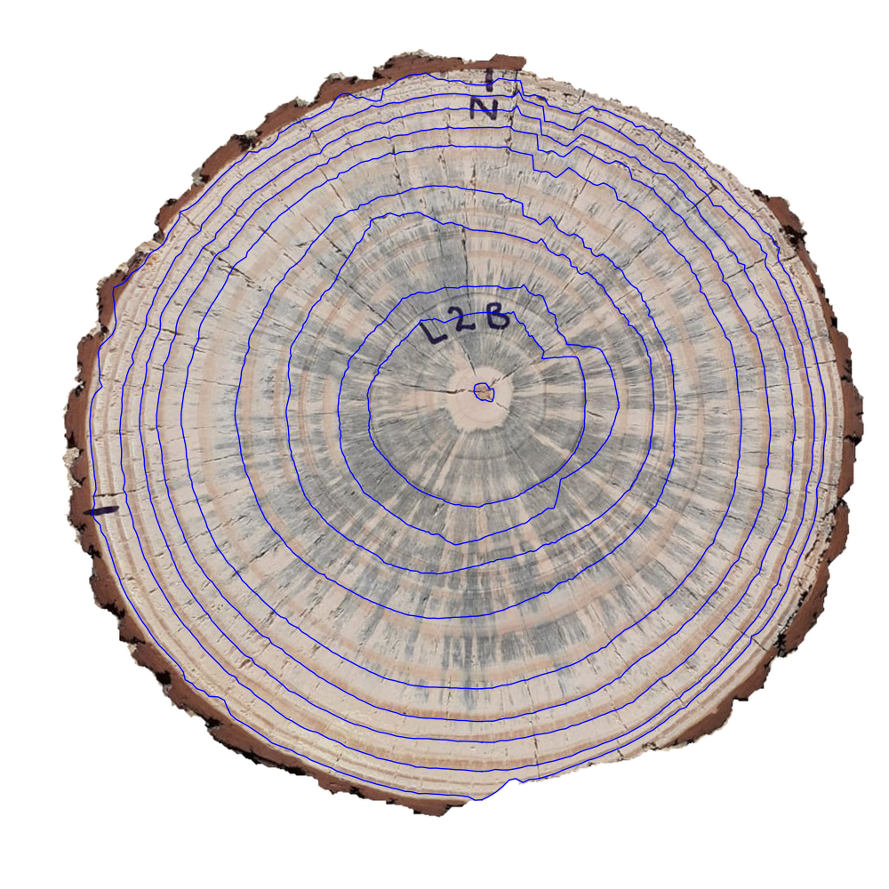
(b) Output

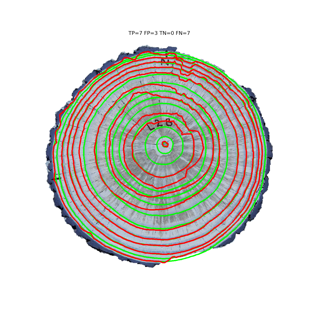
(c) Gt and Dt

Figure 30: Method result for disk L02d. Note how the fungus stain perturbs the edge detection step.

7 Conclusions and future work

An automatic method (besides the pith detection, for which an automatic algorithm exists [4]) for Tree Ring Detection of cross-section wood images is presented, which achieves an F-Score of 97% in the Kennel dataset and an F-Score of 89% in the (more difficult) UruDendro dataset.

The method executes at an average execution time of 17 seconds in the UruDendro dataset and 11 seconds in Kennel dataset. Compared with the time that each annotator needed to delineate every disk manually, 3 hours on average, is a vast improvement. CS-TRD method can be fully implemented in C++ to accelerate the execution time compared to a Python implementation. This will allow using the method in real-time applications.

In the future, we will include the automatic detection of the pith, extend the method to other tree species and explore machine-learning techniques to learn the pattern in the data.

Image Credits

Images from the UruDendro dataset.
Images taken from a [8]
original images from the Kennel dataset.

References

- [1] Mauricio Cerda, Nancy Hitschfeld-Kahler, and Domingo Mery, Robust tree-ring detection, in Advances in Image and Video Technology, Second Pacific Rim Symposium, PSIVT 2007, Santiago, Chile, December 17-19, 2007, Proceedings, Domingo Mery and Luis Rueda, eds., vol. 4872 of Lecture Notes in Computer Science, Springer, 2007, pp. 575–585.
- [2] Alex Clark, Pillow (pil fork) documentation, 2015.
- [3] Brook M. Constantz, Andrew A. Port, and Randall S. Senock, Comparing automatically generated and manually measured tree-ring transects of growth trends with hawaiian sandalwood as an example species, Dendrochronologia, 68 (2021), p. 125831.
- [4] Rémi Decelle, Phuc Ngo, Isabelle Debled-Rennesson, Frédéric Mothe, and Fleur Longuetaud, Ant Colony Optimization for Estimating Pith Position on Images of Tree Log Ends, Image Processing On Line, 12 (2022), pp. 558–581. https://doi.org/10.5201/ipol.2022.338.
- [5] Frédéric Devernay, A non-maxima suppression method for edge detection with sub-pixel accuracy, tech. report, INRIA RESEARCH REP. 2724, SOPHIAANTIPOLIS, 1995.
- [6] Philipp Duncker, Detection and Grading of Compression Wood, 11 2014, pp. 201–224.
- [7] Anna Fabijańska and Małgorzata Danek, Deepdendro – a tree rings detector based on a deep convolutional neural network, Computers and Electronics in Agriculture, 150 (2018), pp. 353–363.
- [8] Anna Fabijańska, Małgorzata Danek, Joanna Barniak, and Adam Piórkowski, Towards automatic tree rings detection in images of scanned wood samples, Computers and Electronics in Agriculture, 140 (2017), pp. 279–289.
- [9] Alexander Gillert, Giulia Resente, Alba Anadon-Rosell, Martin Wilmking, and Uwe Freiherr von Lukas, Iterative next boundary detection for instance segmentation of tree rings in microscopy images of shrub cross sections, 2022.
- [10] Rafael Grompone von Gioi and Gregory Randall, A Sub-Pixel Edge Detector: an Implementation of the Canny/Devernay Algorithm, Image Processing On Line, 7 (2017), pp. 347–372. https://doi.org/10.5201/ipol.2017.216.
- [11] Michael Henke and Branislav Sloboda, Semiautomatic tree ring segmentation using active contours and an optimised gradient operator, Forestry Journal, 60 (2014), pp. 185 – 190.
- [12] Itseez, Open source computer vision library. https://github.com/itseez/opencv, 2015.
- [13] Pol Kennel, Philippe Borianne, and Gérard Subsol, An automated method for tree-ring delineation based on active contours guided by DT-CWT complex coefficients in photographic images: Application to abies alba wood slice images, Comput. Electron. Agric., 118 (2015), pp. 204–214.
- [14] Nick G. Kingsbury, Complex wavelets for shift invariant analysis and filtering of signals, Applied and Computational Harmonic Analysis, 10 (2001), pp. 234–253.
- [15] Kayla Makela, Tim Ophelders, Michelle Quigley, Elizabeth Munch, Daniel Chitwood, and Asia Dowtin, Automatic tree ring detection using jacobi sets, 2020.
- [16] Henry Marichal, Diego Passarella, Christine Lucas, Ludmila Profumo, Veronica Casaravilla, Maria Noel Rocha Galli, Serrana Ambite, and Gregory Randall, UruDendro: An Uruguayan Disk Wood Database For Image Processing. https://iie.fing.edu.uy/proyectos/madera.
- [17] R. Stockton Maxwell and Lars-Åke Larsson, Measuring tree-ring widths using the coorecorder software application, Dendrochronologia, 67 (2021), p. 125841.
- [18] Kristin Norell, An automatic method for counting annual rings in noisy sawmill images, in Image Analysis and Processing – ICIAP 2009, Pasquale Foggia, Carlo Sansone, and Mario Vento, eds., Berlin, Heidelberg, 2009, Springer Berlin Heidelberg, pp. 307–316.
- [19] Kristin Norell, Joakim Lindblad, and Stina Svensson, Grey weighted polar distance transform for outlining circular and approximately circular objects, 14th International Conference on Image Analysis and Processing (ICIAP 2007), (2007), pp. 647–652.
- [20] Miroslav Poláek, Alexis H. Arizpe, Patrick Hüther, Lisa Weidlich, Sonja Steindl, and Kelly L. Swarts, Automation of tree-ring detection and measurements using deep learning, bioRxiv, (2022).
- [21] Xuebin Qin, Zichen Zhang, Chenyang Huang, Masood Dehghan, Osmar R. Zaïane, and Martin Jägersand, U-net: Going deeper with nested u-structure for salient object detection, CoRR, abs/2005.09007 (2020).
- [22] Jingning Shi, Wei Xiang, Qijing Liu, and Sher Shah, Mtreering: An r package with graphical user interface for automatic measurement of tree ring widths using image processing techniques, Dendrochronologia, 58 (2019), p. 125644.
- [23] Kentaro Wada, Labelme: Image Polygonal Annotation with Python.
- [24] Hong Zhou, Rong Feng, Hua hong Huang, Er pei Lin, and Jun lin Yu, Method of tree-ring image analysis for dendrochronology, Optical Engineering, 51 (2012), p. 077202.
- [25] Karel Zuiderveld, Contrast Limited Adaptive Histogram Equalization, Academic Press Professional, Inc., USA, 1994, p. 474–485.