Adaptive choice of near-optimal expansion points for interpolation-based structure-preserving model reduction

Abstract

Interpolation-based methods are well-established and effective approaches for the efficient generation of accurate reduced-order surrogate models. Common challenges for such methods are the automatic selection of good or even optimal interpolation points and the appropriate size of the reduced-order model. An approach that addresses the first problem for linear, unstructured systems is the Iterative Rational Krylov Algorithm (IRKA), which computes optimal interpolation points through iterative updates by solving linear eigenvalue problems. However, in the case of preserving internal system structures, optimal interpolation points are unknown, and heuristics based on nonlinear eigenvalue problems result in numbers of potential interpolation points that typically exceed the reasonable size of reduced-order systems. In our work, we propose a projection-based iterative interpolation method inspired by IRKA for generally structured systems to adaptively compute near-optimal interpolation points as well as an appropriate size for the reduced-order system. Additionally, the iterative updates of the interpolation points can be chosen such that the reduced-order model provides an accurate approximation in specified frequency ranges of interest. For such applications, our new approach outperforms the established methods in terms of accuracy and computational effort. We show this in numerical examples with different structures.

We propose a new algorithm for the construction of interpolating, structured, reduced-order models via projection. The method efficiently determines new interpolation points from the solutions of low-dimensional linear eigenvalue problems, adaptively chooses an appropriate size of the reduced-order model, and can be used to obtain high-fidelity approximations in limited frequency ranges of interest.

1 Introduction

Simulation, control and optimization of dynamical systems are essential for many applications. In this work, we consider structured linear systems in the frequency (Laplace) domain of the form

$$\Sigma\colon\begin{cases}\boldsymbol{\mathcal{K}}(s)\boldsymbol{X}(s)=\boldsymbol{\mathcal{B}}(s)\boldsymbol{U}(s),\quad\boldsymbol{Y}(s)=\boldsymbol{\mathcal{C}}(s)\boldsymbol{X}(s),\end{cases}$$ (1)

where $\boldsymbol{\mathcal{K}}\colon\mathbb{C}\to\mathbb{C}^{n\times n}$ describes the system dynamics, $\boldsymbol{\mathcal{B}}\colon\mathbb{C}\to\mathbb{C}^{n\times m}$ the system’s input and $\boldsymbol{\mathcal{C}}\colon\mathbb{C}\to\mathbb{C}^{p\times n}$ the system’s output behavior; see [10] for motivation of Eq. 1 example systems. The functions $\boldsymbol{X}\colon\mathbb{C}\to\mathbb{C}^{n}$, $\boldsymbol{U}\colon\mathbb{C}\to\mathbb{C}^{m}$ and $\boldsymbol{Y}\colon\mathbb{C}\to\mathbb{C}^{p}$ denote the internal states, inputs and outputs, respectively. For all $s\in\mathbb{C}$ for which $\boldsymbol{\mathcal{K}}$ is invertible, and $\boldsymbol{\mathcal{B}}$ and $\boldsymbol{\mathcal{C}}$ can be evaluated, the corresponding transfer function $\boldsymbol{H}\colon\mathbb{C}\to\mathbb{C}^{p\times m}$ directly relates the system’s inputs to outputs:

$$\boldsymbol{H}(s)=\boldsymbol{\mathcal{C}}(s)\boldsymbol{\mathcal{K}}(s)^{-1}\boldsymbol{\mathcal{B}}(s).$$ (2)

The most commonly considered structure of dynamical systems is given by first-order differential equations in the time domain

$$\Sigma\colon\begin{cases}\boldsymbol{E}\dot{\boldsymbol{x}}(t)=\boldsymbol{A}\boldsymbol{x}(t)+\boldsymbol{B}\boldsymbol{u}(t),\quad\boldsymbol{y}(t)=\boldsymbol{C}\boldsymbol{x}(t),\end{cases}$$ (3)

with the system matrices $\boldsymbol{A},\boldsymbol{E}\in\mathbb{R}^{n\times n}$, $\boldsymbol{B}\in\mathbb{R}^{n\times m}$ and $\boldsymbol{C}\in\mathbb{R}^{p\times n}$. Systems of the form Eq. 3 are also commonly referred to as unstructured systems due to them being considered as the standard case. Applying the Laplace transformation to Eq. 3 yields a frequency-dependent system of the form Eq. 1, with

$$\boldsymbol{\mathcal{K}}(s)=(s\boldsymbol{E}-\boldsymbol{A})^{-1},\quad\boldsymbol{\mathcal{B}}(s)=\boldsymbol{B},\quad\boldsymbol{\mathcal{C}}(s)=\boldsymbol{C},$$

and the corresponding transfer function $\boldsymbol{H}(s)=\boldsymbol{C}(s\boldsymbol{E}-\boldsymbol{A})^{-1}\boldsymbol{B}$. On the other hand, the modeling of specific physical phenomena hands down other differential structures into dynamical systems. The modeling of mechanical structures, structural vibrations, wave movement or electrical circuits classically leads to differential equations with second-order time derivatives, which in frequency domain are described by transfer functions of the form

$$\boldsymbol{H}(s)=(\boldsymbol{C}_{\mathrm{p}}+s\boldsymbol{C}_{\mathrm{v}})(s^{2}\boldsymbol{M}+s\boldsymbol{D}+\boldsymbol{K})^{-1}\boldsymbol{B};$$ (4)

see, for example, [1, 49, 51] and references therein. A different structure occurs when modeling incomplete systems resulting in time-delay structures, which are expressed as exponential terms in the frequency domain, e.g., with the transfer function

$$\boldsymbol{H}(s)=\boldsymbol{C}(s\boldsymbol{E}-\boldsymbol{A}_{\mathrm{0}}-\operatorname{e}^{-\tau s}\boldsymbol{A}_{\mathrm{d}})^{-1}\boldsymbol{B},$$ (5)

for some constant time delay $\tau>0$; see, e.g., [27]. Many other structures exist in literature, which are used to model, for example, poroelasticity [5], viscoelasticity [47], or interior acoustic problems [21]. While some structures, like second-order systems Eq. 4, can be reformulated into standard form Eq. 3, this is not necessarily possible for all occurring structures, including time-delay systems Eq. 5. Also, by reformulation into unstructured form, the number of states increases and structure inherent properties are typically lost in subsequent computational procedures.

In general, there is a demand for highly accurate models in practical applications. As a result, the number of equations describing Eq. 1 vastly grows and the computational efficient solution of Eq. 1 in terms of resources such as time and memory is often impossible. Model order reduction methods are a remedy to this problem as they aim for the construction of cheap-to-evaluate yet accurate surrogate models that approximate the systems’ input-to-output behavior while being described by a significantly smaller number of equations $r\ll n$, which eases the demand on computational resources required for the evaluation of the systems. Many model reduction techniques have been developed for unstructured systems Eq. 3; see, for example, [3]. In addition, the preservation of internal system structures such as Eqs. 4 and 5 is desired as this typically yields more accurate approximations as well as the preservation of structure inherent properties. Also, if the reduced-order model is to be coupled to other systems, preserving the structure is advantageous because the same coupling conditions as for the full-order model can be applied to the reduced surrogate [22].

Several structure-preserving model order reduction methods have been developed in recent years. Many of these have been tailored to particular structures that occur, for example, in vibrational problems [34, 9, 12, 49], network systems [20, 24], or systems with Hamiltonian structure [13, 31, 33]. The framework in [10] allows the reduction of dynamical systems with arbitrary internal structures based on transfer function interpolation. The quality of reduced-order models obtained by interpolation strongly depends on the choice of interpolation points. Therefore, a variety of strategies has been developed to perform successive greedy searches for suitable interpolation points based on estimating the approximation error [19, 17, 25, 42, 41, 7, 26] or computing the exact error in, for example, the $\mathcal{L}_{\infty}$-norm [2, 45].

On the other hand, the Iterative Rational Krylov Algorithm (IRKA) is a well established interpolation method for unstructured systems Eq. 3 that iteratively updates the interpolation points [29]. At convergence, the interpolating reduced-order model satisfies the necessary $\mathcal{H}_{2}$-optimality conditions. Several extensions of IRKA for structured systems using similar ideas have been proposed. For second-order systems Eq. 4, the SO-IRKA method from [52] aims for an iterative process similar to IRKA. In [6], this has been considered as basis for a method to choose the resulting approximation order adaptively. Transfer Function IRKA (TF-IRKA) [11] can be applied to arbitrarily structured systems and yields $\mathcal{H}_{2}$-optimal but unstructured reduced-order models. A structure-preserving variant of TF-IRKA has been proposed in [46].

A different take on structured model order reduction are data-driven methods. Since here only measurements of the transfer function Eq. 2 are used to compute realizations of dynamical systems, the original structure can be arbitrary. One of the most well-known approaches of this type is the Loewner framework, which constructs a reduced-order model that interpolates provided data samples [39]. The original formulation of the Loewner framework only considers the construction of unstructured systems Eq. 3, but it has been extended to find structured realizations in [44]. Recently, structured extensions of the barycentric form for second-order systems Eq. 4 have been proposed that allow the extension of further data-driven frequency domain methods to the structure-preserving setting [28, 50].

In this work, we present a new approach to compute accurate reduced-order models that preserve the internal structure of the original system. Based on an IRKA-like iteration scheme, the new method computes in every step a new set of interpolation points (and tangential directions) which are then employed in the structure-preserving interpolation framework [10]. Instead of considering nonlinear eigenvalue problems corresponding to the resolvent terms of the structured systems, the Loewner framework allows us to solve instead linear eigenvalue problems in each step and to determine the approximation order adaptively and with respect to limited frequency regions of interest if desired.

The remainder of this manuscript is structured as follows: After introducing the mathematical preliminaries in Section 2, we revisit the structure-preserving transfer function IRKA and extend that method to the case of multiple-input/multiple-output systems in Section 3.1. Our new model reduction method is then described in Section 3.2. In Section 4, a number of numerical experiments are used to compare the new method to established model reduction techniques. The paper is concluded in Section 5.

2 Mathematical preliminaries

2.1 Structure-preserving interpolation via projection

We consider here interpolation-based model order reduction methods, which compute surrogate models approximating the dynamics of the high-fidelity system Eq. 1 while having much smaller dimensions $r\ll n$. Structure-preserving model order reduction methods construct approximations of Eq. 1 with the same internal structure

$$\hstretch{2.5}{\hat{\hstretch{.4}{\Sigma}}}\colon\begin{cases}\hstretch{2.5}{\hat{\hstretch{.4}{\boldsymbol{\mathcal{K}}}}}(s){\hstretch{2.5}{\hat{\hstretch{.4}{\boldsymbol{X}\mkern 3.0mu}}}\mkern-3.0mu}{}(s)={\hstretch{2.5}{\hat{\hstretch{.4}{\boldsymbol{\mathcal{B}}\mkern 1.0mu}}}\mkern-1.0mu}{}(s)\boldsymbol{U}(s),\quad\hstretch{2.5}{\hat{\hstretch{.4}{\boldsymbol{Y}}}}(s)={\hstretch{2.5}{\hat{\hstretch{.4}{\boldsymbol{\mathcal{C}}\mkern 2.0mu}}}\mkern-2.0mu}{}(s){\hstretch{2.5}{\hat{\hstretch{.4}{\boldsymbol{X}\mkern 3.0mu}}}\mkern-3.0mu}{}(s),\end{cases}$$ (6)

where $\hstretch{2.5}{\hat{\hstretch{.4}{\boldsymbol{\mathcal{K}}}}}\colon\mathbb{C}\to\mathbb{C}^{r\times r}$, ${\hstretch{2.5}{\hat{\hstretch{.4}{\boldsymbol{\mathcal{B}}\mkern 1.0mu}}}\mkern-1.0mu}{}\colon\mathbb{C}\to\mathbb{C}^{r\times m}$, ${\hstretch{2.5}{\hat{\hstretch{.4}{\boldsymbol{\mathcal{C}}\mkern 2.0mu}}}\mkern-2.0mu}{}\colon\mathbb{C}\to\mathbb{C}^{p\times r}$ and ${\hstretch{2.5}{\hat{\hstretch{.4}{\boldsymbol{X}\mkern 3.0mu}}}\mkern-3.0mu}{}\colon\mathbb{C}\to\mathbb{C}^{r}$, $\hstretch{2.5}{\hat{\hstretch{.4}{\boldsymbol{Y}}}}\colon\mathbb{C}\to\mathbb{C}^{p}$. Additionally, the compositions of the matrix-valued functions in Eqs. 1 and 6 are the same: If the center term in Eq. 1 is given in frequency-affine form

$$\boldsymbol{\mathcal{K}}(s)=\sum\limits_{j=1}^{n_{\boldsymbol{\mathcal{K}}}}g_{j}(s)\boldsymbol{\mathcal{K}}_{j},$$ (7)

with $g_{j}\colon\mathbb{C}\to\mathbb{C}$ and constant matrices $\boldsymbol{\mathcal{K}}_{j}\in\mathbb{C}^{n\times n}$, for $j=1,\ldots,n_{\boldsymbol{\mathcal{K}}}$, then the center term of the reduced-order model must have the form

$$\hstretch{2.5}{\hat{\hstretch{.4}{\boldsymbol{\mathcal{K}}}}}(s)=\sum\limits_{j=1}^{n_{\boldsymbol{\mathcal{K}}}}g_{j}(s)\hstretch{2.5}{\hat{\hstretch{.4}{\boldsymbol{\mathcal{K}}}}}_{j},$$ (8)

where $\hstretch{2.5}{\hat{\hstretch{.4}{\boldsymbol{\mathcal{K}}}}}_{j}\in\mathbb{C}^{r\times r}$, for $j=1,\ldots,n_{\boldsymbol{\mathcal{K}}}$. Since the scalar functions in Eqs. 7 and 8 are identical, the internal system structure is preserved and the system matrices $\boldsymbol{\mathcal{K}}_{j}$ of the full-order system can be replaced by their reduced-order counterparts $\hstretch{2.5}{\hat{\hstretch{.4}{\boldsymbol{\mathcal{K}}}}}_{j}$. The same relations must hold for the input and output terms $\boldsymbol{\mathcal{B}}$ and $\boldsymbol{\mathcal{C}}$. Consider as an example the second-order system with transfer function Eq. 4 from Section 1. A structure-preserving reduced-order model will be of the form

$${\hstretch{2.5}{\hat{\hstretch{.4}{\boldsymbol{H}\mkern 4.0mu}}}\mkern-4.0mu}{}(s)=({\hstretch{2.5}{\hat{\hstretch{.4}{\boldsymbol{C}\mkern 2.0mu}}}\mkern-2.0mu}{}_{\mathrm{p}}+s{\hstretch{2.5}{\hat{\hstretch{.4}{\boldsymbol{C}\mkern 2.0mu}}}\mkern-2.0mu}{}_{\mathrm{v}})(s^{2}{\hstretch{2.5}{\hat{\hstretch{.4}{\boldsymbol{M}\mkern 3.0mu}}}\mkern-3.0mu}{}+s{\hstretch{2.5}{\hat{\hstretch{.4}{\boldsymbol{D}\mkern 2.0mu}}}\mkern-2.0mu}{}+{\hstretch{2.5}{\hat{\hstretch{.4}{\boldsymbol{K}\mkern 3.0mu}}}\mkern-3.0mu}{})^{-1}{\hstretch{2.5}{\hat{\hstretch{.4}{\boldsymbol{B}\mkern 2.0mu}}}\mkern-2.0mu}{}.$$

To act as suitable surrogate, the reduced-order model must approximate the input-to-output behavior of the original system at least for a range of frequencies $s\in\mathbb{C}$, which are important for the application in question. In other words, the outputs of Eqs. 1 and 6 should match up to a specified tolerance $\tau$ in appropriate norms for a given input:

$$\lVert\boldsymbol{Y}-\hstretch{2.5}{\hat{\hstretch{.4}{\boldsymbol{Y}}}}\rVert\leq\tau\cdot\lVert\boldsymbol{U}\rVert.$$

For many time domain models and, in general, frequency domain models, the relation above can be reformulated in terms of the transfer functions of the original and reduced-order model such that

$$\lVert\boldsymbol{H}-{\hstretch{2.5}{\hat{\hstretch{.4}{\boldsymbol{H}\mkern 4.0mu}}}\mkern-4.0mu}{}\rVert\leq\tau$$

holds.

Following [10], any matrix-valued function of the form Eq. 2 can be interpolated by a reduced-order transfer function ${\hstretch{2.5}{\hat{\hstretch{.4}{\boldsymbol{H}\mkern 4.0mu}}}\mkern-4.0mu}{}$, while preserving the internal system structure using the projection approach. Given two reduction spaces with basis matrices $\boldsymbol{V},\boldsymbol{W}\in\mathbb{C}^{n\times r}$, the reduced-order model is computed by

$$\hstretch{2.5}{\hat{\hstretch{.4}{\boldsymbol{\mathcal{K}}}}}(s)=\boldsymbol{W}^{\mathsf{H}}\boldsymbol{\mathcal{K}}(s)\boldsymbol{V},\quad{\hstretch{2.5}{\hat{\hstretch{.4}{\boldsymbol{\mathcal{B}}\mkern 1.0mu}}}\mkern-1.0mu}{}(s)=\boldsymbol{W}^{\mathsf{H}}\boldsymbol{\mathcal{B}}(s),\quad{\hstretch{2.5}{\hat{\hstretch{.4}{\boldsymbol{\mathcal{C}}\mkern 2.0mu}}}\mkern-2.0mu}{}(s)=\boldsymbol{\mathcal{C}}(s)\boldsymbol{V}.$$ (9)

While there are many potential choices for the basis matrices $\boldsymbol{V}$ and $\boldsymbol{W}$, we concentrate here on transfer function interpolation, i.e., the matrices $\boldsymbol{V},\boldsymbol{W}$ are constructed such that the transfer function ${\hstretch{2.5}{\hat{\hstretch{.4}{\boldsymbol{H}\mkern 4.0mu}}}\mkern-4.0mu}{}$ corresponding to Eq. 9 interpolates the full-order transfer function Eq. 2 at chosen points. The following proposition gives a concise overview.

Proposition 1 (Structured interpolation [10, Thm. 1]).

Let $\boldsymbol{H}$ be the transfer function Eq. 2 of a linear system, described by Eq. 1, and ${\hstretch{2.5}{\hat{\hstretch{.4}{\boldsymbol{H}\mkern 4.0mu}}}\mkern-4.0mu}{}$ the reduced-order transfer function constructed via projection Eq. 9. Let the matrix functions $\boldsymbol{\mathcal{C}}$, $\boldsymbol{\mathcal{K}}^{-1}$, $\boldsymbol{\mathcal{B}}$ and $\hstretch{2.5}{\hat{\hstretch{.4}{\boldsymbol{\mathcal{K}}}}}^{-1}$ be analytic in the interpolation point $\sigma\in\mathbb{C}$. Then, the following statements hold.

1. If $\operatorname{span}\left(\boldsymbol{\mathcal{K}}(\sigma)^{-1}\boldsymbol{\mathcal{B}}(\sigma)\right)\subseteq\operatorname{span}(\boldsymbol{V})$ holds, then $\boldsymbol{H}(\sigma)={\hstretch{2.5}{\hat{\hstretch{.4}{\boldsymbol{H}\mkern 4.0mu}}}\mkern-4.0mu}{}(\sigma)$.

2. If $\operatorname{span}\left(\boldsymbol{\mathcal{K}}(\sigma)^{-\mathsf{H}}\boldsymbol{\mathcal{C}}(\sigma)^{\mathsf{H}}\right)\subseteq\operatorname{span}(\boldsymbol{W})$ holds, then $\boldsymbol{H}(\sigma)={\hstretch{2.5}{\hat{\hstretch{.4}{\boldsymbol{H}\mkern 4.0mu}}}\mkern-4.0mu}{}(\sigma)$.

3. If $\boldsymbol{V}$ and $\boldsymbol{W}$ are constructed as above, then additionally $\boldsymbol{H}{}^{\prime}(\sigma)={\hstretch{2.5}{\hat{\hstretch{.4}{\boldsymbol{H}\mkern 4.0mu}}}\mkern-4.0mu}{}{}^{\prime}(\sigma)$ holds.

Overall, only linear systems of equations need to be solved for the construction of the basis matrices $\boldsymbol{V}$ and $\boldsymbol{W}$ in Proposition 1. However, the interpolation point $\sigma$ has to be known beforehand and its choice has a large influence on the approximation quality of the resulting reduced-order model. Traditionally, points are chosen linearly or logarithmically equidistant on the frequency axis $\mathfrak{i}\mathbb{R}$ in frequency ranges of interest to reduce the worst case approximation error of the transfer function given by the $\mathcal{L}_{\infty}$-norm. This typically leads to a reasonable approximation behavior over the considered frequency range but easily misses features of the system, which are not close enough to the interpolation points, or may result in unnecessarily large reduced-order models.

2.2 Unstructured interpolation via the Loewner framework

Independent of the structure of the original system, the Loewner framework can be used to construct unstructured systems from transfer function evaluations [39, 4]. As we will use this framework at several points throughout this manuscript, it is summarized below following the description in [4].

Given $2q$ transfer function measurements $\boldsymbol{H}_{k}:=\boldsymbol{H}(s_{k})\in\mathbb{C}^{p\times m}$ at some locations $s_{k}\in\mathbb{C}$, for $k=1,\dots,2q$, the data is partitioned into two sets

$$\begin{cases}\left(\kappa_{i},\boldsymbol{r}_{i},\boldsymbol{w}_{i}\right),\leavevmode\nobreak\ \text{where}\leavevmode\nobreak\ \kappa_{i}=s_{i},\leavevmode\nobreak\ \boldsymbol{w}_{i}=\boldsymbol{H}_{i}\boldsymbol{r}_{i},\leavevmode\nobreak\ \text{for}\leavevmode\nobreak\ i=1,\dots,q,\\ \left(\mu_{j},\boldsymbol{\ell}_{j},\boldsymbol{v}_{j}\right),\leavevmode\nobreak\ \text{where}\leavevmode\nobreak\ \mu_{j}=s_{q+j},\leavevmode\nobreak\ \boldsymbol{v}_{j}^{\mathsf{H}}=\boldsymbol{\ell}_{j}^{\mathsf{H}}\boldsymbol{H}_{q+j},\leavevmode\nobreak\ \text{for}\leavevmode\nobreak\ j=1,\dots,q,\end{cases}$$

with right and left tangential directions $\boldsymbol{r}_{i}\in\mathbb{C}^{m}$ and $\boldsymbol{\ell}_{j}\in\mathbb{C}^{p}$, for $i,j=1,\ldots,q$. In practice, it has been shown to be beneficial for numerical reasons to partition the data in an alternating way with respect to the ordering of the absolute values of the sampling points. Under the assumption that the sets of sampling points are disjunct, $\{\kappa_{i}\}_{i=1}^{q}\cap\{\mu_{j}\}_{j=1}^{q}=\emptyset$, the partitioned data is arranged in the Loewner and shifted Loewner matrices

$$\mathbb{L} =\begin{bmatrix}\displaystyle\frac{\boldsymbol{v}_{1}\boldsymbol{r}_{1}-\boldsymbol{\ell}_{1}\boldsymbol{w}_{1}}{\mu_{1}-\kappa_{1}}&\cdots&\displaystyle\frac{\boldsymbol{v}_{1}\boldsymbol{r}_{q}-\boldsymbol{\ell}_{1}\boldsymbol{w}_{q}}{\mu_{1}-\kappa_{q}}\\ \vdots&\ddots&\vdots\\ \displaystyle\frac{\boldsymbol{v}_{q}\boldsymbol{r}_{1}-\boldsymbol{\ell}_{q}\boldsymbol{w}_{1}}{\mu_{q}-\kappa_{1}}&\cdots&\displaystyle\frac{\boldsymbol{v}_{q}\boldsymbol{r}_{q}-\boldsymbol{\ell}_{q}\boldsymbol{w}_{q}}{\mu_{q}-\kappa_{q}}\end{bmatrix},$$ (10)

$$\mathbb{L}_{\sigma} =\begin{bmatrix}\displaystyle\frac{\mu_{1}\boldsymbol{v}_{1}\boldsymbol{r}_{1}-\kappa_{1}\boldsymbol{\ell}_{1}\boldsymbol{w}_{1}}{\mu_{1}-\kappa_{1}}&\cdots&\displaystyle\frac{\mu_{1}\boldsymbol{v}_{1}\boldsymbol{r}_{q}-\kappa_{q}\boldsymbol{\ell}_{1}\boldsymbol{w}_{q}}{\mu_{1}-\kappa_{q}}\\ \vdots&\ddots&\vdots\\ \displaystyle\frac{\mu_{q}\boldsymbol{v}_{q}\boldsymbol{r}_{1}-\kappa_{1}\boldsymbol{\ell}_{q}\boldsymbol{w}_{1}}{\mu_{q}-\kappa_{1}}&\cdots&\displaystyle\frac{\mu_{q}\boldsymbol{v}_{q}\boldsymbol{r}_{q}-\kappa_{q}\boldsymbol{\ell}_{q}\boldsymbol{w}_{q}}{\mu_{q}-\kappa_{q}}\end{bmatrix}.$$ (11)

If the matrix pencil $\mathbb{L}_{\sigma}-\lambda\mathbb{L}$ is regular, i.e., there exist a $\lambda\in\mathbb{C}$ such that $\det\left(\mathbb{L}_{\sigma}-\lambda\mathbb{L}\right)\neq 0$, and given the matrices

$$\boldsymbol{W}_{\mathbb{L}}=\begin{bmatrix}\boldsymbol{w}_{1}&\ldots&\boldsymbol{w}_{q}\end{bmatrix}\quad\text{and}\quad\boldsymbol{V}_{\mathbb{L}}=\begin{bmatrix}\boldsymbol{v}_{1}^{\mathsf{H}}\\ \vdots\\ \boldsymbol{v}_{q}^{\mathsf{H}}\end{bmatrix},$$ (12)

the transfer function of the form $\boldsymbol{H}_{\mathbb{L}}(s)=\boldsymbol{W}_{\mathbb{L}}(\mathbb{L}_{\sigma}-s\mathbb{L})^{-1}\boldsymbol{V}_{\mathbb{L}}$ tangentially interpolates the given data such that $\boldsymbol{H}_{\mathbb{L}}(\kappa_{i})\boldsymbol{r}_{i}=\boldsymbol{w}_{i}$ and $\boldsymbol{\ell}_{j}^{\mathsf{H}}\boldsymbol{H}_{\mathbb{L}}(\mu_{j})=\boldsymbol{v}_{j}^{\mathsf{H}}$ hold, for $i,j=1,\ldots,q$. The corresponding state-space realization of the underlying dynamical system is then given by

$$\boldsymbol{E}_{\mathbb{L}}:=-\mathbb{L},\quad\boldsymbol{A}_{\mathbb{L}}:=-\mathbb{L}_{\sigma},\quad\boldsymbol{B}_{\mathbb{L}}:=\boldsymbol{V}_{\mathbb{L}},\quad\boldsymbol{C}_{\mathbb{L}}:=\boldsymbol{W}_{\mathbb{L}},$$ (13)

using the matrices from Eqs. 10, 11 and 12.

The rank of the Loewner pencil $n_{\mathbb{L}}=\operatorname{rank}\left(\begin{bmatrix}\mathbb{L}&\mathbb{L}_{\sigma}\end{bmatrix}\right)$ directly uncovers the minimal order of a model, which is required to interpolate the given data. In practice, it is reasonable to truncate any redundant data, which might have been collected into $(-\mathbb{L},-\mathbb{L}_{\sigma},\boldsymbol{W}_{\mathbb{L}},\boldsymbol{V}_{\mathbb{L}})$. The required truncation matrices $\boldsymbol{V}$ and $\boldsymbol{W}$ can be chosen as the right and left singular vectors obtained from singular value decompositions (SVDs) of $\begin{bmatrix}\mathbb{L}&\mathbb{L}_{\sigma}\end{bmatrix}$ and $\begin{bmatrix}\mathbb{L}^{\mathsf{H}}&\mathbb{L}_{\sigma}^{\mathsf{H}}\end{bmatrix}^{\mathsf{H}}$. Truncating the matrices of singular vectors at $n_{\mathbb{L}}$ columns and projecting the Loewner realization Eq. 13 yields a model interpolating the given data. Truncating after $r_{\mathbb{L}}<n_{\mathbb{L}}$ results in a model approximating the provided data.

In general, without further modifications, the models obtained from the Loewner framework may have complex-valued matrices. However, many systems are described by real-valued matrices in practical applications. Under the assumption that the original transfer function follows the reflection principle, i.e., $\overline{\boldsymbol{H}(s)}=\boldsymbol{H}(\overline{s})$ holds for all $s\in\mathbb{C}$ for which $\boldsymbol{H}$ is defined, sampling points as well as transfer function data and tangential direction can be chosen closed under conjugation, i.e., if $\kappa$ is a sampling point so is $\overline{\kappa}$, and $\boldsymbol{H}(\kappa)$ and $\boldsymbol{H}(\overline{\kappa})=\overline{\boldsymbol{H}(\kappa)}$ are the corresponding complex conjugate transfer function measurements. In this case, there exists a state-space transformation for Eq. 13 that yields real-valued matrices. Assuming that all given data is complex-valued, closed under conjugation, and ordered into complex pairs, then the transformation to obtain real-valued matrices is given by

$$\boldsymbol{J}=\boldsymbol{I}_{q}\otimes\left(\frac{1}{\sqrt{2}}\begin{bmatrix}1&-\mathfrak{i}\\ 1&\mathfrak{i}\end{bmatrix}\right),$$

and the transformed system $(-\boldsymbol{J}^{\mathsf{H}}\mathbb{L}\boldsymbol{J},\ -\boldsymbol{J}^{\mathsf{H}}\mathbb{L}_{\sigma}\boldsymbol{J},\ \boldsymbol{J}^{\mathsf{H}}\boldsymbol{W}_{\mathbb{L}},\ \boldsymbol{V}_{\mathbb{L}}\boldsymbol{J})$ has real-valued matrices and satisfies the same interpolation conditions as the original Loewner system Eq. 13; see [4].

2.3 Unstructured $\mathcal{H}_{2}$-optimal interpolation

Algorithm 1 Transfer function IRKA (TF-IRKA).

Input: Transfer function $\boldsymbol{H}(s)$, initial interpolation points $\left\{\sigma_{j}\right\}_{j=1}^{r}$ and tangential directions $\left\{\boldsymbol{b}_{j}\right\}_{j=1}^{r}$ and $\left\{\boldsymbol{c}_{j}\right\}_{j=1}^{r}$.

Output: Reduced first-order model $\hstretch{2.5}{\hat{\hstretch{.4}{\Sigma}}}\colon\left(\boldsymbol{E}_{\mathbb{L}},\boldsymbol{A}_{\mathbb{L}},\boldsymbol{B}_{\mathbb{L}},\boldsymbol{C}_{\mathbb{L}}\right)$.

while no convergence do

2       Construct $\boldsymbol{E}_{\mathbb{L}}$, $\boldsymbol{A}_{\mathbb{L}}$, $\boldsymbol{B}_{\mathbb{L}}$ and $\boldsymbol{C}_{\mathbb{L}}$ as in Eqs. 15, 16 and 14 using the interpolation points $\left\{\sigma_{j}\right\}_{j=1}^{r}$, and tangential directions $\left\{\boldsymbol{b}_{j}\right\}_{j=1}^{r}$ and $\left\{\boldsymbol{c}_{j}\right\}_{j=1}^{r}$.  Compute the generalized eigenvalues and eigenvectors $\left\{\left(\lambda_{j},\boldsymbol{x}_{j},\boldsymbol{y}_{j}\right)\right\}_{j=1}^{r}$ from

$$\boldsymbol{A}_{\mathbb{L}}\boldsymbol{x}_{j}=\lambda_{j}\boldsymbol{E}_{\mathbb{L}}\boldsymbol{x}_{j}\quad\text{and}\quad\boldsymbol{y}_{j}^{\mathsf{H}}\boldsymbol{A}_{\mathbb{L}}=\lambda_{j}\boldsymbol{y}_{j}^{\mathsf{H}}\boldsymbol{E}_{\mathbb{L}}.$$

  Update the interpolation points and tangential directions via

$$\sigma_{j}\leftarrow-\lambda_{j},\quad\boldsymbol{b}_{j}^{\mathsf{H}}\leftarrow\boldsymbol{y}_{j}^{\mathsf{H}}\boldsymbol{B}_{\mathbb{L}}\quad\text{and}\quad\boldsymbol{c}_{j}\leftarrow\boldsymbol{C}_{\mathbb{L}}\boldsymbol{x}_{j},$$

for $j=1,\ldots,r$. 

3 end while

A different approach for the construction of reduced-order models for structured systems is the Transfer Function IRKA (TF-IRKA) from [11]. Like the original IRKA [29], this method computes $\mathcal{H}_{2}$-optimal approximations but can also be applied to structured systems like Eq. 1, because only evaluations of the transfer function and its derivative are needed for the algorithm. However, TF-IRKA computes a reduced-order model of first-order form Eq. 3, i.e., the approach can be applied to structured systems but does not preserve the structure in the reduced-order model.

The procedure of TF-IRKA is as follows: Instead of computing an interpolating realization of the reduced-order model by projection, an interpolating first-order realization is obtained using the Loewner framework [39] in every iteration step. In contrast to the variant of the Loewner framework described in the previous section, the two sets of interpolation points are chosen to be identical. This leads to a modification of the formulas Eqs. 10 and 11 involving the derivative of the sampled transfer function. Given a transfer function $\boldsymbol{H}(s)$, its derivative $\boldsymbol{H}{}^{\prime}(s)$, interpolation points $\left\{\sigma_{j}\right\}_{j=1}^{r}$, and right and left tangential directions $\left\{\boldsymbol{b}_{j}\right\}_{j=1}^{r}$ and $\left\{\boldsymbol{c}_{j}\right\}_{j=1}^{r}$, with $\boldsymbol{b}_{j}\in\mathbb{C}^{m}$ and $\boldsymbol{c}_{j}\in\mathbb{C}^{p}$, this variant of the Loewner framework constructs a first-order model $\boldsymbol{H}_{\mathbb{L}}(s)=\boldsymbol{C}_{\mathbb{L}}\left(s\boldsymbol{E}_{\mathbb{L}}-\boldsymbol{A}_{\mathbb{L}}\right)^{-1}\boldsymbol{B}_{\mathbb{L}}$ satisfying the following tangential Hermite interpolation conditions:

$$\boldsymbol{H}(\sigma_{j})\boldsymbol{b}_{j}=\boldsymbol{H}_{\mathbb{L}}(\sigma_{j})\boldsymbol{b}_{j},\quad\boldsymbol{c}_{j}^{\mathsf{H}}\boldsymbol{H}(\sigma_{j})=\boldsymbol{c}_{j}^{\mathsf{H}}\boldsymbol{H}_{\mathbb{L}}(\sigma_{i}),\quad\boldsymbol{c}_{j}^{\mathsf{H}}\boldsymbol{H}{}^{\prime}(\sigma_{j})\boldsymbol{b}_{j}=\boldsymbol{c}_{j}^{\mathsf{H}}\boldsymbol{H}_{\mathbb{L}}^{\prime}(\sigma_{j})\boldsymbol{b}_{j},$$

for all $j=1,\ldots,r$. The entries of the matrices in the Loewner realization are constructed via

$$\left(\boldsymbol{E}_{\mathbb{L}}\right)_{i,j} :=\begin{cases}\displaystyle-\frac{\boldsymbol{c}_{i}^{\mathsf{H}}\big{(}\boldsymbol{H}(\sigma_{i})-\boldsymbol{H}(\sigma_{j})\big{)}\boldsymbol{b}_{j}}{\sigma_{i}-\sigma_{j}}&\text{if}\leavevmode\nobreak\ i\neq j,\\ \displaystyle-\boldsymbol{c}_{i}^{\mathsf{H}}\boldsymbol{H}{}^{\prime}(\sigma_{i})\boldsymbol{b}_{i}&\text{if}\leavevmode\nobreak\ i=j,\end{cases}$$ (14)

$$\left(\boldsymbol{A}_{\mathbb{L}}\right)_{i,j} :=\begin{cases}\displaystyle-\frac{\boldsymbol{c}_{i}^{\mathsf{H}}\big{(}\sigma_{i}\boldsymbol{H}(\sigma_{i})-\sigma_{j}\boldsymbol{H}(\sigma_{j})\big{)}\boldsymbol{b}_{j}}{\sigma_{i}-\sigma_{j}}&\text{if}\leavevmode\nobreak\ i\neq j,\\ \displaystyle-\boldsymbol{c}_{i}^{\mathsf{H}}\big{(}s\boldsymbol{H}(s)\big{)}{}^{\prime}(\sigma_{i})\boldsymbol{b}_{i}&\text{if}\leavevmode\nobreak\ i=j,\end{cases}$$ (15)

$$\boldsymbol{B}_{\mathbb{L}} :=\begin{bmatrix}\boldsymbol{c}_{1}^{\mathsf{H}}\boldsymbol{H}(\sigma_{1})\\ \vdots\\ \boldsymbol{c}_{r}^{\mathsf{H}}\boldsymbol{H}(\sigma_{r})\end{bmatrix}\quad\text{and}\quad\boldsymbol{C}_{\mathbb{L}}:=\begin{bmatrix}\boldsymbol{H}(\sigma_{i})\boldsymbol{b}_{1}&\ldots&\boldsymbol{H}(\sigma_{r})\boldsymbol{b}_{r}\end{bmatrix}.$$ (16)

Similar to the classical IRKA method, the eigenvectors and mirror images of the eigenvalues of $\boldsymbol{A}_{\mathbb{L}}-\lambda\boldsymbol{E}_{\mathbb{L}}$ with respect to the imaginary axis are used as interpolation points and tangential directions in the next iteration step of TF-IRKA. At convergence, the algorithm yields a reduced-order model with a first-order state-space realization satisfying the first-order interpolatory $\mathcal{H}_{2}$-optimality conditions [29, 11]. Note that in the case that the high-dimensional system also has first-order structure, IRKA and TF-IRKA are equivalent and converge to the same reduced-order model [11]. The main steps of TF-IRKA are summarized in Algorithm 1. Since the reduced-order model is directly obtained from the underlying Loewner framework, the realness of the original model can be preserved using the technique described in Section 2.2.

3 Structure-preserving near-optimal interpolation

In the following, we consider two iteration schemes similar to IRKA for finding near-optimal interpolation points for structure-preserving model reduction in the case of general systems Eq. 1 with transfer functions of the form Eq. 2. Before we derive our new approach in Section 3.2, we generalize the $\mathcal{H}_{2}$-norm based method from [46] to the case of multiple-input/multiple-output (MIMO) systems. As it follows similar concepts, we use this method as the main benchmark for the performance of our new approach in the numerical experiments.

3.1 Structure-preserving transfer function IRKA

Algorithm 2 Structure-preserving transfer function IRKA (SPTF-IRKA).

Input: Dynamical system $\Sigma\colon(\boldsymbol{\mathcal{K}},\boldsymbol{\mathcal{B}},\boldsymbol{\mathcal{C}})$, initial interpolation points $\left\{\sigma_{j}\right\}_{j=1}^{r}$ and tangential directions $\left\{\boldsymbol{b}_{j}\right\}_{j=1}^{r}$ and $\left\{\boldsymbol{c}_{j}\right\}_{j=1}^{r}$.

Output: Reduced-order system $\hstretch{2.5}{\hat{\hstretch{.4}{\Sigma}}}\colon(\hstretch{2.5}{\hat{\hstretch{.4}{\boldsymbol{\mathcal{K}}}}},{\hstretch{2.5}{\hat{\hstretch{.4}{\boldsymbol{\mathcal{B}}\mkern 1.0mu}}}\mkern-1.0mu}{},{\hstretch{2.5}{\hat{\hstretch{.4}{\boldsymbol{\mathcal{C}}\mkern 2.0mu}}}\mkern-2.0mu}{})$.

while no convergence do

5       Compute the orthogonal basis matrices $\boldsymbol{V},\boldsymbol{W}$ via

$$\boldsymbol{V} \leftarrow\texttt{orth}\left(\begin{bmatrix}\boldsymbol{\mathcal{K}}(\sigma_{1})^{-1}\boldsymbol{\mathcal{B}}(\sigma_{1})\boldsymbol{b}_{1}&\ldots&\boldsymbol{\mathcal{K}}(\sigma_{r})^{-1}\boldsymbol{\mathcal{B}}(\sigma_{r})\boldsymbol{b}_{r}\end{bmatrix}\right),$$

$$\boldsymbol{W} \leftarrow\texttt{orth}\left(\begin{bmatrix}\boldsymbol{\mathcal{K}}(\sigma_{1})^{-\mathsf{H}}\boldsymbol{\mathcal{C}}(\sigma_{1})^{\mathsf{H}}\boldsymbol{c}_{1}&\ldots&\boldsymbol{\mathcal{K}}(\sigma_{r})^{-\mathsf{H}}\boldsymbol{\mathcal{C}}(\sigma_{r})^{\mathsf{H}}\boldsymbol{c}_{r}\end{bmatrix}\right).$$

  Project the system matrices such that

$$\hstretch{2.5}{\hat{\hstretch{.4}{\boldsymbol{\mathcal{K}}}}}(s)\leftarrow\boldsymbol{W}^{\mathsf{H}}\boldsymbol{\mathcal{K}}(s)\boldsymbol{V},\quad{\hstretch{2.5}{\hat{\hstretch{.4}{\boldsymbol{\mathcal{B}}\mkern 1.0mu}}}\mkern-1.0mu}{}(s)\leftarrow\boldsymbol{W}^{\mathsf{H}}\boldsymbol{\mathcal{B}}(s),\quad{\hstretch{2.5}{\hat{\hstretch{.4}{\boldsymbol{\mathcal{C}}\mkern 2.0mu}}}\mkern-2.0mu}{}(s)\leftarrow\boldsymbol{\mathcal{C}}(s)\boldsymbol{V}.$$

  Compute an order-$r$ approximation

$$\boldsymbol{\mathcal{S}}_{r}(s)=\boldsymbol{C}_{\mathbb{L}}\left(s\boldsymbol{E}_{\mathbb{L}}-\boldsymbol{A}_{\mathbb{L}}\right)^{-1}\boldsymbol{B}_{\mathbb{L}},$$

by applying TF-IRKA (Algorithm 1) to ${\hstretch{2.5}{\hat{\hstretch{.4}{\boldsymbol{H}\mkern 4.0mu}}}\mkern-4.0mu}{}(s)={\hstretch{2.5}{\hat{\hstretch{.4}{\boldsymbol{\mathcal{C}}\mkern 2.0mu}}}\mkern-2.0mu}{}(s)\hstretch{2.5}{\hat{\hstretch{.4}{\boldsymbol{\mathcal{K}}}}}(s)^{-1}{\hstretch{2.5}{\hat{\hstretch{.4}{\boldsymbol{\mathcal{B}}\mkern 1.0mu}}}\mkern-1.0mu}{}(s)$.  Compute the generalized eigenvalues and eigenvectors $\left\{\left(\lambda_{j},\boldsymbol{x}_{j},\boldsymbol{y}_{j}\right)\right\}_{j=1}^{r}$ from

$$\boldsymbol{A}_{\mathbb{L}}\boldsymbol{x}_{j}=\lambda_{j}\boldsymbol{E}_{\mathbb{L}}\boldsymbol{x}_{j}\quad\text{and}\quad\boldsymbol{y}_{j}^{\mathsf{H}}\boldsymbol{A}_{\mathbb{L}}=\lambda_{j}\boldsymbol{y}_{j}^{\mathsf{H}}\boldsymbol{E}_{\mathbb{L}}.$$

  Update the interpolation points and tangential directions via

$$\sigma_{j}\leftarrow-\lambda_{j},\quad\boldsymbol{b}_{j}^{\mathsf{H}}\leftarrow\boldsymbol{y}_{j}^{\mathsf{H}}\boldsymbol{B}_{\mathbb{L}}\quad\text{and}\quad\boldsymbol{c}_{j}\leftarrow\boldsymbol{C}_{\mathbb{L}}\boldsymbol{x}_{j},$$

for $j=1,\ldots,r$. 

6 end while

The problem of constructing near-optimal interpolants for general structured systems has been considered before in [46]. Therein, the authors present an $\mathcal{H}_{2}$-norm inspired strategy based on TF-IRKA in combination with the structured interpolation framework from Proposition 1 to compute structure-preserving reduced-order models. SPTF-IRKA, as sketched in Algorithm 2, can in general be seen as a two-step approach: First, a structured reduced-order model is computed via projection using Proposition 1; then, the transfer function of this structured reduced-order model is approximated by TF-IRKA, which yields an $\mathcal{H}_{2}$-optimal first-order realization, from which the mirror images of its poles are then used to update the interpolation points for the next iteration. The resulting reduced-order model is structure-preserving due to the employed projection framework; the unstructured realization obtained from TF-IRKA is only used to update the interpolation points.

Originally, SPTF-IRKA has been formulated for single-input/single-output (SISO) systems in [46]. The extension to the MIMO case in Algorithm 2 follows directly from the observation that TF-IRKA yields tangential interpolation conditions for MIMO systems. Consequently, basis matrices ensuring tangential interpolation are constructed in 5 of Algorithm 2. Similar to the interpolation points, the tangential directions are updated in every step of the iteration in 5 of Algorithm 2 by computing additionally to the eigenvalues also the corresponding left and right eigenvectors of the $\mathcal{H}_{2}$-optimal approximation in 5. Note that also the tangential version of TF-IRKA is used in 5 as given in Algorithm 1. Realness of reduced-order models computed with SPTF-IRKA can be preserved similarly to the procedure used in the original IRKA and stated in [29, Cor. 2.2]: Given a set of interpolation points with tangential directions, which is closed under complex conjugation, the basis matrices $\boldsymbol{V},\boldsymbol{W}$ can be chosen to be real valued. Using these matrices in a projection Eq. 9 preserves the realness of the original system matrices, while enforcing the tangential interpolation conditions.

In terms of computational effort for the choice of $\mathcal{H}_{2}$-optimal interpolation points, the two-step approach in Algorithm 2 can be seen as beneficial. Applying TF-IRKA (Algorithm 1) directly to the full-order system requires the solution of $r$ linear systems of equations of order $n$ in each step of the iteration. In SPTF-IRKA however, TF-IRKA is only applied to transfer functions for which linear systems of dimension $r$ have to be solved. In this situation, the outer loop of SPTF-IRKA (Algorithm 2) can also be seen as a pre-reduction step that reduces the computational costs of TF-IRKA. Similar ideas to reduce the computational costs of iterative model-order reduction methods have been used, for example, in [6, 18, 14].

Besides losing $\mathcal{H}_{2}$-optimality in SPTF-IRKA, an important difference between TF-IRKA and SPTF-IRKA lies in the requirements of the methods on the availability of the original system. TF-IRKA is a true black-box approach, where only access to transfer function evaluations are required. In contrary, SPTF-IRKA requires access to the system matrices to construct the basis matrices $\boldsymbol{V},\boldsymbol{W}$ as well as for the projection step.

3.2 Structure-preserving adaptive iterative Krylov algorithm

Algorithm 3 Structure-preserving adaptive iterative Krylov algorithm (StrAIKA).

Input: Dynamical system $\Sigma\colon(\boldsymbol{\mathcal{K}},\boldsymbol{\mathcal{B}},\boldsymbol{\mathcal{C}})$, initial interpolation points $\left\{\sigma_{j}\right\}_{j=1}^{r}$, tangential directions $\left\{\boldsymbol{b}_{j}\right\}_{j=1}^{r}$ and $\left\{\boldsymbol{c}_{j}\right\}_{j=1}^{r}$, frequency range $\Omega$, Loewner sampling points $\left\{\theta_{j}\right\}_{j=1}^{2q}$, maximum reduced order $r_{\max}$.

Output: Reduced-order system $\hstretch{2.5}{\hat{\hstretch{.4}{\Sigma}}}\colon(\hstretch{2.5}{\hat{\hstretch{.4}{\boldsymbol{\mathcal{K}}}}},{\hstretch{2.5}{\hat{\hstretch{.4}{\boldsymbol{\mathcal{B}}\mkern 1.0mu}}}\mkern-1.0mu}{},{\hstretch{2.5}{\hat{\hstretch{.4}{\boldsymbol{\mathcal{C}}\mkern 2.0mu}}}\mkern-2.0mu}{})$ of order $r\leq r_{\max}$.

while no convergence do

8       Compute the orthogonal basis matrices $\boldsymbol{V},\boldsymbol{W}$ via

$$\boldsymbol{V} \leftarrow\texttt{orth}\left(\begin{bmatrix}\boldsymbol{\mathcal{K}}(\sigma_{1})^{-1}\boldsymbol{\mathcal{B}}(\sigma_{1})\boldsymbol{b}_{1}&\ldots&\boldsymbol{\mathcal{K}}(\sigma_{r})^{-1}\boldsymbol{\mathcal{B}}(\sigma_{r})\boldsymbol{b}_{r}\end{bmatrix}\right),$$

$$\boldsymbol{W} \leftarrow\texttt{orth}\left(\begin{bmatrix}\boldsymbol{\mathcal{K}}(\sigma_{1})^{-\mathsf{H}}\boldsymbol{\mathcal{C}}(\sigma_{1})^{\mathsf{H}}\boldsymbol{c}_{1}&\ldots&\boldsymbol{\mathcal{K}}(\sigma_{r})^{-\mathsf{H}}\boldsymbol{\mathcal{C}}(\sigma_{r})^{\mathsf{H}}\boldsymbol{c}_{r}\end{bmatrix}\right).$$

  Project the system matrices such that

$$\hstretch{2.5}{\hat{\hstretch{.4}{\boldsymbol{\mathcal{K}}}}}(s)\leftarrow\boldsymbol{W}^{\mathsf{H}}\boldsymbol{\mathcal{K}}(s)\boldsymbol{V},\quad{\hstretch{2.5}{\hat{\hstretch{.4}{\boldsymbol{\mathcal{B}}\mkern 1.0mu}}}\mkern-1.0mu}{}(s)\leftarrow\boldsymbol{W}^{\mathsf{H}}\boldsymbol{\mathcal{B}}(s),\quad{\hstretch{2.5}{\hat{\hstretch{.4}{\boldsymbol{\mathcal{C}}\mkern 2.0mu}}}\mkern-2.0mu}{}(s)\leftarrow\boldsymbol{\mathcal{C}}(s)\boldsymbol{V}.$$

  Compute the Loewner interpolant Eq. 13, $\Sigma_{\mathbb{L}}\colon\left(\boldsymbol{E}_{\mathbb{L}},\boldsymbol{A}_{\mathbb{L}},\boldsymbol{B}_{\mathbb{L}},\boldsymbol{C}_{\mathbb{L}}\right)$, via Eqs. 10, 11 and 12 with samples of ${\hstretch{2.5}{\hat{\hstretch{.4}{\boldsymbol{H}\mkern 4.0mu}}}\mkern-4.0mu}{}(s)$ in the points $\left\{\theta_{j}\right\}_{j=1}^{2q}$ and random left and right tangential directions.  Compute the generalized eigenvalues and eigenvectors $\left\{\left(\lambda_{j},\boldsymbol{x}_{j},\boldsymbol{y}_{j}\right)\right\}_{j=1}^{k}$ from

$$\boldsymbol{A}_{\mathbb{L}}\boldsymbol{x}_{j}=\lambda_{j}\boldsymbol{E}_{\mathbb{L}}\boldsymbol{x}_{j}\quad\text{and}\quad\boldsymbol{y}_{j}^{\mathsf{H}}\boldsymbol{A}_{\mathbb{L}}=\lambda_{j}\boldsymbol{y}_{j}^{\mathsf{H}}\boldsymbol{E}_{\mathbb{L}}.$$

  Choose eigentriples according to frequency region of interest

$$\boldsymbol{\Lambda}_{\Theta}\leftarrow\left\{\left(\lambda_{j},\boldsymbol{x}_{j},\boldsymbol{y}_{j}\right)\Big{|}\leavevmode\nobreak\ \lvert\operatorname{Im}\left(\lambda_{j}\right)\rvert\subset\Omega,\leavevmode\nobreak\ \text{for}\leavevmode\nobreak\ j=1,\ldots,k\right\}.$$

  if $\lvert\boldsymbol{\Lambda}_{\Theta}\rvert>r_{\max}$ then

9             Compute dominance Eq. 17 for all poles in $\boldsymbol{\Lambda}_{\Theta}$ with respect to $\Sigma_{\mathbb{L}}$.  Keep only the $r=r_{\max}$ most dominant poles in $\boldsymbol{\Lambda}_{\Theta}$. 

10      else

11             Set $r\leftarrow\lvert\boldsymbol{\Lambda}_{\Theta}\rvert$.

12       end if

13      Update the interpolation points and tangential directions via

$$\sigma_{j}\leftarrow-\lambda_{j},\quad\boldsymbol{b}_{j}^{\mathsf{H}}\leftarrow\boldsymbol{y}_{j}^{\mathsf{H}}\boldsymbol{B}_{\mathbb{L}}\quad\text{and}\quad\boldsymbol{c}_{j}\leftarrow\boldsymbol{C}_{\mathbb{L}}\boldsymbol{x}_{j},$$

such that $(\lambda_{j},\boldsymbol{x}_{j},\boldsymbol{y}_{j})\in\boldsymbol{\Lambda}_{\Theta}$, for $j=1,\ldots,r$. 

14 end while

In addition to accuracy problems already observed in the original publication [46], a flexible application of SPTF-IRKA and TF-IRKA is limited by the fact that the final reduced order $r$ has to be fixed before the algorithm is started. The choice of a reasonable $r$ is highly problem dependent and an a priori choice can often only be based on heuristics or in-depth knowledge about the system dynamics. In the cases where a maximum $r$ is not given by implementational restrictions, it needs to be determined by several independent runs of TF-IRKA or SPTF-IRKA followed by system evaluations to estimate the approximation errors. Another limitation of many IRKA-like methods is that the user has no influence on the distribution of the interpolation points. For some applications, surrogates that approximate the high-fidelity model in a specific frequency range only are more interesting than global approximations. While frequency-limited variants of IRKA exist [48], these methods rely on the first-order realization of the full- as well as the reduced-order model and are computationally costly for large-scale systems.

Here, we present a new approach for the structure-preserving realization of reduced-order models building on similar concepts as SPTF-IRKA, but also addressing the issues raised above. We may call this new method the Structure-preserving Adaptive Iterative Krylov Algorithm (StrAIKA). The approach is summarized in Algorithm 3.

3.2.1 Computational procedure

Comparing Algorithms 2 and 3, the main computational procedures look similar. Structure-preserving reduced-order models are computed via Proposition 1, which are then used to construct Loewner surrogates that are used to update the interpolation points and tangential directions for the next iteration step. The main difference between SPTF-IRKA and StrAIKA lies in the construction of the Loewner interpolants during the iteration. While SPTF-IRKA employs a complete run of TF-IRKA to construct an order-$r$ unstructured approximation of the structured reduced-order model $\hstretch{2.5}{\hat{\hstretch{.4}{\Sigma}}}$, in SPTF-IRKA the transfer function ${\hstretch{2.5}{\hat{\hstretch{.4}{\boldsymbol{H}\mkern 4.0mu}}}\mkern-4.0mu}{}$ is sampled in the frequency range of interest $\Omega$ to reveal all essential system dynamics. Similar to the methods discussed in [18, 6] the intermediate models $\hstretch{2.5}{\hat{\hstretch{.4}{\Sigma}}}$ and $\Sigma_{\mathbb{L}}$ are used to leverage the computational costs of different tasks.

In 8 of Algorithm 3, we use the variant of the Loewner framework described in Section 2.2 that only relies on the evaluation of the low-dimensional transfer function ${\hstretch{2.5}{\hat{\hstretch{.4}{\boldsymbol{H}\mkern 4.0mu}}}\mkern-4.0mu}{}$ rather than its derivatives as needed in TF-IRKA. However, this can be arbitrarily replaced by other approaches for the identification of unstructured first-order systems Eq. 3 from frequency domain data. This includes other variants of the Loewner framework such as the one described in Section 2.3, its block version [39], and variations in these for choosing the dominant dynamics [36], but also completely different methods can be employed such as vector fitting [32, 23], RKFIT [16] or the AAA algorithm [40]. The additional computational cost of evaluating ${\hstretch{2.5}{\hat{\hstretch{.4}{\boldsymbol{H}\mkern 4.0mu}}}\mkern-4.0mu}{}$, which is of order $r\leq r_{\max}$, is negligible compared to updating the basis matrices $\boldsymbol{V},\boldsymbol{W}$, which requires decompositions of large-scale matrices of dimension $n$, if cases with $r_{\max}\ll n$ are considered. The advantages of considering 8 detached from the desired reduced order are that, first, concepts such as oversampling and localized sampling can be used to influence the accuracy of the approximation $\Sigma_{\mathbb{L}}$ in the frequency range $\Omega$ of interest, and second, that the amount of poles in the frequency range of interest $\Omega$ is a strong indicator for the reduced order needed to well approximate the original transfer function in this region.

Realness of the original system matrices can be preserved in the reduced-order model throughout the iteration using similar ideas as for the previously discussed methods. Under the assumption that the initial interpolation points and tangential directions are closed under complex conjugation, and the original model has a reflective transfer function, real-valued matrices $\boldsymbol{V},\boldsymbol{W}$ can be computed in 8 of Algorithm 3 by splitting basis contributions corresponding to complex conjugate interpolation points and by concatenating

$$\boldsymbol{V}_{\mathbb{R}}=\begin{bmatrix}\operatorname{Re}\left(\boldsymbol{V}\right)&\operatorname{Im}\left(\boldsymbol{V}\right)\end{bmatrix}\quad\text{and}\quad\boldsymbol{W}_{\mathbb{R}}=\begin{bmatrix}\operatorname{Re}\left(\boldsymbol{W}\right)&\operatorname{Im}\left(\boldsymbol{W}\right)\end{bmatrix}.$$

Thereby, the matrices of the reduced-order model computed in 8 are also real-valued. Using the realification of the Loewner framework as described at the end of Section 2.2 leads to sets of eigenvalues and eigenvectors in 8 closed under conjugation.

3.2.2 Interpolation point selection

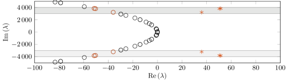
(a) Spectrum of first-order realization with selected interpolation points.

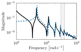
(b) Transfer functions.

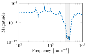
(c) Relative approximation error.

Figure 1: Approximation of a model in a specified frequency region $\Omega$. Only mirror images with respect to the imaginary axis of poles in the specified frequency region are considered leading to an accurate local approximation of the transfer function.

Reduced-order models computed with the structure-preserving framework presented in Section 2.1 approximate the full-order model well in the vicinity of chosen interpolation points. This observation can be used to compute reduced-order models, which approximate the original model in a specific frequency region only. Additionally, IRKA-like methods aim for interpolation at the mirror images of system poles with respect to the imaginary axis. Figure 1 illustrates the combination of these two ideas. The part of the spectrum of the model close to the imaginary axis is shown in Figure 1(a) and all eigenvalues $\lambda_{j}$ with $3000<\lvert\operatorname{Im}\left(\lambda_{j}\right)\rvert<4000$ are marked, which corresponds to the frequency region of interest $\Omega=[3000,4000]$ $\text{\,}\mathrm{rad}\text{\,}{\mathrm{s}}^{-1}$. The mirror images of these eigenvalues are considered as interpolation points in StrAIKA for the structure-preserving interpolation framework. The transfer function of the interpolating structured reduced-order model is shown in Figure 1(b) with the pointwise relative approximation error in Figure 1(c). It can be seen that the reduced-order model is an accurate approximation of the original system in the vicinity of the interpolation points $\sigma_{j}$. Choosing only interpolation points in the frequency region $\Omega$, which is important for the application of the reduced-order model, can therefore be a strategy to decrease the required size of the reduced-order model.

Note that there are no limitations for the choice of $\Omega$. For the global approach, it can be chosen to be the complete positive real axis $\mathbb{R}_{\geq 0}$ but in other applications, only subintervals might be of interest such that

$$\Omega=\bigcup\limits_{j=1}^{k}[\omega_{1,j},\omega_{2,j}],$$

where $\omega_{1,j},\omega_{2,j}\in\mathbb{R}_{\geq 0}$ and $\omega_{1,j}\leq\omega_{2,j}$. In 8 of Algorithm 3, the absolute value of the imaginary part of the eigenvalues is considered, which implies a certain symmetry in importance of positive and negative frequency regions; see also Figure 1(a). For certain applications, it may be advantageous to select eigenvalues using other criteria, for example, their distance to the imaginary axis.

In principle, the reduced-order model might grow too large if all interpolation points inside a defined region are considered. Especially in cases where the global dynamics are approximated, the order $r$ can grow fast and even approach $n$. For such cases, StrAIKA chooses eigenvalues up to a defined maximum $r_{\mathrm{max}}$ as locations for interpolation points. In this case, the $r_{\mathrm{max}}$ interpolation points, which will result in a suitably good approximation of the original model, have to be selected from all potential interpolation points. To this end, the dominance of all poles given by the eigenvalues in $\Omega$ is computed and, for the $r_{\mathrm{max}}$ most dominant poles, the interpolation points for the next iteration are set as their mirror images. The systems constructed in 8 of Algorithm 3 are in first-order unstructured form Eq. 3. For such systems, the dominance of a pole $\lambda_{j}$ with corresponding right and left eigenvectors $\boldsymbol{x}_{j}$ and $\boldsymbol{y}_{j}$ is defined as

$$d_{j}=\frac{\left\lVert\lambda_{j}(\boldsymbol{C}_{\mathbb{L}}\boldsymbol{y}_{j})(\boldsymbol{x}_{j}^{\mathsf{H}}\boldsymbol{B}_{\mathbb{L}})\right\rVert_{2}}{\lvert\operatorname{Re}\left(\lambda_{j}\right)\rvert};$$ (17)

where $\boldsymbol{C}_{\mathbb{L}}$ and $\boldsymbol{B}_{\mathbb{L}}$ are the output and input matrices constructed in 8 of Algorithm 3, respectively. A pole $\lambda_{j}$ is called dominant, if $d_{j}>d_{k}$ for all $j\neq k$; see [38].

To ensure a high approximation quality in the frequency range of interest $\Omega$, it is often beneficial to include also the first potential interpolation points located outside both ends of $\Omega$. While having only a small impact on the size of the reduced-order model, this can greatly increase the accuracy of the reduced-order model, especially, if the full-order model has poles near the boundaries of $\Omega$.

4 Numerical experiments

We now demonstrate the performance of StrAIKA in comparison with the established IRKA-like methods TF-IRKA and SPTF-IRKA. Where applicable, the classical IRKA is also included in the comparison. The numerical experiments have been performed on a laptop equipped with an AMD Ryzen™ 7 PRO 5850U and $12\text{\,}\mathrm{GB}$ RAM running on Linux Mint 21 as operating system. All algorithms have been implemented and run with MATLAB^® version 9.11.0.1837725 (R2021b Update 2). The results for IRKA have been computed with M-M.E.S.S. version 2.2 [43]. The source code, data and results of the numerical experiments are available at [8].

In all experiments, we use a maximum number of iterations: $n_{\mathrm{iter,max}}=50$ for StrAIKA and the outer iterations of SPTF-IRKA, and $n_{\mathrm{iter,max}}=100$ for TF-IRKA and the inner iterations of SPTF-IRKA. The algorithms terminate, if the relative difference between the interpolation points in two consecutive iterations falls under the threshold of $\epsilon=$1\text{$\cdot$}{10}^{-3}$$. To compare the accuracy of the methods, we plot the pointwise relative approximation errors, given by

$$\operatorname{relerr}(\omega):=\frac{\lVert\boldsymbol{H}(\mathfrak{i}\omega)-{\hstretch{2.5}{\hat{\hstretch{.4}{\boldsymbol{H}\mkern 4.0mu}}}\mkern-4.0mu}{}(\mathfrak{i}\omega)\|_{2}}{\lVert\boldsymbol{H}(\mathfrak{i}\omega)\rVert_{2}}$$

in specified frequency intervals of interest $\omega\in[\omega_{\min},\omega_{\max}]$. We also we approximate the local, relative errors in $\Omega$ under the $\mathcal{L}_{\infty}$-norm via

$$\operatorname{relerr}_{\mathcal{L}_{\infty},\Omega}=\frac{\max\limits_{\omega\in\Omega}\lVert\boldsymbol{H}(\mathfrak{i}\omega)-{\hstretch{2.5}{\hat{\hstretch{.4}{\boldsymbol{H}\mkern 4.0mu}}}\mkern-4.0mu}{}(\mathfrak{i}\omega)\lVert_{2}}{\max\limits_{\omega\in\Omega}\lVert\boldsymbol{H}(\mathfrak{i}\omega)\lVert_{2}}\approx\frac{\lVert\boldsymbol{H}-{\hstretch{2.5}{\hat{\hstretch{.4}{\boldsymbol{H}\mkern 4.0mu}}}\mkern-4.0mu}{}\rVert_{\mathcal{L}_{\infty},\Omega}}{\lVert\boldsymbol{H}\rVert_{\mathcal{L}_{\infty},\Omega}},$$

using equidistant discretizations of $\Omega$.

4.1 Unstructured first-order system example

In the first example, we consider a system modeling the structural response of the Russian Service Module of the International Space Station (ISS) [30]. The system is modeled using first-order differential equations Eq. 3 and has $n=270$ states, $m=3$ inputs and $p=3$ outputs. The transfer function is given by

$$\boldsymbol{H}(s)=\boldsymbol{C}\left(s\boldsymbol{E}-\boldsymbol{A}\right)^{-1}\boldsymbol{B}.$$

The model is evaluated for frequencies in the range $\Omega=\left[$1\text{$\cdot$}{10}^{-2}$,$1\text{$\cdot$}{10}^{3}$\right]$ $\text{\,}\mathrm{rad}\text{\,}{\mathrm{s}}^{-1}$. Because of the first-order structure of the full-order model, IRKA can be applied in this case. Additionally, TF-IRKA, SPTF-IRKA and StrAIKA are employed to compute real-valued reduced-order models of size $r=20$ each. Sigma plots of the transfer functions and relative approximation errors for all models are given in Figure 2. Table 1 summarizes the performance of the algorithms.

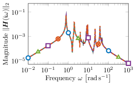
(a) Transfer functions.

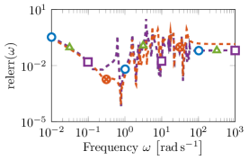
(b) Relative errors.

Figure 2: First-order system example: All applied methods provide a similar approximation behavior since no special structure needs to be preserved in the example. Insignificant differences are revealed by the pointwise relative errors.

Table 1: First-order system example: Comparisons of the relative, local $\mathcal{L}_{\infty}$-errors, the required number of iterations $n_{\mathrm{iter}}$, the number of solutions of full-order $n$ linear system $n_{\mathrm{ls}}$ and the computation time $t_{\mathrm{c}}$.

Algorithm	$\operatorname{relerr}_{\mathcal{L}_{\infty},\Omega}$	$n$iter	$n$ls	$t$c$\left[$\mathrm{s}$\right]$
StrAIKA	$0.036\,692\,542\,730\,048\,1$	$21$	$222$	$1.917\,002$
TF-IRKA	$0.036\,692\,542\,528\,399\,7$	$10$	$200$	$0.181\,644$
SPTF-IRKA	$0.036\,692\,542\,516\,082\,4$	$12$	$132$	$0.265\,119$
IRKA	$0.042\,171\,936\,459\,93$	$13$	$130$	$0.169\,957$

All employed methods succeed in computing surrogates, which approximate the original system up to the same degree of accuracy. Only IRKA obtains a different local optimum than the other methods, which yields an insignificantly larger relative approximation error; cf. Table 1. This meets expectations, as the first-order structure of the original system can be represented well by the realization TF-IRKA yields. TF-IRKA converges after only ten iterations, while the other methods require more. IRKA performs the fewest decompositions of the full-order matrices and has the shortest runtime; however, the significance of the runtime is limited for this small example. StrAIKA requires the most iterations and therefore the most matrix decompositions. The runtime is longer than for the other methods. This is a result of the additional sampling step performed in each iteration of StrAIKA, which has a measurable influence on the runtime, as $n$ is relatively small in comparison to $r$ in this example.

4.2 Time-delayed heated rod

Here, we consider a model of a heated rod with distributed control and homogeneous Dirichlet boundary conditions, which is cooled by delayed feedback. This system has also been analyzed in [15]. A discretization of the underlying partial differential equation leads to the transfer function

$$\boldsymbol{H}(s)=\boldsymbol{C}\left(s\boldsymbol{E}-\boldsymbol{A}_{0}-\operatorname{e}^{-\tau s}\boldsymbol{A}_{\mathrm{d}}\right)^{-1}\boldsymbol{B},$$

with $n=1\,000\,000$ states, $m=5$ inputs and $p=4$ outputs. The time delay is $\tau=1$ in this example. The input matrix $\boldsymbol{B}$ has a block structure such that the rod is heated uniformly at different sections by the inputs. The outputs are the average temperatures on these sections. For this example, the frequency range $\Omega=\left[$1\text{$\cdot$}{10}^{-4}$,$1\text{$\cdot$}{10}^{4}$\right]$ $\text{\,}\mathrm{rad}\text{\,}{\mathrm{s}}^{-1}$ is considered. For the experiments, we fix the reduced order to $r=10$ and compute reduced-order models with StrAIKA, TF-IRKA and SPTF-IRKA. The system cannot be transformed into an equivalent system with first-order structure, therefore IRKA cannot be applied in this case. The initial interpolation points are distributed linearly equidistant in $\mathfrak{i}\left[$1\text{$\cdot$}{10}^{-4}$,$1\text{$\cdot$}{10}^{2}$\right]$. Figure 3 plots the maximum singular values of the transfer functions and the error systems. Further results are given in Table 2.

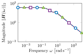
(a) Transfer functions.

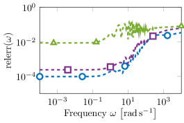
(b) Relative errors.

Figure 3: Time-delay system example: The unstructured approximation computed by TF-IRKA is around two orders of magnitude less accurate than the structure-preserving reduced-order models computed by StrAIKA and SPTF-IRKA for smaller to medium frequencies. Overall StrAIKA provides the most accurate approximation.

Table 2: Time-delay system example: Comparisons of the relative, local $\mathcal{L}_{\infty}$-errors, the required number of iterations $n_{\mathrm{iter}}$, the number of solutions of full-order $n$ linear system $n_{\mathrm{ls}}$ and the computation time $t_{\mathrm{c}}$.

Algorithm	$\operatorname{relerr}_{\mathcal{L}_{\infty},\Omega}$	$n$iter	$n$ls	$t$c$\left[$\mathrm{s}$\right]$
StrAIKA	$0.000\,101\,105\,936\,687\,689$	$37$	$190$	$247.101\,835$
TF-IRKA	$0.020\,574\,550\,747\,899$	$73$	$730$	$367.244\,314$
SPTF-IRKA	$0.000\,238\,103\,757\,728\,217$	$3$	$29$	$37.562\,543$

In this example, StrAIKA and SPTF-IRKA compute reduced-order models with comparable accuracy. However, StrAIKA provides the smallest worst case error by around a factor of two as shown in Table 2. As expected, the first-order realization computed by TF-IRKA cannot capture the dynamics of the delay system well and, therefore, provides an approximation that is around two orders of magnitude less accurate than the models computed by StrAIKA and SPTF-IRKA. Because of its rapid convergence, the runtime of SPTF-IRKA is considerably lower than for the other two algorithms. But also the runtime of StrAIKA is significantly smaller than for TF-IRKA. Note, that most of the system dynamics happen in the considered frequency range. Therefore, StrAIKA quickly reaches the maximum reduced order and has to choose the $10$ most dominant poles out of approximately $150$ eigenvalues of the Loewner realization in each iteration. This additional effort directly affects the runtime of StrAIKA. Additionally, the convergence is slow compared to SPTF-IRKA.

4.3 Viscoelastic beam

This example models a flexible beam with viscoelastic core. The beam of length $l=$0.21\text{\,}\mathrm{m}$$ has a symmetric sandwich structure consisting of two layers of cold rolled steel surrounding a viscoelastic ethylene-propylene-diene core [47]; the beam is clamped at one side. After discretization, the transfer function of the system is given by

$$\boldsymbol{H}(s)=\boldsymbol{C}\left(s^{2}\boldsymbol{M}+\boldsymbol{K}+\frac{G_{0}+G_{\infty}\left(s\tau\right)^{\alpha}}{1+\left(s\tau\right)^{\alpha}}\boldsymbol{G}\right)^{-1}\boldsymbol{B}.$$

The model has $n=3\,360$ states, $m=1$ input and $p=1$ output. The beam is excited by a single load at its free end and the displacement is measured at the same location, resulting in output and input mappings $\boldsymbol{C}=100\cdot\boldsymbol{B}^{\mkern-1.5mu\mathsf{T}}=\begin{bmatrix}0&\cdots&0&1\end{bmatrix}$. The matrices $\boldsymbol{M}$, $\boldsymbol{K}$, $\boldsymbol{G}$ are available from [35]. In this example, we limit the frequency range of interest to $\Omega=\left[$10$,$1\text{$\cdot$}{10}^{4}$\right]$ $\text{\,}\mathrm{rad}\text{\,}{\mathrm{s}}^{-1}$. Note, that the system has poles, which lie outside of this range. No maximum reduced order $r$ is set in this case, so StrAIKA determines it in an adaptive way. The initial interpolation points are a single complex conjugate pair, where the absolute value of its imaginary part is located in the middle of $\Omega$. The automatically determined order is used for the experiments with TF-IRKA and SPTF-IRKA, where the $\lceil r/2\rceil$ initial expansion points and their complex conjugates are distributed logarithmically equidistant in $\Omega$. The sigma plots for the frequency responses of the reference and the reduced-order models as well as the corresponding errors are given in Figure 4. The performance of the methods is shown in Table 3.

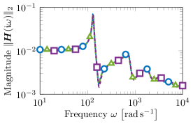
(a) Transfer functions.

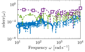
(b) Relative errors.

Figure 4: Viscoelastic beam example: All methods succeed in computing reasonably accurate reduced-order models. The relative approximation error of the reduced-order model obtained by StrAIKA is around three orders of magnitude smaller compared to the other methods.

Table 3: Viscoelastic beam example: Comparisons of the relative, local $\mathcal{L}_{\infty}$-errors, the required number of iterations $n_{\mathrm{iter}}$, the number of solutions of full-order $n$ linear system $n_{\mathrm{ls}}$ and the computation time $t_{\mathrm{c}}$. The $\ast$ marks experiments, where the maximum number of iterations has been reached without convergence.

Algorithm	$\operatorname{relerr}_{\mathcal{L}_{\infty},\Omega}$	$n$iter	$n$ls	$t$c$\left[$\mathrm{s}$\right]$
StrAIKA	$0.000\,913\,874\,693\,057\,171$	$10$	$74$	$0.709\,724$
TF-IRKA	$0.001\,036\,721\,284\,719\,25$	$18$	$288$	$0.970\,171$
SPTF-IRKA	$0.009\,596\,887\,571\,169\,32$	$50$	$457$	$8.276\,918$	$\ast$

StrAIKA converges after ten iterations to a model of size $r=15$, i.e., the reduced-order models computed by TF-IRKA and SPTF-IRKA have order $r=16$. All three algorithms produce reasonably accurate models regarding the reference, while the model computed by StrAIKA is around three orders of magnitude more accurate for most frequencies; cf. Figure 4(b). Also the worst case approximation error of StrAIKA is around one order of magnitude better than SPTF-IRKA; see Table 3. This can be explained by the fact that StrAIKA places all interpolation points in $\Omega$, while some of the interpolation points obtained by the other two algorithms are located in the frequency region above $1\text{$\cdot$}{10}^{4}\text{\,}\mathrm{rad}\text{\,}{\mathrm{s}}^{-1}$, leading to a higher error in $\Omega$. SPTF-IRKA did not converge after $50$ iterations, resulting in a high computation time. In terms of computational effort, StrAIKA is clearly advantageous in this example.

4.4 Radio frequency gun

As the last example, we consider a radio frequency gun as described in [37]. Discretizing the system leads to a transfer function

$$\boldsymbol{H}(s)=\boldsymbol{C}\left(s^{2}\boldsymbol{M}+\mathfrak{i}\left(s^{2}-\sigma_{1}^{2}\right)^{\frac{1}{2}}\boldsymbol{W}_{1}+\mathfrak{i}\left(s^{2}-\sigma_{2}^{2}\right)^{\frac{1}{2}}\boldsymbol{W}_{2}+\boldsymbol{K}\right)^{-1}\boldsymbol{B},$$

where $\sigma_{1}=0.0$ and $\sigma_{2}=108.8774$. The full-order model has $n=9\,956$ states and the matrices $\boldsymbol{M},\boldsymbol{W}_{1},\boldsymbol{W}_{2},\boldsymbol{K}$ are taken from [35]. We consider $m=1$ input and $p=1$ output. The input vector is populated with values drawn from the standard normal distribution and the system output is measured at the first degree of freedom, corresponding to $\boldsymbol{C}=\begin{bmatrix}1&0&\ldots&0\end{bmatrix}$. These vectors are also part of the code package supplementing this article [8]. The reduced-order models are computed to approximate the original system in $\Omega=\left[1,160\right]$ $\text{\,}\mathrm{rad}\text{\,}{\mathrm{s}}^{-1}$ and the necessary order $r$ for the surrogate is automatically determined by StrAIKA. One initial complex conjugate pair of interpolation points is placed in the middle of $\Omega$. The initial $\lceil r/2\rceil$ pairs of interpolation points for TF-IRKA and SPTF-IRKA are distributed linearly equidistant in $\Omega$. The sigma plots for the frequency responses of the reference and the reduced-order models as well as the corresponding relative approximation errors are shown in Figure 5. The local, relative $\mathcal{L}_{\infty}$-errors and computational costs are presented in Table 4.

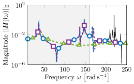
(a) Transfer functions.

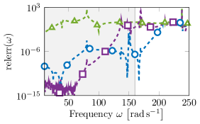
(b) Relative errors.

Figure 5: Radio frequency gun example: The reduced-order model computed by StrAIKA shows a relatively uniform accuracy in $\Omega$, while the surrogate obtained form SPTF-IRKA is only accurate for less than $60\text{\,}\mathrm{rad}\text{\,}{\mathrm{s}}^{-1}$. The first-order system computed by TF-IRKA is not able to approximate the dynamics of the original system at all.

Table 4: Radio frequency gun example: Comparisons of the relative, local $\mathcal{L}_{\infty}$-errors, the required number of iterations $n_{\mathrm{iter}}$, the number of solutions of full-order $n$ linear system $n_{\mathrm{ls}}$ and the computation time $t_{\mathrm{c}}$. The $\ast$ marks experiments, where the maximum number of iterations has been reached without convergence.

Algorithm	$\operatorname{relerr}_{\mathcal{L}_{\infty},\Omega}$	$n$iter	$n$ls	$t$c$\left[$\mathrm{s}$\right]$
StrAIKA	$0.000\,173\,015\,039\,226\,412$	$50$	$416$	$123.327\,627$	$\ast$
TF-IRKA	$0.999\,844\,667\,946\,225$	$100$	$3000$	$2909.537\,882$	$\ast$
SPTF-IRKA	$0.999\,775\,790\,485\,055$	$50$	$1316$	$392.115\,224$	$\ast$

StrAIKA automatically determines a reduced order of $r=30$ and computes a reduced-order model, which is more accurate in the frequency range of interest than the reduced-order models computed by the other two algorithms. Placing the interpolation points only inside $\Omega$ leads to a higher accuracy in this region, while the approximation deteriorates for higher frequencies. Although StrAIKA does not converge after 50 iterations, the reduced-order model is more than reasonably accurate, with its worst case approximation error being four orders of magnitude smaller than for the other methods; see Table 4. The other two methods also do not converge in the allowed number of iterations. This example clearly shows the increased computational effort required for TF-IRKA as well as SPTF-IRKA. In particular, SPTF-IRKA takes more than three times longer than StrAIKA for the same number of iterations. This is a result of the large number of iterations required for the inner TF-IRKA inside of SPTF-IRKA leading to a large number of linear solves to be performed. The unstructured TF-IRKA fails in computing a surrogate that approximates the transfer function of the full-order model. The reduced-order model computed by SPTF-IRKA approximates the full-order model well in the lower frequency region, but the overall accuracy in $\Omega$ is lower than observed for the model computed by StrAIKA. The comparison to TF-IRKA again shows the importance of structure-preserving model order reduction strategies.

5 Conclusions

In this paper, we proposed StrAIKA, a new algorithm that computes structure-preserving reduced-order models of systems with arbitrary transfer function structure in an iterative way. Similar to IRKA-like methods, StrAIKA uses mirror images of intermediate reduced-order models as interpolation points for the next iteration. In each iteration, the Loewner framework is used to compute first-order realizations of transfer function data collected from the current reduced-order model, whose eigenvalues are the basis for the interpolation points in the next iteration. StrAIKA automatically determines a size for the reduced-order model by considering the eigenvalues located in a given frequency range of interest. This ensures a reasonable approximation of the system dynamics at least in these regions. StrAIKA is completely agnostic to the actual transfer function structure of the original model and does not require any transfer function derivatives.

We demonstrated the versatility and effectiveness of StrAIKA in four numerical examples with different internal structures. The benchmark systems model structural vibration, heat transfer with internal delay, viscoelasticity, and radio wave propagation. StrAIKA showed comparable or even significantly better accuracy with respect to established IRKA-like methods. Especially, if only a limited frequency range is of interest for the application, StrAIKA easily outperforms methods that optimize the approximation error under the $\mathcal{H}_{2}$-norm both in terms of accuracy and required computational effort.

An open question that has not been covered in this paper is the preservation of additional system properties like stability. However, the preservation of such system properties has only been solved for particular system structures such as first-order systems or second-order systems with mechanical matrix structure. For the case of generally structured systems as considered in this paper, no solution to this problem for projection-based model reduction is known yet. Another idea for future investigations is the reduction of the computational costs of StrAIKA by considering an additional layer of approximation as it has been done for IRKA-like methods in [6, 18].

References

- [1] R. Abraham and J. E. Marsden. Foundations of Mechanics. Addison-Wesley Publishing Company, Inc., Redwood City, second edition, 1987. URL: https://resolver.caltech.edu/CaltechBOOK:1987.001.
- [2] N. Aliyev, P. Benner, E. Mengi, and M. Voigt. A subspace framework for -norm minimization. SIAM J. Matrix Anal. Appl., 41(2):928–956, 2020. doi:10.1137/19M125892X.
- [3] A. C. Antoulas. Approximation of Large-Scale Dynamical Systems, volume 6 of Adv. Des. Control. SIAM, Philadelphia, PA, 2005. doi:10.1137/1.9780898718713.
- [4] A. C. Antoulas, S. Lefteriu, and A. C. Ionita. A tutorial introduction to the Loewner framework for model reduction. In P. Benner, M. Ohlberger, A. Cohen, and K. Willcox, editors, Model Reduction and Approximation: Theory and Algorithms, Computational Science & Engineering, pages 335–376. SIAM, Philadelphia, PA, 2017. doi:10.1137/1.9781611974829.ch8.
- [5] Q. Aumann, E. Deckers, S. Jonckheere, W. Desmet, and G. Müller. Automatic model order reduction for systems with frequency-dependent material properties. Comput. Methods Appl. Mech. Eng., 397:115076, 2022. doi:10.1016/j.cma.2022.115076.
- [6] Q. Aumann and G. Müller. An adaptive method for reducing second-order dynamical systems. IFAC-Pap., 55(20):337–342, 2022. 10th Vienna International Conference on Mathematical Modelling MATHMOD 2022. doi:10.1016/j.ifacol.2022.09.118.
- [7] Q. Aumann and G. Müller. Robust error assessment for reduced order vibro-acoustic problems. J. Sound Vib., 545:117427, 2023. doi:10.1016/j.jsv.2022.117427.
- [8] Q. Aumann and S. W. R. Werner. Code, data and results for the numerical experiments in “Adaptive choice of near-optimal expansion points for interpolation-based structure-preserving model reduction” (version 1.0), April 2023. doi:10.5281/zenodo.7845175.
- [9] Q. Aumann and S. W. R. Werner. Structured model order reduction for vibro-acoustic problems using interpolation and balancing methods. J. Sound Vib., 543:117363, 2023. doi:10.1016/j.jsv.2022.117363.
- [10] C. A. Beattie and S. Gugercin. Interpolatory projection methods for structure-preserving model reduction. Syst. Control Lett., 58(3):225–232, 2009. doi:10.1016/j.sysconle.2008.10.016.
- [11] C. A. Beattie and S. Gugercin. Realization-independent -approximation. In 51st IEEE Conference on Decision and Control (CDC), pages 4953–4958, 2012. doi:10.1109/CDC.2012.6426344.
- [12] R. S. Beddig, P. Benner, I. Dorschky, T. Reis, P. Schwerdtner, M. Voigt, and S. W. R. Werner. Structure-preserving model reduction for dissipative mechanical systems. e-print 2010.06331, arXiv, 2020. Optimization and Control (math.OC). doi:10.48550/arXiv.2010.06331.
- [13] T. Bendokat and R. Zimmermann. Geometric optimization for structure-preserving model reduction of Hamiltonian systems. IFAC-Pap., 55(20):457–462, 2022. 10th Vienna International Conference on Mathematical Modelling MATHMOD 2022. doi:10.1016/j.ifacol.2022.09.137.
- [14] P. Benner, S. Grundel, and N. Hornung. Parametric model order reduction with a small -error using radial basis functions. Adv. Comput. Math., 41(5):1231–1253, 2015. doi:10.1007/s10444-015-9410-7.
- [15] P. Benner, S. Gugercin, and S. W .R. Werner. A unifying framework for tangential interpolation of structured bilinear control systems. e-print 2206.01657, arXiv, 2022. Numerical Analysis (math.NA). doi:10.48550/arXiv.2206.01657.
- [16] M. Berljafa and S. Güttel. The RKFIT algorithm for nonlinear rational approximation. SIAM J. Sci. Comput., 39(5):A2049–A2071, 2017. doi:10.1137/15M1025426.
- [17] T. Bonin, H. Faßbender, A. Soppa, and M. Zaeh. A fully adaptive rational global Arnoldi method for the model-order reduction of second-order MIMO systems with proportional damping. Math. Comput. Simul., 122:1–19, 2016. doi:10.1016/j.matcom.2015.08.017.
- [18] A. Castagnotto and B. Lohmann. A new framework for -optimal model reduction. Math. Comput. Model. Dyn. Syst., 24(3):236–257, 2018. doi:10.1080/13873954.2018.1464030.
- [19] S. Chellappa, L. Feng, and P. Benner. An adaptive sampling approach for the reduced basis method. In C. Beattie, P. Benner, M. Embree, S. Gugercin, and S. Lefteriu, editors, Realization and Model Reduction of Dynamical Systems, pages 137–155. Springer, Cham, 2022. doi:10.1007/978-3-030-95157-3_8.
- [20] X. Cheng, Y. Kawano, and J. M. A. Scherpen. Reduction of second-order network systems with structure preservation. IEEE Trans. Autom. Control, 62(10):5026–5038, 2017. doi:10.1109/TAC.2017.2679479.
- [21] G. Cohen, A. Hauck, M. Kaltenbacher, and T. Otsuru. Different types of finite elements. In S. Marburg and B. Nolte, editors, Computational Acoustics of Noise Propagation in Fluids – Finite and Boundary Element Methods, pages 57–88. Springer, Berlin, Heidelberg, 2008. doi:10.1007/978-3-540-77448-8_3.
- [22] E. Deckers, W. Desmet, K. Meerbergen, and F. Naets. Case studies of model order reduction for acoustics and vibrations. In P. Benner, W. Schilders, S. Grivet-Talocia, A. Quarteroni, G. Rozza, and L. M. Silveira, editors, Model Order Reduction. Volume 3: Applications, pages 76–110. De Gruyter, Berlin, Boston, 2021. doi:10.1515/9783110499001-003.
- [23] Z. Drmač, S. Gugercin, and C. Beattie. Quadrature-based vector fitting for discretized approximation. SIAM J. Sci. Comput., 37(2):A625–A652, 2015. doi:10.1137/140961511.
- [24] H. Egger, T. Kugler, B. Liljegren-Sailer, M. Marheineke, and V. Mehrmann. On structure-preserving model reduction for damped wave propagation in transport networks. SIAM J. Sci. Comput., 40(1):A331–A365, 2018. doi:10.1137/17M1125303.
- [25] L. Feng, J. G. Korvink, and P. Benner. A fully adaptive scheme for model order reduction based on moment matching. IEEE Trans. Compon. Packag. Manuf. Technol., 5(12):1872–1884, 2015. doi:10.1109/TCPMT.2015.2491341.
- [26] L. Feng, L. Lombardi, P. Benner, D. Romano, and G. Antonini. Model order reduction for delayed PEEC models with guaranteed accuracy and observed stability. IEEE Trans. Circuits Syst. I: Regul. Pap., 69(10):4177–4190, 2022. doi:10.1109/TCSI.2022.3189389.
- [27] Q. Gao and H. R. Karimi. Stability, Control and Application of Time-delay Systems. Butterworth-Heinemann, Oxford, 2019. doi:10.1016/C2017-0-02175-4.
- [28] I. V. Gosea, S. Gugercin, and S. W. R. Werner. Structured barycentric forms for interpolation-based data-driven reduced modeling of second-order systems. e-print 2303.12576, arXiv, 2023. Numerical Analysis (math.NA). doi:10.48550/arXiv.2303.12576.
- [29] S. Gugercin, A. C. Antoulas, and C. Beattie. model reduction for large-scale linear dynamical systems. SIAM J. Matrix Anal. Appl., 30(2):609–638, 2008. doi:10.1137/060666123.
- [30] S. Gugercin, A. C. Antoulas, and M. Bedrossian. Approximation of the international space station 1R and 12A models. In Proceedings of the 40th IEEE Conference on Decision and Control, pages 1515–1516, 2001. doi:10.1109/CDC.2001.981109.
- [31] S. Gugercin, R. V. Polyuga, C. Beattie, and A. Van der Schaft. Structure-preserving tangential interpolation for model reduction of port-Hamiltonian systems. Automatica J. IFAC, 48(9):1963–1974, 2012. doi:10.1016/j.automatica.2012.05.052.
- [32] B. Gustavsen and A. Semlyen. Rational approximation of frequency domain responses by vector fitting. IEEE Trans. Power Del., 14(3):1052–1061, 1999. doi:10.1109/61.772353.
- [33] J. S. Hesthaven, C. Pagliantini, and N. Ripamonti. Rank-adaptive structure-preserving model order reduction of Hamiltonian systems. ESAIM: Math. Model. Numer. Anal., 56(2):617–650, 2022. doi:10.1051/m2an/2022013.
- [34] U. Hetmaniuk, R. Tezaur, and C. Farhat. Review and assessment of interpolatory model order reduction methods for frequency response structural dynamics and acoustics problems. Int. J. Numer. Methods Eng., 90(13):1636–1662, 2012. doi:10.1002/nme.4271.
- [35] N. J. Higham, G. M. Negri Porzio, and F. Tisseur. An updated set of nonlinear eigenvalue problems. e-print 2019.5, MIMS, 2019. My Class (my.class). URL: http://eprints.maths.manchester.ac.uk/id/eprint/2699.
- [36] D. S. Karachalios, I. V. Gosea, and A. C. Antoulas. The Loewner framework for system identification and reduction. In P. Benner, W. Schilders, S. Grivet-Talocia, A. Quarteroni, G. Rozza, and L. M. Silveira, editors, Model Order Reduction. Volume 1: System- and Data-Driven Methods and Algorithms, pages 181–228. De Gruyter, Berlin, Boston, 2021. doi:10.1515/9783110498967-006.
- [37] B.-S. Liao. Subspace Projection Methods for Model Order Reduction and Nonlinear Eigenvalue Computation. Dissertation, University of California, Davis, California, USA, 2007.
- [38] N. Martins, L. T. G. Lima, and H. J. C. P. Pinto. Computing dominant poles of power system transfer functions. IEEE Trans. Power Syst., 11(1):162–170, 1996. doi:10.1109/59.486093.
- [39] A. J. Mayo and A. C. Antoulas. A framework for the solution of the generalized realization problem. Linear Algebra Appl., 425(2–3):634–662, 2007. Special issue in honor of P. A. Fuhrmann, Edited by A. C. Antoulas, U. Helmke, J. Rosenthal, V. Vinnikov, and E. Zerz. doi:10.1016/j.laa.2007.03.008.
- [40] Y. Nakatsukasa, O. Sète, and L. N. Trefethen. The AAA algorithm for rational approximation. SIAM J. Sci. Comput., 40(3):A1494–A1522, 2018. doi:10.1137/16M1106122.
- [41] H. K. F. Panzer, T. Wolf, and B. Lohmann. and error bounds for model order reduction of second order systems by Krylov subspace methods. In 2013 European Control Conference (ECC), pages 4484–4489, 2013. doi:10.23919/ECC.2013.6669657.
- [42] R. Rumpler, P. Göransson, and J.-F. Deü. A finite element approach combining a reduced‐order system, Padé approximants, and an adaptive frequency windowing for fast multi‐frequency solution of poro‐acoustic problems. Int. J. Numer. Methods Eng., 97(10):759–784, 2014. doi:10.1002/nme.4609.
- [43] J. Saak, M. Köhler, and P. Benner. M-M.E.S.S. – The Matrix Equations Sparse Solvers library (version 2.2), February 2022. see also: https://www.mpi-magdeburg.mpg.de/projects/mess. doi:10.5281/zenodo.5938237.
- [44] P. Schulze, B. Unger, C. Beattie, and S. Gugercin. Data-driven structured realization. Linear Algebra Appl., 537:250–286, 2018. doi:10.1016/j.laa.2017.09.030.
- [45] P. Schwerdtner and M. Voigt. Adaptive sampling for structure-preserving model order reduction of port-Hamiltonian systems. IFAC-Pap., 54(19):143–148, 2021. 7th IFAC Workshop on Lagrangian and Hamiltonian Methods for Nonlinear Control LHMNC 2021. doi:10.1016/j.ifacol.2021.11.069.
- [46] K. Sinani, S. Gugercin, and C. Beattie. A structure-preserving model reduction algorithm for dynamical systems with nonlinear frequency dependence. IFAC-Pap., 49(9):56–61, 2016. 6th IFAC Symposium on System Structure and Control SSSC 2016. doi:10.1016/j.ifacol.2016.07.492.
- [47] R. Van Beeumen, K. Meerbergen, and W. Michiels. A rational Krylov method based on Hermite interpolation for nonlinear eigenvalue problems. SIAM J. Sci. Comput., 35(1):A327–A350, 2013. doi:10.1137/120877556.
- [48] P. Vuillemin, C. Poussot-Vassal, and D. Alazard. optimal and frequency limited approximation methods for large-scale LTI dynamical systems. IFAC Proceedings Volumes, 46(2):719–724, 2013. 5th IFAC Symposium on System Structure and Control. doi:10.3182/20130204-3-FR-2033.00061.
- [49] S. W. R. Werner. Structure-Preserving Model Reduction for Mechanical Systems. Dissertation, Otto-von-Guericke-Universität, Magdeburg, Germany, 2021. doi:10.25673/38617.
- [50] S. W. R. Werner, I. V. Gosea, and S. Gugercin. Structured vector fitting framework for mechanical systems. IFAC-Pap., 55(20):163–168, 2022. 10th Vienna International Conference on Mathematical Modelling MATHMOD 2022. doi:10.1016/j.ifacol.2022.09.089.
- [51] K. Wu. Power Converters with Digital Filter Feedback Control. Academic Press, London, 2016. doi:10.1016/C2015-0-01103-0.
- [52] S. Wyatt. Issues in Interpolatory Model Reduction: Inexact Solves, Second-order Systems and DAEs. PhD thesis, Virginia Polytechnic Institute and State University, Blacksburg, Virginia, USA, 2012. URL: http://hdl.handle.net/10919/27668.