Supercloseness of the LDG method for a two-dimensional singularly perturbed convection-diffusion problem on Bakhvalov-type mesh

Abstract

In this paper, we focus on analyzing the supercloseness property of a two-dimensional singularly perturbed convection-diffusion problem with exponential boundary layers. The local discontinuous Galerkin (LDG) method with piecewise tensor-product polynomials of degree $k$ is applied to Bakhvalov-type mesh. By developing special two-dimensional local Gauss-Radau projections and establishing a novel interpolation, supercloseness of an optimal order $k+1$ can be achieved on Bakhvalov-type mesh. It is crucial to highlight that this supercloseness result is independent of the singular perturbation parameter $\varepsilon$.

1 Introduction

Take the following two-dimensional singularly perturbed problem into consideration:

$$-\varepsilon\Delta u+\boldsymbol{\alpha}\cdot\nabla u+bu= f\quad \text{in $\Omega=(0,1)^{2}$},$$ (1)

$$u= 0\quad \text{on $\partial\Omega$},$$

where the coefficient $\varepsilon$ is a positive parameter, $\boldsymbol{\alpha}=\boldsymbol{\alpha}(x,y)$, $b=b(x,y)$ and $f=f(x,y)$ are sufficiently smooth and satisfy for $\forall(x,y)\in\bar{\Omega}$, $\boldsymbol{\alpha}(x,y)=(a_{1}(x,y),a_{2}(x,y))>(0,0),\quad b(x,y)-\frac{1}{2}\nabla\cdot\boldsymbol{\alpha}(x,y)>0$. Under these assumptions, utilizing the Lax-Milgram lemma allows for a demonstration of the existence of a unique weak solution in $H_{0}^{1}(\Omega)\cap H_{2}(\Omega)$ for equation (1). This solution typically includes two exponential layers of width $\mathcal{O}(\varepsilon\ln(1/\varepsilon))$ at $x=1$ and $y=1$.

Problem (1) can be viewed as a model for solving practical applications like the linearised Navier-Stokes equations at high Reynolds number [10]. It is widely known that the solution often exhibits a boundary layer, which is characterized by the fact that, although $u$ remains bounded, its derivatives might be significantly large within narrow regions adjacent to the boundary $\partial\Omega$. This situation undermines the stability and the efficiency of traditional numerical methods. Even on adequately refined, layer-adapted meshes, oscillations may persist. Therefore, numerous stabilized and efficient numerical methods have been put forth in order to obtain accurate results (see [10, 6, 8]).

In this manuscript, we employ the local discontinuous Galerkin (LDG) method [5], a type of finite element method known for its excellent stability and high order accuracy [13]. Owing to these characteristics, the LDG method is particularly suited for addressing singularly perturbed problems like (1). In recent years, there has been a surge of literature related to the application of the LDG method, as exemplified by [12, 15, 3, 2] and their respective references.

Supercloseness is a crucial convergence property for the LDG method, which denotes the difference between the LDG solution and a specific interpolation of the exact solution under certain norms. Investigations into supercloseness of the LDG method for singularly perturbed convection-diffusion problems have been conducted in [12, 11, 14, 4]. Building upon these studies, researchers have derived optimal supercloseness results on a series of layer-adapted meshes, including Shishkin-type and Bakhvalov-type meshes. When considering the two-dimensional case, however, few results have been established [18, 4], especially on Bakhvalov-type mesh. Difficulties arise from the construction of two-dimensional interpolation and the special width of the layer of Bakhvalov-type mesh.

For equation (1), Cheng et al. [4] applied the LDG method to systematically analyze supercloseness under an energy norm on various types of meshes. They demonstrated an optimal order of $k+1$ on Shishkin-type mesh and Bakhvalov-Shishkin-type mesh. However, on Bakhvalov-type mesh, their supercloseness result was $\mathcal{O}(N^{-(k+1)}\ln(1/\varepsilon)^{1/2})$, affected by the factor $(\ln(1/\varepsilon))^{1/2}$. This influence is caused by the special layer width $\mathcal{O}(\varepsilon\ln(1/\varepsilon))$ of Bakhvalov-type mesh. From a numerical analysis perspective, removing the factor $(\ln(1/\varepsilon))^{1/2}$ and obtaining the optimal convergence results that are independent of $\varepsilon$ on Bakhvalov-type mesh are very interesting and challenging. In the field of the standard finite element method, Roos [19, 21] and Zhang [20, 22] have successively accomplished uniform convergence and supercloseness, unaffected by $\varepsilon$, on Bakhvalov-type mesh by employing diverse techniques. Correspondingly, in the field of the LDG method, it is necessary to prove supercloseness unaffected by $\varepsilon$ on Bakhvalov-type mesh, that is, eliminate the factor $(\ln(1/\varepsilon))^{1/2}$ in the supercloseness result. However, existing interpolation methods or analytical techniques have not been able to effectively tackle this challenge.

To address this research gap, we first design special two-dimensional local Gauss-Radau projections. Subsequently, we construct a novel interpolation to eliminate the intractable element errors. This new interpolation utilizes the characteristics of the special projections and the structure of Bakhvalov-type mesh. Further contributing to the realization of the optimal supercloseness result is the implementation of some improved analytical techniques. In conclusion, supercloseness of an optimal order $k+1$ under the energy norm can be achieved on Bakhvalov-type mesh, independent of the singular perturbation parameter $\varepsilon$. Our article successfully removes the factor $(\ln(1/\varepsilon))^{1/2}$ and proves a parameter-uniform supercloseness result on Bakhvalov-type mesh, indicating an effective analysis to tackle the issues associated with singularly perturbed convection-diffusion problems of the LDG method in 2D.

This paper is organized as follows: In Section 2, we present some regularity results of the solution to problem (1), describe Bakhvalov-type mesh, and introduce the LDG method. In Section 3, special two-dimensional local Gauss-Radau projections are defined, and a novel interpolation is established. Besides, some preliminary results are also presented in this section. Finally, the supercloseness property under the energy norm is thoroughly demonstrated in Section 4.

General constant $C$ is used in this paper, which is positive and unaffected by the singular perturbation $\varepsilon$ and the mesh parameter $N$.

2 Regularity results, Bakhvalov-type mesh and the LDG method

Throughout this article, let $k\geq 1$ be a fixed positive integer.

2.1 Regularity results

Assumption 1.

For $\forall(x,y)\in\bar{\Omega}$, $u\in C^{k+2,\iota}(\Omega)$ with $0<\iota<1$ can be decomposed as $u=S+E_{21}+E_{12}+E_{22},$ where $S$ is the smooth part, $E_{21}$, $E_{12}$ are the exponential layer parts, and $E_{22}$ is the corner layer part. In addition, the follwing inequalities hold:

$$|\partial x^{m}\partial y^{n}S(x,y)|\leq C,$$

$$|\partial x^{m}\partial y^{n}E_{21}(x,y)|\leq C\varepsilon^{-m}e^{-\frac{\alpha_{1}(1-x)}{\varepsilon}},$$

$$|\partial x^{m}\partial y^{n}E_{12}(x,y)|\leq C\varepsilon^{-n}e^{-\frac{\alpha_{2}(1-y)}{\varepsilon}},$$

$$|\partial x^{m}\partial y^{n}E_{22}(x,y)|\leq C\varepsilon^{-(m+n)}e^{-\frac{\alpha_{1}(1-x)+\alpha_{2}(1-y)}{\varepsilon}},$$

for all integers $m$, $n$ with $0<m+n\leq k+2$.

It is suggested to consult [1] for further insight into this assumption.

2.2 Bakhvalov-type mesh

We consider the Bakhvalov-type mesh introduced in [9], whose transition point is denoted as $\tau=\min\{1/2,\rho\varepsilon\ln{\frac{1}{\varepsilon}}\},$ and the mesh generating function is described by

$$x=\phi(d)=\left\{\begin{split}&-\rho\varepsilon\ln(-2(1-\varepsilon)d+1)\quad&&d\in[0,1/2],\\ &-t(-d+1)+1\quad&&d\in(1/2,1].\end{split}\right.$$ (2)

Here $t$ is used to guarantee the continuity of $\phi(1/2)$. For $i=0,1,\dots,N$, we define the mesh points $x_{i}=\phi(i/N)$.

The two-dimensional layer-adapted mesh $\{(x_{i},y_{j}),i,j=1,\ldots,N\}$ used in this paper is constructed by the tensor-product of the one-dimensional layer-adapted meshes in the horizontal and vertical directions, where $x_{i}$ is defined as (2) and $y_{j}$ is defined similarly, see Figure 1. For $i,j=1,\ldots,N$, set $I_{i}=(x_{i-1},x_{i})$, $J_{j}=(y_{j-1},y_{j})$ and $h_{x,i}=x_{i}-x_{i-1}$, $h_{y,j}=y_{j}-y_{j-1}$. Let $\Omega_{N}=\{K_{ij}:K_{ij}=I_{i}\times J_{j}\quad i,j=1,\ldots,N\}$ denote a rectangle partition of $\Omega$. And $K\in\Omega_{N}$ denotes a general mesh rectangle.

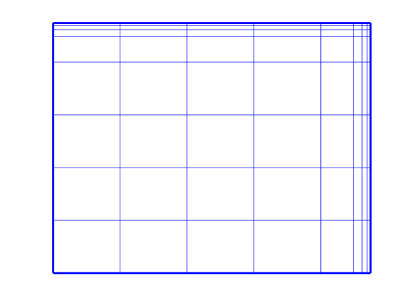
Figure 1: Bakhvalov-type mesh

Assumption 2.

In this paper, we assume that

1. $\rho\geq k+2$.

2. $\varepsilon\leq N^{-1}$.

Then we will introduce some important properties of Bakhvalov-type mesh (2).

Lemma 1.

$$C_{1}\varepsilon N^{-1}\leq h_{x,N}\leq C_{2}\varepsilon N^{-1},$$

$$h_{x,N}\leq h_{x,N-1}\leq\dots\leq h_{x,N/2+2},$$

$$1/4\rho\varepsilon\leq h_{x,N/2+2}\leq\rho\varepsilon,$$

$$1/2\rho\varepsilon\leq h_{x,N/2+1}\leq 2\rho N^{-1},$$

$$N^{-1}\leq h_{x,i}\leq 2N^{-1}\quad 1\leq i\leq N/2,$$

$$C_{3}\rho\varepsilon\ln N\leq x_{N/2+1}\leq C_{4}\rho\varepsilon\ln N,\quad x_{N/2}\geq C\varepsilon|\ln\varepsilon|.$$

Bounds for $h_{y,j}$, $1\leq j\leq N$, are analogous.

2.3 the LDG method

Define the discontinuous finite element space:

$$\mathcal{V}_{N}=\{v\in L^{2}(\Omega):\text{$v|_{K}\in\mathbb{Q}^{k}(K)$ },K\in\Omega_{N}\},$$

where $\mathbb{Q}^{k}(K)$ represents the space of tensor-product polynomials of degree $k$ in each variable on $K$. Note that the functions within the space $\mathcal{V}_{N}$ are permitted to be discontinuous at the interfaces of elements.

For $v\in\mathcal{V}_{N}$, $x\in I_{i}$ and $y\in J_{j}$, we use $v^{\pm}_{i,y}=\lim_{x\to x^{\pm}_{i}}v(x,y)$ and $v^{\pm}_{x,j}=\lim_{y\to y^{\pm}_{j}}v(x,y)$ to express the traces evaluated from the four directions. Besides, write the jumps on the vertical and horizontal edges as:

$$[[v]]_{i,y}=v^{+}_{i,y}-v^{-}_{i,y}\text{ for $i=1,2,\ldots,N-1$},\; [[v]]_{0,y}=v^{+}_{0,y},\; [[v]]_{N,y}=-v^{-}_{N,y};$$

$$[[v]]_{x,j}=v^{+}_{x,j}-v^{-}_{x,j}\text{ for $j=1,2,\ldots,N-1$},\; [[v]]_{x,0}=v^{+}_{x,0},\; [[v]]_{x,N}=-v^{-}_{x,N}.$$

Next, we present the LDG method for problem (1). Rewrite (1) by an equivalent first-order system:

$$\left\{\begin{aligned} &\varepsilon^{-1}p=u_{x}&&\quad\text{in $\Omega$},\\ &\varepsilon^{-1}q=u_{y}&&\quad\text{in $\Omega$},\\ &-p_{x}-q_{y}+a_{1}u_{x}+a_{2}u_{y}+bu=f&&\quad\text{in $\Omega$}.\end{aligned}\right.$$ (3)

For $y\in J_{j}$, $j=1,2,\ldots,N$, define the numerical fluxes by

$$\hat{P}_{i,y}=\left\{\begin{aligned} &P^{+}_{0,y}+\lambda_{1}U^{+}_{0,y}\quad&&\text{$i=0$},\\ &P^{+}_{i,y}\quad&&\text{$i=1,2,\ldots,N-1$},\\ &P^{-}_{N,y}-\lambda_{2}U^{-}_{N,y}\quad&&\text{$i=N$},\end{aligned}\right.$$

$$\hat{U}_{i,y}=\left\{\begin{aligned} &0\quad&&\text{$i=0,N$},\\ &U^{-}_{i,y}\quad&&\text{$i=1,2,\ldots,N-1$},\\ \end{aligned}\right.$$

where $0\leq\lambda_{1},\lambda_{2}\leq C$. When $x\in I_{i}$, $i=1,2,\ldots,N$, we can define $\hat{Q}_{x,j}$ and $\hat{U}_{x,j}$ for $j=1,2,\ldots,N$ analogously. Let $(\cdot,\cdot)_{D}$ be the inner product in $L^{2}(D)$ with $D\subseteq\mathbb{R}^{2}$, and $\left<\cdot,\cdot\right>_{I}$ be the inner product in $L^{2}(I)$ with $I\subseteq\mathbb{R}$. $Z=(v,s,r)\in\mathcal{V}_{N}\times\mathcal{V}_{N}\times\mathcal{V}_{N}$ $(=:\mathcal{V}_{N}^{3})$ denotes any test function. Then the compact form of the LDG method can be described as:

Find the LDG solution $W=(U,P,Q)\in\mathcal{V}_{N}^{3}$ such that

$$B(W;Z)=(f,v)\quad\forall Z=(v,s,r)\in\mathcal{V}_{N}^{3},$$

where

$$B(W;Z):=\mathcal{B}_{1}(W;Z)+\mathcal{B}_{2}(W;Z)+\mathcal{B}_{3}(W;Z)+\mathcal{B}_{4}(U;v),$$

and

$$\begin{aligned} \mathcal{B}_{1}(W;Z)=((b-\nabla\cdot\alpha)U,v)+\varepsilon^{-1}(P,s)+\varepsilon^{-1}(Q,r),\end{aligned}$$ (4)

$$\begin{aligned} \mathcal{B}_{2}(W;Z)=(U,s_{x})+\sum_{i=1}^{N-1}\sum_{j=1}^{N}\left<U^{-}_{i,y},[[s]]_{i,y}\right>_{J_{j}}+(U,r_{y})+\sum_{i=1}^{N}\sum_{j=1}^{N-1}\left<U^{-}_{x,j},[[r]]_{x,j}\right>_{I_{i}},\end{aligned}$$

$$\begin{aligned} \mathcal{B}_{3}(W;Z)=&(P,v_{x})+\sum_{j=1}^{N}\left\{\sum_{i=0}^{N-1}\left<P^{+}_{i,y},[[v]]_{i,y}\right>_{J_{j}}-\left<P^{-}_{N,y},v_{N,y}^{-}\right>_{J_{j}}\right\}\\ &+(Q,v_{y})+\sum_{i=1}^{N}\left\{\sum_{j=0}^{N-1}\left<Q^{+}_{x,j},[[v]]_{x,j}\right>_{I_{i}}-\left<Q^{-}_{x,N},v_{x,N}^{-}\right>_{I_{i}}\right\},\end{aligned}$$

$$\begin{aligned} \mathcal{B}_{4}(U;v)=&-(a_{1}U,v_{x})-\sum_{j=1}^{N}\left\{\sum_{i=1}^{N}\left<(a_{1})_{i,y}U^{-}_{i,y},[[v]]_{i,y}\right>_{J_{j}}-\left<\lambda_{1}U^{-}_{N,y},v^{-}_{N,y}\right>_{J_{j}}\right\}\\ &-(a_{2}U,v_{y})-\sum_{i=1}^{N}\left\{\sum_{j=1}^{N}\left<(a_{2})_{x,j}U^{-}_{x,j},[[v]]_{x,j}\right>_{I_{i}}-\left<\lambda_{2}U^{-}_{x,N},v^{-}_{x,N}\right>_{I_{i}}\right\}.\end{aligned}$$

Let $w=(u,p,q)$ be the exact solution of (3). According to (4), we can define the energy norm as

$$|||w|||_{E}^{2}=B(w;w)= |||w|||_{2}^{2}+\sum_{j=1}^{N}\left\{\sum_{i=0}^{N-1}\frac{1}{2}\left<(a_{1})_{i,y},[[u]]^{2}_{i,y}\right>_{J_{j}}+\left<\frac{1}{2}(a_{1})_{N,y}+\lambda_{1},[[u]]^{2}_{N,y}\right>_{J_{j}}\right\}$$ (5)

$$+\sum_{i=1}^{N}\left\{\sum_{j=0}^{N-1}\frac{1}{2}\left<(a_{2})_{x,j},[[u]]^{2}_{x,j}\right>_{I_{i}}+\left<\frac{1}{2}(a_{2})_{x,N}+\lambda_{2},[[u]]^{2}_{x,N}\right>_{I_{i}}\right\},$$

where $|||w|||_{2}^{2}=:\varepsilon^{-1}||p||^{2}+\varepsilon^{-1}||q||^{2}+||(b-\frac{1}{2}\nabla\cdot\boldsymbol{\alpha})^{\frac{1}{2}}u||^{2}$.

3 Local Gauss-Radau projections, new interpolation and some preliminary results

3.1 Local Gauss-Radau projections

In this part, we will design several two-dimensional local Gauss-Radau projections. For each $K_{ij}\in\Omega_{N}$, set $\mathcal{Q}^{k}(K_{ij}):=\mathcal{P}^{k}(I_{i})\otimes\mathcal{P}^{k}(J_{j})$, where $\mathcal{P}^{k}(I_{i})$ represents the set of polynomials with degree $k$ defined on any one-dimensional interval $I_{i}$. $\forall z\in C(\overline{K}_{ij})$, we define the local Gauss-Radau projections $\pi-$, $\pi^{-}_{x}$, $\pi^{-}_{y}$, $\pi^{+}_{x}$, $\pi^{+}_{y}\in\mathcal{Q}^{k}(K_{ij})$ with $i,j=1,\cdots,N$ as:

$$\left\{\begin{aligned} &(\pi^{-}z,v)_{K_{ij}}=(z,v)_{K_{ij}}\quad&&\text{$\forall v\in\mathcal{Q}^{k-1}(K_{ij})$},\\ &\left<(\pi^{-}z)^{-}_{i,y},v\right>_{J_{j}}=\left<z^{-}_{i,y},v\right>_{J_{j}}\quad&&\forall v\in\mathcal{P}^{k-1}(J_{j}),\\ &\left<(\pi^{-}z)^{-}_{x,j},v\right>_{I_{i}}=\left<z^{-}_{x,j},v\right>_{I_{i}}\quad&&\forall v\in\mathcal{P}^{k-1}(I_{i}),\\ &(\pi^{-}z)(x_{i}^{-},y_{j}^{-})=z(x_{i}^{-},y_{j}^{-}),\end{aligned}\right.$$

$$\left\{\begin{aligned} &(\pi^{-}_{x}z,v)_{K_{ij}}=(z,v)_{K_{ij}}\quad&&\text{$\forall v\in\mathcal{P}^{k-1}(I_{i})\otimes\mathcal{P}^{k}(J_{j})$},\\ &\left<(\pi^{-}_{x}z)^{-}_{i,y},v\right>_{J_{j}}=\left<z^{-}_{i,y},v\right>_{J_{j}}\quad&&\forall v\in\mathcal{P}^{k}(J_{j}),\end{aligned}\right.$$

$$\left\{\begin{aligned} &(\pi^{-}_{y}z,v)_{K_{ij}}=(z,v)_{K_{ij}}\quad&&\text{$\forall v\in\mathcal{P}^{k}(I_{i})\otimes\mathcal{P}^{k-1}(J_{j})$},\\ &\left<(\pi^{-}_{y}z)^{-}_{x,j},v\right>_{I_{i}}=\left<z^{-}_{x,j},v\right>_{I_{i}}\quad&&\forall v\in\mathcal{P}^{k}(I_{i}),\end{aligned}\right.$$

$$\left\{\begin{aligned} &(\pi^{+}_{x}z,v)_{K_{ij}}=(z,v)_{K_{ij}}\quad&&\text{$\forall v\in\mathcal{P}^{k-1}(I_{i})\otimes\mathcal{P}^{k}(J_{j})$},\\ &\left<(\pi^{+}_{x}z)^{+}_{i,y},v\right>_{J_{j}}=\left<z^{+}_{i,y},v\right>_{J_{j}}\quad&&\forall v\in\mathcal{P}^{k}(J_{j}),\end{aligned}\right.$$

$$\left\{\begin{aligned} &(\pi^{+}_{y}z,v)_{K_{ij}}=(z,v)_{K_{ij}}\quad&&\text{$\forall v\in\mathcal{P}^{k}(I_{i})\otimes\mathcal{P}^{k-1}(J_{j})$},\\ &\left<(\pi^{+}_{y}z)^{+}_{x,j},v\right>_{I_{i}}=\left<z^{+}_{x,j},v\right>_{I_{i}}\quad&&\forall v\in\mathcal{P}^{k}(I_{i}).\end{aligned}\right.$$

It can be deduced that $\pi^{-},\pi^{-}_{x},\pi^{-}_{y},\pi^{+}_{x},\pi^{+}_{y}$ exist and are unique under these conditions [17]. Moreover, the projections $\Pi\in\left\{\pi^{-},\pi_{x}^{-},\pi_{y}^{-},\pi_{x}^{+},\pi_{y}^{+}\right\}$ possess the following stability properties and approximation properties as stated in [16, Lemma 2.14]:

$$\|\Pi z\|_{L^{\infty}(K_{ij})}\leq C\|z\|_{L^{\infty}(K_{ij})},$$

$$\|z-\Pi z\|_{K_{ij}}\leq C\left[h_{x,i}^{k+1}\|\partial_{x}^{k+1}z\|_{K_{ij}}+h_{y,j}^{k+1}\|\partial_{y}^{k+1}z\|_{K_{ij}}\right].$$

3.2 New interpolation

Then, establish the new interpolation $\pi w=(\mathcal{P}^{-}u,\mathcal{P}_{x}^{+}p,\mathcal{P}_{y}^{+}q)$ of the true solution $w=(u,p,q)$, where $\mathcal{P}^{-}u,\mathcal{P}_{x}^{+}p$ and $\mathcal{P}_{y}^{+}q$ are defined as:

$$\mathcal{P}^{-}u=\left\{\begin{aligned} &\pi^{-}_{x}u\quad(x,y)\in[x_{N/2-1},x_{N/2}]\times([0,y_{N/2-1}]\cup[y_{N/2},1]),\\ &\pi^{-}_{y}u\quad(x,y)\in[y_{N/2-1},y_{N/2}]\times([0,x_{N/2-1}]\cup[x_{N/2},1]),\\ &\pi^{-}u\quad(x,y)\in{\text{o}therwise},\end{aligned}\right.$$ (6)

$$\mathcal{P}^{+}_{x}p=\begin{aligned} \pi^{+}_{x}p\quad(x,y)\in\Omega,\\ \end{aligned}$$

$$\mathcal{P}^{+}_{y}q=\begin{aligned} \pi^{+}_{y}q\quad(x,y)\in\Omega.\\ \end{aligned}$$

Remark 1.

The supercloseness result estimated by the previously defined local Gauss-Radau projections $\pi^{-}$, $\pi_{x}^{+}$, $\pi_{y}^{+}$ and interpolation $(\pi^{-}u,\pi_{x}^{+}p,\pi_{y}^{+}q)$ (see [2] and [4]) was affected by the factor $(\ln(1/\varepsilon))^{1/2}$. Here, we newly introduce two special local Gauss-Radau projections $\pi_{x}^{-}$ and $\pi_{y}^{-}$, and construct a new interpolation $(\mathcal{P}^{-}u,\pi_{x}^{+}p,\pi_{y}^{+}q)$ to further eliminate some intractable element errors. Utilizing this new interpolation, we succeed in eliminating the factor $(\ln(1/\varepsilon))^{1/2}$ and demonstrating parameter-uniform supercloseness of an optimal order $k+1$ in the following analysis.

3.3 Preliminary results

In this part, we will introduce some preliminary conclusions.

Define

$$\eta=w-\pi w=(\eta_{u},\eta_{p},\eta_{q})=(u-P^{-}u,p-P^{+}_{x}p,q-P^{+}_{y}q),$$

$$\xi=W-\pi w=(\xi_{u},\xi_{p},\xi_{q})=(U-P^{-}u,P-P^{+}_{x}p,Q-P^{+}_{y}q),$$

where $w$ is the exact solution of (3), $\pi w$ is the interpolation of $w$, and $W$ is the LDG solution. Then, the error $e=(u-U,p-P,q-Q)$ can be represented as

$$e=w-W=\eta-\xi.$$

In the following lemma, we will showcase some interpolation error estimates. Note that $\|\cdot\|_{L^{n}(D)}$ represents norms in the Lebesgue space. When $n=2$, $\|\cdot\|_{L^{2}(\Omega)}$ is written as $\|\cdot\|$ for simplicity.

Lemma 2.

For $i,j=1,\dots,N$, there exists $C$ such that

$$\|\eta_{u}\|_{L^{\infty}(\Omega)}\leq CN^{-(k+1)},$$

$$\|(\eta_{u})_{i,y}^{-}\|_{L^{\infty}(K_{ij})}+\|(\eta_{u})_{x,j}^{-}\|_{L^{\infty}(K_{ij})}\leq CN^{-(k+1)},$$

$$\|(\eta_{u})_{i,y}^{-}\|_{J_{j}}+\|(\eta_{u})_{x,j}^{-}\|_{I_{i}}\leq CN^{-(k+3/2)},$$

$$\sum_{j=1}^{N}\|(\eta_{u})_{i,y}^{-}\|_{J_{j}}^{2}+\sum_{i=1}^{N}\|(\eta_{u})_{x,j}^{-}\|_{I_{i}}^{2}\leq CN^{-2(k+1)},$$

$$\varepsilon^{-1/2}\|\eta_{p}\|+\varepsilon^{-1/2}\|\eta_{q}\|\leq CN^{-(k+1)}.$$

Proof.

The aforementioned estimates can be analogously derived by consulting [2, Lemma 4.1], which provides comparable methods and results. ∎

Next, we will present a lemma proposed in [4, Lemma 3.3] to bound $\xi$.

Lemma 3.

There exists a constant $C$ such that

$$\|(\xi_{u})_{x}\|_{[x_{N/2},1]\cup[0,1]}+\left(\sum_{i=N/2+1}^{N}\sum_{j=1}^{N}h_{x,i}^{-1}\|[[\xi_{u}]]_{i-1,y}\|_{J_{j}}^{2}\right)^{1/2}\leq C\varepsilon^{-1/2}\left[|||\xi|||_{E}+N^{-(k+1)}\right],$$

$$\|(\xi_{u})_{x}\|_{[0,1]\cup[y_{N/2},1]}+\left(\sum_{i=1}^{N}\sum_{j=N/2+1}^{N}h_{y,j}^{-1}\|[[\xi_{u}]]_{x,j-1}\|_{I_{i}}^{2}\right)^{1/2}\leq C\varepsilon^{-1/2}\left[|||\xi|||_{E}+N^{-(k+1)}\right].$$

4 Supercloseness analysis

Owing to the consistency of numerical fluxes and the smooth assumptions of $u$, $p$ and $q$, one can obtain

$$B(\xi;Z)=B(\eta;Z)\quad\forall Z\in\mathcal{V}_{N}^{3}.$$ (7)

Set $Z=\xi$ in (7), in light of the definition of $|||\cdot|||_{E}$ and the Galerkin orthogonality, we can derive

$$|||\xi|||_{E}^{2}=B(\xi;\xi)=B(\eta;\xi):=\sum_{i=1}^{3}\mathcal{B}_{i}(\eta;\xi)+\mathcal{B}_{4}(\eta_{u};\xi_{u}),$$ (8)

here $\mathcal{B}_{i}(i=1,2,3,4)$ can be expressed in accordance with (4).

Refer to [4, Theorem 4.1], we can further rewrite the $x$-direction component of $\mathcal{B}_{4}(\eta_{u};\xi_{u})$ into the following form:

$$\mathcal{B}_{4}^{x}(\eta_{u};\xi_{u})= -(a_{1}\eta_{u},(\xi_{u})_{x})-\sum_{j=1}^{N}\left\{\sum_{i=1}^{N}\left<(a_{1})_{i,y}(\eta_{u})^{-}_{i,y},[[\xi_{u}]]_{i,y}\right>_{J_{j}}-\left<\lambda_{1}(\eta_{u})^{-}_{N,y},(\xi_{u})^{-}_{N,y}\right>_{J_{j}}\right\}$$

$$:= \sum_{i=1}^{5}\mathcal{B}_{4i}^{x}(\eta_{u};\xi_{u}),$$

where

$$\begin{aligned} \mathcal{B}_{41}^{x}(\eta_{u};\xi_{u})=-\sum_{i=1}^{N/2}\sum_{j=1}^{N}(a_{1})_{ij}\mathcal{D}_{ij}^{1}(\eta_{u},\xi_{u}),\end{aligned}$$

$$\begin{aligned} \mathcal{B}_{42}^{x}(\eta_{u};\xi_{u})=&-\sum_{i=1}^{N/2}\sum_{j=1}^{N}\left[\left<(a_{1}-(a_{1})_{ij})\eta_{u},(\xi_{u})_{x}\right>_{K_{ij}}+\left<((a_{1})_{i-1,y}-(a_{1})_{ij})(\eta_{u})_{i-1,y}^{-},(\xi_{u})_{i-1,y}^{+}\right>_{J_{j}}\right.\\ &\left.-\left<((a_{1})_{i,y}-(a_{1})_{ij})(\eta_{u})_{i,y}^{-},(\xi_{u})_{i,y}^{-}\right>_{J_{j}}\right],\end{aligned}$$

$$\begin{aligned} \mathcal{B}_{43}^{x}(\eta_{u};\xi_{u})=-\sum_{i=N/2+1}^{N}\sum_{j=1}^{N}\left<a_{1}\eta_{u},(\xi_{u})_{x}\right>_{K_{ij}}-\sum_{i=N/2+1}^{N}\sum_{j=1}^{N}\left<(a_{1})_{i,y}(\eta_{u})_{i,y}^{-},[[\xi_{u}]]_{i,y}\right>_{J_{j}},\end{aligned}$$

$$\begin{aligned} \mathcal{B}_{44}^{x}(\eta_{u};\xi_{u})=-\sum_{j=1}^{N}(a_{1})_{N/2,y}\left<(\eta_{u})_{N/2,y}^{-},(\xi_{u})_{N/2,y}^{+}\right>_{J_{j}},\end{aligned}$$

$$\begin{aligned} \mathcal{B}_{45}^{x}(\eta_{u};\xi_{u})=\sum_{j=1}^{N}\lambda_{1}\left<(\eta_{u})_{N,y}^{-},(\xi_{u})_{N,y}^{-}\right>_{J_{j}}.\end{aligned}$$

Here $(a_{1})_{ij}$ denotes $a_{1}(x_{i},y_{j})$ and $\mathcal{D}_{ij}^{1}(\eta_{u},\xi_{u}):=\left<\eta_{u},(\xi_{u})_{x}\right>_{K_{ij}}-\left<(\eta_{u})_{i,y}^{-},(\xi_{u})_{i,y}^{-}\right>_{J_{j}}+\left<(\eta_{u})_{i-1,y}^{-},(\xi_{u})_{i-1,y}^{+}\right>_{J_{j}}$. In the following analysis, we will just analyze $\mathcal{B}_{4}^{x}(\eta_{u};\xi_{u})$, for $\mathcal{B}_{4}^{y}(\eta_{u};\xi_{u})$ (the $y$-direction component of $\mathcal{B}_{4}(\eta_{u};\xi_{u})$) can be analyzed similarly.

The estimate approach for $\mathcal{B}_{i}(\eta;\xi)\ i=1,2,3$ is akin to the one in [2, Theorem 4.1], and the proof for $\mathcal{B}_{4i}^{x}(\eta_{u};\xi_{u})\ i=1,2,5$ closely resembles that in [4, Theorem 4.1]. Consequently, we can easily derive that

$$|\mathcal{B}_{i}(\eta;\xi)|\leq CN^{-(k+1)}|||\xi|||_{E}\quad i=1,2,3,$$ (9)

and

$$|\mathcal{B}_{4i}^{x}(\eta_{u};\xi_{u})|\leq CN^{-(k+1)}|||\xi|||_{E}\quad i=1,2,5.$$ (10)

For $\mathcal{B}_{43}^{x}(\eta_{u};\xi_{u})$, its supercloseness result was $\mathcal{O}(N^{-(k+1)}\ln(1/\varepsilon)^{1/2})$ in the analysis of [4]. To eliminate $(\ln(1/\varepsilon))^{1/2}$, we attempt to improve the analysis technique proposed in [4, Lemma 3.3] by considering the situation on the interval $[x_{N/2},x_{N/2+1}]$ and $[x_{N/2+1},x_{N}]$ separately, which can effectively avoid the influence of the layer width $\mathcal{O}(\varepsilon\ln(1/\varepsilon))$. As a result of this enhancement, we successfully attain the optimal convergence rate independent of $\varepsilon$, see Lemma 4.

And for $\mathcal{B}_{44}^{x}(\eta_{u};\xi_{u})$, previous methods were unable to avoid $(\ln(1/\varepsilon))^{1/2}$. In this article, we newly introduce two special local Gauss-Radau projections $\pi_{x}^{-}$, $\pi_{y}^{-}$, and establish a new interpolation $(\mathcal{P}^{-}u,\mathcal{P}_{x}^{+}p,\mathcal{P}_{u}^{+}q)$ to further eliminate element boundary errors on the region $[x_{N/2-1},x_{N/2}]\times([0,y_{N/2-1}]\cup[y_{N/2},1])$. Then concentrating the analysis on a specific mesh $K_{N/2,N/2}$, where an optimal supercloseness result independent of $\varepsilon$ can be achieved through the utilization of a skillful technique, as demonstrated in Lemma 5.

Lemma 4.

$$|\mathcal{B}_{43}^{x}(\eta_{u};\xi_{u})|\leq CN^{-(k+1)}\ln^{1/2}N(|||\xi|||_{E}+N^{-(k+1)}).$$

Proof.

$$\mathcal{B}_{43}^{x}(\eta_{u};\xi_{u})= -\sum_{j=1}^{N}\left<a_{1}\eta_{u},(\xi_{u})_{x}\right>_{K_{N/2+1,j}}-\sum_{j=1}^{N}\left<(a_{1})_{N/2+1,y}(\eta_{u})_{N/2+1,y}^{-},[[\xi_{u}]]_{N/2+1,y}\right>_{J_{j}}$$ (11)

$$-\sum_{i=N/2+2}^{N}\sum_{j=1}^{N}\left<a_{1}\eta_{u},(\xi_{u})_{x}\right>_{K_{ij}}-\sum_{i=N/2+2}^{N}\sum_{j=1}^{N}\left<(a_{1})_{i,y}(\eta_{u})_{i,y}^{-},[[\xi_{u}]]_{i,y}\right>_{J_{j}}$$

$$= I+II+III+IV.$$

Recall Hölder inequalities, Lemma 2 and inverse inequality, we have

$$|I|\leq C\sum_{j=1}^{N}\|(\eta_{u})\|_{K_{N/2+1,j}}\|(\xi_{u})_{x}\|_{K_{N/2+1,j}}$$ (12)

$$\leq C\sum_{j=1}^{N}N^{-(k+1)}h_{x,N/2+1}^{1/2}h_{y,j}^{1/2}h_{x,N/2+1}^{-1/2}\|\xi_{u}\|_{K_{N/2+1,j}}$$

$$\leq CN^{-(k+1)}|||\xi|||_{E}.$$

Hölder inequalities, Lemma 2 and (5) give

$$|II|\leq(\sum_{j=1}^{N}\|(\eta_{u})_{N/2+1,y}^{-}\|_{J_{j}}^{2})^{1/2}(\sum_{j=1}^{N}\|[[\xi_{u}]]_{N/2+1,y}\|_{J_{j}}^{2})^{1/2}\leq CN^{-(k+1)}|||\xi|||_{E}.$$ (13)

Hölder inequalities, (5), Lemmas 1, 2 and 3 yield

$$|III+IV|\leq C\|\eta_{u}\|_{[x_{N/2+1},1]\cup[0,1]}\|(\xi_{u})_{x}\|_{[x_{N/2+1},1]\cup[0,1]}$$ (14)

$$+C\left(\sum_{i=N/2+2}^{N-1}\sum_{j=1}^{N}h_{x,i+1}\|(\eta_{u})_{i,y}^{-}\|_{J_{j}}^{2}\right)^{1/2}\left(\sum_{i=N/2+2}^{N-1}\sum_{j=1}^{N}h_{x,i+1}^{-1}\|[[\xi_{u}]]_{i,y}\|_{J_{j}}^{2}\right)^{1/2}$$

$$+C\left(\sum_{j=1}^{N}\|(\eta_{u})_{N,y}^{-}\|_{J_{j}}^{2}\right)^{1/2}\left(\sum_{j=1}^{N}\|[[\xi_{u}]]_{N,y}\|_{J_{j}}^{2}\right)^{1/2}$$

$$\leq C\left(\|\eta_{u}\|_{[x_{N/2+1},1]\cup[0,1]}^{2}+\sum_{i=N/2+2}^{N-1}\sum_{j=1}^{N}h_{x,i+1}\|(\eta_{u})_{i,y}^{-}\|_{J_{j}}^{2}\right)^{1/2}$$

$$\cdot\left(\|(\xi_{u})_{x}\|_{[x_{N/2+1},1]\cup[0,1]}^{2}+\sum_{i=N/2+2}^{N-1}\sum_{j=1}^{N}h_{x,i+1}^{-1}\|[[\xi_{u}]]_{i,y}\|_{J_{j}}^{2}\right)^{1/2}+CN^{-(k+1)}|||\xi|||_{E}$$

$$\leq C\varepsilon^{-1/2}\left(\|\eta_{u}\|_{[x_{N/2+1},1]\cup[0,1]}^{2}+\sum_{i=N/2+2}^{N-1}\sum_{j=1}^{N}h_{x,i+1}\|(\eta_{u})_{i,y}^{-}\|_{J_{j}}^{2}\right)^{1/2}(|||\xi|||_{E}+N^{-(k+1)})$$

$$+CN^{-(k+1)}|||\xi|||_{E}$$

$$\leq CN^{-(k+1)}\ln^{1/2}N(|||\xi|||_{E}+N^{-(k+1)}).$$

Substitute (12), (13) and (14) into (11), we can prove Lemma 4. ∎

Lemma 5.

$$|\mathcal{B}_{44}^{x}(\eta_{u};\xi_{u})|\leq CN^{-(k+1)}|||\xi|||_{E}.$$

Proof.

Consider the novel interpolation (6) and the local Gauss-Radau projections $\pi^{-}$, $\pi_{x}^{-}$, one has

$$\mathcal{B}_{44}^{x}(\eta_{u};\xi_{u})= -\sum_{j=1}^{N}(a_{1})_{N/2,y}\left<(\eta_{u})_{N/2,y}^{-},(\xi_{u})_{N/2,y}^{+}\right>_{J_{j}}$$

$$= -(\sum_{j=1}^{N/2-1}+\sum_{j=N/2+1}^{N})(a_{1})_{N/2,y}\left<(\eta_{u})_{N/2,y}^{-},(\xi_{u})_{N/2,y}^{+}\right>_{J_{j}}$$

$$-(a_{1})_{N/2,y}\left<(\eta_{u})_{N/2,y}^{-},(\xi_{u})_{N/2,y}^{+}\right>_{J_{N/2}}$$

$$= -(a_{1})_{N/2,y}\left<(\eta_{u})_{N/2,y}^{-},(\xi_{u})_{N/2,y}^{+}\right>_{J_{N/2}}.$$

To get an accurate estimate for $-(a_{1})_{N/2,y}\left<(\eta_{u})_{N/2,y}^{-},(\xi_{u})_{N/2,y}^{+}\right>_{J_{N/2}}$, we adopt a skillful technique by decomposing it into the following two terms:

$$-(a_{1})_{N/2,y}\left<(\eta_{u})_{N/2,y}^{-},(\xi_{u})_{N/2,y}^{+}\right>_{J_{N/2}}$$

$$= -(a_{1})_{N/2,y}\left<(\eta_{u})_{N/2,y}^{-},[[\xi_{u}]]_{N/2,y}\right>_{J_{N/2}}-(a_{1})_{N/2,y}\left<(\eta_{u})_{N/2,y}^{-},(\xi_{u})_{N/2,y}^{-}\right>_{J_{N/2}},$$

where from Hölder inequalities, Lemma 2 and (5), we can derive

$$|-(a_{1})_{N/2,y}\left<(\eta_{u})_{N/2,y}^{-},[[\xi_{u}]]_{N/2,y}\right>_{J_{N/2}}|\leq CN^{-(k+3/2)}|||\xi|||_{E},$$

and by Hölder inequalities, Lemma 2, trace inequality and (5), one can obtain

$$|-(a_{1})_{N/2,y}\left<(\eta_{u})_{N/2,y}^{-},(\xi_{u})_{N/2,y}^{-}\right>_{J_{N/2}}|\leq CN^{-(k+3/2)}N^{1/2}\|\xi_{u}\|_{K_{N/2,N/2}}$$

$$\leq CN^{-(k+1)}|||\xi|||_{E}.$$

Thus we have proven Lemma 5. ∎

At this point, we will present the main conclusion of this paper.

Theorem 1.

Let $w=(u,p,q)=(u,\varepsilon u_{x},\varepsilon u_{y})$, where $u$ is the exact solution of problem (1). Define the interpolation of $w$ as $\pi w=(P^{-}u,P_{x}^{+}p,P_{y}^{+}q)\in\mathcal{V}_{N}^{3}$, and the LDG solution as $W=(U,P,Q)\in\mathcal{V}_{N}^{3}$. Then we can establish the following supercloseness result:

$$|||\pi w-W|||_{E}\leq CN^{-(k+1)}\ln^{1/2}N.$$

Proof.

According to (10), Lemmas 4 and 5, one has

$$|\mathcal{B}_{4}^{x}(\eta_{u};\xi_{u})|\leq CN^{-(k+1)}\ln^{1/2}N(|||\xi|||_{E}+N^{-(k+1)}).$$

We can estimate $\mathcal{B}_{4}^{y}(\eta_{u};\xi_{u})$ analogously and consequently, one obtains

$$|\mathcal{B}_{4}(\eta_{u};\xi_{u})|\leq CN^{-(k+1)}\ln^{1/2}N(|||\xi|||_{E}+N^{-(k+1)}).$$ (15)

(15), combined with (9) gives

$$|||\xi|||_{E}^{2}=B(\eta;\xi)=\sum_{i=1}^{3}\mathcal{B}_{i}(\eta;\xi)+\mathcal{B}_{4}(\eta_{u};\xi_{u})\leq CN^{-(k+1)}\ln^{1/2}N(|||\xi|||_{E}+N^{-(k+1)}),$$

i.e.

$$|||\xi|||_{E}=|||\pi w-W|||_{E}\leq CN^{-(k+1)}\ln^{1/2}N.$$

Thus we have done. ∎

Remark 2.

With further derivation, we can obtain the $L^{2}$ error estimate:

$$|||w-W|||_{2}\leq CN^{-(k+1)}\ln^{1/2}N.$$

Proof.

Triangle inequality yields

$$|||w-W|||_{2}=|||\eta-\xi|||_{2}\leq|||\eta|||_{2}+|||\xi|||_{2},$$

where from (5) and Lemma 2, one can get

$$|||\eta|||_{2}\leq C(\|\eta_{u}\|+\varepsilon^{-1/2}\|\eta_{p}\|+\varepsilon^{-1/2}\|\eta_{q}\|)\leq CN^{-(k+1)},$$

and from (5) and Theorem 1, one has

$$|||\xi|||_{2}\leq|||\xi|||_{E}\leq CN^{-(k+1)}\ln^{1/2}N.$$

∎

Remark 3.

The primary emphasis of this article is on the level of numerical analysis, while the corresponding algorithm is consistent with the one employed in [4] for Bakhvalov-type mesh. Hence, we omit numerical experiments in this article, and recommend consulting [4, Section 5] for relevant numerical experiments, which can also support our main conclusion, i.e., Theorem 1.

5 Conflict of interest statement

We declare that we have no conflict of interest.

References

- [1] H. Zhu, and Z. Zhang. Uniform convergence of the LDG method for a singularly perturbed problem with the exponential boundary layer. Math. Comput., 83:635–663, 2013.
- [2] Y. Cheng, Y. Mei, and H-G. Roos. The local discontinuous Galerkin method on layer-adapted meshes for time-dependent singularly perturbed convection-diffusion problems. Comput. Math. Appl., 117:245–256, 2022.
- [3] Y. Cheng and Y. Mei. Analysis of generalised alternating local discontinuous Galerkin method on layer-adapted mesh for singularly perturbed problems. Calcolo, 58(4):Paper No. 52, 36, 2021.
- [4] Y. Cheng, S. Jiang, and M. Stynes. Supercloseness of the local discontinuous Galerkin method for a singularly perturbed convection-diffusion problem. Math. Comput., 2023.
- [5] B. Cockburn and C. Shu. The local discontinuous Galerkin method for time-dependent convection-diffusion systems. SIAM J. Numer. Anal., 35(6):2440–2463, 1998.
- [6] T. Linß. Layer-adapted Meshes for Reaction-convection-diffusion Problems. Springer-Verlag, Berlin, 2010.
- [7] Y. Mei, Y. Cheng, S. Wang, and Z. Xu. Local discontinuous galerkin method on layer-adapted meshes for singularly perturbed reaction-diffusion problems in two dimensions. arXiv preprint, 2021.
- [8] J. J. H. Miller, E. O’Riordan, and G. I. Shishkin. Fitted Numerical Methods for Singular Perturbation Problems. World Scientific, Hackensack, 2012.
- [9] H-G. Roos. Error estimates for linear finite elements on Bakhvalov-type meshes. Appl. Math., 51(1):63–72, 2006.
- [10] H-G. Roos, M. Stynes, and L. Tobiska. Robust Numerical Methods for Singularly Perturbed Differential Equations. Springer Science, Business Media, 2008.
- [11] Z. Xie and Z. Zhang. Uniform superconvergence analysis of the discontinuous Galerkin method for a singularly perturbed problem in 1-D. Math. Comp., 79(269):35–45, 2010.
- [12] Z. Xie, Z. Zhang, and Z. Zhang. A numerical study of uniform superconvergence of LDG method for solving singularly perturbed problems. J. Comput. Math., 27(2-3):280–298, 2009.
- [13] Y. Xu and C. Shu. Local discontinuous Galerkin methods for high-order time-dependent partial differential equations. Commun. Comput. Phys., 7(1):1–46, 2010.
- [14] H. Zhu and F. Celiker. Nodal superconvergence of the local discontinuous Galerkin method for singularly perturbed problems. J. Comput. Appl. Math., 330:95–116, 2018.
- [15] H. Zhu and Z. Zhang. Uniform convergence of the LDG method for a singularly perturbed problem with the exponential boundary layer. Math. Comp., 83(286):635–663, 2014.
- [16] T. Apel. Anisotropic Finite Elements: Local Estimates and Applications. Advances in Numerical Mathematics, Stuttgart, 1999.
- [17] P. Castillo, B. Cockburn, D. Schötzau, and C. Schwab. Optimal a priori error estimates for the hp-version of the local discontinuous Galerkin method for convection-diffusion problems. Math. Comp., 71(238):455–478, 2002.
- [18] S. Xie, H. Tu, and P. Zhu. Supercloseness result of higher order FEM/LDG coupled method for solving singularly perturbed problem on S-yype mesh. Abstr. Appl. Anal., Pages Art. ID 260840 11, 2014.
- [19] H.-G. Roos. Error estimates for linear finite elements on Bakhvalov-type meshes. Appl. Math., 51:63-72, 2006.
- [20] J. Zhang and X. Liu. Optimal order of uniform convergence for finite element method on Bakhvalov-type meshes. J. Sci. Comput., 85(1):2, 2020.
- [21] H.-G. Roos and M. Stynes. Some open questions in the numerical analysis of singularly perturbed differential equations. Comput. Methods Appl. Math., 15(4):531–550, 2015.
- [22] J. Zhang and X. Liu. Supercloseness and postprocessing for linear finite element method on Bakhvalov-type meshes. Numer. Algorithms, 92(3):1553–1570, 2023.