Seq-HGNN: Learning Sequential Node Representation
on Heterogeneous Graph

Abstract.

Recent years have witnessed the rapid development of heterogeneous graph neural networks (HGNNs) in information retrieval (IR) applications. Many existing HGNNs design a variety of tailor-made graph convolutions to capture structural and semantic information in heterogeneous graphs. However, existing HGNNs usually represent each node as a single vector in the multi-layer graph convolution calculation, which makes the high-level graph convolution layer fail to distinguish information from different relations and different orders, resulting in the information loss in the message passing. To this end, we propose a novel heterogeneous graph neural network with sequential node representation, namely Seq-HGNN. To avoid the information loss caused by the single vector node representation, we first design a sequential node representation learning mechanism to represent each node as a sequence of meta-path representations during the node message passing. Then we propose a heterogeneous representation fusion module, empowering Seq-HGNN  to identify important meta-paths and aggregate their representations into a compact one. We conduct extensive experiments on four widely used datasets from Heterogeneous Graph Benchmark (HGB) and Open Graph Benchmark (OGB). Experimental results show that our proposed method outperforms state-of-the-art baselines in both accuracy and efficiency. The source code is available at https://github.com/nobrowning/SEQ_HGNN.

1. Introduction

Heterogeneous graph-structured data widely exists in the real world, such as social networks, academic networks, user interaction networks, etc. In order to take advantage of the rich structural and semantic information in heterogeneous graphs, heterogeneous graph neural networks (HGNNs) have been increasingly used in information retrieval (IR) applications, ranging from search engines (Guan et al., 2022; Chen et al., 2022; Yang, 2020) and recommendation systems (Cai et al., 2022; Song et al., 2022; Pang et al., 2022) to question answering systems (Feng et al., 2022; Gao et al., 2022).

HGNNs can integrate structural and semantic information in heterogeneous graphs into node representations to meet downstream tasks. Existing HGNNs (Schlichtkrull et al., 2018; Hu et al., 2020a; Yu et al., 2022) usually deploy multiple layers of graph convolution (i.e., message passing) to capture the neighborhood information of low-order and high-order neighbors in a graph. For a particular node, each layer of convolutions represents it as one single vector, which is the input of the next higher layer. Consequently, the single vector incorporates mixed neighbor information from different relationships and distinct orders. That is, higher-level convolutions are incapable of distinguishing messages from various sources by a single vector which leads to structural information loss and difficulty in refining message passing strategy. Here we take a classic graph learning for instance, as shown in Figure 1, a sampled sub-graph contains target node $t$, two source nodes ($s_{1}$ and $s_{2}$) and two 2-hop source nodes ($ss_{1}$ and $ss_{2}$). The $ss_{1}$ and $ss_{2}$ are the source node of ($s_{1}$ and $s_{2}$), respectively.

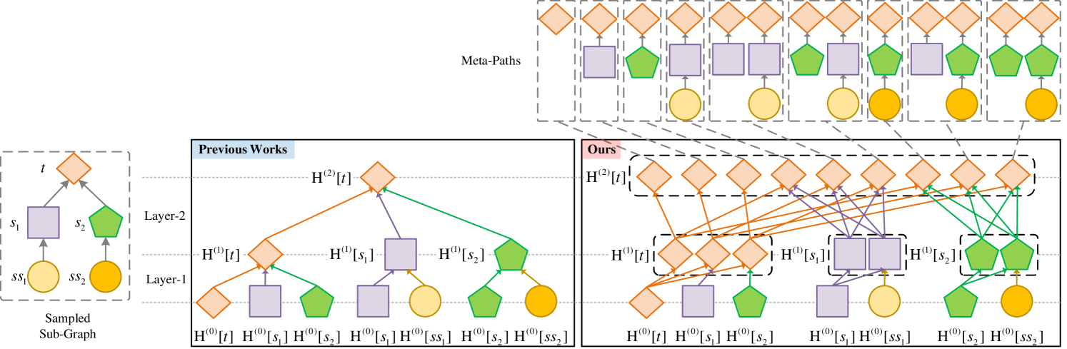
Figure 1. The comparison of node representation updates. The shapes of the nodes represent different node types.

The comparison of node representation updates. The shapes of the nodes represent different node types.

Existing methods (Schlichtkrull et al., 2018; Hu et al., 2020a; Yu et al., 2022) usually conduct graph convolution operations twice to learn the node representation. Through the first layer of graph convolution, the target node $t$ and its neighbors (source nodes) are represented as $\mathbf{H}^{(1)}[t]$, $\mathbf{H}^{(1)}[s_{1}]$, and $\mathbf{H}^{(1)}[s_{2}]$, respectively, which are used as the input of the next layer of graph convolution computation. The information in $s_{1}$ and $ss_{1}$ is mixed in $\mathbf{H}^{(1)}[s_{1}]$ and information of $s_{2}$ and $ss_{2}$ is mixed in $\mathbf{H}^{(1)}[s_{2}]$. Based on the $\mathbf{H}^{(1)}[t]$, $\mathbf{H}^{(1)}[s_{1}]$, and $\mathbf{H}^{(1)}[s_{2}]$, the second layer of graph convolution cannot distinguish the information from $ss_{1}$ and $s_{1}$ and the information from $ss_{2}$ and $s_{2}$.

Intuitively, the semantics learned from each layer and each relation can reflect different-grained features, which strongly correlate to the different tasks, while the mixtures of all information may lead to sub-optimal results for the downstream tasks.

Along this line, we propose a novel heterogeneous graph neural network with sequential node representation (Seq-HGNN), which learns representations of meta-paths and fuses them into high-quality node representations. Specifically, we first propose a sequential node representation learning mechanism that performs message passing over all meta-paths within fixed hops and represents each node as a sequence of meta-path representation. As Figure 1 illustrates, after the calculation of two Seq-HGNN  layers, Seq-HGNN  can automatically capture the information of all meta-paths and their combinations within 2 hops, which are respectively stored in multiple independent vectors. These vectors then form a sequence as the representation of target $t$ (i.e. $\mathbf{H}^{(2)}[t]$). The sequential representation enables higher Seq-HGNN  layers to naturally distinguish messages from different meta-paths. Secondly, we design a heterogeneous representation fusion module to transform the sequence-based node representations into a compact representation, which can be used in various downstream tasks. Also, Seq-HGNN  can benefit the discovery of effective entities and relations by estimating the importance of different meta-paths. Finally, we conduct extensive experiments on real-world datasets. The experimental results show that Seq-HGNN  achieves the best performance compared with several state-of-the-art baselines.

Our contributions can be summarized as follows:

• We propose a novel heterogeneous graph representation learning model with sequential node representation, namely Seq-HGNN. To the best of our knowledge, the Seq-HGNN  is the first work to represent nodes as sequences, which can provide better representations by recording messages passing along multiple meta-paths intact.

• We conduct extensive experiments on four widely used datasets from Heterogeneous Graph Benchmark (HGB) (Lv et al., 2021) and Open Graph Benchmark (OGB) (Hu et al., 2020b) to demonstrate the advantage of our model over state-of-the-art baselines.

• Our model performs good interpretability by analyzing the attention weight of meta-paths in heterogeneous graphs.

2. Related Work

In this section, we introduce the related work on heterogeneous graph neural networks and the applications of heterogeneous graph neural networks in the field of information retrieval.

2.1. Heterogeneous graph neural networks

Heterogeneous graph neural networks (HGNNs) are proposed to deal with heterogeneous graph data. Some HGNNs apply graph convolution directly on original heterogeneous graphs. RGCN (Schlichtkrull et al., 2018) is a widely-used HGNN, which sets different transfer matrices for different relations in heterogeneous graphs. R-HGNN (Yu et al., 2022) learned different node representations under each relation and fuses representations from different relations into a comprehensive representation. Other HGNNs used meta-paths to adopt homogeneous-graph-based methods on the heterogeneous graph. For instance, HAN (Wang et al., 2019) utilized GAT (Velickovic et al., 2018) to calculate node-level and semantic-level attention on meta-path-based sub-graphs. MAGNN (Fu et al., 2020) introduced intra-meta-path aggregation and inter-meta-path aggregation to capture information on the heterogeneous graph. HeCo (Wang et al., 2021) selected positive sample nodes based on meta-path on heterogeneous graph comparative learning. The meta-path-based methods require manual-designed meaningful meta-paths and can not be applied in large-scale heterogeneous graphs limited by the computational complexity (Yu et al., 2022). To overcome the disadvantages of meta-path, Het-SANN (Hong et al., 2020a) aggregated multi-relational information of projected nodes by attention-based averaging. GTN (Yun et al., 2019) and ie-HGCN (Yang et al., 2021a) were designed to discover effective meta-paths for the target nodes. HGT (Hu et al., 2020a) introduced the dot product attention mechanism (Vaswani et al., 2017) into heterogeneous graph learning, which can learn the implicit meta-paths. These methods represented each node as one single vector, which means confounding messages from different relations and orders, resulting in the loss of structural information.

In more recent years, in light of learning comprehensive node representations, some researchers adopted Simplified Graph Convolutional Network (SGC) (Wu et al., 2019)-based methods for heterogeneous graph processing (Yu et al., 2020; Zhang et al., 2022; Yang et al., 2022). The core points of them focused on subgraph division and preprocessing. To be specific, these methods first divided a heterogeneous graph into several relation-driven subgraphs based and then conducted simple message passing and pre-computation in the preprocessing stage. However, there are two main drawbacks with this design making them unsuitable for application scenarios: Firstly, multiple downstream tasks are needed to meet the requirements of different messaging passing. For instance, in link prediction tasks, models need to mask some links in the graph, while using SGC-based methods means performing multiple separate preprocessing pipelines, resulting in high computational consumption for various downstream tasks. Secondly, SGC-based methods necessitate learning a distinct set of model parameters for each class of nodes in a heterogeneous graph, with no correlation between parameters of different node types. Such approaches lack the capacity for transfer learning across diverse node types. Specifically, the training and optimization of a particular node type in a heterogeneous graph using SGC-based methods do not contribute to performance enhancement in predicting other node types.

Unlike previous works, our model implements sequential node representation, which records messages from all meta-paths within a fixed step and achieves better performance and interpretability. Moreover, our model possesses end-to-end learning capabilities, enabling it to handle various downstream tasks with a more general and simplified workflow.

2.2. HGNNs applications in IR

In recent years, heterogeneous graph neural networks (HGNNs) have emerged as a powerful tool for extracting rich structural and semantic information from heterogeneous graphs, and have consequently found numerous applications in information retrieval (IR) domains.

In the realm of search engines and matching, Chen et al. (2022) proposed a cross-modal retrieval method using heterogeneous graph embeddings to preserve abundant cross-modal information, addressing the limitations of conventional methods that often lose modality-specific information in the process. Guan et al. (2022) tackled the problem of fashion compatibility modeling by incorporating user preferences and attribute entities in their meta-path-guided heterogeneous graph learning approach. Yuan et al. (2020) introduced the Spatio-Temporal Dual Graph Attention Network (STDGAT) for intelligent query-Point of Interest (POI) matching in location-based services, leveraging semantic representation, dual graph attention, and spatiotemporal factors to improve matching accuracy even with partial query keywords. Yao et al. (2022) proposed a knowledge-enhanced person-job fit approach based on heterogeneous graph neural networks, which can use structural information to improve the matching accuracy of resumes and positions.

Recommendation systems have also benefited from HGNNs. Cai et al. (2022) presented an inductive heterogeneous graph neural network (IHGNN) model to address the sparsity of user attributes in cold-start recommendation systems. Pang et al. (2022) proposed a personalized session-based recommendation method using heterogeneous global graph neural networks (HG-GNN) to capture user preferences from current and historical sessions. Additionally, Song et al. (2022) developed a self-supervised, calorie-aware heterogeneous graph network (SCHGN) for food recommendation, incorporating user preferences and ingredient relationships to enhance recommendations.

HGNNs have also garnered attention from scholars in the field of question-answering systems. For example, Feng et al. (2022) proposed a document-entity heterogeneous graph network (DEHG) to integrate structured and unstructured information sources, enabling multi-hop reasoning for open-domain question answering. Gao et al. (2022) introduced HeteroQA, which uses a question-aware heterogeneous graph transformer to incorporate multiple information sources from user communities.

3. Preliminaries

Heterogeneous Graph: Heterogeneous graph is defined as a directed graph $G=(V,E)$, with node type mapping $\tau:V\to A$ and edge type mapping $\phi:E\to R$, where $V$ is the node set, $E$ is the edge set, $A$ and $R$ represent the set of node types and edge types respectively, and $|A|+|R|>2$.

Relation: For an edge $e=(s,t)$ linked from source node $s$ to target node $t$, the corresponding relation is $r=<\tau(s),\phi(e),\tau(t)>$. A heterogeneous graph can be considered a collection of triples consisting of source nodes $s$ linked to the target nodes $t$ through edges $e$.

Relational Bipartite Graph: Given a heterogeneous graph $G$ and a relation $r$, the bipartite graph $G_{r}$ is defined as a graph composed of all the edges of the corresponding type of the relation $r$. In other words, $G_{r}$ contains all triples $<s,e,t>$, where the relation $\phi(e)=r$.

Meta-path: Meta-path $P$ is defined as a path with the following form: $A_{1}\xrightarrow{r_{1}}A_{2}\xrightarrow{r_{2}}\cdots\xrightarrow{r_{l-1}}A_{l}$ (abbreviated as $A_{1}A_{2}\cdots A_{l}$), where $A_{i}\in A,r_{i}\in R$. The meta-path describes a composite relation between node types $A_{1}$ and $A_{l}$, which expresses specific semantics.

Graph Representation Learning: Given a graph $G=(V,E)$, graph representation learning aims to learn a function $V\to\mathbb{R}^{d},d\ll|V|$ to map the nodes in the graph to a low-dimensional vector space while preserving both the node features and the topological structure information of the graph. These node representation vectors can be used for a variety of downstream tasks, such as node classification and link prediction.

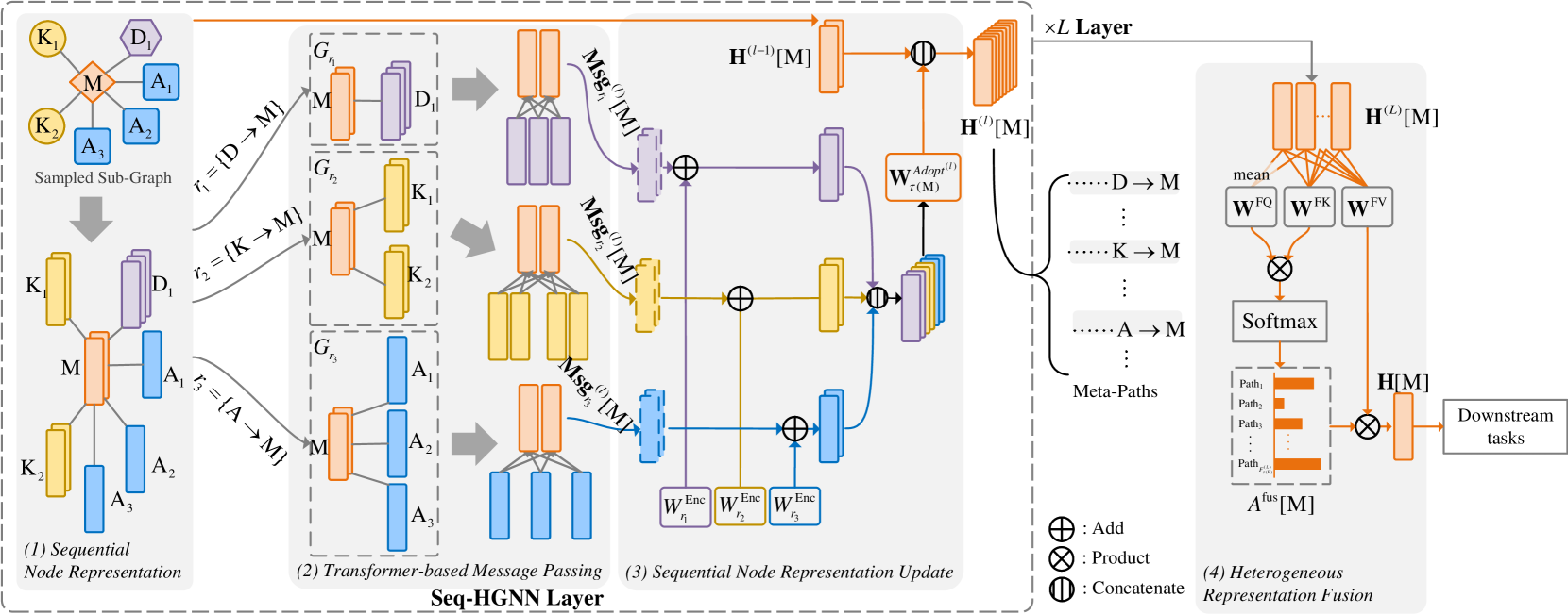
Figure 2. The overview of our proposed Seq-HGNN. Given a heterogeneous sub-graph containing a target node $\mathbf{M}$ and six source nodes, Seq-HGNN  first learns a sequential node representation of $\mathbf{M}$ (i.e. $\mathbf{H}^{(L)}\left[\mathbf{M}\right]$), and then fuses the representation $\mathbf{H}^{(L)}\left[\mathbf{M}\right]$ for multiple downstream tasks. In the sub-graph, $\mathbf{M}$, $\mathbf{K}$, $\mathbf{A}$, and $\mathbf{D}$ represent node types Movie, Keyword, Actor, Director, respectively.

The overview of our proposed Seq-HGNN. Given a heterogeneous sub-graph containing a target node $\mathbf{M}$ and six source nodes, Seq-HGNN  first learns a sequential node representation of $\mathbf{M}$ (i.e. $\mathbf{H}^{(L)}\left[\mathbf{M}\right]$), and then fuses the representation $\mathbf{H}^{(L)}\left[\mathbf{M}\right]$ for multiple downstream tasks. In the sub-graph, $\mathbf{M}$, $\mathbf{K}$, $\mathbf{A}$, and $\mathbf{D}$ represent node types Movie, Keyword, Actor, Director, respectively.

4. Methodology

The overview of the proposed Seq-HGNN  is shown in Figure 2. The Seq-HGNN  is composed of multiple Seq-HGNN  Layers and a Heterogeneous Representation Fusion module. The Seq-HGNN  Layers aggregate the information provided by the source node $s$, and update the representation of the target node $t$. We denote the output representation of the $l$-th layer as $\mathbf{H}^{(l)}$, which is also the input of the ($l+1$)-th layer ($1\leq l\leq L$). By stacking $L$ Seq-HGNN  Layers, each target node $t$ can receive higher-order neighbor information. The Seq-HGNN  Layer consists of three modules: Sequential Node Representation, Transformer-based Message Passing and Sequential Node Representation Update. Among them, the Sequential Node Representation transforms each node into a set of representation vectors. The Transformer-based Message Passing generates neighbor messages for the target node by aggregating the information of neighbors (source nodes). The Sequential Node Representation Update computes a new representation for $t$ based on the representation from the previous layer and the received neighbor messages. Finally, the Heterogeneous Representation Fusion module estimates the importance of meta-paths and fuses the representations of meta-paths to a single vector as node representation, which can be utilized in downstream tasks.

4.1. Sequential Node Representation

In heterogeneous graphs, the nodes often have multiple attributes and receive messages from multiple types of nodes. For example, in a heterogeneous graph from a movie review website, a Movie node usually contains multiple description attributes such as Storyline, Taglines, Release date, etc. Existing methods only support representing each node as a single vector, which implies that the multiple properties of each node are confused into one vector. This causes information loss of node representation.

Different from the above-mentioned graph representation learning methods (Schlichtkrull et al., 2018; Hu et al., 2020a; Yu et al., 2022), we represent each node as one sequence of vectors, which can record multiple properties of node and messages from multiple meta-paths intact. Concretely, given a node $i$, we first design a type-specific transform matrix $W^{\tau(i)}$ to convert features $x^{i}$ of node $i$ to the same space:

(1) $$H^{(0)}_{f}\left[i\right]=W^{\tau(i)}_{f}\cdot x^{i}_{f}+b^{\tau(i)}_{f},$$

where $\tau(i)$ is the node type of node $i$; $1\leq f\leq F^{(0)}_{\tau(i)}$; $F^{(0)}_{\tau(i)}$ is the number of $i$’s features; $x^{i}_{f}$ is the $f$-th initialized feature in the feature sequence of $i$; $H^{(0)}_{f}\left[i\right]\in\mathbb{R}^{d}$ is the node features after the transform; $b^{\tau(i)}_{f}$ is the bias; $d$ is the dimension of features.

Next, we concatenate the $F^{(0)}_{\tau(i)}$ transformed representations of node $i$ to get an input sequence $\mathbf{H}^{(0)}\left[i\right]$ for the Seq-HGNN  model:

(2) $$\mathbf{H}^{(0)}\left[i\right]=\bigg{\Arrowvert}_{f}^{F^{(0)}_{\tau(i)}}H^{(0)}_{f}\left[i\right],$$

where $\bigg{\Arrowvert}$ is the concatenation operation and $\mathbf{H}^{(0)}\left[i\right]\in\mathbb{R}^{F^{(0)}_{\tau(i)}\times d}$ is a sequence with the length of $F^{(0)}_{\tau(i)}$.

It is worth noting that our proposed sequential node representation is independent of time series. During the message passing, our model always represents each node as one sequence of vectors. Each vector in the sequence can represent either the meta-path information or a specific feature attribute of the node. For a detailed description, please refer to Section 4.2 and 4.3.

4.2. Transformer-based Message Passing

The message-passing module aggregates the information of neighbors (source nodes) on each relational bipartite graph to generate neighbor messages for the target node.

4.2.1. Neighbor Importance Estimation

Before the neighbor message generation, we first estimate the importance of these neighbors. We utilize the mutual attention (Vaswani et al., 2017; Hu et al., 2020a) to calculate the importance of source nodes to the target node. Specifically, we first project the representations of the target node $t$ and its neighbors (source nodes $s$) to multiple Query vectors $\mathbf{Q}$ and Key vectors $\mathbf{K}$, respectively.

(3) $$\mathbf{Q}^{(l)}[t]=\bigg{\Arrowvert}_{f}^{F^{(l-1)}_{\tau(t)}}\mathbf{W}^{\text{Query}^{(l)}}_{\tau(t)}H^{(l-1)}_{f}\left[t\right]+b^{\text{Query}^{(l)}}_{\tau(t)},$$

(4) $$\mathbf{K}^{(l)}[s]=\bigg{\Arrowvert}_{f}^{F^{(l-1)}_{\tau(s)}}\mathbf{W}^{\text{Key}^{(l)}}_{\tau(s)}H^{(l-1)}_{f}\left[s\right]+b^{\text{Key}^{(l)}}_{\tau(s)},$$

where $\mathbf{W}^{\text{Query}^{(l)}}_{\tau(t)}\in\mathbb{R}^{d\times d}$ and $\mathbf{W}^{\text{Key}^{(l)}}_{\tau(s)}\in\mathbb{R}^{d\times d}$ are type-specific trainable transformation matrices for source node $s$ and target node $t$; $b^{\text{Query}^{(l)}}_{\tau(t)}$ and $b^{\text{Key}^{(l)}}_{\tau(s)}$ are bias vectors. The shapes of $\mathbf{Q}^{(l)}[t]$ and $\mathbf{K}^{(l)}[s]$ are $F^{(l-1)}_{\tau(t)}\times d$ and $F^{(l-1)}_{\tau(s)}\times d$, respectively. $F^{(l-1)}_{\tau(t)}$ and $F^{(l-1)}_{\tau(s)}$ represent the length of sequence representations of $t$ and $s$ in the ($l-1$) layer, respectively.

We regard the attention weights of the source node $s$ to the target node $t$ as the importance of $s$ to $t$. Since the nodes would play different roles in different relations, we calculate the attention weights on each bipartite graph separately. More specifically, we denote the set of source nodes connected by the target node $t$ in the bipartite graph $G_{r}$ as $N_{r}(t)$, where $r\in\mathbf{R}$. Then, the attention weights can be formulated as:

(5) $$\textbf{Attn}^{(l)}_{r}[s,t]=\underset{\forall s\in N_{r}(t)}{\text{Softmax}}\left(\mathbf{K}^{(l)}[s]W^{\text{ATT}^{(l)}}_{r}{\mathbf{Q}^{(l)}[t]}^{\top}\right)\cdot\frac{1}{\sqrt{d}},$$

where $\textbf{Attn}^{(l)}_{r}[s,t]$ is the importance estimation of the source node $s$ to the target node $t$ on relation $r$, and $W^{\text{ATT}^{(l)}}_{r}\in\mathbb{R}^{d\times d}$ is the transform matrix for relation $r$.

Unlike the existing attention-based approaches (Yu et al., 2022; Hu et al., 2020a; Velickovic et al., 2018), the attention weight $\textbf{Attn}^{(l)}_{r}[s,t]$ is a matrix with the shape $F^{(l-1)}_{\tau(s)}\times F^{(l-1)}_{\tau(t)}$ rather than a scalar. Each element in $\textbf{Attn}^{(l)}_{r}[s,t]$ represents the attention weight of an item in the representation sequence of $s$ to an item in the representation sequence of $t$.

4.2.2. Neighbor Message Generation

According to the importance of neighbors, the Seq-HGNN  aggregates the neighbor information and treats it as the neighbor messages for $t$.

First, Seq-HGNN  extracts features of the source node $s$ in each bipartite graph $G_{r}$ separately as follows:

(6) $$\textbf{Ext}^{(l)}_{r}[s]=\bigg{\Arrowvert}_{f}^{F^{(l-1)}_{\tau(s)}}W^{\text{EXT}^{(l)}}_{r}\left(\mathbf{W}^{\text{Value}^{(l)}}_{\tau(s)}H^{(l-1)}_{f}\left[s\right]+b^{\text{Value}^{(l)}}_{\tau(s)}\right),$$

where $\textbf{Ext}^{(l)}_{r}[s]\in\mathbb{R}^{F^{(l-1)}_{\tau(s)}\times d}$ is the extracted message from the source node $s$ under the relation $r$; $\mathbf{W}^{\text{Value}^{(l)}}_{\tau(s)}\in\mathbb{R}^{d\times d}$ is the transformation matrix for for the node type $\tau(s)$; $b^{\text{Value}^{(l)}}$ is the bias; $W^{\text{EXT}^{(l)}}_{r}$ is the transform matrix for the relation $r$.

Then, we can obtain the neighbor messages for $t$ under relation $r$ as follows:

(7) $$\textbf{Msg}^{(l)}_{r}[t]=\underset{\forall s\in N_{r}(t)}{\sum}\left({\textbf{Attn}^{(l)}_{r}[s,t]}^{\top}\textbf{Ext}^{(l)}_{r}[s]\right),$$

where $\textbf{Msg}^{(l)}_{r}[t]\in\mathbb{R}^{F^{(l-1)}_{\tau(t)}\times d}$ is a sequence with the same shape as the node representation $\mathbf{H}^{(l-1)}\left[t\right]$, and $N_{r}(t)$ is the set of neighbors (source nodes) of the target node $t$ in the bipartite graph $G_{r}$.

4.3. Sequential Node Representation Update

After the message passing process, the target node $t$ receives messages $\textbf{Msg}^{(l)}_{r}[t]$ from multiple relations $r\in R$. Based on the received messages and the representations from the previous layer $\mathbf{H}^{(l-1)}\left[t\right]$, we get the updated node representation of $t$.

First, we concatenate the message sequences from different relation types with relation-aware encoding as follows:

(8) $$\widetilde{\mathbf{H}}^{(l)}\left[t\right] =\underset{\forall r\in R(t)}{\Arrowvert}\widetilde{\textbf{Msg}}^{(l)}_{r}[t],$$

(9) $$\widetilde{\textbf{Msg}}^{(l)}_{r}[t] =\textbf{Msg}^{(l)}_{r}[t]\oplus W_{r}^{\text{Enc}},$$

where $R(t)$ is the set of relation types whose target node type is $\tau(t)$; $W_{r}^{\text{Enc}}\in\mathbb{R}^{d}$ is the relation encoding for relation $r$, which is a learnable vector to distinguish messages from different relation types; $\oplus$ represents that the relation encoding is added to each vector in the sequence.

Then, we concatenate the representations of the target node from the last layer and encoded messages to obtain a new representation of the target node $t$:

(10) $$\mathbf{H}^{(l)}\left[t\right]=\mathbf{H}^{(l-1)}\left[t\right]\quad\Arrowvert\quad\mathbf{W}^{\text{Adopt}^{(l)}}_{\tau(t)}\widetilde{\mathbf{H}}^{(l)}\left[t\right],$$

where $\mathbf{H}^{(l)}\left[t\right]\in\mathbb{R}^{F^{(l)}_{\tau(t)}\times d}$ is the updated representations of target node $t$; $\mathbf{W}^{\text{Adopt}^{(l)}}_{\tau(t)}\in\mathbb{R}^{d\times d}$ is a transformation matrix corresponding to the $\tau(t)$.

We denote that the number of relation types connected to the target node $t$ is $\text{len}(R(t))$, then the length of the sequential representations for target node $t$ grows according to the following:

(11) $$F^{(l)}_{\tau(t)}=F^{(l-1)}_{\tau(t)}\times\left(\text{len}(R(t))+1\right),$$

where $F^{(l-1)}_{\tau(t)}$ and $F^{(l)}_{\tau(t)}$ represent the length of the sequential representation for node $t$ in the $(l-1)$-th and $l$-th layers, respectively. Referring to Equation 10 and Equation 11, we can summarize that in sequential node representation, information from a node itself and low-order neighbors is located at the beginning of the sequence, followed by high-order information. As deeper Seq-HGNN Layers are performed, information from higher-order neighbors is appended to the sequence.

4.4. Heterogeneous Representation Fusion

After the $L$-layer Seq-HGNN  computation, each target node $t$ is represented by a sequence with length $F^{(L)}_{\tau(t)}$, which are the representations of the $t$ from multiple meta-paths. We utilize the self attention (Vaswani et al., 2017) mechanism to fuse the sequential representations of the target node $t$ into a single vector. During the representation fusion, Seq-HGNN  can identify the effective meta-paths for downstream tasks.

$$Q^{\text{fus}}[t] =\text{mean}\left(\mathbf{H}^{(0)}\left[t\right]W^{\text{FQ}}\right),$$

$$K^{\text{fus}}[t] =\mathbf{H}^{(L)}\left[t\right]W^{\text{FK}},$$

$$V^{\text{fus}}[t] =\mathbf{H}^{(L)}\left[t\right]W^{\text{FV}},$$

$$A^{\text{fus}}[t] =\text{Softmax}\left(\frac{Q^{\text{fus}}[t]{K^{\text{fus}}[t]}^{\top}}{\sqrt{d}}\right),$$

(12) $$\mathbf{H}\left[t\right] =A^{\text{fus}}[t]V^{\text{fus}}[t],$$

where $\mathbf{H}\left[t\right]\in\mathbb{R}^{d}$ is the final representation of the target node $t$; $W^{\text{FQ}}$, $W^{\text{FK}}$ and $W^{\text{FV}}$ are all learnable matrices of dimension $d\times d$; $Q^{\text{fus}}[t]$ is generated by original features of target node $t$; $A^{\text{fus}}[t]\in\mathbb{R}^{F^{(l)}_{\tau(i)}}$ stands for the importance of each representation for node $t$, which is also the importance of meta-paths.

Referring to (Velickovic et al., 2018; Hu et al., 2020a; Yu et al., 2022), we adopt the multi-head attention mechanism during the message passing and representation fusion. The output of the multi-head attention is concatenated into a $d$-dimensional representation to enhance the stability of the model. In addition, we randomly drop out some fragments of the sequential representation of each node in training loops, which can help the Seq-HGNN  model learn more meaningful node representations.

5. Experiments

In this section, we evaluate the performance of Seq-HGNN  by conducting experiments on multiple datasets.

5.1. Datasets

We conduct extensive experiments on four widely used datasets from Heterogeneous Graph Benchmark (HGB) (Lv et al., 2021) and Open Graph Benchmark (OGB) (Hu et al., 2020b). Specifically, three medium-scale datasets, DBLP, IMDB and ACM, are from HGB. A large-scale dataset MAG comes from OGB. Their statistics are shown in Table 1.

• DBLP is a bibliography website of computer science. This dataset contains four types of nodes: Author, Paper, Term and Venue. In this data set, models need to predict the research fields of authors.

• IMDB is extracted from the Internet Movie Database (IMDb). It contains four types of nodes: Movie, Director, Keyword and Actor. Models need to divide the movie into 5 categories: “Romance”, “Thriller”, “Comedy”, “Action, Drama”.

• ACM is also a citation network. It contains four types of nodes: Paper, Author, Subject (Conference) and Term. The Paper nodes are divided into 3 categories: ”database“, ”wireless communication“ and “data mining”. The model needs to predict the category the paper belongs to.

• MAG is a heterogeneous academic network extracted from the Microsoft Academic Graph, consisting of Paper, Author, Field and Institution. Papers are published in 349 different venues. Each paper is associated with a Word2Vec feature. The model needs to predict the category the paper belongs to. The model needs to predict the venues in which the papers are published.

Table 1. Statistics of datasets.

name	#Nodes	#Node Types	#Edges	#Edge Types	Target	#Classes
DBLP	26,128	4	239,566	6	author	4
IMDB	21,420	4	86,642	6	movie	5
ACM	10,942	4	547,872	8	paper	3
MAG	1,939,743	4	21,111,007	4	paper	349

		DBLP		IMDB		ACM
		macro-f1	micro-f1	macro-f1	micro-f1	macro-f1	micro-f1
Metapath-based methods	RGCN	91.52±0.50	92.07±0.50	58.85±0.26	62.05±0.15	91.55±0.74	91.41±0.75
	HetGNN	91.76±0.43	92.33±0.41	48.25±0.67	51.16±0.65	85.91±0.25	86.05±0.25
	HAN	91.67±0.49	92.05±0.62	57.74±0.96	64.63±0.58	90.89±0.43	90.79±0.43
	MAGNN	93.28±0.51	93.76±0.45	56.49±3.20	64.67±1.67	90.88±0.64	90.77±0.65
Metapath-free methods	RSHN	93.34±0.58	93.81±0.55	59.85±3.21	64.22±1.03	90.50±1.51	90.32±1.54
	HetSANN	78.55±2.42	80.56±1.50	49.47±1.21	57.68±0.44	90.02±0.35	89.91±0.37
	HGT	93.01±0.23	93.49±0.25	63.00±1.19	67.20±0.57	91.12±0.76	91.00±0.76
	HGB	94.01±0.24	94.46±0.22	63.53±1.36	67.36±0.57	93.42±0.44	93.35±0.45
	SeHGNN	95.06±0.17	95.42±0.17	67.11±0.25	69.17±0.43	94.05±0.35	93.98±0.36
Ours	Seq-HGNN	96.27±0.24	95.96±0.31	66.77±0.24	69.31±0.27	94.41±0.26	94.33±0.31
	-w/o seq	93.79±0.34	93.51±0.38	64.32±0.56	67.04±0.62	92.44±0.67	92.17±0.72
	-w/o fus	95.59±0.14	95.92±0.13	65.01±0.37	67.43±0.32	93.21±0.48	93.20±0.50
	-w/o rel	95.49±0.23	95.64±0.18	64.78±0.41	69.09±0.39	93.76 ±0.43	93.67±0.46

Table 2. Experiment results on the three datasets from the HGB benchmark. The best results are in bold, and the second-best results are underlined.

Methods	Validation accuracy	Test accuracy
RGCN	48.35±0.36	47.37±0.48
HGT	49.89±0.47	49.27±0.61
NARS	51.85±0.08	50.88±0.12
SAGN	52.25±0.30	51.17±0.32
GAMLP	53.23±0.23	51.63±0.22
HGT+emb	51.24±0.46	49.82±0.13
NARS+emb	53.72±0.09	52.40±0.16
GAMLP+emb	55.48±0.08	53.96±0.18
SAGN+emb+ms	55.91±0.17	54.40±0.15
GAMLP+emb+ms	57.02±0.41	55.90±0.27
SeHGNN+emb	56.56±0.07	54.78±0.17
SeHGNN+emb+ms	59.17±0.09	57.19±0.12
Seq-HGNN+emb	56.93±0.11	55.27±0.34
Seq-HGNN+emb+ms	59.21±0.08	57.76±0.26

Table 3. Experiment results on the large-scale dataset MAG, where “emb” means using extra embeddings and “ms” means using multi-stage training. The best results are in bold, and the second-best results are underlined.

5.2. Results Analysis

5.2.1. Results on HGB Benchmark

Table 3 shows the results of Seq-HGNN  on the three datasets compared to the baselines in the HGB benchmark. Baselines are divided into two categories: meta-path-based methods and meta-path-free methods. Meta-path based methods include RGCN (Schlichtkrull et al., 2018), HetGNN (Zhang et al., 2019), HAN (Wang et al., 2019) and MAGNN (Fu et al., 2020). The meta-path-free methods are RSHN (Zhu et al., 2019), HetSANN (Hong et al., 2020b), HGT (Hu et al., 2020a), HGB (Lv et al., 2021) and SeHGNN (Yang et al., 2022). The results of the baselines are from HGB and their original papers. As shown in Table 3, our proposed method achieves the best performance on ACM and DBLP datasets. In detail, Seq-HGNN  gains improvement beyond the best baseline on macro-f1 by (1.2%, 0.4%) and on mirco-f1 by (0.5%, 0.4%), respectively. On the IMDB dataset, our method achieves the best micro f1 scores and the second-best macro f1 scores. The performance difference between IMDB and the other two datasets may be due to the following two reasons: (1) Domain difference: DBLP and ACM are datasets in the academic domain while IMDB comes from the film domain. (2) Task difference: IMDB is a multiple-label classification task, but ACM and DBLP are not.

5.2.2. Results on OGB-MAG

Since some types of nodes in the MAG dataset have no initial features, existing methods usually utilize unsupervised representation methods to generate node embeddings (abbreviated as emb) as initial features. For a fair comparison, we also use the unsupervised representation learning method (ComplEx (Trouillon et al., 2016)) to generate node embeddings. In addition, some baseline methods on the list also adopt multi-stage learning (Li et al., 2018; Sun et al., 2020; Yang et al., 2021b) (abbreviated as ms) tricks to improve the generalization ability of the model. Therefore, we also explored the performance of Seq-HGNN  under the multi-stage training.

As shown in Table 3, Seq-HGNN  achieves the best performance compared to the baseline on the ogb leaderboard . It shows that our method can not only mine information in heterogeneous graphs more effectively, but also reflect good scalability to be applied to large-scale graphs.

5.3. Ablation Study

One of the core contributing components in Seq-HGNN is to explore how to effectively exploit the structural information in heterogeneous graphs. So we design three variants of our model to verify their effects, namely Seq-HGNN  w/o seq, Seq-HGNN  w/o fus, and Seq-HGNN  w/o rel. The performance of these variants on the HGB dataset is shown in Table 2. The details of these variants are as follows:

• Seq-HGNN  w/o seq. It does not use the sequential node representation. After each layer of graph convolution, multiple node representations from different relationships are aggregated into a vector representation by the mean operation. Finally, the Seq-HGNN  w/o seq concatenates the output of each graph convolutional layer as the final output for the downstream tasks. Comparing Seq-HGNN  w/o seq and Seq-HGNN, it can be found that after introducing sequential node representation, the performance of the model can be significantly improved. It proves that sequential node representations indeed retain richer and more effective node information.

• Seq-HGNN  w/o fus. It works on the final representation of the node, in which it drops the heterogeneous representation fusion module, instead using the average representation sequence output sent by the last layer of Seq-HGNN. Comparing Seq-HGNN  w/o fus and Seq-HGNN, it can be found that the performance decreases after removing the heterogeneous fusion module. It illustrates the importance of recognizing the most contributing meta-path.

• Seq-HGNN  w/o rel. It does not add relationship-aware encoding when updating the node representation, which is introduced in equation 9, section 4.3. As shown in Table 3, Seq-HGNN  performs better than Seq-HGNN  w/o rel on all datasets. It verifies the relation-distinguishing ability of Seq-HGNN.

5.4. Experiment Setup Detail

We use the PyTorch Geometric framework 2.0 to implement the Seq-HGNN. The source code is available at https://github.com/nobrowning/SEQ_HGNN. We set the node embedding dimension $d=512$, and the number of attention heads to 8. The number of layers $L$ is set to 2 on the DBLP, IMDB and MAG datasets and to 3 on the ACM dataset. During the training process, we set the dropout rate to 0.5, and the maximum epoch to 150. We use the AdamW optimizer (Loshchilov and Hutter, 2019) with a maximum learning rate of 0.0005 and tune the learning rate using the OneCycleLR strategy (Smith and Topin, 2019). For DBLP, ACM, and IMDB datasets, we use full batch training. For the large-scale dataset MAG, we use the HGTLoader subgraph sampling strategy (Hu et al., 2020a), setting the batch size to 256, sampling depth to 3, sample number to 1800. We iterate 250 batches in each epoch.

The results of the baselines in Table 2 and Table 3 mainly come from previous works (Lv et al., 2021; Yang et al., 2022). All experiments can be conducted on a Linux machine with Intel(R) Core(R) i7 8700 CPU, 32G RAM, and a single NVIDIA GeForce RTX 3090 GPU.

5.5. Training Efficiency

In Seq-HGNN, sequential node representations are computed in parallel. Therefore, Seq-HGNN  achieves decent computational efficiency. To further investigate the computational efficiency of Seq-HGNN, we conduct experiments to compare the training time of Seq-HGNN  with a state-of-the-art baseline, i.e., SeHGNN.

To achieve a fair comparison, we subject all models to the same accuracy performance validation — making a test on the test set every one train epoch. The variation of test accuracy of the models with training time is shown in Figure 3.

As shown in Figure 3, Seq-HGNN  performs the highest accuracy within the least training time. It verifies that Seq-HGNN  has good computational efficiency when dealing with heterogeneous graphs. As a comparison, the baseline (SeHGNN) outputs nothing within 42 seconds of starting training. The reason is that SeHGNN cannot directly learn node representations on heterogeneous graphs. It requires a message-passing step before node representation generation. In the message passing step, SeHGNN collects the features of neighbor nodes of the target on all meta-paths. Therefore, the messaging step shows a high time-consuming.

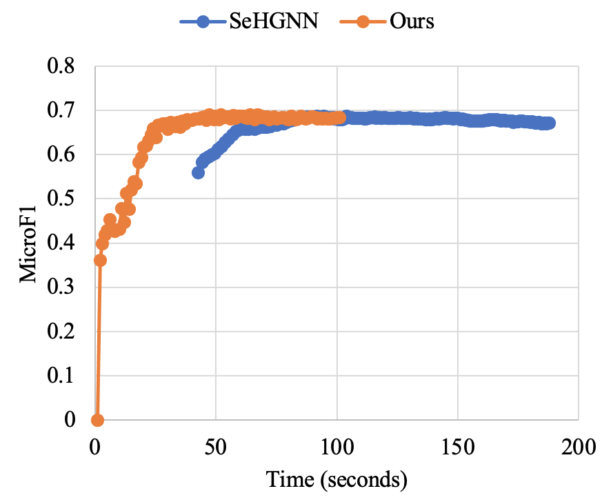
Figure 3. The comparison of training efficiency.

The comparison of training efficiency.

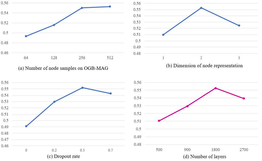
Figure 4. Parameter Sensitivity of Seq-HGNN.

Parameter Sensitivity of Seq-HGNN.

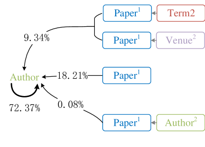
(a) DBLP.

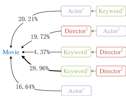
(b) IMDB.

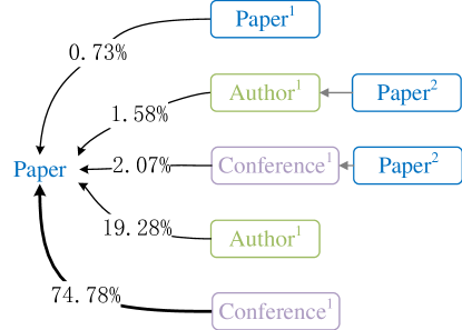
(c) ACM.

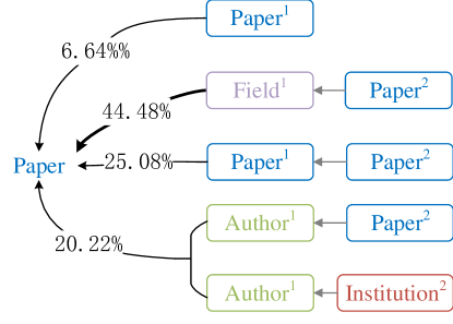
(d) MAG.

Figure 5. Visualization of the significant meta-paths for representing the target nodes (Author, Movie, Paper, Paper) in respective datasets (DBLP, IMDB, ACM, MAG). In the figures, the nodes with superscripts $1$ and $2$ represent the direct neighbors and the second-order neighbors of the target node, respectively.

Visualization of the significant meta-paths for representing the target nodes (Author, Movie, Paper, Paper) in respective datasets (DBLP, IMDB, ACM, MAG). In the figures, the nodes with superscripts $1$ and $2$ represent the direct neighbors and the second-order neighbors of the target node, respectively.

5.6. Parameter Sensitivity Analysis

We study the sensitivity analysis of parameters in Seq-HGNN. Specifically, we conduct experiments on the large-scale dataset OGB-MAG to explore the influence of the number of layers, the dropout rate, and the dimension of node representation. Since the model needs to conduct a sub-graph sampling on the large-scale dataset, we also explore the influence of sampling node numbers. To simplify the evaluation process, we opted not to employ a multi-stage training strategy in the parameter sensitivity experiment. The results are shown in Figure 4, where each subfigure shows the accuracy of classification on the y-axis and hyperparameters on the x-axis.

5.6.1. Number of node samples.

Since Seq-HGNN  uses HGT-Loader for sampling sub-graphs in the node classification task, we explore the effect of node sampling number on the performance of Seq-HGNN. As shown in Figure 4 (a), Seq-HGNN  achieves the best performance when the number of samples is set as 1800.

5.6.2. Dimension of node representation.

We report the experimental result varied with the dimension of node representation in Figure 4 (b). It can be seen that as the dimension increases, the performance of Seq-HGNN  gradually increases. After the dimension is higher than 256, the performance improvement slows down.

5.6.3. Dropout rate.

We adjust the dropout rate during the model training and report the results in Figure 4 (c). We can observe that Seq-HGNN  performs best when the dropout rate is 0.5. A high dropout rate would lead to underfitting and poor performance, while a low dropout rate may lead to overfitting.

5.6.4. Number of layers.

We explore the performance of our model while stacking from 1 to 3 Seq-HGNN  Layers. The experimental results are shown in Figure 4 (d). It can be seen that Seq-HGNN  achieves the best performance when it is stacked with 2 layers. On this basis, the performance of Seq-HGNN  becomes worse when more layers are stacked. This may be caused by over-smoothing issues.

5.7. Visualization of Effective Meta-Paths

As mentioned in Section 4.4, $A^{\text{fus}}$ in the Heterogeneous Representation Fusion module indicates the importance of different representations of a node, i.e., the importance of a node on different meta-paths. To visualize how the heterogeneous fusion module of Seq-HGNN  identifies the most contributing meta-paths, we present the effective meta-paths in node representation learning on DBLP, IMDB, ACM and MAG datasets, respectively. The most important meta-paths for these target node representations are shown in Figure 5. It is noteworthy that our model can individually identify the significant metapaths characterizing each node. In order to simplify the visualization, we aggregate the propagation path weights of nodes by node type in Figure 5. Due to the large number of meta-paths, here, we only show the top five important paths in each sub-figure.

Comparing the four sub-figure in Figure 5, we can find that the important paths for distinct nodes are obviously different. It verifies that the Seq-HGNN  can estimate the path importance separately for different nodes, rather than treat them equally.

In sub-figure (a), we can observe that the self-loop of the target node (Author) has a high weight (72.37%). It reveals that in the ACM dataset, the representation of the Author node mainly depends on its own attributes rather than the structural information in the graph. In contrast, the information of the target node (Movie) in sub-figure (b) mainly comes from its neighbor nodes. The target node types in sub-figure (c) and sub-figure (d) are both Paper. However, there is a significant difference between sub-figure (c) and sub-figure (d): the most important meta-path in sub-figure (c) is “Paper-Conference”, while the information of the target node in sub-figure (d) mostly comes from the meta-paths related to Paper, such as “Paper-Field-Paper”, “Paper-Paper-Paper”, “Paper-Author-Paper”, etc. The difference between sub-figure (c) and sub-figure (d) may be mainly caused by their downstream tasks. Specifically, the task of sub-figure (c) is to predict the field of the paper while the task of sub-figure (d) is to predict the journal where the paper is published. This indicates that our model can utilize different aspects of graphs according to different downstream task demands. By mining important propagation paths, the model can provide deep insights and interpretability into the real-world application scenarios.

6. Conclusion

In this paper, we proposed a novel heterogeneous graph neural network with sequential node representation, namely Seq-HGNN. To avoid the information loss caused by the single vector node representation, we first design a sequential node representation learning mechanism to represent each node as a sequence of meta-path representations during the node message passing. Then we propose a heterogeneous representation fusion module, empowering Seq-HGNN  to identify important meta-paths and aggregate their representations into a compact one. Third, we conducted extensive experiments on four widely-used datasets from open benchmarks and clearly validated the effectiveness of our model. Finally, we visualized and analyzed effective meta-path paths in different datasets, and verified that Seq-HGNN  can provide deep insights into the heterogeneous graphs.

- (1)
- Cai et al. (2022) Desheng Cai, Shengsheng Qian, Quan Fang, Jun Hu, and Changsheng Xu. 2022. User Cold-Start Recommendation via Inductive Heterogeneous Graph Neural Network. ACM Trans. Inf. Syst. (sep 2022). https://doi.org/10.1145/3560487 Just Accepted.
- Chen et al. (2022) Dapeng Chen, Min Wang, Haobin Chen, Lin Wu, Jing Qin, and Wei Peng. 2022. Cross-Modal Retrieval with Heterogeneous Graph Embedding. In MM ’22: The 30th ACM International Conference on Multimedia, Lisboa, Portugal, October 10 - 14, 2022, João Magalhães, Alberto Del Bimbo, Shin’ichi Satoh, Nicu Sebe, Xavier Alameda-Pineda, Qin Jin, Vincent Oria, and Laura Toni (Eds.). ACM, 3291–3300. https://doi.org/10.1145/3503161.3548195
- Feng et al. (2022) Yue Feng, Zhen Han, Mingming Sun, and Ping Li. 2022. Multi-Hop Open-Domain Question Answering over Structured and Unstructured Knowledge. In Findings of the Association for Computational Linguistics: NAACL 2022, Seattle, WA, United States, July 10-15, 2022, Marine Carpuat, Marie-Catherine de Marneffe, and Iván Vladimir Meza Ruíz (Eds.). Association for Computational Linguistics, 151–156. https://doi.org/10.18653/v1/2022.findings-naacl.12
- Fu et al. (2020) Xinyu Fu, Jiani Zhang, Ziqiao Meng, and Irwin King. 2020. MAGNN: Metapath Aggregated Graph Neural Network for Heterogeneous Graph Embedding. In WWW ’20: The Web Conference 2020, Taipei, Taiwan, April 20-24, 2020, Yennun Huang, Irwin King, Tie-Yan Liu, and Maarten van Steen (Eds.). ACM / IW3C2, 2331–2341. https://doi.org/10.1145/3366423.3380297
- Gao et al. (2022) Shen Gao, Yuchi Zhang, Yongliang Wang, Yang Dong, Xiuying Chen, Dongyan Zhao, and Rui Yan. 2022. HeteroQA: Learning towards Question-and-Answering through Multiple Information Sources via Heterogeneous Graph Modeling. In WSDM ’22: The Fifteenth ACM International Conference on Web Search and Data Mining, Virtual Event / Tempe, AZ, USA, February 21 - 25, 2022, K. Selcuk Candan, Huan Liu, Leman Akoglu, Xin Luna Dong, and Jiliang Tang (Eds.). ACM, 307–315. https://doi.org/10.1145/3488560.3498378
- Guan et al. (2022) Weili Guan, Fangkai Jiao, Xuemeng Song, Haokun Wen, Chung-Hsing Yeh, and Xiaojun Chang. 2022. Personalized Fashion Compatibility Modeling via Metapath-guided Heterogeneous Graph Learning. In SIGIR ’22: The 45th International ACM SIGIR Conference on Research and Development in Information Retrieval, Madrid, Spain, July 11 - 15, 2022, Enrique Amigó, Pablo Castells, Julio Gonzalo, Ben Carterette, J. Shane Culpepper, and Gabriella Kazai (Eds.). ACM, 482–491. https://doi.org/10.1145/3477495.3532038
- Hong et al. (2020a) Huiting Hong, Hantao Guo, Yucheng Lin, Xiaoqing Yang, Zang Li, and Jieping Ye. 2020a. An Attention-Based Graph Neural Network for Heterogeneous Structural Learning. In The Thirty-Fourth AAAI Conference on Artificial Intelligence, AAAI 2020, The Thirty-Second Innovative Applications of Artificial Intelligence Conference, IAAI 2020, The Tenth AAAI Symposium on Educational Advances in Artificial Intelligence, EAAI 2020, New York, NY, USA, February 7-12, 2020. AAAI Press, 4132–4139. https://ojs.aaai.org/index.php/AAAI/article/view/5833
- Hong et al. (2020b) Huiting Hong, Hantao Guo, Yucheng Lin, Xiaoqing Yang, Zang Li, and Jieping Ye. 2020b. An Attention-Based Graph Neural Network for Heterogeneous Structural Learning. In The Thirty-Fourth AAAI Conference on Artificial Intelligence, AAAI 2020, The Thirty-Second Innovative Applications of Artificial Intelligence Conference, IAAI 2020, The Tenth AAAI Symposium on Educational Advances in Artificial Intelligence, EAAI 2020, New York, NY, USA, February 7-12, 2020. AAAI Press, 4132–4139. https://ojs.aaai.org/index.php/AAAI/article/view/5833
- Hu et al. (2020b) Weihua Hu, Matthias Fey, Marinka Zitnik, Yuxiao Dong, Hongyu Ren, Bowen Liu, Michele Catasta, and Jure Leskovec. 2020b. Open Graph Benchmark: Datasets for Machine Learning on Graphs. In Advances in Neural Information Processing Systems 33: Annual Conference on Neural Information Processing Systems 2020, NeurIPS 2020, December 6-12, 2020, virtual, Hugo Larochelle, Marc’Aurelio Ranzato, Raia Hadsell, Maria-Florina Balcan, and Hsuan-Tien Lin (Eds.). https://proceedings.neurips.cc/paper/2020/hash/fb60d411a5c5b72b2e7d3527cfc84fd0-Abstract.html
- Hu et al. (2020a) Ziniu Hu, Yuxiao Dong, Kuansan Wang, and Yizhou Sun. 2020a. Heterogeneous Graph Transformer. In WWW ’20: The Web Conference 2020, Taipei, Taiwan, April 20-24, 2020, Yennun Huang, Irwin King, Tie-Yan Liu, and Maarten van Steen (Eds.). ACM / IW3C2, 2704–2710. https://doi.org/10.1145/3366423.3380027
- Li et al. (2018) Qimai Li, Zhichao Han, and Xiao-Ming Wu. 2018. Deeper Insights Into Graph Convolutional Networks for Semi-Supervised Learning. In Proceedings of the Thirty-Second AAAI Conference on Artificial Intelligence, (AAAI-18), the 30th innovative Applications of Artificial Intelligence (IAAI-18), and the 8th AAAI Symposium on Educational Advances in Artificial Intelligence (EAAI-18), New Orleans, Louisiana, USA, February 2-7, 2018, Sheila A. McIlraith and Kilian Q. Weinberger (Eds.). AAAI Press, 3538–3545. https://www.aaai.org/ocs/index.php/AAAI/AAAI18/paper/view/16098
- Loshchilov and Hutter (2019) Ilya Loshchilov and Frank Hutter. 2019. Decoupled Weight Decay Regularization. In 7th International Conference on Learning Representations, ICLR 2019, New Orleans, LA, USA, May 6-9, 2019. OpenReview.net. https://openreview.net/forum?id=Bkg6RiCqY7
- Lv et al. (2021) Qingsong Lv, Ming Ding, Qiang Liu, Yuxiang Chen, Wenzheng Feng, Siming He, Chang Zhou, Jianguo Jiang, Yuxiao Dong, and Jie Tang. 2021. Are we really making much progress?: Revisiting, benchmarking and refining heterogeneous graph neural networks. In KDD ’21: The 27th ACM SIGKDD Conference on Knowledge Discovery and Data Mining, Virtual Event, Singapore, August 14-18, 2021, Feida Zhu, Beng Chin Ooi, and Chunyan Miao (Eds.). ACM, 1150–1160. https://doi.org/10.1145/3447548.3467350
- Pang et al. (2022) Yitong Pang, Lingfei Wu, Qi Shen, Yiming Zhang, Zhihua Wei, Fangli Xu, Ethan Chang, Bo Long, and Jian Pei. 2022. Heterogeneous Global Graph Neural Networks for Personalized Session-based Recommendation. In WSDM ’22: The Fifteenth ACM International Conference on Web Search and Data Mining, Virtual Event / Tempe, AZ, USA, February 21 - 25, 2022, K. Selcuk Candan, Huan Liu, Leman Akoglu, Xin Luna Dong, and Jiliang Tang (Eds.). ACM, 775–783. https://doi.org/10.1145/3488560.3498505
- Schlichtkrull et al. (2018) Michael Sejr Schlichtkrull, Thomas N. Kipf, Peter Bloem, Rianne van den Berg, Ivan Titov, and Max Welling. 2018. Modeling Relational Data with Graph Convolutional Networks. In The Semantic Web - 15th International Conference, ESWC 2018, Heraklion, Crete, Greece, June 3-7, 2018, Proceedings (Lecture Notes in Computer Science, Vol. 10843), Aldo Gangemi, Roberto Navigli, Maria-Esther Vidal, Pascal Hitzler, Raphaël Troncy, Laura Hollink, Anna Tordai, and Mehwish Alam (Eds.). Springer, 593–607. https://doi.org/10.1007/978-3-319-93417-4_38
- Smith and Topin (2019) Leslie N Smith and Nicholay Topin. 2019. Super-convergence: Very fast training of neural networks using large learning rates. In Artificial intelligence and machine learning for multi-domain operations applications, Vol. 11006. SPIE, 369–386.
- Song et al. (2022) Yaguang Song, Xiaoshan Yang, and Changsheng Xu. 2022. Self-Supervised Calorie-Aware Heterogeneous Graph Networks for Food Recommendation. ACM Trans. Multimedia Comput. Commun. Appl. (mar 2022). https://doi.org/10.1145/3524618 Just Accepted.
- Sun et al. (2020) Ke Sun, Zhouchen Lin, and Zhanxing Zhu. 2020. Multi-Stage Self-Supervised Learning for Graph Convolutional Networks on Graphs with Few Labeled Nodes. In The Thirty-Fourth AAAI Conference on Artificial Intelligence, AAAI 2020, The Thirty-Second Innovative Applications of Artificial Intelligence Conference, IAAI 2020, The Tenth AAAI Symposium on Educational Advances in Artificial Intelligence, EAAI 2020, New York, NY, USA, February 7-12, 2020. AAAI Press, 5892–5899. https://ojs.aaai.org/index.php/AAAI/article/view/6048
- Trouillon et al. (2016) Théo Trouillon, Johannes Welbl, Sebastian Riedel, Éric Gaussier, and Guillaume Bouchard. 2016. Complex Embeddings for Simple Link Prediction. In Proceedings of the 33nd International Conference on Machine Learning, ICML 2016, New York City, NY, USA, June 19-24, 2016 (JMLR Workshop and Conference Proceedings, Vol. 48), Maria-Florina Balcan and Kilian Q. Weinberger (Eds.). JMLR.org, 2071–2080. http://proceedings.mlr.press/v48/trouillon16.html
- Vaswani et al. (2017) Ashish Vaswani, Noam Shazeer, Niki Parmar, Jakob Uszkoreit, Llion Jones, Aidan N. Gomez, Lukasz Kaiser, and Illia Polosukhin. 2017. Attention is All you Need. In Advances in Neural Information Processing Systems 30: Annual Conference on Neural Information Processing Systems 2017, December 4-9, 2017, Long Beach, CA, USA, Isabelle Guyon, Ulrike von Luxburg, Samy Bengio, Hanna M. Wallach, Rob Fergus, S. V. N. Vishwanathan, and Roman Garnett (Eds.). 5998–6008. https://proceedings.neurips.cc/paper/2017/hash/3f5ee243547dee91fbd053c1c4a845aa-Abstract.html
- Velickovic et al. (2018) Petar Velickovic, Guillem Cucurull, Arantxa Casanova, Adriana Romero, Pietro Liò, and Yoshua Bengio. 2018. Graph Attention Networks. In 6th International Conference on Learning Representations, ICLR 2018, Vancouver, BC, Canada, April 30 - May 3, 2018, Conference Track Proceedings. OpenReview.net. https://openreview.net/forum?id=rJXMpikCZ
- Wang et al. (2019) Xiao Wang, Houye Ji, Chuan Shi, Bai Wang, Yanfang Ye, Peng Cui, and Philip S. Yu. 2019. Heterogeneous Graph Attention Network. In The World Wide Web Conference, WWW 2019, San Francisco, CA, USA, May 13-17, 2019, Ling Liu, Ryen W. White, Amin Mantrach, Fabrizio Silvestri, Julian J. McAuley, Ricardo Baeza-Yates, and Leila Zia (Eds.). ACM, 2022–2032. https://doi.org/10.1145/3308558.3313562
- Wang et al. (2021) Xiao Wang, Nian Liu, Hui Han, and Chuan Shi. 2021. Self-supervised Heterogeneous Graph Neural Network with Co-contrastive Learning. In KDD ’21: The 27th ACM SIGKDD Conference on Knowledge Discovery and Data Mining, Virtual Event, Singapore, August 14-18, 2021, Feida Zhu, Beng Chin Ooi, and Chunyan Miao (Eds.). ACM, 1726–1736. https://doi.org/10.1145/3447548.3467415
- Wu et al. (2019) Felix Wu, Amauri H. Souza Jr., Tianyi Zhang, Christopher Fifty, Tao Yu, and Kilian Q. Weinberger. 2019. Simplifying Graph Convolutional Networks. In Proceedings of the 36th International Conference on Machine Learning, ICML 2019, 9-15 June 2019, Long Beach, California, USA (Proceedings of Machine Learning Research, Vol. 97), Kamalika Chaudhuri and Ruslan Salakhutdinov (Eds.). PMLR, 6861–6871. http://proceedings.mlr.press/v97/wu19e.html
- Yang et al. (2021b) Han Yang, Xiao Yan, Xinyan Dai, Yongqiang Chen, and James Cheng. 2021b. Self-Enhanced GNN: Improving Graph Neural Networks Using Model Outputs. In International Joint Conference on Neural Networks, IJCNN 2021, Shenzhen, China, July 18-22, 2021. IEEE, 1–8. https://doi.org/10.1109/IJCNN52387.2021.9533748
- Yang et al. (2022) Xiaocheng Yang, Mingyu Yan, Shirui Pan, Xiaochun Ye, and Dongrui Fan. 2022. Simple and Efficient Heterogeneous Graph Neural Network. CoRR abs/2207.02547 (2022). https://doi.org/10.48550/arXiv.2207.02547 arXiv:2207.02547
- Yang et al. (2021a) Yaming Yang, Ziyu Guan, Jianxin Li, Wei Zhao, Jiangtao Cui, and Quan Wang. 2021a. Interpretable and efficient heterogeneous graph convolutional network. IEEE Transactions on Knowledge and Data Engineering (2021). https://doi.org/10.1109/TKDE.2021.3101356
- Yang (2020) Zuoxi Yang. 2020. Biomedical Information Retrieval incorporating Knowledge Graph for Explainable Precision Medicine. In Proceedings of the 43rd International ACM SIGIR conference on research and development in Information Retrieval, SIGIR 2020, Virtual Event, China, July 25-30, 2020, Jimmy X. Huang, Yi Chang, Xueqi Cheng, Jaap Kamps, Vanessa Murdock, Ji-Rong Wen, and Yiqun Liu (Eds.). ACM, 2486. https://doi.org/10.1145/3397271.3401458
- Yao et al. (2022) Kaichun Yao, Jingshuai Zhang, Chuan Qin, Peng Wang, Hengshu Zhu, and Hui Xiong. 2022. Knowledge Enhanced Person-Job Fit for Talent Recruitment. In 38th IEEE International Conference on Data Engineering, ICDE 2022, Kuala Lumpur, Malaysia, May 9-12, 2022. IEEE, 3467–3480. https://doi.org/10.1109/ICDE53745.2022.00325
- Yu et al. (2020) Lingfan Yu, Jiajun Shen, Jinyang Li, and Adam Lerer. 2020. Scalable Graph Neural Networks for Heterogeneous Graphs. CoRR abs/2011.09679 (2020). arXiv:2011.09679 https://arxiv.org/abs/2011.09679
- Yu et al. (2022) Le Yu, Leilei Sun, Bowen Du, Chuanren Liu, Weifeng Lv, and Hui Xiong. 2022. Heterogeneous Graph Representation Learning with Relation Awareness. IEEE Transactions on Knowledge and Data Engineering (2022), 1–1. https://doi.org/10.1109/TKDE.2022.3160208
- Yuan et al. (2020) Zixuan Yuan, Hao Liu, Yanchi Liu, Denghui Zhang, Fei Yi, Nengjun Zhu, and Hui Xiong. 2020. Spatio-Temporal Dual Graph Attention Network for Query-POI Matching. In Proceedings of the 43rd International ACM SIGIR conference on research and development in Information Retrieval, SIGIR 2020, Virtual Event, China, July 25-30, 2020, Jimmy X. Huang, Yi Chang, Xueqi Cheng, Jaap Kamps, Vanessa Murdock, Ji-Rong Wen, and Yiqun Liu (Eds.). ACM, 629–638. https://doi.org/10.1145/3397271.3401159
- Yun et al. (2019) Seongjun Yun, Minbyul Jeong, Raehyun Kim, Jaewoo Kang, and Hyunwoo J. Kim. 2019. Graph Transformer Networks. In Advances in Neural Information Processing Systems 32: Annual Conference on Neural Information Processing Systems 2019, NeurIPS 2019, December 8-14, 2019, Vancouver, BC, Canada, Hanna M. Wallach, Hugo Larochelle, Alina Beygelzimer, Florence d’Alché-Buc, Emily B. Fox, and Roman Garnett (Eds.). 11960–11970. https://proceedings.neurips.cc/paper/2019/hash/9d63484abb477c97640154d40595a3bb-Abstract.html
- Zhang et al. (2019) Chuxu Zhang, Dongjin Song, Chao Huang, Ananthram Swami, and Nitesh V. Chawla. 2019. Heterogeneous Graph Neural Network. In Proceedings of the 25th ACM SIGKDD International Conference on Knowledge Discovery & Data Mining, KDD 2019, Anchorage, AK, USA, August 4-8, 2019, Ankur Teredesai, Vipin Kumar, Ying Li, Rómer Rosales, Evimaria Terzi, and George Karypis (Eds.). ACM, 793–803. https://doi.org/10.1145/3292500.3330961
- Zhang et al. (2022) Wentao Zhang, Ziqi Yin, Zeang Sheng, Yang Li, Wen Ouyang, Xiaosen Li, Yangyu Tao, Zhi Yang, and Bin Cui. 2022. Graph Attention Multi-Layer Perceptron. In KDD ’22: The 28th ACM SIGKDD Conference on Knowledge Discovery and Data Mining, Washington, DC, USA, August 14 - 18, 2022, Aidong Zhang and Huzefa Rangwala (Eds.). ACM, 4560–4570. https://doi.org/10.1145/3534678.3539121
- Zhu et al. (2019) Shichao Zhu, Chuan Zhou, Shirui Pan, Xingquan Zhu, and Bin Wang. 2019. Relation Structure-Aware Heterogeneous Graph Neural Network. In 2019 IEEE International Conference on Data Mining, ICDM 2019, Beijing, China, November 8-11, 2019, Jianyong Wang, Kyuseok Shim, and Xindong Wu (Eds.). IEEE, 1534–1539. https://doi.org/10.1109/ICDM.2019.00203