Catch-Up Distillation: You Only Need to Train Once for Accelerating Sampling

Abstract

Diffusion Probability Models (DPMs) have made impressive advancements in various machine learning domains. However, achieving high-quality synthetic samples typically involves performing a large number of sampling steps, which impedes the possibility of real-time sample synthesis. Traditional accelerated sampling algorithms via knowledge distillation rely on pre-trained model weights and discrete time step scenarios, necessitating additional training sessions to achieve their goals. To address these issues, we propose the Catch-Up Distillation (CUD), which encourages the current moment output of the velocity estimation model “catch up” with its previous moment output. Specifically, CUD adjusts the original Ordinary Differential Equation (ODE) training objective to align the current moment output with both the ground truth label and the previous moment output, utilizing Runge-Kutta-based multi-step alignment distillation for precise ODE estimation while preventing asynchronous updates. Furthermore, we investigate the design space for CUDs under continuous time-step scenarios and analyze how to determine the suitable strategies. To demonstrate CUD’s effectiveness, we conduct thorough ablation and comparison experiments on CIFAR-10, MNIST, and ImageNet-64. On CIFAR-10, we obtain a FID of 2.80 by sampling in 15 steps under one-session training and the new state-of-the-art FID of 3.37 by sampling in one step with additional training. This latter result necessitated only 620k iterations with a batch size of 128, in contrast to Consistency Distillation, which demanded 2100k iterations with a larger batch size of 256. Our code is released at https://anonymous.4open.science/r/Catch-Up-Distillation-E31F.

1 Introduction

Diffusion Probability Models (DPMs) [15, 38, 41, 19], Variational Auto Encoders (VAEs) [43, 20], and Generate Adversarial Networks (GANs) [8, 47] have achieved remarkable success across various applications, including image synthesis [14], audio synthesis [21], 3D reconstruction [33], and super-resolution [24]. In recent years, DPMs, especially score-based probabilistic models [41], have emerged as the new state-of-the-art family of generative models. They demonstrate superior abilities to generate more coherent and diverse samples compared to their VAE and GAN counterparts [4, 44]. This attribute to DPMs’ theoretical completeness and exceptional image synthesis capabilities [41, 17, 25]. [41] have shown that DPMs at continuous time steps can be interpreted as a score function matching problem based on Stochastic Differential Equations (SDE) and Ordinary Differential Equations (ODE). Since the inception of this theory, research endeavors including SNIPS [18] and Analytic-DPM [1] have probed into SDE-based generative models, amplifying their applicability. The stochastic sampling employed by SDE-based models elevates the quality of synthetic samples over deterministic sampling. Nevertheless, these advanced designs also involve expensive computational budgets, posing significant challenges to resource-constrained research labs and practical applications in industry.

As a result, researchers have also explored new paradigms that incorporate SDE-based training and ODE-based sampling, which have effectively accelerated sampling as demonstrated in studies such as  [38, 27, 26]. Unfortunately, this paradigm is limited by the bottleneck of being training-free (i.e., can be directly served for acceleration in inference without training overhead), resulting in weaker accelerated sampling effects compared to training-dependent (i.e., need additional training overhead to achieve accelerating sampling) paradigms. A popular and widely-used training-dependent accelerated sampling paradigm involves the application of knowledge distillation to expedite the sampling process [13, 9]. This paradigm was first proposed in Progressive Distillation (PD) [36], with the core idea being to achieve accelerated sampling incrementally by distilling a multi-step process into a single step. After that, a range of works [28, 29, 42, 40] have been carried out to improve PD’s performance or extend its application scenarios. Among them, [42] additionally distills the intermediate layer output of the noise estimation model, and [29] extends the PD algorithm to conditional sampling scenarios. Just recently, Consistency Distillation [40] was proposed to achieve the goal of the PD algorithm through a single additional training session, as opposed to multiple progressive training sessions.

However, all currently proposed distillation-based accelerated sampling algorithms have the following drawbacks: (a) They involve one or more additional training stages for distilling. (b) They need pre-training weights, and it must be ensured that the student’s architecture is identical to that of the teacher. (c) They only consider discrete time steps and thus cannot synthesize images taking advantage of arbitrary numerical integration algorithms (e.g., Euler–Maruyama method and Runge-Kutta method). These shortcomings have, to some extent, prevented the application of these distillation-based accelerated sampling algorithms to broader DPM paradigms. To address these issues, we propose Catch-Up Distillation (CUD), which treats the previous moment output of the velocity estimation model as the teacher output and the current moment output of the velocity estimation model as the student output, and applies Runge-Kutta-based multi-step alignment distillation (as illustrated in Fig. 1) to let the student output “catch up” with the teacher output while aligning the student output with the ground truth label. Based on this, CUD can complete accelerated sampling with a single training session, i.e., the original training session of DPMs, without requiring any pre-trained weights. Our contribution can be summarized as follows:

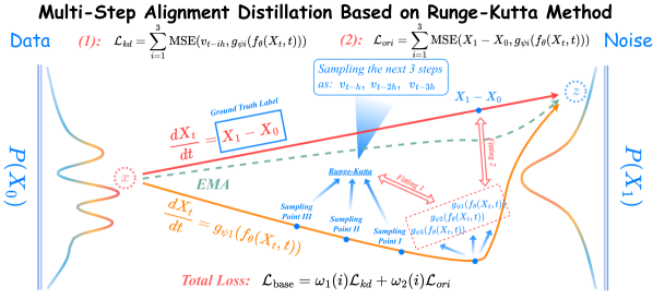
Figure 1: The framework of Runge-Kutta-based multi-step alignment distillation (Runge-Kutta 34).

• We present Catch-Up Distillation (CUD), the first accelerated sampling framework in a single training session without pre-training weights to extend the applicability of distillation-based accelerated sampling algorithms.

• We search the design space of CUD and obtain some suitable strategies based on experiments and theories, which allow for a significant improvement in the quality of the synthetic samples.

• We conduct extensive comparison and ablation experiments on the CIFAR-10, MNIST, and ImageNet-64 datasets to verify that CUD can achieve superior performance compared to the original DPM training, using the same number of iteration steps.

2 Background

Rectified flow.

It is well known that ODE-based training and sampling are conceptually simpler and require fewer Network Function Evaluations (NFEs) compared to those based on SDEs. Thus, in this work, we focus on ODE-based generative models and design a novel algorithm with the expectation that our CUD can be done in a single training session without the need for pre-trained weights, ultimately achieving accelerated sampling. Rectified flow [25] is a recent work that achieves ODE-based training by minimizing the transport cost between marginal distributions $\pi_{1}$ and $\pi_{0}$, i.e., $\mathbb{E}[c(X_{1}-X_{0})]$, where $X_{1}=\textrm{Law}(\pi_{1})$, $X_{0}=\textrm{Law}(\pi_{0})$ and $c:\mathbb{R}^{d}\rightarrow\mathbb{R}$ refers to a cost function. Due to the computational complexity of Optimal Transport (OT), Rectified flow provides a straightforward yet effective approach to generate a new coupling from a given one, which can be optimized using Stochastic Gradient Descent (SGD), a widely adopted optimization method in deep learning:

$$\theta^{*}=\operatorname*{arg\,max}_{\theta}\mathbb{E}_{t\sim\mathcal{U}[\epsilon,1]}\mathbb{E}_{X_{0},X_{1}\sim\pi_{0},\pi_{1}}[\lambda(t)\textrm{MSE}(X_{1}-X_{0}-f_{\theta}(X_{t},t))],$$ (1)

where $\lambda(t)$ and MSE refer to the weight function that satisfies $\lambda(t)\equiv 1$ and Mean Square Error (MSE), respectively. $\epsilon$ is a very small amount (i.e. 1e-5) to empirically avoid unnecessary fitting overhead. Furthermore, $X_{t}=tX_{1}+(1-t)X_{0}$ is chosen to ensure that $\forall f_{\theta}(X_{t},t)$ fits the same target velocity $X_{1}-X_{0}$. After training the sampling can be done by definite integral, i.e., $Z_{0}=Z_{1}+\int_{1}^{0}f_{\theta^{*}}(Z_{\tau},\tau)d\tau$, s.t., $Z_{1}=X_{1}$. Intuitively, we can utilize this ODE solution approach to gradually reduce noise in a “clean” image, and restore it to the original data distribution, denoted as $\pi_{0}$. In a series of well-established studies [27, 26, 38, 25, 17], numerical methods such as Euler’s method, Heun’s method, and Runge-Kutta method, have been effectively employed for solving ODEs in the sampling phase.

Reparameterized Noise Encoder.

Rectified flow employs a distillation technique to reduce transport costs by fitting $Z_{1}\!-\!Z_{0}$ instead of $X_{1}\!-\!X_{0}$. Commonly, this method requires an additional training phase. Do not like vanilla Rectified flow, in [23], the authors propose defining a reparameterized noise encoder $q_{\psi}(\widetilde{X}_{1}|X_{0})$ to reparameterize Gaussian noise, ensuring a smooth mapping from $X_{0}$ to $X_{1}$ and inducing efficient optimization. The new optimization objective can be expressed as

$$\operatorname*{arg\,max}_{\theta,\psi}\mathbb{E}_{t\sim\mathcal{U}[\epsilon,1]}\mathbb{E}_{\widetilde{X}_{1}=q_{\psi}(X_{0}),X_{0}\sim\pi_{0}}[\lambda(t)\textrm{MSE}(\widetilde{X}_{1}-X_{0}-f_{\theta}(X_{t},t))+\beta\textrm{D}_{KL}(q_{\psi}(\widetilde{X}_{1}|X_{0})||\pi_{1})].$$ (2)

Here, $\beta$ and $\textrm{D}_{KL}$ represent the loss weight (default as $20$) and Kullback-Leibler divergence, respectively. Although $q_{\psi}(z|x)$ is primarily designed to minimize the curvature on the transport path, we demonstrate that it also reduces transport costs empirically. We substantiate this through Theorem 2.1, which implies that as the Mutual Information (MI) between two distributions increases, the corresponding transport cost diminishes. Higher MI signifies a stronger correlation between the two probability distributions. This means that as long as the cost function chosen for training is inversely proportional to MI, we can observe a smaller transport cost between samples drawn from these distributions than without a reparameterized noise encoder.

Theorem 2.1.

(Proof in Appendix A) If the cost function $\mathbb{E}[c(a-b)]\propto 1/I(\textrm{Law}(a),\textrm{Law}(b))$, where $a$ and $b$ are samples drawn from any pair of marginal distributions, then the transportation cost between $\textrm{Law}(\widetilde{X}_{1})$ and $\textrm{Law}({X}_{0})$ is smaller than the transportation cost between $\textrm{Law}({X}_{1})$ and $\textrm{Law}({X}_{0})$.

With the above analysis in mind, we will take the optimization objective 2 as a baseline and explore how to utilize distillation for accelerating sampling.

Knowledge Distillation in Accelerating Sampling.

Knowledge distillation is an effective technique for compressing models that can enhance the generalization ability of lightweight models. While distillation is commonly used to compress models, it can also accelerate the sampling process of DPMs. The studies of [36, 29][42][28, 40] compress the multi-step sampling process of the DPM into a single step, effectively reducing computational overhead without compromising the quality of the synthetic images. However, these algorithms require pre-trained weights, and the student architecture is heavily dependent on the selected teacher architecture, limiting their scalability. In this paper, we aim to enable a DPM to function as both a teacher and a student, and accelerate sampling within a single training session without requiring any pre-trained weights, as compared to the above-mentioned work. It means that CUD can be considered a standard training session for DPMs with some additional loss terms, therefore ensuring its good portability.

3 Methodology

The conventional training objective for ODE/SDE-based generative models is to take input samples $X_{t}$ at different time points $t$ and output the noise $X_{1}$, sample $X_{0}$, or velocity $X_{1}\!-\!X_{0}$, aligning them with the corresponding ground truth labels. This paradigm is incapable of allowing the model to generate high-quality samples in a few sampling steps scenario. Although Song et.al. propose Consistency Training (CT), the method is only applicable to empirical PF ODE [40] since it needs Karra’s diffusion model paradigm [17] for supervision (detailed explanation can be found in Appendix B) and has a huge performance gap compared to their proposed Consistency Distillation (CD). These shortcomings prevent CT from generalizing to other diffusion model paradigms, e.g., VP-SDE, VE-SDE. Considering this issue, our proposed Catch-Up Distillation (CUD) aims to adjust the original training paradigm so that it not only performs ground truth label alignment but also enables $f_{\theta}(X_{t},t)$ “catch up” with the output from catch-up sampling. The term “catch-up sampling” refers to using a numerical integral solver to estimate $\widetilde{X}_{t-h}$ from $X_{t}$, where “$h$” refers to the step size of the discrete sampling. As presented in Fig. 1, CUD leverages Runge-Kutta-based multi-step alignment distillation for achieving accelerated sampling. Particularly, CUD also includes a series of simple but effective strategies (e.g. use the training model for catch-up sampling, random step size, dynamic skip connection) derived from searching the design space. Ultimately, the procedures of the CUD algorithm using Runge-Kutta 12, 23, and 34 are presented in Algorithms 3, C and C, respectively. Algorithms C and C and CUD’s limitations and broader impact can be found in the Appendix E and H.

Algorithm 1 ²  The Training Procedure of Catch-Up Distillation (Runge-Kutta 12)

1:procedure CUD($f_{\theta}$,$g_{\psi 1}$, $X_{0}\sim\pi_{0}$, $N\left(=50w\right)$, $\hat{h}=(1/16)$, $\alpha=(0.9999)$, $\epsilon=(1e\!-\!5)$, $\eta=(2e\!-\!4)$)

2:    Initialize $\theta_{-}\leftarrow\theta$, $\psi 1_{-}\leftarrow\psi 1$ $\triangleright$ Initialize the EMA model

3:    for $i\in\{1,\dots,N\}$ do$\triangleright$ Perform N iterations of training

4:        sample $t\sim\mathcal{U}[\epsilon,1]$, $h\sim\mathcal{U}[\epsilon,\hat{h}]$ $\triangleright$ Sampling time point and catch-up step size

5:        reparameter $X_{1}\leftarrow q_{\psi}(X_{0})$, compute $X_{t}\leftarrow tX_{1}+(1-t)X_{0}$ $\triangleright$ Generate sample point $X_{t}$

6:        $v_{t}\leftarrow g_{\psi 1}(f_{\theta}(X_{t},t))$ $\triangleright$ Calculate the velocity for the current time step

7:        if $t-h\geq\epsilon$ then $\triangleright$ Calculate the velocity for the next 1st time step

8:           $v_{t-h}\leftarrow g_{\psi 1}(f_{\theta}(\widetilde{X}_{t-h},t-h))$, $\widetilde{X}_{t-h}\leftarrow X_{t}-v_{t}h$ $\triangleright$ The right distillation behaviour

9:        else

10:           $v_{t-h}\leftarrow X_{1}-X_{0}$ $\triangleright$ Avoid the wrong distillation behaviour         

11:        $\mathcal{L}_{\textrm{prior}}=\beta\textrm{D}_{KL}(\textrm{Law}(X_{1})||\pi_{1})$ $\triangleright$ Let the marginal distribution of $X_{1}$ approximate $\mathcal{N}(0,\textbf{I})$

12:        $\mathcal{L}_{\textrm{base}}=\omega_{1}(i)\textrm{MSE}(v_{t-h},v_{t})+\omega_{2}(i)\textrm{MSE}(X_{1}-X_{0},v_{t})$ $\triangleright$ Our method’s core loss function

13:        $\theta\leftarrow\theta-\eta\nabla_{\theta}\mathcal{L}_{\textrm{CUD}},\ \psi 1\leftarrow\psi 1-\eta\nabla_{\psi 1}\mathcal{L}_{\textrm{CUD}},\ \psi\leftarrow\psi-\eta\nabla_{\psi}\mathcal{L}_{\textrm{CUD}}$, $\mathcal{L}_{\textrm{CUD}}=\mathcal{L}_{\textrm{prior}}+\mathcal{L}_{\textrm{base}}$

14:        update $\theta_{-}\leftarrow\alpha\theta_{-}+(1-\alpha)\theta,\psi 1_{-}\leftarrow\alpha\psi 1_{-}+(1-\alpha)\psi 1$$\triangleright$ Update based on EMA     

15:    return $\theta_{-},\psi 1_{-},\psi$ $\triangleright$ Return the model parameters

3.1 Basic Catch-Up Distillation

Integrating CD into continuous time steps may seem beneficial, but as demonstrated in Table 1 in our experiments, it can lead to training collapse. This issue arises because the Exponential Moving Average (EMA) model, $f_{\theta_{-}}(\cdot,\cdot)$, which guides training, may become unreliable due to inaccurate updates. We can derive Theorem 3.1 and thus simply explicate this fact.

Theorem 3.1.

(Proof in Appendix C) Assume that $\operatorname*{sup}_{X_{t}}L(f_{\theta}(X_{t},t),f_{\theta_{-}}(X_{t}-hf_{\Psi}(X_{t},t),t-h))\leq\gamma_{1}$ and $\operatorname*{sup}_{X_{t}}L(f_{\theta}(X_{t},t),f_{\theta_{-}}(X_{t},t))\leq\gamma_{2}$ after training convergence, where $L$, $\theta_{-}$, and $\Psi$ denote the norm, the parameters updated via EMA, and the pre-trained weight, respectively. And $f_{\theta}(\cdot,t)$ satisfies Lipschitz condition, i.e., $||f_{\theta}(x,t)-f_{\theta}(y,t)||\leq K||x-y||$, there exists $K>0$ such that for all $t\in[\epsilon,1]$. Then if $\epsilon\leq t_{a}\leq t_{b}\leq 1$ exists, we can obtain that

$$||f_{\theta}(X_{t_{b}},t_{b})-f_{\theta}(X_{t_{a}},t_{a})||\leq\frac{t_{b}-t_{a}}{h}\left[\gamma_{1}+\gamma_{2}+Kh||f_{\Psi}(X_{t_{b}},t_{b})-(X_{1}-X_{0})||\right],$$ (3)

The theorem establishes an upper bound, ensuring the stability of the distillation process. When the EMA model’s one-step update is inaccurate, $\gamma_{2}$ will become larger, leading CD to training collapse. It also implies that the difference between $f_{\Psi}(X_{t_{b}},t_{b})$ and $X_{1}-X_{0}$ must be adequately small for the process to remain stable. In the standard diffusion model training session, we do not have a pre-trained weight like CD, so we have to replace $\Psi$ with $\theta$. In line with common distillation algorithms, such as vanilla KD [13], RKD [32], and HSAKD [3], the teacher model output and the ground truth label mutually supervise the student model output. This approach enhances the student model’s generalization ability empirically. Consequently, we introduce a ground truth label to enable effective supervision, thereby avoiding the EMA model’s misdirected guidance. The output of $f_{\theta}(X_{t},t)$, for all $t\in[\epsilon,1]$, should align with $X_{1}-X_{0}$. We term this minimal functional algorithm as basic CUD, which synchronizes the ground truth label while “catches up” to the model output at the previous moment. Thus, the new base loss can be denoted as

$$\mathcal{L}_{\textrm{base}}=\mathbb{E}_{t\sim\mathcal{U}[\epsilon,1]}\mathbb{E}_{\widetilde{X}_{1}=q_{\psi}(X_{0}),X_{0}\sim\pi_{0}}[\omega_{1}(i)L(\widetilde{X}_{t-h},f_{\theta}(X_{t},t))+\omega_{2}(i)L(\widetilde{X}_{1}-X_{0},f_{\theta}(X_{t},t))],$$ (4)

where $X_{t}=t\widetilde{X}_{1}+(1-T)X_{0}$ and $\widetilde{X}_{t-h}$ is calculated by catch-up sampling using ODE $\frac{dX_{t}}{dt}=f_{\theta_{-}}(X_{t},t)$. And $\omega_{1},\omega_{2}$ represent the loss weights, which can even be parameterized by the number of current iterations, i.e., dynamic weight in Table 1.

3.2 Runge-Kutta-Based Multi-Step Alignment Distillation

One of the key components of our CUD is catch-up sampling, which can be solved by different ODE solvers. Notably, Euler’s method and Heun’s method are the subsets of Runge-Kutta methods, w.r.t., Runge-Kutta 12, and Runge-Kutta 23. So in this study, we apply Runge-Kutta methods to model catch-up sampling on a generic perspective. We only consider the Runge-Kutta algorithm up to order 3, as higher-order algorithms would lead to excessive computational overhead, even though it is possible to ignore the backpropagation of gradients and parameter updates by means of inference’s form, e.g., torch.no_grad(). In general, the points sampled

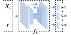
Figure 2: The architecture of the velocity estimation model with various heads.

by the higher-order Runge-Kutta will only serve for one sampling step. But this format obviously wastes a very large amount of training overhead, so is it possible to make the best use of all the sampling points? The answer is yes, as shown in Fig. 1. We can achieve Runge-Kutta-based multi-step alignment distillation, which aims to give the next step, the next-next step and even the next-next-next step of the estimated velocities simultaneously through all available sampling points, and then align them with outputs of different heads $\{g_{\psi i}(\cdot)\}_{i=1}^{n}$, where $n$ refers to the order of the Runge-Kutta method. Note that $g_{\psi 1}(f_{\theta}(\cdot,\cdot))$ on here is equivalent to $f_{\theta}(\cdot,\cdot)$ as mentioned earlier. As illustrated in Fig. 2, the input of all heads is the output of $f_{\theta}(\cdot,\cdot)$, and all heads are single meta-encoders that can be modeled as the sequence of consecutive GroupNorm-SiLU-Conv. By derivation in Appendix D, we can derive Runge-Kutta (23/34)-based multi-step alignment distillation as follows:

$$k_{1}=g_{\psi 1}(f_{\theta}(X_{t},t)),k_{2}=g_{\psi 1}(f_{\theta}(X_{t}-hk_{1},t-h)),$$

$$\widetilde{X}_{t-h}=X_{t}-[\frac{1}{2}hk_{1}+\frac{1}{2}hk_{2}],\widetilde{X}_{t-2h}=X_{t}-[hk_{1}+hk_{2}],$$

$$v_{t-h}=g_{\psi 1}(f_{\theta}(\widetilde{X}_{t-h},t-h)),v_{t-2h}=g_{\psi 1}(f_{\theta}(\widetilde{X}_{t-2h},t-2h)),$$

$$\mathcal{L}_{\textrm{base}}=\omega_{1}(i)\sum_{i=1}^{2}\textrm{MSE}(v_{t-ih},g_{\psi i}(f_{\theta}(X_{t},t)))+\omega_{2}(i)\sum_{i=1}^{2}\textrm{MSE}(\widetilde{X}_{1}-X_{0},g_{\psi i}(f_{\theta}(X_{t},t))),\quad{\color[rgb]{0.839216,0.152941,0.156863}\#\textrm{Runge-Kutta 23}}$$

$$k_{1}=g_{\psi 1}(f_{\theta}(X_{t},t)),k_{2}=g_{\psi 1}(f_{\theta}(X_{t}-hk_{1},t-h)),k_{3}=g_{\psi 1}(f_{\theta}(X_{t}-\frac{7}{4}hk_{1}-\frac{1}{4}hk_{2},t-2h)),$$ (5)

$$\widetilde{X}_{t-h}\!=\!X_{t}\!-\![\frac{5}{12}hk_{1}\!+\!\frac{2}{3}hk_{2}\!-\!\frac{1}{12}hk_{3}],\widetilde{X}_{t-2h}\!=\!X_{t}\!-\![\frac{5}{6}hk_{1}\!+\!\frac{4}{3}hk_{2}\!-\!\frac{1}{6}hk_{3}],\widetilde{X}_{t-3h}\!=\!X_{t}\!-\![\frac{5}{4}hk_{1}\!+\!2hk_{2}\!-\!\frac{1}{4}hk_{3}],$$

$$v_{t-h}=g_{\psi 1}(f_{\theta}(\widetilde{X}_{t-h},t-h)),v_{t-2h}=g_{\psi 1}(f_{\theta}(\widetilde{X}_{t-2h},t-2h)),v_{t-3h}=g_{\psi 1}(f_{\theta}(\widetilde{X}_{t-3h},t-3h)),$$

$$\mathcal{L}_{\textrm{base}}=\omega_{1}(i)\sum_{i=1}^{3}\textrm{MSE}(v_{t-ih},g_{\psi i}(f_{\theta}(X_{t},t)))+\omega_{2}(i)\sum_{i=1}^{3}\textrm{MSE}(\widetilde{X}_{1}-X_{0},g_{\psi i}(f_{\theta}(X_{t},t))),\quad{\color[rgb]{0.839216,0.152941,0.156863}\#\textrm{Runge-Kutta 34}}$$

Compared to a simple one-step alignment distillation, the use of multi-step alignment distillation provides more comprehensive information about $\frac{X_{t}}{dt}=g_{\psi 1_{-}}(f_{\theta_{-}}(X_{t},t))$, resulting in preventing asynchronous model updates and improving model performance.

3.3 Investigate Design Space

To some extent, the basic CUD has facilitated accelerated sampling; however, further enhancements are feasible. In this subsection, we delineate the design space and conduct a comprehensive analysis, ultimately proposing strategies superior to the basic CUD.

Limitations of Using EMA Model in Catch-Up Sampling.

The update of the EMA model can enhance the model’s generalization ability. Nevertheless, during the training phase, the disparity between the parameters of the EMA model and the training model may cause the upper bound of Theorem 3.1 to be excessively loose, particularly in relation to the term $\gamma_{2}$ (as concluded in Appendix C). A more sensible and effective approach is to discard the EMA model and utilize the training model directly for catch-up sampling. In this case, the errors introduced by the incorrect estimation of the EMA model will no longer exist, further improving the performance of the model.

Random Step Size in Catch-Up Sampling.

For accelerating sampling, a large interval between sample points is employed to reduce the sample count. However, in widely-used diffusion models such as DDPM [15], NCSN [39], and Rectified flow, the interval between sampling points approaches zero, as these models necessitate accurate estimation of differential equations to prevent training collapse. Intuitively, utilizing a fixed value of $h$ for CUD may result in the model converging to suboptimal solutions. This occurs because, for $X_{t}$, the model can only obtain the solution in the time point $t-h$ and is unable to explore solutions in other time points that could provide a more precise estimate of the ODE. To tackle this problem, we implement a non-fixed-step size strategy, uniform, implying that the new step size $h$ follows a uniform distribution $\mathcal{U}[\epsilon,\hat{h}]$ ($\hat{h}$ is a predetermined step size, defaulting to 1/16). Additionally, we introduce a strategy named rule, which determines the new step size as $h=t\hat{h}$, aiming to ensure the quality of the synthetic image retains a degree of ambiguity when $t\rightarrow 1$, necessitating a larger step size to augment the distillation strength. Conversely, when

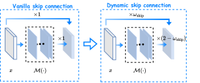
Figure 3: The overview of vanilla skip connection and dynamic skip connection.

$t\rightarrow\epsilon$, the synthetic image’s quality is superior, thus requiring a smaller step size to maintain stability.

Dynamic Skip Connection.

Training a velocity estimation model with a fixed architecture directly would be far from ideal. As demonstrated in Appendix F, the cost of fitting the training model varies at different $t$. In past work [17, 39, 31], they both apply a special operation that skips the entire model with residual mapping, i.e., $c_{\textrm{skip}}(t)X_{t}+c_{\textrm{out}}(t)(X_{t},t)$, where $c_{\textrm{skip}}(t)$ and $c_{\textrm{out}}(t)$ are two functions that input $t$ and output a scalar. However, this skip connection is coarse-grained and does not take advantage of the skip connection that contemporary mainstream neural networks [10, 11, 5, 34] have themselves. A slight modification to the original UNet, i.e., implementing dynamic weights on the vanilla skip connection, allows for a reasonable allocation of the fitting overhead of the loss function at different $t$, and can improve DPM’s performance simply and effectively. As shown in Fig. 3, we implement dynamic skip connection by a simple linear dynamic weight $\omega_{\textrm{skip}}$. Thus, the novel dynamic skip connection can be denoted as

Table 1: Basic CUD: only apply Runge-Kutta 12 and do not make use of strategies introduced in Sec. 3.3; RF: Rectified flow; vanilla weight: $\omega_{1}(i)\equiv 1$, $\omega_{2}(i)\equiv 1$; dynamic weight: $\omega_{1}(i)=i/N$, $\omega_{2}(i)=1-i/N$. The second column on the right represents the ODE solver and the number of sampling steps used. For example, “Euler, 4” represents the application of Euler’s method with 4 steps for sampling. The results of IS and other loss functions are presented in Table 6 and 7 in Appendix.

Methods		RF (Eq. 2)	CD (train based on RF under continuous time steps scenarios)			Basic CUD
Settings		MSE	MSE, $h\rightarrow 0$	MSE, $h\!=\!1/16$	LPIPS,$h\!=\!1/16$	MSE,$h\!=\!1/16$,	LPIPS,$h\!=\!1/16$,	MSE,$h\!=\!1/16$,	LPIPS,$h\!=\!1/16$,
						vanilla weight	vanilla weight	dynamic weight	dynamic weight
FID	Euler, 4	37.05	32.57	417.36	471.47	5.20	446.45	171.88	438.21
	Euler, 16	6.85	6.36	413.11	476.98	13.96	444.98	188.99	434.61
	Heun, 4	13.58	12.88	414.23	477.17	6.28	445.31	195.27	434.43
	Heun, 16	4.15	4.43	407.84	473.55	17.62	444.48	193.47	433.10

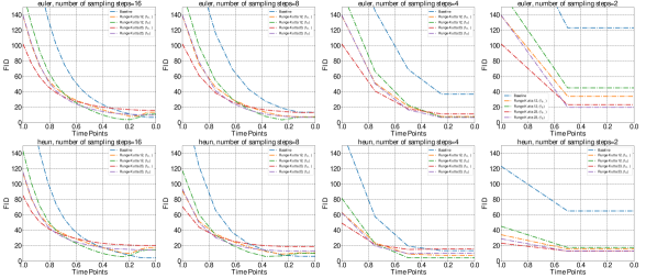
Figure 4: Ablation experiments on whether to use the EMA model for CUD.

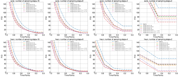
Figure 5: Ablation experiments on whether to use the random step size and dynamic skip connection for CUD.

$$x_{o}=\omega_{\textrm{skip}}x+(2-\omega_{\textrm{skip}})\mathcal{M}(x),$$ (6)

where $x$, $x_{o}$, and $\mathcal{M}(\cdot)$ refer to the input, output, and intermediate layers, respectively. Furthermore, $\omega_{\textrm{skip}}=2(1-(t(1-2c_{\textrm{skip}})+c_{\textrm{skip}}))$ is an equation where $c_{\textrm{skip}}$ is a pre-set hyperparameter that we choose as either 0.25 or 0.75. Notably, we replace all vanilla skip connections in UNet with dynamic skip connections.

4 Experiment

We conduct experiments to evaluate the effectiveness of CUD on CIFAR-10 [22] with a resolution of 32$\times$32, excluding the comparison experiments. We use three datasets for the comparison experiments: CIFAR-10 with resolution 32$\times$32, MNIST with resolution 28$\times$28, and ImageNet-64 with resolution 64$\times$64. We assess the quality of the synthetic samples using Fréchet Inception Distance (FID) [12] and Inception Score (IS) [37]. To compute the FID, we compare 50,000 synthetic samples with all available real samples, and for computing the IS, we used 50,000 synthetic samples. We employed 4 different configurations for the velocity estimation model and hyperparameters on CIFAR-10, MNIST, and ImageNet-64. Specifically, we used configurations (a), (b), and (c) to train DPMs on CIFAR-10, MNIST, and ImageNet-64, respectively, and configuration (d) for our proposed final multi-step distillation (see Appendix G) on all datasets. The implementation details for these settings are provided in Appendix J. Unless otherwise specified, configuration (a) was used for ablation studies and analyses.

4.1 Ablation Study

Basic CUD.

To verify that the basic CUD is capable of accelerated sampling, we conduct experiments and present the results in Table 1. In this table, the dynamic weight represents the supervision focus during training. At the beginning of the training, dynamic weight emphasizes using the ground truth label for supervision. In contrast, at the end of the training, dynamic weight emphasizes using the output of the teacher model for supervision. And $L$ is one of Learned Perceptual Image Patch Similarity (LPIPS) [46] and MSE. LPIPS is more effective than MSE in Consistency Model [40]. But according to Table 1, we can conclude that MSE can work, but LPIPS does not, and that vanilla weight can work but dynamic weight does not. Meanwhile, the effective choice of loss function $L$, as well as the loss weights $\omega_{1}$ and $\omega_{2}$ in the basic CUD, are MSE, $\omega_{1}(i)\equiv 1$, and $\omega_{2}(i)\equiv 1$, respectively.

Investigate Design Space.

We present experimental results in Figs. 4 and 5 to assess the efficacy of our proposed suitable strategies. In these figures, Runge-Kutta 12/23 represents the form utilized in Runge-Kutta-based multi-step alignment distillation, while $f_{\theta_{-}}$ and $f_{\theta}$ denote the employment of the EMA model and the training model for catch-up sampling, respectively. Here, we do not consider the ground truth loss terms $\textrm{MSE}(\widetilde{X}_{1}-X_{0},g_{\psi 2}(f_{\theta}(X_{t},t)))$ and $\textrm{MSE}(\widetilde{X}_{1}-X_{0},g_{\psi 3}(f_{\theta}(X_{t},t)))$. In Appendix I, we perform ablation experiments to show their importance. For all intermediate sampling points, we employ velocity estimation using a one-step method to synthetic samples. Specifically, when obtaining an intermediate sampling point $Z_{m}$, we calculate the target “clean” image $Z_{0}$ using $Z_{0}=Z_{m}-mf_{\theta}(Z_{m},m)$ (Euler’s method). From Fig. 4, we deduce that employing the training model for catch-up sampling is more beneficial than using the EMA model, suggesting the application of $f_{\theta}$ instead of $f_{\theta_{-}}$ in Eq. 4. CUD is more effective in scenarios with fewer sampling steps but may be less effective than the baseline when more sampling steps are present. This is because CUD’s primary purpose is to accelerate sampling rather than improve the quality of synthetic images. Consequently, the velocity estimation model should prioritize generating “clean” images in scenarios with fewer sampling steps rather than enhancing image quality in scenarios with more sampling steps. Additionally, in Fig. 5, we observe that both uniform and rule surpass the baseline in terms of synthetic image quality in nearly all scenarios, with greater improvements seen with fewer sampling steps. In fewer sampling steps scenarios, rule outperforms uniform, while the opposite is true for scenarios with more sampling steps (details are provided in Appendix K). Notably, uniform achieves the best CUD performance, with an FID of 3.36. Lastly, the ablation experiments on dynamic skip connections are also presented in Figs. 5. Both $c_{\textrm{skip}}=$0.25 and $c_{\textrm{skip}}=$0.75 work very well because the fitting cost is minimized when $t$ is close to 0.5. In particular, $c_{\textrm{skip}}=$0.75 performs better than $c_{\textrm{skip}}=$0.25, achieving an FID 2.91 in 15 steps of sampling (see Appendix K). This suggests that to improve the quality of the synthetic images, the model should focus more on enhancing the representation at $t\rightarrow 0$ rather than $t\rightarrow 1$. By combining the above three suitable strategies that require no additional overhead and are simple yet effective, the best performance of CUD on FID has decreased from 5.20 (4 steps to sampling with Heun’s method) to 2.91 (15 steps to sampling with Euler’s method).

Runge-Kutta-Based Multi-Step Alignment Distillation.

We perform ablation studies to assess the efficacy of Runge-Kutta-based multi-step alignment distillation across different orders, specifically utilizing the CIFAR-10 and MNIST datasets. The corresponding results are displayed in Tables 3 and 3. When examining the performance of Runge-Kutta orders 12, 23, and 34 on CIFAR-10, it becomes evident that images produced by Runge-Kutta 23 yield the most desirable performance. However, Runge-Kutta 34 attains the greatest accelerated sampling effect, followed by Runge-Kutta 23 and 12. In contrast, for the MNIST dataset, Runge-Kutta 34 provides the best performance and the most effective accelerated sampling. These empirical findings suggest that the accelerated sampling effect intensifies with the increase in the order of Runge-Kutta-based multi-step alignment distillation. Although the quality of images generated by Runge-Kutta 34 on CIFAR-10 is not as optimal as those produced by Runge-Kutta 12 and 23, it is justified due to the higher complexity of CIFAR-10 compared to MNIST, and the greater emphasis placed by Runge-Kutta 34 on improving accelerated sampling rather than enhancing the quality of the synthetic images.

Table 2: Experimental results on CIFAR-10. ^∗Apply our proposed final multi-step distillation.

    METHOD Solver NFE ($\downarrow$) FID ($\downarrow$) IS ($\uparrow$) Generative Adversarial Network (GAN)   BigGAN [2] - 1 14.7 9.22 AutoGAN [7] - 1 12.4 8.55 StyleGAN [16] - 1 8.32 9.18 StyleGAN+ADA [16] - 1 2.92 9.40 Diffusion Model (One Session)   DDPM [15] - 1000 3.21 9.46 DDPM DDIM [38] 10 8.23 - DDPM DPM-solver-2 [27] 12 5.28 - DDPM DPM-solver-3 12 6.03 - NCSN++ [41] Euler-Maruyama 2000 2.38 9.83 1-Rectified Flow⁺ [25] Runge-Kutta 45 127 2.58 9.60 2-Rectified Flow⁺ Runge-Kutta 45 110 3.36 9.24 Curvature⁺ [23] Euler 16 6.85 8.84 Curvature⁺ Euler 4 37.05 7.07 Curvature⁺ Heun 7 13.58 8.49 CUD (Runge-Kutta 12)⁺ Euler 15 2.91 9.90 CUD (Runge-Kutta 12)⁺ Euler 4 17.40 9.38 CUD (Runge-Kutta 12)⁺ DPM-solver-2 4 8.25 8.95 CUD (Runge-Kutta 23)⁺ Euler 15 2.80 9.36 CUD (Runge-Kutta 23)⁺ Euler 4 12.23 8.39 CUD (Runge-Kutta 23)⁺ DPM-solver-2 4 6.42 8.90 CUD (Runge-Kutta 34)⁺ Euler 14 3.40 9.39 CUD (Runge-Kutta 34)⁺ Euler 4 9.45 8.50 CUD (Runge-Kutta 34)⁺ Heun 7 4.70 9.34 Diffusion Model (Two Session)   2-Rectified Flow+(distillation)⁺ Euler 110 4.85 9.01 PD [36] DDIM 1 8.34 8.69 PD DDIM 2 5.58 9.05 CD [40] Karra’s method [17] 1 3.55 9.48 CD Karra’s method 2 2.93 9.75 CUD (Runge-Kutta 12)+(distillation)^∗+ Euler 1 3.37 9.42 CUD (Runge-Kutta 23)+(distillation)^∗+ Euler 1 3.76 9.34 CUD (Runge-Kutta 34)+(distillation)^∗+ Euler 1 4.44 9.09  

Table 3: Experimental results on MNIST and ImageNet-64. ⁺Train based on Rectified flow.

    METHOD Solver NFE ($\downarrow$) FID ($\downarrow$) IS ($\uparrow$) MNIST (One Session)   1-Rectified flow⁺ [25] Euler 4 31.67 1.95 1-Rectified flow⁺ [25] Euler 16 11.16 2.06 1-Rectified flow⁺ [25] Runge-Kutta 45 41 10.77 2.10 Curvature⁺ [23] Euler 16 21.77 2.11 Curvature⁺ Euler 4 49.96 2.02 Curvature⁺ Heun 7 21.55 2.10 CUD (Runge-Kutta 12)⁺ Euler 16 3.39 2.01 CUD (Runge-Kutta 12)⁺ Euler 4 9.45 2.02 CUD (Runge-Kutta 23)⁺ Euler 16 2.18 2.10 CUD (Runge-Kutta 23)⁺ Euler 4 7.06 2.03 CUD (Runge-Kutta 34)⁺ Euler 16 1.81 2.10 CUD (Runge-Kutta 34)⁺ Euler 4 6.70 2.03 MNIST (Two Session)   PD⁺ [36] Euler 2 9.60 2.11 CD⁺ [40] Euler 2 8.96 2.05 CUD (Runge-Kutta 12)+(distillation)⁺ Euler 1 8.94 2.08 CUD (Runge-Kutta 12)+(distillation)^∗+ Euler 1 6.38 2.12 CUD (Runge-Kutta 23)+(distillation)^∗+ Euler 1 3.08 2.08 CUD (Runge-Kutta 34)+(distillation)^∗+ Euler 1 5.43 2.09       METHOD Solver NFE ($\downarrow$) FID ($\downarrow$) Prec. ($\uparrow$) ImageNet-64 (One Session)   BigGAN-deep [2] - 1 4.06 0.79 IDDPM (small) - 4000 6.92 0.77 IDDPM (large) - 4000 2.92 0.82 ADM DDIM 250 2.61 0.73 ADM (dropout) DDIM 250 2.07 0.74 EDM Karra’s method 79 2.44 0.71 U-ViT-M/4 DPM-solver-2 50 5.85 - U-ViT-L/4 DPM-solver-2 50 4.26 - CUD (Runge-Kutta 12)⁺ Euler 4 18.84 0.58 CUD (Runge-Kutta 12)⁺ Euler 8 7.75 0.68 CUD (Runge-Kutta 12)⁺ Euler 16 5.05 0.71 CUD (Runge-Kutta 12)⁺ DPM-solver-2 6 7.68 0.68  

4.2 Comparison Experiments

The comparative experiments are performed on CIFAR-10, MNIST, and ImageNet-64 to highlight the performance benefits of CUD. The results of PD [36], CD [40], and Curvature [23] algorithms on MNIST are derived from Rectified flow, as the results of these methods are available for analysis. The relevant experimental results are presented in Tables 3 and 3, and the remaining supplementary results are given in Appendix I. Considered as a one-session training approach, we first compare CUD with other one-session training methods, such as the train-free accelerated sampling techniques, namely “DPM-solver” and DDIM, as well as a variety of DPMs, specifically NCSN++, DDPM, Rectified Flow, and Curvature, which serves as the baseline. For experiments on all datasets, CUD is very effective in accelerating sampling. For instance, CUD achieves the best performance in the few-step image generation scenario. For instance, on CIFAR-10, a FID 4.70 obtained by a CUD (Runge-Kutta 34) sample in just 7 steps better than a FID 5.28 obtained by a DPM-solver-2 sample in 12 steps.

Moreover, for the two-session training scenario, since CUD is trained on a continuous time step, it suffers from performance limitations. This is largely attributed to the excessive number of time points required for fitting, making it slightly inferior to both PD and CD algorithms. To address this, we introduced a novel multi-step distillation algorithm that extends the distillation algorithm presented in [25], as a way to achieve one-step sampling. Specifically, the algorithm is designed to incrementally fit “clean” images obtained at different time steps (e.g., when t progresses from 1/2 to 5/16 to 1/8). The effectiveness of this approach has been validated through quantitative ablation experiments discussed in Appendix G. Leveraging this, we conduct distillation on the pre-trained model derived from CUD (Runge-Kutta 12), ultimately achieving a state-of-the-art FID of 3.37 by sampling in one step on CIFAR-10. Furthermore, our approach demonstrates cost-effectiveness in training, requiring only 620k (500k+120k) iterations on CIFAR-10 with a batch size of 128 and a model parameter number of 55M, compared to CD’s 2100k (1300k+800k) iterations with a batch size of 256 and a model parameter number of 62M. Performance-wise, on both MNIST and ImageNet-64, CUD demonstrates comparable results to PD and CD. Lastly, synthetic images generated by our approach can be found in Appendix L.

5 Conclusion

This paper presents Catch-Up Distillation (CUD), a method designed to integrate effortlessly with the existing diffusion model training paradigm, enabling high-quality image synthesis in fewer sampling steps, and eliminating the need for pre-training weights. The efficacy of CUD is substantiated through the validation of several datasets, including CIFAR-10, MNIST, and ImageNet-64. In subsequent research, we sincerely hope that our CUD can be extended to discrete time steps where only a small number of time points need to be fitted, thus further enhancing the generality of CUD.

Appendix A Transport Cost under Reparameterized Noise Encoder $p_{\psi}(\cdot)$

For a coupling $(X_{0},X_{1})$, where $X_{0}\sim\pi_{0},\ X_{1}\sim\pi_{1}$ and satisfies $p(\pi_{0},\pi_{1})=p(\pi_{0})p(\pi_{1})$, we have the Mutual Information (MI) between $\pi_{0}$ and $\pi_{1}$ is $0$, a.k.a., $I(\pi_{0},\pi_{1})=0$. Following [23], let us define a reparameterized noise encoder $q_{\psi}(\cdot)$ that satisfies $\widetilde{X}_{1}=q_{\psi}(X_{0})$ and $\min\textrm{D}_{KL}(q_{\psi}(\pi_{1}|\pi_{0})||p(\pi_{1}))$. When the cost function $\mathbb{E}[c(X_{0}-X_{1})]\propto 1/I(\textrm{Law}(X_{0}),\textrm{Law}(X_{1}))$, we have $\mathbb{E}[c(X_{0}-\widetilde{X}_{1})]\leq\mathbb{E}[c(X_{0}-X_{1})]$.

Proof.

$$\mathbb{E}[c(X_{0}-\widetilde{X}_{1})] =k/I(\textrm{Law}(X_{0}),\textrm{Law}(\widetilde{X}_{1}))$$ (7)

$$=k/\textrm{D}_{KL}(p(\pi_{0},\pi_{1})||p(\pi_{0})q_{\psi}(\pi_{1}|\pi_{0}))$$

$$\leq k/\textrm{D}_{KL}(p(\pi_{0},\pi_{1})||p(\pi_{0})p(\pi_{1}))$$

$$=k/I(\textrm{Law}(X_{0}),\textrm{Law}({X}_{1}))$$

$$=\mathbb{E}[c(X_{0}-{X}_{1})],$$

where $k\in\mathbb{R}^{+}$ denotes a constant. ∎

Appendix B Consistency Distillation and Consistency Training

Pseudo-code and implementation details of Consistency Distillation (CD) and Consistency Training (CT) can be found in paper https://arxiv.org/abs/2303.01469 and github link https://github.com/openai/consistency_models. Although Song et. al. state that CD is capable of implementing the new state-of-the-art FID 3.55 under the condition of a single NFE, there still are some constraints on this:

Constraint I.

CD and CT may not be effective for certain popular DPMs such as Rectified flow [25], NCSN++, and DDPM [41]. When CD or CT is applied to Rectified flow under the continuous time steps scenarios, it causes the training to collapse in our experiments (Table 1). This means that CD/CT requires Karra’s method under discrete time steps scenarios for it to work properly.

Constraint II.

CT can only be applied in empirical PF ODE because if the model design for estimating “clean image”, i.e., $c_{\textrm{skip}}(\cdot),c_{\textrm{out}}(\cdot)$, in the DPM is ignored, then it is equivalent to its not having the ground truth label for effective supervision. For CT in empirical PF ODE, it relies on $f_{\theta}(X_{t},t)=c_{\textrm{skip}}(t)X_{t}+c_{\textrm{out}}(t)F_{\theta}(X_{t},t)$ to achieve implicit supervision. To be specific, CT’s core loss function $||f_{\theta}(X_{t+h},t+h)-f_{\theta}(X_{t},t)||_{2}^{2}$ can be rewritten as $||c_{\textrm{skip}}(t+h)X_{t+h}-c_{\textrm{skip}}(t)X_{t}+c_{\textrm{out}}(t+h)F_{\theta}(X_{t+h},t+h)-c_{\textrm{out}}(t)F_{\theta}(X_{t},t)||_{2}^{2}$. Setting $X_{t}=X_{0}+tX_{1},\ X_{1}\sim\mathcal{N}(0,\mathbf{I})$, $c_{\textrm{skip}}(t)=1-t$ and $c_{\textrm{out}}(t)=t$, the loss function can continue to be rewritten as $||t(F_{\theta}(X_{t+h},t+h)-F_{\theta}(X_{t},t))+hF_{\theta}(X_{t+h},t+h)-h(X_{0}-(1-2t)X_{1})-h^{2}X_{1}||_{2}^{2}$. Since empirical PF ODE guarantees that $f_{\theta}(X_{t},t)$ is an identity function when $t=0$, i.e., $f_{\theta}(X_{0},0)=X_{0}$, $F_{\theta}(X_{t+h},t+h)$ is applied to fit the ground truth label $\frac{tF_{\theta}(X_{t},t)+hX_{0}+h(2t-1)X_{1}+h^{2}X_{1}}{t+h}$. If $t=0$, $f_{\theta}(X_{h},h)$ is required to fit $X_{0}+(h-1)X_{1}$. Then, if $t=h$, $f_{\theta}(X_{2h},2h)$ is required to fit $X_{0}+(2h-1)X_{1}$… Therefore, through a chain reaction, if $t=ih$, $f_{\theta}(X_{(i+1)h},(i+1)h)$ is required to fit $X_{0}+((i+1)h-1)X_{1}$.

Of course, this exquisite form of chain constraint accomplishes effective supervision, but it also hinders its possible application to other DPMs.

Constraint III.

Although the CT algorithm is able to accomplish distillation without relying on pre-trained weights for accelerating sampling, its application limitations and not very impressive performance prevent it from being a general-purpose algorithm. Our proposed CUD exists to address this problem, and it is theoretically applicable to any continuous SDE/ODE algorithm w.r.t., for SDE Runge-Kutta-based multi-step alignment distillation can be done with DDIM [38].

Constraint IV.

The models utilized in CD/CT, possessing 62 million parameters, are larger than our proposed CUD, which encompasses 55 million parameters in the CIFAR-10 dataset. CD requires 80w iterations for training, not including the additional 130w iterations necessary to train the original diffusion model. In contrast, CUD, despite incorporating multi-step distillation, only necessitates a total of 62w iterations, broken down into 50w and 12w iterations, respectively.

Appendix C The Working Principle of Base Loss $\mathcal{L}_{\textrm{base}}$

Before explaining why our proposed base loss can work, we first need to explain why Consistency Distillation (CD) of Consistency Model cannot work. As you know, the loss function of CD can be denoted as

$$\mathcal{L}_{\textrm{CT}}=L(f_{\theta}(X_{t},t),f_{\theta_{-}}(X_{t}-hf_{\Psi}(X_{t},t),t-h)),$$

where $L(\cdot,\cdot)\in\mathbb{R}^{+}$, $\theta_{-}$, and $\Psi$ denote a distance function, the parameters of the EMA model, and the parameters of the pre-trained model, respectively. Assume that $\operatorname*{sup}_{X_{t}}L(f_{\theta}(X_{t},t),f_{\theta_{-}}(X_{t}-hf_{\Psi}(X_{t},t),t-h))\leq\gamma_{1}$ and $\operatorname*{sup}_{X_{t}}L(f_{\theta}(X_{t},t),f_{\theta_{-}}(X_{t},t))\leq\gamma_{2}$ after training convergence. And $f_{\theta}(\cdot,t)$ satisfies Lipschitz condition, i.e., $||f_{\theta}(x,t)-f_{\theta}(y,t)||\leq K||x-y||$, there exists $K>0$ such that $\forall$ $t\in[\epsilon,1]$. We can expand $\operatorname*{sup}_{X_{t}}L(f_{\theta}(X_{t},t),f_{\theta_{-}}(X_{t}-hf_{\Psi}(X_{t},t),t-h))\leq\gamma_{1}$ as

$$\operatorname*{sup}_{X_{t}}L(f_{\theta}(X_{t},t),f_{\theta_{-}}(X_{t}-hf_{\Psi}(X_{t},t),t-h))\leq\gamma_{1}$$ (8)

$$=> \operatorname*{sup}_{X_{t}}L(f_{\theta}(X_{t},t),f_{\theta}(X_{t}-hf_{\Psi}(X_{t},t),t-h))-\operatorname*{sup}_{X_{t}}L(f_{\theta}(X_{t}-hf_{\Psi}(X_{t},t),t-h),f_{\theta_{-}}(X_{t}-hf_{\Psi}(X_{t},t),t-h))\leq\gamma_{1}$$

$$=> \operatorname*{sup}_{X_{t}}L(f_{\theta}(X_{t},t),f_{\theta}(X_{t}-hf_{\Psi}(X_{t},t),t-h))\leq\gamma_{1}+\gamma_{2}$$

$$=> L(f_{\theta}(X_{t},t),f_{\theta}(X_{t-h},t-h))\leq L(f_{\theta}(X_{t-h},t-h),f_{\theta}(X_{t}-hf_{\Psi}(X_{t},t),t-h))+\gamma_{1}+\gamma_{2}.$$

Suppose that $L(\cdot,\cdot)$ is a norm, i.e., $||\cdot-\cdot||$. Then we can continue to derive Eq. 8 as

$$||f_{\theta}(X_{t},t)-f_{\theta}(X_{t-h},t-h)||\leq Kh||X_{1}-X_{0},f_{\Psi}(X_{t},t)||+\gamma_{1}+\gamma_{2}.$$ (9)

$\forall t_{a},t_{b}\in[\epsilon,1]$ satisfy $\epsilon\leq t_{a}\leq t_{b}\leq 1$, we have

$$||f_{\theta}(X_{t_{b}},t_{b})-f_{\theta}(X_{t_{a}},t_{a})||\leq\frac{t_{b}-t_{a}}{h}\left[\gamma_{1}+\gamma_{2}+Kh||f_{\Psi}(X_{t_{b}},t_{b})-(X_{1}-X_{0})||\right].$$ (10)

The right half of the above equation contains three terms: $\gamma_{1}$, $\gamma_{2}$, and $Kh||f_{\Psi}(X_{t_{b}},t_{b})-(X_{1}-X_{0})||$. Only these terms are small enough to ensure the stability of the distillation. CD ignores the difference $\gamma_{2}$ between the EMA model and the training model, which causes the training to collapse extremely easily under continuous time steps scenarios, especially if the EMA model is not updated accurately at one step.

If changing the pre-trained weight $\Phi$ to $\theta$, the left-hand side of Eq. 10 can be used directly to complete the distillation process. This form is different from the standard DPM training and is already widely applied in other applications to a certain extent. In image classification tasks, distillation algorithms typically involve two core losses: (1) Cross-Entropy loss between the student model output and the ground truth label, and (2) Kullback-Leibler Divergence between the student model output and the teacher model output. Collaborative supervision between the teacher model output and the ground truth label significantly enhances the generalization ability of the student model. This approach can also be applied to the DPM for distillation without teacher weights, thus achieving better performance of the student model.

Therefore, a distance function in the form of a norm as a loss function and the application of the ground truth label for supervision is necessary for the DPM. Only by ensuring these two points, Eq. 10’s bound does not collapse into training by being too lenient.

Algorithm 2 ²  The Training Procedure of Catch-Up Distillation (Runge-Kutta 23)

1:procedure CUD($f_{\theta}$,$\{g_{\psi i}\}_{i=1}^{2}$, $X_{0}\sim\pi_{0}$, $N\left(=50w\right)$, $\hat{h}=(1/16)$, $\alpha=(0.9999)$, $\epsilon=(1e\!-\!5)$, $\eta=(2e\!-\!4)$)

2:    Initialize $\theta_{-}\leftarrow\theta$, $\{\psi j_{-}\leftarrow\psi j\}_{j=1}^{2}$ $\triangleright$ Initialize the EMA model

3:    for $i\in\{1,\dots,N\}$ do$\triangleright$ Perform N iterations of training

4:        sample $t\sim\mathcal{U}[\epsilon,1]$, $h\sim\mathcal{U}[\epsilon,\hat{h}]$ $\triangleright$ Sampling time point and catch-up step size

5:        reparameter $X_{1}\leftarrow q_{\psi}(X_{0})$, compute $X_{t}\leftarrow tX_{1}+(1-t)X_{0}$ $\triangleright$ Generate sample point $X_{t}$

6:        $v_{t}^{1}\leftarrow g_{\psi 1}(f_{\theta}(X_{t},t))$, $v_{t}^{2}\leftarrow g_{\psi 2}(f_{\theta}(X_{t},t))$ $\triangleright$ Calculate the velocity for $g_{\psi 1}$, $g_{\psi 2}$

7:        $v_{t-h}^{\textrm{tmp}}\leftarrow g_{\psi 1}(f_{\theta}(X_{t}-v_{t}^{1}h,t-h))$

8:         $\triangleright$ Calculate the intermediate variables required by Runge-Kutta

9:        if $t-2h\geq\epsilon$ then $\triangleright$ Calculate the velocity for the next 1st and 2nd time step

10:           $\widetilde{X}_{t-2h}\leftarrow X_{t}-(v_{t}^{1}+v_{t-h}^{\textrm{tmp}})h$, $\widetilde{X}_{t-h}\leftarrow X_{t}-\frac{v_{t}^{1}+v_{t-h}^{\textrm{tmp}}}{2}h$ $\triangleright$ The right distillation behaviour

11:           $v_{t-2h}\leftarrow g_{\psi 1}(f_{\theta}(\widetilde{X}_{t-2h},t-2h))$, $v_{t-h}\leftarrow g_{\psi 1}(f_{\theta}(\widetilde{X}_{t-h},t-h))$

12:        else

13:           $v_{t-2h}\leftarrow X_{1}-X_{0}$, $v_{t-h}\leftarrow X_{1}-X_{0}$$\triangleright$ Avoid the wrong distillation behaviour         

14:        $\mathcal{L}_{\textrm{prior}}=\beta\textrm{D}_{KL}(\textrm{Law}(X_{1})||\pi_{1})$ $\triangleright$ Let the marginal distribution of $X_{1}$ approximate $\mathcal{N}(0,\textbf{I})$

15:        $\mathcal{L}_{\textrm{base}}=\omega_{1}(i)\sum_{j=1}^{2}\textrm{MSE}(v_{t-jh},v_{t}^{j})+\omega_{2}(i)\sum_{j=1}^{2}\textrm{MSE}(X_{1}-X_{0},v_{t}^{j})$

16:         $\triangleright$ Our method’s core loss function

17:        $\mathcal{L}_{\textrm{CUD}}=\mathcal{L}_{\textrm{prior}}+\mathcal{L}_{\textrm{base}}$

18:        $\theta\leftarrow\theta-\eta\nabla_{\theta}\mathcal{L}_{\textrm{CUD}},\ \{\psi j\leftarrow\psi j-\eta\nabla_{\psi j}\mathcal{L}_{\textrm{CUD}}\}_{j=1}^{2},\ \psi\leftarrow\psi-\eta\nabla_{\psi}\mathcal{L}_{\textrm{CUD}}$

19:        update $\theta_{-}\leftarrow\alpha\theta_{-}+(1-\alpha)\theta,\{\psi j_{-}\leftarrow\alpha\psi j_{-}+(1-\alpha)\psi j\}_{j=1}^{2}$$\triangleright$ Update based on EMA     

20:    return $\theta_{-},\{\psi j_{-}\}_{j=1}^{2},\psi$ $\triangleright$ Return the model parameters

Algorithm 3 ²  The Training Procedure of Catch-Up Distillation (Runge-Kutta 34)

1:procedure CUD($f_{\theta}$,$\{g_{\psi i}\}_{i=1}^{3}$, $X_{0}\sim\pi_{0}$, $N\left(=50w\right)$, $\hat{h}=(1/16)$, $\alpha=(0.9999)$, $\epsilon=(1e\!-\!5)$, $\eta=(2e\!-\!4)$)

2:    Initialize $\theta_{-}\leftarrow\theta$, $\{\psi j_{-}\leftarrow\psi j\}_{j=1}^{3}$ $\triangleright$ Initialize the EMA model

3:    for $i\in\{1,\dots,N\}$ do$\triangleright$ Perform N iterations of training

4:        sample $t\sim\mathcal{U}[\epsilon,1]$, $h\sim\mathcal{U}[\epsilon,\hat{h}]$ $\triangleright$ Sampling time point and catch-up step size

5:        reparameter $X_{1}\leftarrow q_{\psi}(X_{0})$, compute $X_{t}\leftarrow tX_{1}+(1-t)X_{0}$ $\triangleright$ Generate sample point $X_{t}$

6:        $v_{t}^{1}\leftarrow g_{\psi 1}(f_{\theta}(X_{t},t))$, $v_{t}^{2}\leftarrow g_{\psi 2}(f_{\theta}(X_{t},t))$, $v_{t}^{3}\leftarrow g_{\psi 3}(f_{\theta}(X_{t},t))$

7:         $\triangleright$ Calculate the velocity for $g_{\psi 1}$, $g_{\psi 2}$, $g_{\psi 3}$

8:        $v_{t-2h}^{\textrm{tmp}}\leftarrow g_{\psi 1}(f_{\theta}(X_{t}-\frac{7v_{t}^{1}+v_{t-h}^{\textrm{tmp}}}{4}h,t-2h))$, $v_{t-h}^{\textrm{tmp}}\leftarrow g_{\psi 1}(f_{\theta}(X_{t}-v_{t}^{1}h,t-h))$

9:         $\triangleright$ Calculate the intermediate variables required by Runge-Kutta

10:        if $t-3h\geq\epsilon$ then $\triangleright$ Calculate the velocity for the next 1st, 2nd and 3rd time step

11:           $\widetilde{X}_{t-h}\leftarrow X_{t}-\frac{5v_{t}^{1}+8v_{t-h}^{\textrm{tmp}}-v_{t-2h}^{\textrm{tmp}}}{12}h$ $\triangleright$ The right distillation behaviour

12:           $\widetilde{X}_{t-2h}\leftarrow X_{t}-\frac{5v_{t}^{1}+8v_{t-h}^{\textrm{tmp}}-v_{t-2h}^{\textrm{tmp}}}{6}h$

13:           $\widetilde{X}_{t-3h}\leftarrow X_{t}-\frac{5v_{t}^{1}+8v_{t-h}^{\textrm{tmp}}-v_{t-2h}^{\textrm{tmp}}}{4}h$

14:           $v_{t-h}\leftarrow g_{\psi 1}(f_{\theta}(\widetilde{X}_{t-h},t-h))$

15:           $v_{t-2h}\leftarrow g_{\psi 1}(f_{\theta}(\widetilde{X}_{t-2h},t-2h))$

16:           $v_{t-3h}\leftarrow g_{\psi 1}(f_{\theta}(\widetilde{X}_{t-3h},t-3h))$

17:        else

18:           $v_{t-3h}\leftarrow X_{1}-X_{0}$, $v_{t-2h}\leftarrow X_{1}-X_{0}$, $v_{t-h}\leftarrow X_{1}-X_{0}$

19:           $\triangleright$ Avoid the wrong distillation behaviour         

20:        $\mathcal{L}_{\textrm{prior}}=\beta\textrm{D}_{KL}(\textrm{Law}(X_{1})||\pi_{1})$ $\triangleright$ Let the marginal distribution of $X_{1}$ approximate $\mathcal{N}(0,\textbf{I})$

21:        $\mathcal{L}_{\textrm{base}}=\omega_{1}(i)\sum_{j=1}^{3}\textrm{MSE}(v_{t-jh},v_{t}^{j})+\omega_{2}(i)\sum_{j=1}^{3}\textrm{MSE}(X_{1}-X_{0},v_{t}^{j})$

22:         $\triangleright$ Our method’s core loss function

23:        $\mathcal{L}_{\textrm{CUD}}=\mathcal{L}_{\textrm{prior}}+\mathcal{L}_{\textrm{base}}$

24:        $\theta\leftarrow\theta-\eta\nabla_{\theta}\mathcal{L}_{\textrm{CUD}},\ \{\psi j\leftarrow\psi j-\eta\nabla_{\psi j}\mathcal{L}_{\textrm{CUD}}\}_{j=1}^{3},\ \psi\leftarrow\psi-\eta\nabla_{\psi}\mathcal{L}_{\textrm{CUD}}$

25:        update $\theta_{-}\leftarrow\alpha\theta_{-}+(1-\alpha)\theta,\{\psi j_{-}\leftarrow\alpha\psi j_{-}+(1-\alpha)\psi j\}_{j=1}^{3}$$\triangleright$ Update based on EMA     

26:    return $\theta_{-},\{\psi j_{-}\}_{j=1}^{3},\psi$ $\triangleright$ Return the model parameters

Appendix D Derivation of Runge-Kutta-Based Multi-Step Alignment Distillation

For the ODE $\frac{dX_{t}}{dt}=g_{\psi 1}(f_{\theta}(X_{t},t))$, the precision of estimating $\widetilde{X}_{t-h}$ is crucial for performing catch-up sampling from $X_{t}$. Specifically, the smaller the truncation error of the ODE solver, the more precise the numerical integration will be in obtaining $X_{t-h}$. Runge-Kutta methods, which include Euler’s method and Heun’s methods, enable a consistent view of modeling catch-up sampling. In particular, Euler’s method is a first-order ODE solver with truncation error $\mathcal{O}(h^{2})$, and Heun’s method is a second-order ODE solver with truncation error $\mathcal{O}(h^{3})$. Euler’s method is the same as Runge-Kutta 12 but Heun’s method is a subset of Runge-Kutta 23, due to the number of constraint equations of Runge-Kutta 23 being less than the number of solution factors. We only consider Runge-Kutta 12, Runge-Kutta 23, and Runge-Kutta 34 in this work because of the additional computational overhead required for higher orders Runge-Kutta methods. Let us define catch-up sampling as $\widetilde{X}_{t-h}=X_{t}-\Phi(X_{t},g_{\psi 1}(f_{\theta}(\cdot,\cdot)),h)$, where $\Phi$ is the update function of a one-step ODE solver that takes $X_{t}$, $g_{\psi 1}(f_{\theta}(\cdot,\cdot))$ and $h$ as inputs to estimate the integration of velocities $-\int_{t}^{t-h}g_{\psi 1}(f_{\theta}(\widetilde{X}_{\tau},\tau))d\tau$. Based on this, Runge-Kutta methods can be modeled out as

$$k_{1}=hg_{\psi 1}(f_{\theta}(X_{t},t)),\quad$$ (11)

$$k_{2}=hg_{\psi 1}(f_{\theta}(X_{t}-\sum_{j=1}^{1}b_{2j}k_{j},t-a_{2}h)),\quad$$

$$k_{3}=hg_{\psi 1}(f_{\theta}(X_{t}-\sum_{j=1}^{2}b_{3j}k_{j},t-a_{3}h)),\quad\quad\quad\quad\quad$$

$$\cdots$$ (12)

$$k_{i}=hg_{\psi 1}(f_{\theta}(X_{t}-\sum_{j=1}^{i-1}b_{ij}k_{j},t-a_{i}h)),$$

$$\widetilde{X}_{t-h}=X_{t}-\Phi(X_{t},g_{\psi 1}(f_{\theta}(\cdot,\cdot)),h)\approx X_{t}-\sum_{j=1}^{i}\omega_{j}k_{j},$$

where $i$ refers to the order of the Runge-Kutta method and ensures $i>1$. Meanwhile, the correlation factors in set $\mathbb{W}:=\{b_{2j}\}_{j=1}^{1}\cup\{b_{3j}\}_{j=1}^{2}\cup\cdots\cup\{b_{ij}\}_{j=1}^{i-1}\cup\{a_{j}\}_{j=2}^{i}\cup\{\omega\}_{j=1}^{i}$ are unknown. If $i=1$, then all coefficients will not exist and the Runge-Kutta method reduces to Euler’s method, a.k.a, Runge-Kutta 12.

The factors in $\mathbb{W}$ without any constraints cannot produce Runge-Kutta 23 and Runge-Kutta 34. More specifically, if the order of the corresponding Runge-Kutta method is $i$, then its truncation error needs to be under certain constraints (i.e., align these factors by Taylor expansion) to reach $\mathcal{O}(h^{i+1})$. Based on the derivation in [35], we can conclude that the conditions for achieving Runge-Kutta 23 and Runge-Kutta 34 are needed to satisfy

$${\color[rgb]{0.839216,0.152941,0.156863}\#\textrm{Runge-Kutta 23:}}$$ (13)

$$\omega_{1}+\omega_{2}=1,\ a_{2}\omega_{2}=\frac{1}{2}$$

$$b_{21}\omega_{2}=\frac{1}{2},\ a_{2}=b_{21}$$

$${\color[rgb]{0.839216,0.152941,0.156863}\#\textrm{Runge-Kutta 34:}}$$

$$\omega_{1}+\omega_{2}+\omega_{3}=1,\ a_{2}=b_{21},$$

$$a_{3}=b_{31}+b_{32},\ \omega_{2}a_{2}+\omega_{3}a_{3}=\frac{1}{2},$$

$$\omega_{2}a_{2}^{2}+\omega_{3}a_{3}^{2}=\frac{1}{3},\ \omega_{2}b_{32}a_{2}=\frac{1}{6},$$

As shown in Fig. 1, our objective is to sample several points and utilize Runge-Kutta methods to compute the solutions of ODE at multiple instances starting from these points. Subsequently, we aim to estimate the velocities from the obtained solutions and align them with the outputs of the various heads $\{g_{\psi j}(\cdot)\}_{j=1}^{i}$. This means that we need to get the estimate of $\widetilde{X}_{t-h},\widetilde{X}_{t-2h},\widetilde{X}_{t-3h}$ and expand them by Taylor’s Theorem in $t$, then the formula can be written as

$$\widetilde{X}_{t-jh}=X_{t}-(jh)\frac{dX_{t}}{dt}+(jh)^{2}\frac{d^{2}X_{t}}{dt^{2}}-(jh)^{3}\frac{d^{3}X_{t}}{dt^{3}}+(jh)^{4}\frac{d^{4}X_{t}}{dt^{4}}+P_{4}(t-jh),\ s.t.,\ j\in\{1,2,3\}$$ (14)

where $P_{4}(t-jh)$ represents the remainder term. These differential terms $\{\frac{d^{i}X_{t}}{dt^{i}}\}_{i=1}^{4}$ are also the derivatives of different orders of the function $g_{\psi 1}(f_{\theta}(\cdot,\cdot))$. The very crucial point is that in the Taylor expansion, our pre-set step $h$ changes to $jh$, and this scaling can in fact be transferred to the factors in $\mathbb{W}$. Thus, Eq. 13 can be rewritten as

$${\color[rgb]{0.839216,0.152941,0.156863}\#\textrm{Runge-Kutta 23:}}$$ (15)

$$\omega_{1}+\omega_{2}=j,\ a_{2}\omega_{2}=\frac{j}{2}$$

$$b_{21}\omega_{2}=\frac{j}{2},\ a_{2}=b_{21}$$

$${\color[rgb]{0.839216,0.152941,0.156863}\#\textrm{Runge-Kutta 34:}}$$

$$\omega_{1}+\omega_{2}+\omega_{3}=j,\ a_{2}=b_{21},$$

$$a_{3}=b_{31}+b_{32},\ \omega_{2}a_{2}+\omega_{3}a_{3}=\frac{j}{2},$$

$$\omega_{2}a_{2}^{2}+\omega_{3}a_{3}^{2}=\frac{j}{3},\ \omega_{2}b_{32}a_{2}=\frac{j}{6}.$$

This rewrite is the result of transferring the effect of $h\rightarrow jh$ to $\{\omega_{j}\}_{j=1}^{i}$. In Eq. 15, we have a necessary constraint that $\forall i\in\{1,2,3\}$, the factors in $\{b_{2j}\}_{j=1}^{1}\cup\{b_{3j}\}_{j=1}^{2}\cup\cdots\cup\{b_{ij}\}_{j=1}^{i-1}\cup\{a_{j}\}_{j=2}^{i}$ must remain fixed, since we need to ensure that all sampling points remain fixed. Otherwise, the computational overhead would increase exponentially. Then, we can obtain the following novel constraints:

$${\color[rgb]{0.839216,0.152941,0.156863}\#\textrm{Runge-Kutta 23:}}$$ (16)

$$a_{2}=b_{21},$$

$${\color[rgb]{0.839216,0.152941,0.156863}\#\textrm{Runge-Kutta 34:}}$$

$$a_{3}-a_{2}=(3a_{3}-3a_{2}+1)b_{32}.$$

This means that we only need to satisfy the above constraint, and then multi-step alignment distillation based on Runge-Kutta 23 and Runge-Kutta 34 can be achieved. A natural form of sampling is equidistant sampling, i.e., $a_{3}=2,a_{2}=1$. Based on this, all the factors can be determined:

$${\color[rgb]{0.839216,0.152941,0.156863}\#\textrm{Runge-Kutta 23:}}$$ (17)

$$a_{2}=1,b_{21}=1,$$

$$\omega_{1}=\frac{j}{2},\omega_{2}=\frac{j}{2},$$

$${\color[rgb]{0.839216,0.152941,0.156863}\#\textrm{Runge-Kutta 34:}}$$

$$a_{2}=1,a_{3}=2,b_{21}=1,b_{31}=\frac{7}{4},b_{32}=\frac{1}{4},$$

$$\omega_{1}=\frac{5j}{12},\omega_{2}=\frac{2j}{3},\omega_{3}=-\frac{j}{12}.$$

We can derive the following Runge-Kutta-based multi-step alignment distillation algorithm:

$${\color[rgb]{0.839216,0.152941,0.156863}\#\textrm{Runge-Kutta 23:}}$$ (18)

$$k_{1}=g_{\psi 1}(f_{\theta}(X_{t},t)),k_{2}=g_{\psi 1}(f_{\theta}(X_{t}-hk_{1},t-h)),$$

$$\widetilde{X}_{t-h}=X_{t}-[\frac{1}{2}hk_{1}+\frac{1}{2}hk_{2}]+\mathcal{O}(h^{3}),$$

$$\widetilde{X}_{t-2h}=X_{t}-[hk_{1}+hk_{2}]+\mathcal{O}(8h^{3}),$$

$$v_{t-h}=g_{\psi 1}(f_{\theta}(\widetilde{X}_{t-h},t-h)),v_{t-2h}=g_{\psi 1}(f_{\theta}(\widetilde{X}_{t-2h},t-2h)),$$

$$\mathcal{L}_{kd}=\sum_{j=1}^{2}\textrm{MSE}(v_{t-jh},g_{\psi j}(f_{\theta}(X_{t},t))).$$

$${\color[rgb]{0.839216,0.152941,0.156863}\#\textrm{Runge-Kutta 34:}}$$

$$k_{1}=g_{\psi 1}(f_{\theta}(X_{t},t)),k_{2}=g_{\psi 1}(f_{\theta}(X_{t}-hk_{1},t-h)),k_{3}=g_{\psi 1}(f_{\theta}(X_{t}-\frac{7}{4}hk_{1}-\frac{1}{4}hk_{2},t-2h)),$$

$$\widetilde{X}_{t-h}=X_{t}-[\frac{5}{12}hk_{1}+\frac{2}{3}hk_{2}-\frac{1}{12}hk_{3}]+\mathcal{O}(h^{4}),$$

$$\widetilde{X}_{t-2h}=X_{t}-[\frac{5}{6}hk_{1}+\frac{4}{3}hk_{2}-\frac{1}{6}hk_{3}]+\mathcal{O}(16h^{4}),$$

$$\widetilde{X}_{t-3h}=X_{t}-[\frac{5}{4}hk_{1}+2hk_{2}-\frac{1}{4}hk_{3}]+\mathcal{O}(81h^{4}),$$

$$v_{t-h}=g_{\psi 1}(f_{\theta}(\widetilde{X}_{t-h},t-h)),v_{t-2h}=g_{\psi 1}(f_{\theta}(\widetilde{X}_{t-2h},t-2h)),v_{t-3h}=g_{\psi 1}(f_{\theta}(\widetilde{X}_{t-3h},t-3h)),$$

$$\mathcal{L}_{kd}=\sum_{j=1}^{3}\textrm{MSE}(v_{t-jh},g_{\psi j}(f_{\theta}(X_{t},t))).$$

Appendix E Higher-Order Runge-Kutta-Based Multi-step Alignment Distillation Algorithm

Due to space limitations in the main paper, we present here procedures of the higher order Runge-Kutta-based multi-step alignment distillation approaches, i.e., Runge-Kutta 23 (Algorithm C) and Runge-Kutta 34 (Algorithm C).

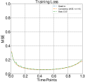
Figure 6: Expectation of training losses at different time points.

Appendix F Cost-of-Fit Analysis for Scenarios with Different $t$

The optimization objective of DPMs is very different from the usual deep learning optimization objective, and one of the key differences is that DPMs has an additional input: the time point $t$. Ideally, the velocity estimation models corresponding to the different time points can form a set of functions: $\{f_{\theta}(\cdot,t)\}_{t}$. The number of neural network parameters is so large that most studies today apply weight sharing for velocity estimation models at different time steps, thus reducing storage costs. This approach also poses a problem at another level, in that at the end of the training phase, the expectation of training losses of the velocity estimation model at different time points varies considerably, as illustrated in Fig. 6. Specifically, the expectation of the training loss will be greater as $t\rightarrow\epsilon$ or $t\rightarrow 1$, and smaller as $t\rightarrow 0.5$. This result is in line with our expectations, because as $t\rightarrow\epsilon$, the input is essentially free of Gaussian noise and can be approximated as $X_{0}$, but the output has to be predicted as $X_{1}-X_{0}$, when $X_{1}$ is completely unknowable and therefore extremely difficult. Similarly, as $t\rightarrow 1$, the input is essentially Gaussian noise and can be approximated as $X_{1}$, but the output has to be predicted as $X_{1}-X_{0}$, when $X_{0}$ is completely unknowable and therefore also equally difficult.

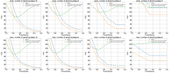
Figure 7: The figure demonstrates that replacing continuous time steps with discrete time steps to perform CUD is not a feasible approach. The discrete time step is represented by $t$ ranging from $\frac{1}{N}$ to $\frac{N}{N}$, where $N$ is set to 16 by default. On the other hand, the continuous time step is represented by $t$ ranging from $\epsilon$ to 1.

Appendix G Final Multi-Step Distillation

Table 4: Ablation experiments on final multi-step distillation. One-step: vanilla one-step distillation technique introduced in [25]. Multi-step: Our proposed final multi-step distillation without SAM. Multi-step+SAM: Our proposed final multi-step distillation with SAM.

Dataset	Metric	One-step	Multi-step	Multi-step+SAM
CIFAR-10	FID($\downarrow$)	5.78	3.74	3.77
	IS($\uparrow$)	9.43	9.21	10.45
MNIST	FID($\downarrow$)	8.94	4.80	6.38
	IS($\uparrow$)	2.08	2.10	2.12

Table 5: Verification of FID and IS at the end of each distillation step in final multi-step distillation. FID: FID is evaluated at the end of the current step. IS: IS is evaluated at the end of the current step. Original FID: The FID of the synthetic images at a specific step, is acquired through pre-training the model. And the synthetic images serve as the ground truth label, which needs to be aligned by final multi-step distillation.

Dataset	Step	FID($\downarrow$)	Original FID($\downarrow$)	IS($\uparrow$)
CIFAR-10	8	24.84	23.12	8.61
	11	14.36	9.72	9.25
	14	3.37	2.91	9.42
MNIST	8	12.59	13.71	2.03
	11	7.56	4.67	2.04
	14	6.38	2.80	2.08

Although CUD can accelerate sampling within a single training session, its reliance on continuous time steps necessitates fitting more time points than discrete time steps to complete the training, resulting in inferior performance compared to CD. In our experiments, merely replacing continuous time steps with discrete ones causes the model to collapse, as illustrated in Fig. 7. Thus, we adopt the distillation technique (a.k.a., one-step distillation) from [25] to fit the velocity estimation model under a single time point, enabling the model to outperform CD in a one-step sampling scenario. Importantly, we incorporate ideas from the teacher-assistant concept to enhance the original distillation technique [30]. Viewing the sample obtained in the last sampling step as a strong teacher output, the penultimate and penultimate third steps can be considered outputs from slightly weaker teachers. We can allow the model to gradually transition from an alignment time step from $1$ to $0$, effectively preventing performance degradation due to the gap between the strong teacher and the weak student.

For instance, if we have sampled 16 steps using Euler’s method, we obtain a set of “clean” images for each sampling time point. We can first distill the model based on the “clean” images obtained in step 8, followed by those from steps 11 and 14. To ensure the model acquires a flat loss landscape after training, we align the training model’s output with the EMA model’s output, an approach interpretable as Sharpness-Aware Minimization (SAM) [6]. In final multi-step distillation, aligning the outputs of the training model and the EMA model does not always yield successful results. Thereby, we regard this approach as an optional method.

In our experiments, we employ final multi-step distillation using “clean” images obtained at steps 8, 11, and 14 with a sampling of 16 steps through Euler’s method. To confirm the enhanced efficiency of our method compared to one-step distillation, we conduct comparative experiments and present the results in Table 4. Final multi-step distillation demonstrates a significant improvement in FID evaluation compared to one-step distillation, indicating the effectiveness and reasonableness of the multi-stage guided distillation. The positive impact of SAM is less evident and only boosts IS without affecting FID. Furthermore, the effectiveness of each step in final multi-step distillation is illustrated in Table 5. By guiding the training model through distillation using “clean” images from different steps, the synthetic images produced by the training model progressively improve in quality.

Appendix H Discussion

Limitation.

The CUD algorithm, which requires no pre-trained weights and a single training session, has considerably enhanced sampling acceleration compared to traditional DPM training paradigms. However, when assessed on the FID, a discernible performance gap with two-stage distillation-based accelerated sampling algorithms persists. This shortfall arises from two main factors: (1) Unlike those two-stage counterparts, which are trained on discrete time steps and necessitate a minimal number of time points to be fitted, CUD optimizes the loss function based on continuous time steps, demanding an infinite number of time points to be fitted. Yet, applying CUD directly to discrete time steps, as illustrated in Fig. 7, leads to training collapse due to instability. (2) CUD’s training duration is significantly shorter than that of two-stage distillation-based accelerated sampling algorithms.

Addressing this issue is a future work. This will involve revisiting hyperparameter selection and incorporating regularization terms to enhance training stability, thus enabling CUD to maintain stability over discrete time steps.

Broader Impact.

The idea of CUD is straightforward. It posits that the velocity estimation model output should align with the output from the same model at the previous moment, while simultaneously maintaining alignment with the ground truth label. This principle is anticipated to find broad application in future DPM training, potentially emerging as a more generalized paradigm. Consequently, we posit that CUD will exert a predominantly positive, rather than negative, impact on the community.

Appendix I Additional Experimental Results

In this section, we present a series of experimental results that can not fit in the main paper due to space constraints, including Tables 6,  7, 9, 9, 10, and Fig. 8. Tables 6 and 7 supplement the ablation experiments for Basic CUD in the main paper, while Tables 9, 9, and 10 supplement the comparison experimental results in the main paper. In particular, Tables 9, 9 are evaluated over samples sampled by the classical solver, including Euler and Heun, and Table 10 is evaluated over samples sampled by training-free accelerated sampling solvers, including DPM-solver-2 and Deis-2 [45].

We investigate the necessity of ground truth label supervision in this paragraph, showcasing both the Runge-Kutta-based multi-step alignment distillation that incorporates ground truth label supervision and its counterpart without such supervision in Fig. 8. The label “Runge-Kutta 23 (w/o GT)” signifies CUD lacking the loss term $\textrm{MSE}(\widetilde{X}1-X_{0},g_{\psi 2}(f_{\theta}(X_{t},t)))$, while “Runge-Kutta 23 (with GT)” denotes the same algorithm but includes this loss term. Similarly, “Runge-Kutta 34 (w/o GT)” indicates CUD without the loss terms $\textrm{MSE}(\widetilde{X}_{1}-X_{0},g{\psi 2}(f_{\theta}(X_{t},t)))$ and $\textrm{MSE}(\widetilde{X}1-X_{0},g{\psi 3}(f_{\theta}(X_{t},t)))$, and “Runge-Kutta 23 (with GT)” implies the inclusion of these loss terms. The ground truth supervision is essential for CUD, as it helps circumvent improper gradient updates that could arise from unsupervised distillation and thus adversely affect performance. As a result, for $\mathcal{L}_{\textrm{base}}$ in the main paper, we incorporate ground truth supervision into each head of the velocity estimation model $f\textemdash\textemdash\theta(\cdot,\cdot)$.

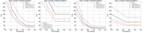
Figure 8: Ablation experiments on Runge-Kutta-based multi-step alignment distillation.

Table 6: Extension of Table 1. Additional experimental results on IS metric.

Methods		RF (Eq. 2)	Consistency Model (CD)			Basic CUD
Settings		MSE	MSE, $h\rightarrow 0$	MSE, $h\!=\!1/16$	LPIPS,$h\!=\!1/16$	MSE,$h\!=\!1/16$,	LPIPS,$h\!=\!1/16$,	MSE,$h\!=\!1/16$,	LPIPS,$h\!=\!1/16$,
						vanilla weight	vanilla weight	dynamic weight	dynamic weight
IS	Euler, 4	7.07	7.43	1.32	1.18	9.22	1.18	4.41	1.19
	Euler, 16	8.85	9.19	1.33	1.19	10.20	1.18	3.98	1.18
	Heun, 4	8.50	8.73	1.33	1.19	9.52	1.18	3.76	1.18
	Heun, 16	9.16	9.43	1.33	1.19	9.94	1.18	3.87	1.18

Table 7: Extension of Table 1. Additional experimental results on the loss function “ML”. “ML” denotes “MSE+LPIPS”, i.e., $\omega_{1}(i)\textrm{LPIPS}(\widetilde{X}_{t-h},f_{\theta}(X_{t},t))+\omega_{2}(i)\textrm{MSE}(\widetilde{X}_{1}-X_{0},f_{\theta}(X_{t},t))$.

Methods		RF (Eq. 2)	Basic CUD
Settings		MSE	ML,$h\!=\!1/16$,	ML,$h\!=\!1/16$,
			vanilla weight	dynamic weight
FID	Euler, 4	37.05	171.56	302.70
	Euler, 16	6.85	129.83	275.02
	Heun, 4	13.58	130.10	270.85
	Heun, 16	4.15	128.48	340.82
IS	Euler, 4	7.07	3.45	1.75
	Euler, 16	8.85	3.54	1.86
	Heun, 4	8.50	3.54	1.91
	Heun, 16	9.16	3.55	1.69

Table 8: Additional experimental results leveraging Euler and Heun on CIFAR-10.

    METHOD Solver NFE ($\downarrow$) FID ($\downarrow$) IS ($\uparrow$) Diffusion Model (One Stage)   Curvature [23] Euler 16 6.85 8.84 Curvature Euler 4 37.05 7.07 Curvature Heun 7 13.58 8.49 Curvature Heun 31 4.15 9.16 CUD (Runge-Kutta 12) Euler 15 2.91 9.90 CUD (Runge-Kutta 12) Euler 4 17.40 9.38 CUD (Runge-Kutta 12) Heun 7 5.38 9.61 CUD (Runge-Kutta 12) Heun 31 3.24 9.75 CUD (Runge-Kutta 23) Euler 15 3.06 9.36 CUD (Runge-Kutta 23) Euler 4 12.23 8.39 CUD (Runge-Kutta 23) Heun 7 5.07 9.20 CUD (Runge-Kutta 23) Heun 29 4.49 9.45 CUD (Runge-Kutta 34) Euler 14 3.40 9.39 CUD (Runge-Kutta 34) Euler 4 9.45 8.50 CUD (Runge-Kutta 34) Heun 7 4.70 9.34 CUD (Runge-Kutta 34) Heun 25 4.38 9.66 2-Rectified flow^∗ Euler 1 4.85 9.01  

Table 9: Additional experimental results leveraging Euler and Heun on MNIST.

    METHOD Solver NFE ($\downarrow$) FID ($\downarrow$) IS ($\uparrow$) MNIST (One Stage)   Curvature [23] Euler 16 21.77 2.11 Curvature Euler 4 49.96 2.02 Curvature Heun 7 21.55 2.10 Curvature Heun 31 18.56 2.12 CUD (Runge-Kutta 12) Euler 16 3.39 2.01 CUD (Runge-Kutta 12) Euler 4 9.45 2.02 CUD (Runge-Kutta 12) Heun 31 3.49 2.12 CUD (Runge-Kutta 12) Heun 7 3.06 2.05 CUD (Runge-Kutta 23) Euler 16 2.18 2.10 CUD (Runge-Kutta 23) Euler 4 7.06 2.03 CUD (Runge-Kutta 23) Heun 31 2.37 2.12 CUD (Runge-Kutta 23) Heun 7 2.81 2.05 CUD (Runge-Kutta 34) Euler 16 1.81 2.10 CUD (Runge-Kutta 34) Euler 4 6.70 2.03 CUD (Runge-Kutta 34) Heun 31 1.87 2.12 CUD (Runge-Kutta 34) Heun 7 2.87 2.05 PD Euler 1 13.64 2.18  

Table 10: Additional experimental results leveraging DPM-solver-2 and Deis-2 on CIFAR-10.

METHOD	Solver
	DPM-solver-2 (NFE=7)		DPM-solver-2 (NFE=4)		Deis-2 (NFE=7)		Deis-2 (NFE=4)
	FID ($\downarrow$)	IS ($\uparrow$)	FID ($\downarrow$)	IS ($\uparrow$)	FID ($\downarrow$)	IS ($\uparrow$)	FID ($\downarrow$)	IS ($\uparrow$)
CUD (Runge-Kutta 12)	3.27	9.54	8.25	8.95	4.70	9.76	8.53	9.15
CUD (Runge-Kutta 23)	3.53	9.35	6.42	8.90	4.90	9.43	6.30	8.99
CUD (Runge-Kutta 34)	4.55	9.33	6.97	8.95	6.30	8.99	5.35	9.35

Appendix J Implementation Details

Table. 11 shows the training and architecture configuration we use in our experiments. For CIFAR-10, MNIST, and ImageNet-64 datasets, we carry out three different configurations (i.e., (a), (b), and (c)) for experiments, where configurations (a) and (b) are following [23] and the model architecture in configuration (c) is following [40]. We ran the code on NVIDIA Tesla A100 GPUs, where configurations (a) used 4 GPUs with a batch size of 32 on each GPU. Configuration (b) applied 4 GPUs with a batch size of 64 on each GPU. Configuration (c) applied 8 GPUs with a batch size of 128 on each GPU. Configuration (d) is used for the final multi-step distillation, and its batch size and the learning rate are strongly correlated with the dataset. For example, if the final discrete distillation is performed on MNIST, then its batch size and learning rate are the same as configuration (b).

Table 11: Architecture and training configurations on CIFAR-10, MNIST and ImageNet-64.

	CIFAR-10 (a)	MNIST (b)	ImageNet-64 (c)	Final Multi-Step Distillation (d)
Iterations	500k	50k	500k	40k$\times$3
Batch size	128	256	1024	128/256/-
Learning rate	2e-4	3e-4	2e-4	2e-4/3e-4/-
LR warm-up steps	5000	8000	0	0
EMA decay rate	0.9999	0.9999	0.9999	0.9999
EMA start steps	1	300	1	1
Dropout probability	0	0.13	0.0	0.0
Channel multiplier	128	32	192	-
Channels per resolution	$[2,2,2]$	$[2,2,2]$	$[1,2,3,4]$	-
Xflip augmentation	0	X	X	X
# of params (generator)	55.73M	2.2M	295.90M	-
# of params (encoder)	2.2M	2.2M	-	-
# of ResBlocks	4	2	3	-
$t$ range	$[1e-5,1]$	$[1e-5,1]$	$[1e-5,1]$	-

Appendix K Additional Content Presentation

When $t\rightarrow\epsilon$, the comparison between the curves in Figs. 4 and 5 in the main paper are not fuzzy. Therefore, we present the specific data in Table 12 and 13. These tables are labeled in exactly the same form and with the same data content as Figs. 4 and 5.

Table 12: Ablation experiments on whether to use the EMA model for CUD.

Method	$\hat{h}$	N	ODE Solver	Time Points
				$\frac{16}{16}$	$\frac{15}{16}$	$\frac{14}{16}$	$\frac{13}{16}$	$\frac{12}{16}$	$\frac{11}{16}$	$\frac{10}{16}$	$\frac{9}{16}$	$\frac{8}{16}$	$\frac{7}{16}$	$\frac{6}{16}$	$\frac{5}{16}$	$\frac{4}{16}$	$\frac{3}{16}$	$\frac{2}{16}$	$\frac{1}{16}$
Baseline	$\frac{1}{16}$	16	Euler	292.58	225.57	178.35	135.57	100.76	75.11	56.83	43.61	33.97	26.83	21.34	17.15	13.68	10.86	8.59	6.85
		8	Euler	292.58		188.48		116.05		69.85		43.18		27.91		18.83		13.58
		4	Euler	292.58				145.44				69.17				37.05
		2	Euler	292.58								123.29
		16	Heun	245.83	191.65	142.16	102.29	73.65	54.48	41.33	32.01	25.24	20.15	16.12	12.74	9.84	7.28	4.84	4.16
		8	Heun	214.08		123.26		66.11		37.31		22.47		13.79		7.83		6.29
		4	Heun	170.07				57.80				19.32				13.58
		2	Heun	123.29								65.18
Runge-Kutta 12 ($f_{\theta_{-}}$)	$\frac{1}{16}$	16	Euler	138.92	101.45	73.48	55.80	44.54	36.79	31.10	26.49	22.82	18.72	15.39	12.67	10.58	7.88	8.94	13.46
		8	Euler	138.92		75.92		45.84		30.39		20.81		13.54		8.84		7.56
		4	Euler	138.92				51.72				21.08				7.92
		2	Euler	138.92								34.27
		16	Heun	114.15	80.80	60.33	48.32	40.59	34.97	30.44	26.43	22.69	19.21	16.20	13.73	10.60	10.19	14.85	17.65
		8	Heun	91.24		51.83		35.36		25.81		18.31		12.66		9.15		10.76
		4	Heun	63.26				23.82				9.13				7.57
		2	Heun	34.28								15.75
Runge-Kutta 12 ($f_{\theta}$)	$\frac{1}{16}$	16	Euler	170.70	128.28	93.18	67.27	49.31	37.09	28.58	22.20	16.89	12.34	8.58	5.84	4.25	4.09	7.19	11.08
		8	Euler	170.70		99.65		54.42		30.70		17.21		8.10		3.65		6.96
		4	Euler	63.26				23.82				9.13				7.57
		2	Euler	170.70								45.21
		16	Heun	143.21	101.73	72.04	52.49	39.80	31.40	25.27	20.23	15.81	11.97	8.93	6.89	5.68	7.78	12.65	14.79
		8	Heun	117.71		60.90		33.92		20.45		11.52		6.10		6.77		10.16
		4	Heun	81.76				22.56				4.30				4.19
		2	Heun	45.21								17.70
Runge-Kutta 23 ($f_{\theta_{-}}$)	$\frac{1}{16}$	16	Euler	102.27	77.05	59.48	46.99	38.70	33.07	29.02	25.91	23.37	21.24	19.55	18.41	17.67	16.88	16.18	15.96
		8	Euler	102.27		61.37		38.46		26.84		20.44		16.46		14.60		13.11
		4	Euler	102.27				41.06				17.90				11.31
		2	Euler	102.27								23.25
		16	Heun	85.37	64.52	51.04	42.63	37.21	33.37	30.39	27.91	25.73	23.92	22.63	21.84	21.33	20.77	20.45	20.38
		8	Heun	70.85		44.12		32.48		26.29		22.23		20.10		19.07		18.99
		4	Heun	49.40				21.68				15.12				15.75
		2	Heun	23.25								13.14
Runge-Kutta 23 ($f_{\theta}$)	$\frac{1}{16}$	16	Euler	139.64	103.35	74.87	54.49	41.09	32.14	26.10	21.72	18.37	15.77	13.69	12.15	11.35	10.74	10.11	9.71
		8	Euler	139.64		79.21		41.22		25.47		16.29		10.98		8.35		7.07
		4	Euler	139.64				50.69				16.67				6.70
		2	Euler	139.63								20.01
		16	Heun	115.70	82.15	59.34	44.95	36.05	30.21	26.13	23.04	20.58	18.59	17.05	16.16	15.64	15.10	14.61	14.50
		8	Heun	93.76		49.67		30.53		21.84		16.90		14.39		13.38		13.35
		4	Heun	62.75				19.49				9.75				10.32
		2	Heun	29.01								12.88

Table 13: Ablation experiments on whether to use the no-fix-step size and dynamic skip connection for CUD.

Method	$\hat{h}$	N	ODE Solver	Time Points
				$\frac{16}{16}$	$\frac{15}{16}$	$\frac{14}{16}$	$\frac{13}{16}$	$\frac{12}{16}$	$\frac{11}{16}$	$\frac{10}{16}$	$\frac{9}{16}$	$\frac{8}{16}$	$\frac{7}{16}$	$\frac{6}{16}$	$\frac{5}{16}$	$\frac{4}{16}$	$\frac{3}{16}$	$\frac{2}{16}$	$\frac{1}{16}$
Runge-Kutta 12 , uniform	$\frac{1}{16}$	16	Euler	235.29	179.87	133.11	96.53	70.32	52.03	38.97	29.51	23.49	17.13	12.87	9.32	6.31	3.95	3.46	4.79
		8	Euler	235.29		142.47		80.62		45.88		26.44		15.45		7.99		5.05
		4	Euler	235.29				102.27				40.94				17.64
		2	Euler	235.29								81.18
		16	Heun	199.64	145.16	102.18	72.36	52.90	39.72	30.51	23.73	18.54	14.39	10.84	7.72	5.00	3.36	4.89	6.29
		8	Heun	167.76		87.53		46.16		26.00		14.97		7.70		3.17		3.60
		4	Heun	124.11				35.99				8.56				5.40
		2	Heun	81.18								36.30
Runge-Kutta 12 , rule	$\frac{1}{16}$	16	Euler	361.05	278.28	173.90	100.28	63.26	46.67	37.97	30.96	23.84	17.60	13.30	10.66	8.92	7.52	6.64	9.19
		8	Euler	361.05		186.91		71.69		43.19		27.07		14.99		10.54		8.75
		4	Euler	361.05				90.06				38.92				18.95
		2	Euler	361.05								74.18
		16	Heun	319.92	209.83	117.32	68.82	47.83	38.14	31.80	25.69	19.73	15.07	11.96	9.86	8.18	6.79	8.11	9.16
		8	Heun	260.24		88.28		42.62		28.05		17.58		9.77		6.89		6.34
		4	Heun	146.51				36.49				10.63				8.45
		2	Heun	74.18								33.25
Runge-Kutta 23 , uniform	$\frac{1}{16}$	16	Euler	228.30	166.15	117.39	82.49	58.95	43.19	32.57	26.16	19.80	15.71	12.38	9.58	7.19	5.25	3.93	3.27
		8	Euler	228.30		126.41		67.54		37.53		21.98		13.04		7.34		4.24
		4	Euler	228.30				87.30				32.45				13.13
		2	Euler	228.30								67.08
		16	Heun	187.60	129.34	87.81	61.15	44.52	33.93	26.83	21.83	18.02	14.90	12.61	9.70	7.55	5.89	4.93	4.80
		8	Heun	151.39		73.93		38.51		22.90		14.67		9.13		5.29		4.74
		4	Heun	107.19				29.19				8.24				5.99
		2	Heun	67.08								29.03
Runge-Kutta 23 , rule	$\frac{1}{16}$	16	Euler	233.71	159.26	108.23	74.60	53.46	39.97	30.86	24.31	19.54	16.02	13.32	11.05	8.92	6.74	4.74	4.11
		8	Euler	233.71		115.43		59.76		34.30		20.84		13.49		8.64		4.74
		4	Euler	233.71				74.01				28.54				12.61
		2	Euler	233.71								56.06
		16	Heun	186.61	122.01	80.84	56.27	41.71	32.66	26.46	21.93	18.53	15.90	13.71	11.65	9.44	7.03	5.73	5.90
		8	Heun	146.03		66.79		36.25		22.78		15.63		11.00		6.40		5.56
		4	Heun	94.17				24.04				9.43				7.55
		2	Heun	56.06								24.83
Runge-Kutta 12 , uniform, $c_{\textrm{skip}}=0.25$	$\frac{1}{16}$	16	Euler	235.34	181.63	135.87	90.32	72.89	54.22	41.00	31.29	24.26	18.74	14.34	10.64	7.37	4.62	3.19	4.44
		8	Euler 235.34		145.96		83.65		48.05		28.43		16.80		9.16		5.08
		4	Euler	235.34				105.99				43.40				18.92
		2	Euler	235.34								84.16
		16	Heun	200.50	147.38	104.67	74.76	54.88	41.53	32.18	25.31	20.03	15.76	12.11	8.84	5.86	3.73	4.77	6.17
		8	Heun	170.74		99.47		48.28		27.73		16.42		8.79		3.44		3.69
		4	Heun	128.56				38.07				9.62				6.22
		2	Heun	84.16								38.55
Runge-Kutta 12 , uniform, $c_{\textrm{skip}}=0.75$	$\frac{1}{16}$	16	Euler	237.09	180.73	134.04	97.13	70.98	52.86	39.80	30.26	23.12	17.70	13.39	9.72	6.56	4.04	2.91	4.33
		8	Euler	237.09		143.74[		81.21		46.42		26.91		15.60		8.18		4.74
		4	Euler	237.09				103.04				41.26				17.40
		2	Euler	237.09								87.53
		16	Heun	199.64	145.87	102.9	73.21	53.87	40.76	31.38	24.42	19.11	14.83	11.09	7.91	5.06	3.24	4.54	5.83
		8	Heun	167.64		88.37		47.04		26.75		15.46		7.94		3.08		3.29
		4	Heun	134.37				36.49				8.75				5.38
		2	Heun	81.53								37.29

Appendix L Additional Samples from Catch-Up Distillation and Final Multi-Step Distillation

We provide additional samples from Catch-Up Distillation (CUD) and Final Multi-Step Distillation (FMSD) on MNIST (Figs. 9), CIFAR-10 (Figs. 10), and ImageNet-64 (Figs. 11).

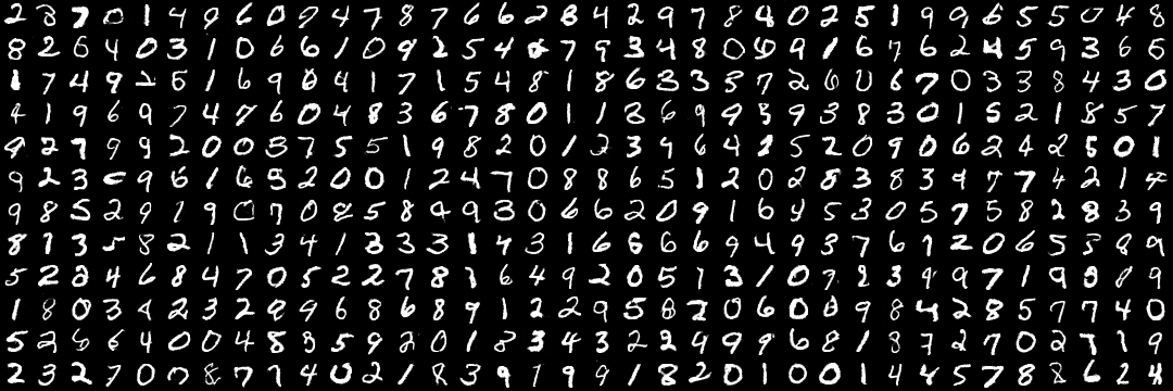
(a) FMSD with 1 step (FID=6.36)

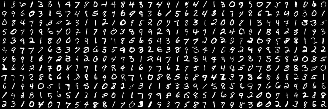
(b) CUD Runge-Kutta 12 with 16 steps (FID=3.99)

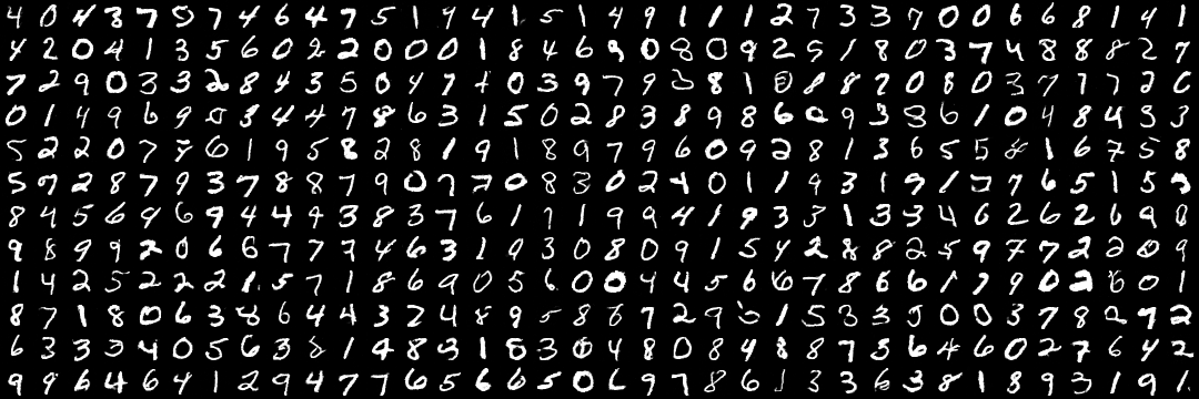
(c) CUD Runge-Kutta 23 with 16 steps (FID=2.08)

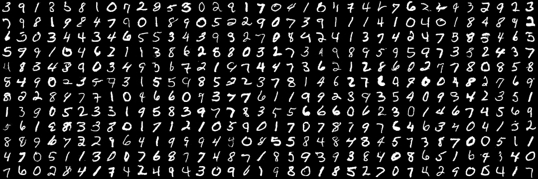
(d) CUD Runge-Kutta 34 with 16 steps (FID=1.81)

Figure 9: Synthetic images sampled from MNIST $28\times 28$.

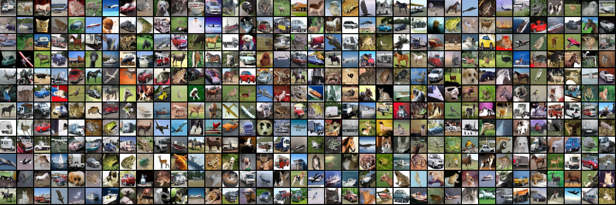
(a) FMSD with 1 step (FID=3.77)

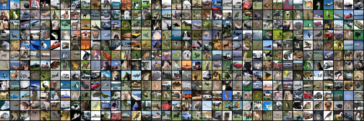
(b) CUD Runge-Kutta 12 with 15 steps (FID=2.91)

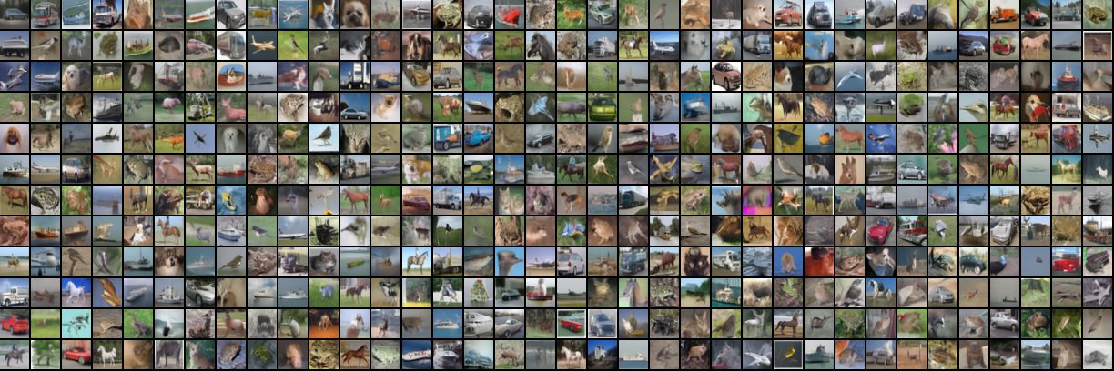
(c) CUD Runge-Kutta 23 with 4 steps (FID=12.23)

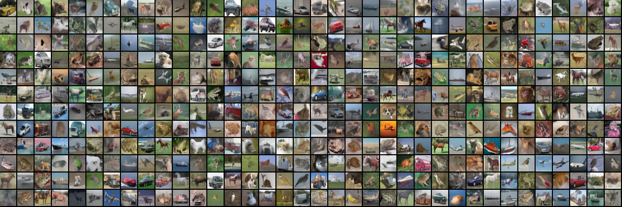
(d) CUD Runge-Kutta 34 with 4 steps (FID=9.45)

Figure 10: Synthetic images sampled from CIFAR-10 $32\times 32$.

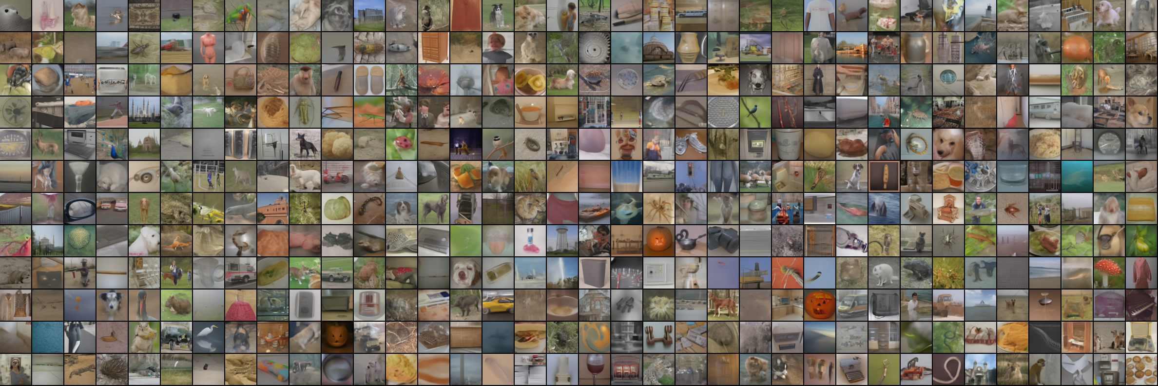
(a) CUD Runge-Kutta 12 with 4 steps (Euler, FID=18.84)

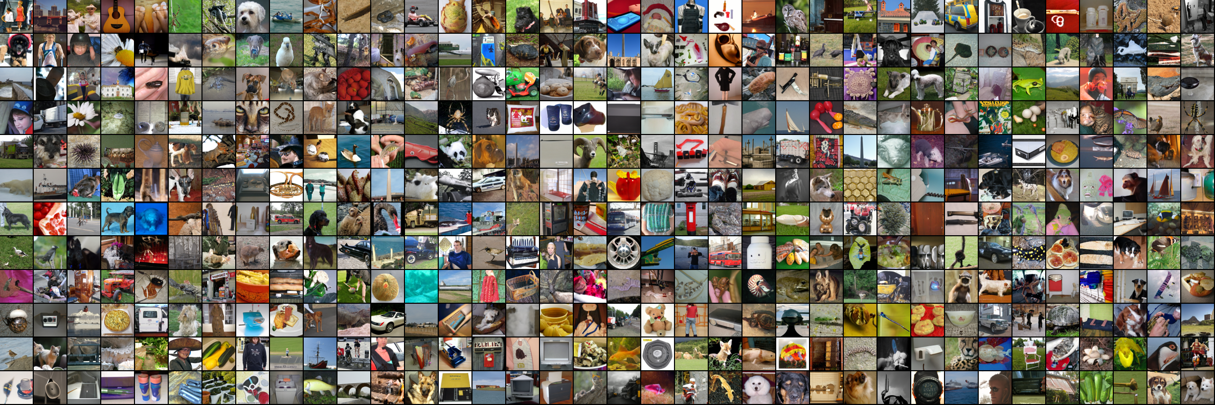
(b) CUD Runge-Kutta 12 with 16 steps (Euler, FID=5.05)

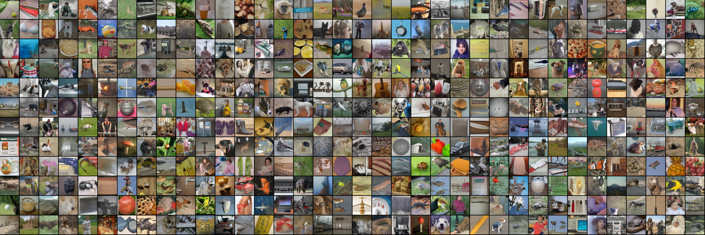
(c) CUD Runge-Kutta 12 with 8 steps (Euler, FID=7.75)

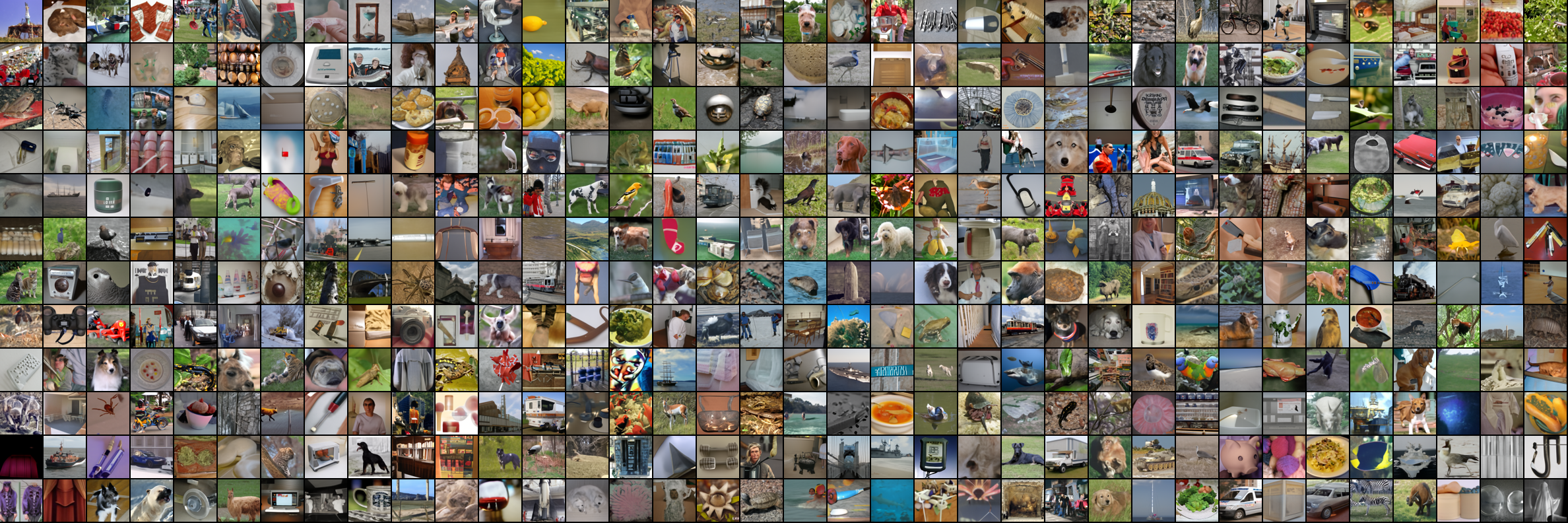
(d) CUD Runge-Kutta 12 with 6 steps (DPM-Solver-2, FID=7.68)

Figure 11: Synthetic images sampled from ImageNet-1k $64\times 64$.

References

- Bao et al. [2022] F. Bao, C. Li, J. Zhu, and B. Zhang. Analytic-dpm: an analytic estimate of the optimal reverse variance in diffusion probabilistic models. In International Conference on Learning Representations, Virtual Event, Apr. 2022. OpenReview.net.
- Brock et al. [2019] A. Brock, J. Donahue, and K. Simonyan. Large scale gan training for high fidelity natural image synthesis. In International Conference on Learning Representations, New Orleans, LA, USA, May 2019. OpenReview.net.
- Chuanguang et al. [2021] Y. Chuanguang, A. Zhulin, C. Linhang, and X. Yongjun. Hierarchical self-supervised augmented knowledge distillation. In Proceedings of the Thirtieth International Joint Conference on Artificial Intelligence, pages 1217–1223, Virtual Event, Aug. 2021. IJCAI.
- Dhariwal and Nichol [2021] P. Dhariwal and A. Q. Nichol. Diffusion models beat GANs on image synthesis. In Neural Information Processing Systems, volume 34, pages 8780–8794, Virtual Event, Dec. 2021. NIPS. URL https://openreview.net/forum?id=AAWuCvzaVt.
- Dosovitskiy et al. [2020] A. Dosovitskiy, L. Beyer, A. Kolesnikov, D. Weissenborn, X. Zhai, T. Unterthiner, M. Dehghani, M. Minderer, G. Heigold, S. Gelly, et al. An image is worth 16x16 words: Transformers for image recognition at scale. In International Conference on Learning Representations, Event Virtual, May 2020. OpenReview.net.
- Du et al. [2022] J. Du, D. Zhou, J. Feng, V. Tan, and J. T. Zhou. Sharpness-aware training for free. In Advances in Neural Information Processing Systems, volume 35, pages 23439–23451, New Orleans, Louisiana, USA, Dec. 2022. NIPS.
- Gong et al. [2019] X. Gong, S. Chang, Y. Jiang, and Z. Wang. Autogan: Neural architecture search for generative adversarial networks. In International Conference on Computer Vision, pages 3224–3234, Seoul, South Korea, Oct.-Nov. 2019. IEEE.
- Goodfellow et al. [2014] I. Goodfellow, J. Pouget-Abadie, M. Mirza, B. Xu, D. Warde-Farley, S. Ozair, A. Courville, and Y. Bengio. Generative adversarial nets. In Neural Information Processing Systems, volume 27, Long Beach, CA, USA, Jan. 2014. NIPS.
- Gou et al. [2021] J. Gou, B. Yu, S. J. Maybank, and D. Tao. Knowledge distillation: A survey. International Journal of Computer Vision, 129(6):1789–1819, 2021.
- He et al. [2016a] K. He, X. Zhang, and S. Ren. Deep residual learning for image recognition. In Computer Vision and Pattern Recognition, pages 770–778, Las Vegas, NV, USA, Jun. 2016a. IEEE.
- He et al. [2016b] K. He, X. Zhang, S. Ren, and J. Sun. Identity mappings in deep residual networks. In European Conference on Computer Vision, pages 630–645, Amsterdam, North Holland, The Netherlands, Oct. 2016b. Springer.
- Heusel et al. [2017] M. Heusel, H. Ramsauer, T. Unterthiner, B. Nessler, and S. Hochreiter. Gans trained by a two time-scale update rule converge to a local nash equilibrium. In Neural Information Processing Systems, volume 30, Long Beach Convention Center, Long Beach, Dec. 2017. NIPS.
- Hinton et al. [2015] G. Hinton, O. Vinyals, and J. Dean. Distilling the knowledge in a neural network, 2015. URL https://arxiv.org/abs/1503.02531.
- Ho and Salimans [2021] J. Ho and T. Salimans. Classifier-free diffusion guidance. In Neural Information Processing Systems Workshop, Virtual Event, Dec. 2021. NIPS. URL https://openreview.net/forum?id=qw8AKxfYbI.
- Ho et al. [2020] J. Ho, A. Jain, and P. Abbeel. Denoising diffusion probabilistic models. In Neural Information Processing Systems, pages 6840–6851, Virtual Event, Dec. 2020. NIPS.
- Karras et al. [2019] T. Karras, S. Laine, and T. Aila. A style-based generator architecture for generative adversarial networks. In Computer Vision and Pattern Recognition, pages 4401–4410, Seoul, South Korea, Oct.-Nov. 2019.
- Karras et al. [2022] T. Karras, M. Aittala, T. Aila, and S. Laine. Elucidating the design space of diffusion-based generative models. arXiv preprint arXiv:2206.00364, 2022.
- Kawar et al. [2021] B. Kawar, G. Vaksman, and M. Elad. Snips: Solving noisy inverse problems stochastically. In Neural Information Processing Systems, volume 34, pages 21757–21769, Virtual Event, Dec. 2021. NIPS.
- Kingma et al. [2021] D. Kingma, T. Salimans, B. Poole, and J. Ho. Variational diffusion models. In Neural Information Processing Systems, volume 34, pages 21696–21707, Virtual Event, 2021. NIPS.
- Kingma and Welling [2013] D. P. Kingma and M. Welling. Auto-encoding variational bayes. arXiv preprint arXiv:1312.6114, 2013.
- Kong et al. [2021] Z. Kong, W. Ping, J. Huang, K. Zhao, and B. Catanzaro. Diffwave: A versatile diffusion model for audio synthesis. In International Conference on Learning Representations, Virtual Event, May 2021. OpenReview.net. URL https://openreview.net/forum?id=a-xFK8Ymz5J.
- Krizhevsky et al. [2009] A. Krizhevsky, G. Hinton, et al. Learning multiple layers of features from tiny images. 2009.
- Lee et al. [2023] S. Lee, B. Kim, and J. C. Ye. Minimizing trajectory curvature of ode-based generative models. arXiv preprint arXiv:2301.12003, 2023.
- Li et al. [2022] H. Li, Y. Yang, M. Chang, S. Chen, H. Feng, Z. Xu, Q. Li, and Y. Chen. Srdiff: Single image super-resolution with diffusion probabilistic models. Neurocomputing, 479:47–59, 2022. ISSN 0925-2312. doi: https://doi.org/10.1016/j.neucom.2022.01.029.
- Liu et al. [2022] X. Liu, C. Gong, and Q. Liu. Flow straight and fast: Learning to generate and transfer data with rectified flow. arXiv preprint arXiv:2209.03003, 2022.
- Lu et al. [2022a] C. Lu, Y. Zhou, F. Bao, J. Chen, and C. Li. Dpm-solver++: Fast solver for guided sampling of diffusion probabilistic models. arXiv preprint arXiv:2211.01095, 2022a.
- Lu et al. [2022b] C. Lu, Y. Zhou, F. Bao, J. Chen, C. Li, and J. Zhu. Dpm-solver: A fast ode solver for diffusion probabilistic model sampling in around 10 steps. In Neural Information Processing Systems, New Orleans, LA, USA, Nov.-Dec. 2022b. NIPS.
- Luhman [2021] E. Luhman. Knowledge distillation in iterative generative models for improved sampling speed. arXiv preprint arXiv:2101.02388, 2021.
- Meng et al. [2022] C. Meng, R. Gao, D. P. Kingma, S. Ermon, J. Ho, and T. Salimans. On distillation of guided diffusion models. arXiv preprint arXiv:2210.03142, 2022.
- Mirzadeh et al. [2020] S. I. Mirzadeh, M. Farajtabar, A. Li, N. Levine, A. Matsukawa, and H. Ghasemzadeh. Improved knowledge distillation via teacher assistant. In Association for the Advance of Artificial Intelligence, volume 34, pages 5191–5198, New York, NY, USA, Feb. 2020. AAAI Press.
- Nichol and Dhariwal [2021] A. Q. Nichol and P. Dhariwal. Improved denoising diffusion probabilistic models. In International Conference on Machine Learning, pages 8162–8171. PMLR, 2021.
- Park et al. [2019] W. Park, D. Kim, Y. Lu, and M. Cho. Relational knowledge distillation. In Computer Vision and Pattern Recognition, Long Beach, CA, USA, June 2019. IEEE.
- Poole et al. [2023] B. Poole, A. Jain, J. T. Barron, and B. Mildenhall. Dreamfusion: Text-to-3d using 2d diffusion. In International Conference on Learning Representations, 2023. URL https://openreview.net/forum?id=FjNys5c7VyY.
- Ronneberger et al. [2015] O. Ronneberger, P. Fischer, and T. Brox. U-net: Convolutional networks for biomedical image segmentation. In Medical Image Computing and Computer-Assisted Intervention, pages 234–241, Germany, Central Europe, Oct. 2015. Springer.
- Runge [1895] C. Runge. Ueber die numerische auflösung von differentialgleichungen. pages 1432–1807, Jun. 1895.
- Salimans and Ho [2022] T. Salimans and J. Ho. Progressive distillation for fast sampling of diffusion models. In International Conference on Learning Representations, Virtual Event, Apr. 2022. OpenReview.net.
- Salimans et al. [2016] T. Salimans, I. Goodfellow, W. Zaremba, V. Cheung, A. Radford, and X. Chen. Improved techniques for training gans. In Neural Information Processing Systems, volume 29, Centre Convencions Internacional Barcelona, Barcelona SPAIN, Dec. 2016. NIPS.
- Song et al. [2023a] J. Song, C. Meng, and S. Ermon. Denoising diffusion implicit models. In International Conference on Learning Representations, kigali, rwanda, May. 2023a. OpenReview.net.
- Song and Ermon [2019] Y. Song and S. Ermon. Generative modeling by estimating gradients of the data distribution. In Neural Information Processing Systems, volume 32. NIPS, 2019. URL https://proceedings.neurips.cc/paper_files/paper/2019/file/3001ef257407d5a371a96dcd947c7d93-Paper.pdf.
- Song et al. [2023b] Y. Song, P. Dhariwal, M. Chen, and I. Sutskever. Consistency models. arXiv preprint arXiv:2303.01469, 2023b.
- Song et al. [2023c] Y. Song, J. Sohl-Dickstein, D. P. Kingma, A. Kumar, S. Ermon, and B. Poole. Score-based generative modeling through stochastic differential equations. In International Conference on Learning Representations, kigali, rwanda, May. 2023c. OpenReview.net.
- Sun et al. [2022] W. Sun, D. Chen, C. Wang, D. Ye, Y. Feng, and C. Chen. Accelerating diffusion sampling with classifier-based feature distillation. arXiv preprint arXiv:2211.12039, 2022.
- Vahdat and Kautz [2020] A. Vahdat and J. Kautz. Nvae: A deep hierarchical variational autoencoder. volume 33, pages 19667–19679, Virtual Event, Dec. 2020. NIPS.
- Yang et al. [2022] L. Yang, Z. Zhang, Y. Song, S. Hong, R. Xu, Y. Zhao, Y. Shao, W. Zhang, B. Cui, and M.-H. Yang. Diffusion models: A comprehensive survey of methods and applications. arXiv preprint arXiv:2209.00796, 2022.
- Zhang and Chen [2023] Q. Zhang and Y. Chen. Fast sampling of diffusion models with exponential integrator. In International Conference on Learning Representations. OpenReview.net, 2023. URL https://openreview.net/forum?id=Loek7hfb46P.
- Zhang et al. [2018] R. Zhang, P. Isola, A. A. Efros, E. Shechtman, and O. Wang. The unreasonable effectiveness of deep features as a perceptual metric. In Computer Vision and Pattern Recognition, Salt Lake City, Utah, USA, June 2018. IEEE.
- Zhu et al. [2017] J.-Y. Zhu, T. Park, P. Isola, and A. A. Efros. Unpaired image-to-image translation using cycle-consistent adversarial networks. In International Conference on Computer Vision, pages 2223–2232. IEEE, 2017.