Adversarial Amendment is the Only Force
Capable of Transforming an Enemy into a Friend

Abstract

Adversarial attack is commonly regarded as a huge threat to neural networks because of misleading behavior. This paper presents an opposite perspective: adversarial attacks can be harnessed to improve neural models if amended correctly. Unlike traditional adversarial defense or adversarial training schemes that aim to improve the adversarial robustness, the proposed adversarial amendment (AdvAmd) method aims to improve the original accuracy level of neural models on benign samples. We thoroughly analyze the distribution mismatch between the benign and adversarial samples. This distribution mismatch and the mutual learning mechanism with the same learning ratio applied in prior art defense strategies is the main cause leading the accuracy degradation for benign samples. The proposed AdvAmd is demonstrated to steadily heal the accuracy degradation and even leads to a certain accuracy boost of common neural models on benign classification, object detection, and segmentation tasks. The efficacy of the AdvAmd is contributed by three key components: mediate samples (to reduce the influence of distribution mismatch with a fine-grained amendment), auxiliary batch norm (to solve the mutual learning mechanism and the smoother judgment surface), and AdvAmd loss (to adjust the learning ratios according to different attack vulnerabilities) through quantitative and ablation experiments.

1 Introduction

The success of neural networks has brought a radical improvement in applications for human beings’ daily life. Meanwhile, the concerns about the robustness and safety of the neural networks also increase. Szegedy et al. (2013) proved that by maximizing the prediction error, the neural model will always classify an image to a misleading category by applying a certain hardly perceptible perturbation. What is worse, this is not a random artifact of the neural network learning process. In contrast, this is a common issue. And the perturbed inputs are termed “adversarial samples”. Since then, much attention has been put on the study of the adversarial attack, which is a technique that attempts to fool neural networks with deceptive data Goodfellow et al. (2014).

Adversarial attack is commonly regarded as a growing and massive threat to the industry and research community because of its misleading behavior toward neural networks. With the in-depth study, adversarial attacks are proved to be effective in flexibly generating adversarial examples to deceive a range of applications, especially in the computer vision field, such as classification Moosavi-Dezfooli et al. (2016), semantic segmentation Xu et al. (2020), face recognition Mirjalili and Ross (2017), and depth estimation Zhang et al. (2020), also in the natural language processing field for recognition Cisse et al. (2017), generation Liang et al. (2017), and translation Belinkov and Bisk (2017) tasks. Various adversarial defense strategies have been proposed, including modifying input data Tramèr et al. (2017) Dziugaite et al. (2016), modifying to regularize neural models Papernot et al. (2016) Lyu et al. (2015), and using auxiliary tools Meng and Chen (2017) Samangouei et al. (2018) to improve the robustness and safety of models against various adversarial attacks. Our method belongs to neither area, i.e., it first applies the adversarial attack to generate attack samples, then amends the attack samples and the adversarial defense process to achieve robustness and boost the accuracy on the original benign dataset, simultaneously.

The typical purpose of the adversarial attack is to add a natural perturbation to the benign input samples to generate the corresponding adversarial samples, which may cause a specific malfunction in the target model. Meanwhile, the adversarial perturbation is hardly perceptible, so humans can still correctly recognize the adversarial samples. The principle for most prior art adversarial attacks is changing the gradient step to a misleading direction when calculating the loss function during the back-propagation. The naive defense strategy is generating such adversarial samples and mixing them with benign samples to perform the mutual learning for neural models and make them more robust to adversarial attacks. However, such mutual learning is based on the assumption that the adversarial and benign samples have a similar distribution, which is not necessarily correct, as observed from the experiment results in Table 1. Because if the assumption stands, both the model accuracy metric on adversarial and metric on benign samples should increase. But in fact, we find such a defense strategy has a side-effect on the model capacity on benign samples, i.e., leading to noticeable accuracy degradation on the benign dataset.

Inspired by the findings that the defense against adversarial attack (details in Section 3) may lead to the accuracy degradation on benign samples, this paper focuses on solving this issue. We stand on an opposite perspective to previous studies, i.e., if the adversarial attack can be amended properly and in the right direction, the attack can be harnessed and transferred to improve the neural models’ accuracy. Besides the similarity in the workflow, the purpose of our technique is totally different from traditional adversarial defense or adversarial training methods, which aim at improving the adversarial robustness, i.e., the accuracy after introducing adversarial samples. In contrast, our proposed adversarial amendment method aims to improve the original capabilities of neural models, i.e., the accuracy induced by benign samples. Our main contributions include:

• The qualitative explanation and theoretical proof illustrate the distribution mismatch and the mutual learning mechanism cause the accuracy degradation for benign samples. (Section 3)

• AdvAmd is featured with involving mediate samples, inserting auxiliary batch norm, and applying AdvAmd loss. It solves the mismatch and tangled distribution with fine-grained data argumentation and learning adjustment according to attack vulnerabilities. (Section 4)

• We validate the efficacy of AdvAmd both on benign and adversarial samples. On several classification, detection and segmentation models, and results show that our AdvAmd method can achieve about $\textbf{1.2\%}\sim\textbf{2.5\%}$ metric increase to on benign samples without side-effect on robustness against adversarial samples. (Section 5)

2 Related Work

In our proposed method, we need to apply the adversarial attack to generate the adversarial samples, so we first go through the standard adversarial attack methods. Though adversarial defense has a different purpose from the proposed amendment, it has a similar workflow. So we also review the adversarial defense methods for further distinction.

2.1 Adversarial Attack

Based on whether or not having access to the target model, the adversarial attack methods Ozdag (2018) can be divided into the black-box and the white-box categories. Because our aim is amending the adversarial attack to boost the accuracy of the original model, the assumption is having access to the model which belongs to the white-box attack category.

White-box attack. In this category, the full knowledge of the target model, including architecture, parameters, training method and dataset, is assumed to be known. And the adversarial attacker can fully utilize the available information to analyze the most vulnerable points of the target model. Goodfellow et al. (2014) proposed the Fast Gradient Sign Method (FGSM), which calculates the gradient of the cost function during the back-propagation, then generates the adversarial examples by changing one gradient sign step. Basic Iterative Method (BIM) Kurakin et al. (2016) and Projected Gradient Descent (PGD) Madry et al. (2018) are the straightforward extension of FGSM by applying a FGSM attack multiple times with a small step size. Moosavi-Dezfooli et al. (2016) proposed a DeepFool attack to compute a minimal norm perturbation in an iterative manner to find the decision boundary and find the minimal adversarial samples across the boundary. Cisse et al. (2017) proposed a Houdini attack, which is demonstrated to be effective in generating perturbations to deceive gradient-based networks used in image classification and speech recognition tasks. In our amendment workflow, we mainly apply FGSM, PGD and DeepFool to generate the adversarial samples.

2.2 Adversarial Defense

A mass of adversarial defense methods have been proposed to improve the robustness of neural models against the adversarial attack, which can be divided into three main categories: modifying data, modifying models, and using auxiliary tools. The defense strategy in the first category does not directly deal with the target models. In contrast, the other two categories are more concerned with the target models themselves.

Data modification. Adversarial training is the most widely used method in this category. Szegedy et al. (2013) injected adversarial samples and modified their labels to improve the robustness of the target model. Huang et al. (2015) increased the robustness of the target model by punishing misclassified adversarial samples. The limitation of this strategy is that if all unknown adversarial samples are introduced into the training then the accuracy will be decreased on benign samples. In contrast, introducing some of the adversarial samples is often not enough to remove the impact of the adversarial perturbation. The mediate samples proposed in our amendment method can provide fine-grained data modification as a fix.

Model modification. The popular strategy is defensive distillation. This kind of strategy extends the knowledge distillation Hinton et al. (2015) to producing a new target model with a smoother output surface Papernot et al. (2016) Papernot and McDaniel (2017), that is less sensitive to adversarial perturbations to improve the robustness. However, the smoother output surface may also lead the model to make “new” mistakes when detecting the benign samples, which is proved in Section 3. It inspires us to apply two separate batch norms for learning from benign and adversarial samples, which can improve robustness and simultaneously keep the sharper output surface.

Auxiliary tools utilization. Researchers also came up with defense strategies by using auxiliary tools.The successful strategy is proposed as MagNet Meng and Chen (2017). MagNet uses an auxiliary detector to identify the benign and adversarial samples by measuring the distance between a given test sample and the manifold, then rejects the sample if the distance exceeds the threshold. However, based on our experiments in Table 1, it still leads the accuracy degradation on benign samples. It inspires us the necessity to adjust the learning ratios for different samples according to different attack vulnerabilities.

3 Existing Defense Strategies Lead to Accuracy Degradation On Benign Samples

The existing adversarial defense strategies are effective and helpful to target models’ adversarial robustness, i.e., boosting the target models’ accuracy when testing on adversarial samples. Some prior works find these strategies may lead to the accuracy degradation on benign samples Meng and Chen (2017) Madry et al. (2018) Xie et al. (2019) for the basic classification task. Because object detection is more complicated than classification, we want to verify whether such accuracy degradation is also valid in the object detection task. We validate by choosing the representative defense method in each category (adversarial training Szegedy et al. (2013) (Adv-Train), defensive distillation Papernot and McDaniel (2017) (Def-Distill), and MagNet Meng and Chen (2017)) and apply them to several typical object detection models, i.e., Faster R-CNN Ren et al. (2015), SSD Liu et al. (2016), RetinaNet Lin et al. (2017), YOLO Jocher (2022)) to test the corresponding accuracy on the benign and adversarial COCO dataset Lin et al. (2014). The adversarial dataset is generated by FGSM Goodfellow et al. (2014) and PGD Madry et al. (2018) attacks. More details can refer to Experiments Settings.

Network	Baseline Box AP	Defense Type	$\Delta$ Box AP on Adversarial Dataset				$\Delta$ Box AP on Benign Dataset
			FGSM Attack		PGD Attack		FGSM Attack		PGD Attack
			$\epsilon$=0.01	$\epsilon$=0.1	$\epsilon$=0.01	$\epsilon$=0.1	$\epsilon$=0.01	$\epsilon$=0.1	$\epsilon$=0.01	$\epsilon$=0.1
Faster R-CNN (RN50)	37.0	None	-5.1	-9.3	-6.5	-11.1	0.0	0.0	0.0	0.0
		Adv-Train	-2.8	-5.4	-3.8	-6.8	-1.3	-3.0	-2.0	-3.2
		Def-Distill	-2.6	-5.3	-3.8	-6.7	-1.4	-3.0	-2.0	-3.3
		MagNet	-2.2	-5.4	-3.7	-6.6	-1.7	-3.2	-2.3	-3.5
SSD (RN50)	25.8	None	-4.7	-8.7	-5.6	-9.8	0.0	0.0	0.0	0.0
		Adv-Train	-2.4	-5.4	-3.9	-6.2	-0.7	-1.8	-1.4	-2.1
		Def-Distill	-2.0	-5.1	-3.6	-6.0	-0.8	-1.9	-1.5	-2.3
		MagNet	-1.8	-4.9	-3.5	-5.9	-0.9	-2.1	-1.5	-2.4
RetinaNet (RN50)	36.4	None	-5.0	-9.1	-6.4	-10.9	0.0	0.0	0.0	0.0
		Adv-Train	-2.7	-5.3	-3.7	-6.7	-1.3	-2.9	-1.9	-3.1
		Def-Distill	-2.5	-5.2	-3.7	-6.6	-1.4	-3.0	-1.9	-3.2
		MagNet	-2.2	-5.3	-3.6	-6.5	-1.6	-2.9	-2.0	-3.4
YOLO-V5 (Large)	48.6	None	-6.9	-12.2	-8.5	-14.8	0.0	0.0	0.0	0.0
		Adv-Train	-3.8	-6.4	-4.7	-7.9	-2.2	-4.5	-3.2	-5.3
		Def-Distill	-3.6	-6.3	-4.5	-7.6	-2.4	-4.6	-3.4	-5.4
		MagNet	-3.4	-6.2	-4.4	-7.6	-2.5	-4.8	-3.5	-5.5

Table 1: Adversarial defense strategies effectiveness on detection models. ($\epsilon$: perturbation epsilon)

From the results shown in Table 1, we can draw two conclusions. The adversarial defense methods effectively improve the adversarial robustness, i.e., the accuracy of the adversarial dataset has been obviously recovered. On the other hand, the accuracy degradation on the benign dataset is also valid for the detection models. The detection models “enhanced” with defense methods obtain lower accuracy on benign datasets than their vanilla baselines. If the adversarial dataset is attacked with more strength and generated with more perturbations, the accuracy degradation will be more noticeable when passing the adversarial defense “enhancement”. Therefore, the diverse behaviors on the adversarial and benign dataset prove the assumption that the adversarial and benign samples have a similar distribution does not stand. So the mutual learning on benign and adversarial samples in the adversarial defense methods cannot avoid the accuracy degradation on the benign samples if they also want to keep the high adversarial robustness. This dilemma is the key issue to be solved in this paper.

3.1 Qualitative Explanation

We hypothesize such accuracy degradation for benign samples is mainly caused by distribution mismatch and fuzz. Though the adversarial perturbations are slight in magnitude, the distribution of the adversarial samples differs from the benign counterparts. The essential concepts of adversarial training and MagNet are both harnessing the adversarial samples with the corrected label information in the corresponding regions in the benign samples, then involving these processed samples with vanilla benign samples in adversarial training. The supervised training samples from two different sets with different distributions will make the judgment boundary fuzzy. The defensive distillation aims to produce an enhanced target model with a smoother output surface, also eventually fuzzing the boundary. With the vague boundary, the target model will make fewer mistakes when detecting the adversarial samples but may also make “new” mistakes when detecting the benign samples.

(a) Vanilla Object Detection

(b) Adversarial Attack

(c) Adversarial Defense

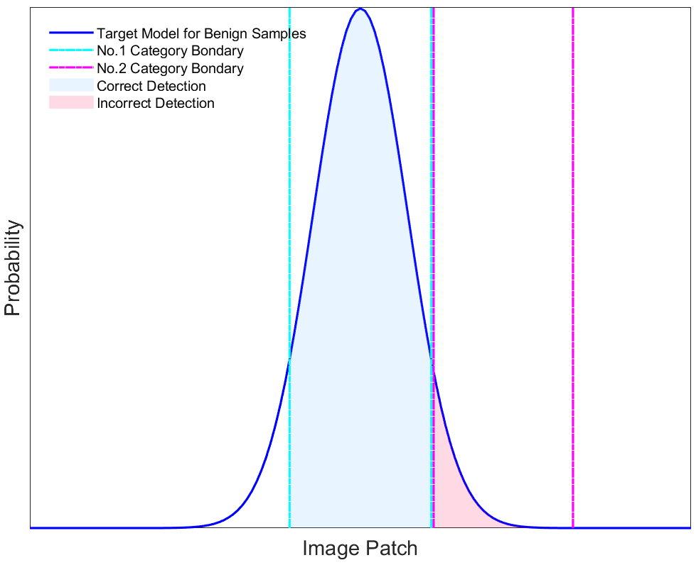
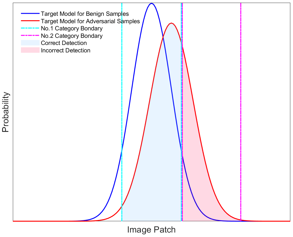
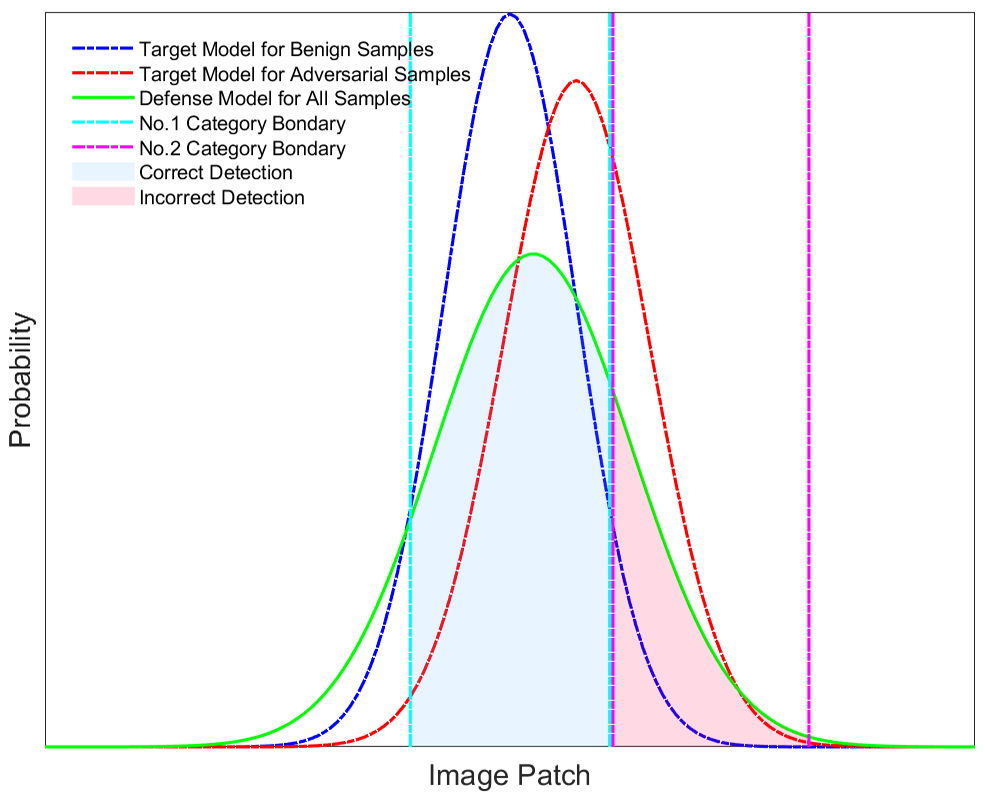
Figure 1: Qualitative explanation for adversarial attack and defense influence. Comparison between (a) and (b) helps to explain why the model is misleading by adversarial samples. Comparison between (b) and (c) helps to explain why the defense model has better adversarial robustness to the adversarial samples. Comparison between (a) and (c) helps to explain the accuracy degradation for benign samples.

We illustrate the qualitative explanation based on the hypothesis, as shown in Figure 1. To be clear, we only pay close attention to two object categories divided and marked by the boundaries in the figure. For a vanilla-trained object detection model, its judgment distribution to the benign samples is shown in Figure 1 (a). The corresponding area filled with light blue background color represents the model’s correct detection for the No.1 category. In contrast, the area filled with light red represents the incorrect detection, i.e., detecting the objects belonging to the No.1 category as the No.2 category. As shown in Figure 1 (b), when the adversarial attack perturbs the benign samples, the distribution of the adversarial samples drifts from the benign counterparts, and so do the correct and incorrect detection areas. The incorrect detection area size is obviously enlarged, which aligns with the phenomenon that the model is misleading by some adversarial samples. Then the adversarial defense method is applied, as shown in Figure 1 (c). Based on the explanation mentioned above, the label info correction in each defense strategy will not alter the model judgment distribution before the defense process. The defense training process obtains info from both benign and adversarial distribution, producing a defense model with a smoother judgment distribution. Compared to Figure 1 (b), the incorrect detection area is diminished, which aligns with the phenomenon that the defense model has better adversarial robustness to the adversarial samples. We also notice the right detection area size is smaller than the counterpart in Figure 1 (a) due to the smoother judgment surface. That helps explain why the accuracy degradation for benign samples occurs qualitatively.

3.2 Theoretical Proof

Starting from the two-category detection situation, assume the aforementioned vanilla-trained model’s judgment distributions to the benign and adversarial samples are two normal random variables $X$, $Y$ with means $\mu_{x}$, $\mu_{y}$ and variances $\sigma_{x}^{2}$, $\sigma_{y}^{2}$., which can be expressed as follows:

$$X\sim N\left(\mu_{x},\sigma_{x}^{2}\right),\quad Y\sim N\left(\mu_{y},\sigma_{y}^{2}\right)$$ (1)

Theorem: Mutual probability distribution of the linear combination of multiple normal random variables: $X_{1}\sim N\left(a_{1}\mu_{1},A_{1}^{2}{\sigma_{1}}^{2}\right)$, $X_{2}\sim N\left(a_{2}\mu_{2},A_{2}^{2}{\sigma_{2}}^{2}\right)$ $\cdots X\sim N\left(a_{n}\mu_{n},A_{n}^{2}{\sigma_{n}}^{2}\right)$ can be expressed as: $Z=\sum_{i=1}^{n}c_{i}X_{i}\sim N\left(\sum_{i=1}^{n}c_{i}a_{i}\mu_{i},\sum_{i=1}^{n}c_{i}^{2}A_{i}^{2}{\sigma_{i}}^{2}\right)$.

From the Theorem we can find the mutual probability distribution has larger variances than each variance for each individual distribution. And the larger variance value leads to the smoother judgement boundary for the defense model, which helps explain why the accuracy degradation for benign samples occurs in theory.

4 Adversarial Amendment is Capable of Transforming an Enemy into a Friend

Based on the qualitative explanation and theoretical proof, we find the distribution mismatch between the benign and adversarial samples, and the mutual learning mechanism widely applied in various adversarial defense strategies cause the accuracy degradation for benign samples. In this section, we propose the Adversarial Amendment (AdvAmd) method to harness the adversarial attack and samples properly, transforming these commonly regarded enemies into a friend, i.e., improving model accuracy on benign samples.

Given the supervised category info $\textbf{\emph{y}}_{c}$, the vanilla training and optimization process of target model (referred as $\textbf{\emph{M}}_{T}$) can be expressed as the following minimization problem:

$$\min_{\theta}\ \textbf{\emph{L}}(\textbf{\emph{y}},\textbf{\emph{y}}_{c})=\min_{\theta}\ \textbf{\emph{L}}(\textbf{\emph{F}}(\textbf{\emph{M}}_{T},\textbf{\emph{x}}),\textbf{\emph{y}}_{c})$$ (2)

where x is the benign input sample, y is the corresponding output of the neural function F, $\theta$ is the weight parameters of the target model $\textbf{\emph{M}}_{T}$, and $\textbf{\emph{L}}(\cdot)$ refers to the loss function used in vanilla training.

For the adversarial attack settings, the perturbation $\delta$ is added to the input x to constitute the adversarial samples $\textbf{\emph{x}}_{adv}$, subject to the $L_{*}$ perturbation constraint:

$$\left\|\textbf{\emph{x}}_{adv}-\textbf{\emph{x}}\right\|_{*}=\left\|\delta\right\|_{*}\leq\epsilon,\quad*\in\left\{0,1,2,\infty\right\}$$ (3)

where $\epsilon$ refers to the attack strength. The aim for the adversarial attack is to maximally deteriorate the benign samples and change the correct behavior of the target model within the perturbation constraint. If the whole benign dataset is defined as D, with $N$ categories, and each category is labeled with $\textbf{\emph{y}}_{c:k}$ and the subset with category $\textbf{\emph{y}}_{c:k}$ is denoted as $\textbf{\emph{D}}(\textbf{\emph{y}}_{c:k})$, then the adversarial attack process can be denoted with the following joint optimization problem.

$$\left\{\begin{matrix}\begin{aligned} &\mathop{\max_{\delta_{k}}}\sum\limits_{k=1}^{N}\sum\limits_{\textbf{\emph{x}}_{k}\in\textbf{\emph{D}}(\textbf{\emph{y}}_{c:k})}\textbf{\emph{L}}(\textbf{\emph{F}}(\textbf{\emph{M}}_{T},\textbf{\emph{x}}_{k}+\delta_{k}),\textbf{\emph{y}}_{c:k})\\ &\mathop{\min}\sum\limits_{k=1}^{N}\left\|\delta_{k}\right\|_{*},\quad\left\|\delta_{k}\right\|_{*}\leq\epsilon,\quad*\in\left\{0,1,2,\infty\right\}\\ \end{aligned}\end{matrix}\right.$$ (4)

Pain point 1: distribution mismatch between the benign and adversarial samples.

In the existing adversarial defense strategies, the supervised label of the adversarial sample is corrected by the corresponding region in the benign samples. However, the label correction in each defense strategy will not alter the distribution for these adversarial samples. So the distribution mismatch still exists in the following defense process. The AdvAmd method controls the prepositive adversarial attack in fine-granularity. The adversarial perturbations are added and alter the distribution of the samples in iterations. In general, the more attack iterations and the larger perturbations lead to more distribution drift. The AdvAmd method collects the mediate samples in the attack process to generate the successful adversarial samples. These mediate samples are inside the boundary to mislead the target model so that we can use the label info in the corresponding benign samples. Based on the expression (4) for adversarial attack, mediate samples referred as $\textbf{\emph{x}}_{med}$ can be expressed as:

$$\left\{\textbf{\emph{x}}_{med}=\textbf{\emph{x}}_{k}+\varphi\delta_{k}|\textbf{\emph{x}}_{k}\in\textbf{\emph{D}}(\textbf{\emph{y}}_{c:k}),k=1,\cdots N\right\}$$ (5)

where $\varphi\in\left(0,1\right)$ refers to the mediate coefficient.

Pain point 2: mutual learning mechanism applied in various adversarial defense strategies leading to a smoother surface.

This solution to the first pain point can reduce the influence of distribution mismatch but cannot eliminate the differences between the adversarial and benign samples. The mutual learning from the mixture of adversarial and benign samples still generate a smoother judgment surface. Batch normalization Ioffe and Szegedy (2015) (BN) is an essential component for neural models. Specifically, BN normalizes input samples by the mean and variance dynamically computed within each mini-batch. The BN layers are especially effective when the input samples in each mini-batch have the same or similar distributions. These BN layers lose efficacy when the input samples in one mini-batch come from totally different distributions, resulting in inaccurate statistics estimation and normalization. Inspired by the efficacy of BN, AdvAmd method further disentangles the mutual learning mechanism in the mixture distribution into two separate paths for the adversarial and benign samples, respectively. AdvAmd method inserts an auxiliary BN aside from each original BN layer to guarantee normalization statistics are exclusively performed on the adversarial examples.

Loss Enhancement: The detection difficulties vary among the multiple object categories for the object detection task. Intuitively, if the object in a specific category is easy to be incorrectly detected as another category, it reflects this object is hard to detect. In contrast, if the object in a certain category is hard to be attacked by the adversarial perturbation, it means this object category is relatively easy to detect. So does the classification task. For multi-category task with $N$ categories, the AdvAmd loss is defined as follows:

$$Loss_{AdvAmd}=Loss_{A}=-\sum\limits_{k=1}^{N}\bar{\emph{A}}y_{o,k}log\left(p_{o,k}\right),$$ (6)

$$\bar{\emph{A}}=1-\frac{1}{2(N-1)}\left(\sum\limits_{i\neq k,i=1}^{N}\alpha_{k}^{i}+\sum\limits_{j\neq k,j=1}^{N}\alpha_{j}^{k}\right)$$

where $y_{o,k}$ refers to the binary indicator whether the category label $k$ is the correct detection result for observation $o$, $p_{o,k}\in\left[0,1\right]$ is the model’s estimated probability if the observation $o$ is detected as the category $k$. $\alpha_{k}^{i}\in\left[0,1\right]$ refers to the attack difficulty from changing the model detection category for $k$ to $i$, and larger value means the higher attack difficulty. So the item $\sum_{i\neq k,i=1}^{N}\alpha_{k}^{i}$ is the sum of the attack difficulties by changing the model detection category from a given category $k$ to all the other categories in the dataset, while the item $\sum_{j\neq k,j=1}^{N}\alpha_{j}^{k}$ is the sum of the attack difficulties by changing the model detection category from the other categories to a given category $k$. $\bar{\emph{A}}\in\left[0,1\right]$ refers to the normalized adversarial attack vulnerable coefficient, and larger value of $\bar{\emph{A}}$ means the model is more vulnerable to the attack, i.e. lower attack difficulty.

Algorithm 1 Adversarial Amendment (AdvAmd)

Input: Target model $\textbf{\emph{M}}_{T}$ with neural function F, Benign dataset D with $N$ categories. Each category is labeled with $\textbf{\emph{y}}_{c:k}$, and the subset with category $\textbf{\emph{y}}_{c:k}$ is denoted as $\textbf{\emph{D}}(\textbf{\emph{y}}_{c:k})$.
Parameter: Attack strength $\epsilon$, Perturbation constraint $\left\|\cdot\right\|_{*}\left(*\in\left\{0,1,2,\infty\right\}\right)$, Mediate coefficient $\varphi\in\left(0,1\right)$, Loss adjustment factors $\beta_{1},\beta_{2},\beta_{3}$, Overall loss threshold $\sigma$.
Output: Amended model $\textbf{\emph{M}}_{A}$.

1:  for benign samples x in the benign dataset D do

2:     Adversarial Attack Process by optimizing the adversarial perturbation $\delta_{k}$:

3:     $\qquad\left\{\begin{matrix}\begin{aligned} &\mathop{\max\limits_{\delta_{k}}}\sum\limits_{k=1}^{N}\sum\limits_{\textbf{\emph{x}}_{k}\in\textbf{\emph{D}}(\textbf{\emph{y}}_{c:k})}\textbf{\emph{L}}(\textbf{\emph{F}}(\textbf{\emph{M}}_{T},\textbf{\emph{x}}_{k}+\delta_{k}),\textbf{\emph{y}}_{c:k})\\ &\mathop{\min}\sum\limits_{k=1}^{N}\left\|\delta_{k}\right\|_{*},\quad\left\|\delta_{k}\right\|_{*}\leq\epsilon\\ \end{aligned}\end{matrix}\right.$

4:     Generate adversarial samples $\textbf{\emph{x}}_{adv}$: $\qquad\left\{\textbf{\emph{x}}_{adv}=\textbf{\emph{x}}_{k}+\delta_{k}|\textbf{\emph{x}}_{k}\in\textbf{\emph{D}}(\textbf{\emph{y}}_{c:k}),k=1,\cdots N\right\}$

5:     Generate mediate samples $\textbf{\emph{x}}_{med}$: $\qquad\left\{\textbf{\emph{x}}_{med}=\textbf{\emph{x}}_{k}+\varphi\delta_{k}|\textbf{\emph{x}}_{k}\in\textbf{\emph{D}}(\textbf{\emph{y}}_{c:k}),k=1,\cdots N\right\}$

6:     Generate adversarial attack vulnerable coefficient $\bar{\emph{A}}$: $\qquad\bar{\emph{A}}=1-\frac{1}{2(N-1)}\left(\sum\limits_{i\neq k,i=1}^{N}\alpha_{k}^{i}+\sum\limits_{j\neq k,j=1}^{N}\alpha_{j}^{k}\right)$

7:  end for

8:  Init Amended model $\textbf{\emph{M}}_{A}$ with the original target model $\textbf{\emph{M}}_{T}$.

9:  while overall loss: $Loss_{Overall}>\sigma$ do

10:     for benign samples x in the benign dataset D do

11:        Get the corresponding adversarial samples $\textbf{\emph{x}}_{adv}$ and mediate samples $\textbf{\emph{x}}_{med}.$

12:        Compute loss on benign samples using the original BN layers as target model $\textbf{\emph{M}}_{T}$: $\qquad Loss_{B}=-\sum\limits_{k=1}^{N}\textbf{\emph{F}}(\textbf{\emph{M}}_{A},\textbf{\emph{x}})_{o,k}log\left(p_{o,k}\right)$

13:        Compute loss on mediate samples using the original BN layers as target model $\textbf{\emph{M}}_{T}$: $\qquad Loss_{M}=-\sum\limits_{k=1}^{N}\textbf{\emph{F}}(\textbf{\emph{M}}_{A},\textbf{\emph{x}}_{med})_{o,k}log\left(p_{o,k}\right)$

14:        Compute loss on adversarial samples using the auxiliary BN layers added in $\textbf{\emph{M}}_{A}$: $\qquad Loss_{A}=-\sum\limits_{k=1}^{N}\bar{\emph{A}}\textbf{\emph{F}}(\textbf{\emph{M}}_{A},\textbf{\emph{x}}_{adv})_{o,k}log\left(p_{o,k}\right)$

15:        Calculate the overall loss: $\qquad Loss_{O}=\beta_{1}*Loss_{B}+\beta_{2}*Loss_{M}+\beta_{3}*Loss_{A}$

16:     end for

17:     Minimize the overall loss w.r.t. parameters in amended model $\textbf{\emph{M}}_{A}$: $\min\ Loss_{Overall}$

18:  end while

19:  return Amended model $\textbf{\emph{M}}_{A}$ generated by AdvAmd method.

Combining the improvements listed above, we formally propose the AdvAmd workflow in Algorithm 1 to harness the adversarial attack and transfer to improve the object detection models’ accuracy in the benign samples. In the first stage of the AdvAmd method, a fine-grained adversarial attack is processed to generate the adversarial and mediate samples. Meanwhile, the adversarial attack vulnerable coefficients are calculated. Then we initialize the AdvAmd amended model with the original network parameters of the target model. During the second stage of the AdvAmd method, loss on the benign and mediate samples are calculated through the original BN layers, while the adversarial samples need go through the auxiliary BN layers. Finally, the weighted sum of three loss items is minimized with regard to the network parameter of the amended model for gradient updates.

5 Experiments

Network	Optimizer	Initial LR	LR schedule	Momentum	Weight Decay	Epochs	Batch Size	GPU Num
ResNet-503	SGD	0.1	Multi-Step (milestone: 30,60)	0.9	1e-4	90	32	8
DeiT-base4	AdamW	0.0005	Cosine Annealing	0.9	0.05	300	64	16
Faster R-CNN (RN50)3	SGD	0.02	Multi-Step (milestone: 16,22)	0.9	1e-4	26	4	8
SSD (RN50)5	SGD	0.0026	Multi-Step (milestone: 43,54)	0.9	5e-4	65	32	8
RetinaNet (RN50)6	SGD	0.01	Multi-Step (milestone: 16,22)	0.9	1e-4	26	4	8
EfficientDet-D05	Fused Momentum	0.65	Cosine Annealing	0.9	4e-5	300	60	8
YOLO-V5 (Large)7	SGD	0.01	Linear	0.937	5e-4	300	192	8
Mask R-CNN (RN50)6	SGD	0.02	Multi-Step (milestone: 16,22)	0.9	1e-4	26	4	8

Table 2: Experiments hyper-parameters for the classification, object detection and segmentation models tested in this paper.

5.1 Experiments Settings

For the experiments in this paper, we choose PyTorch Paszke et al. (2017) with version 1.10.0 as the framework to implement all algorithms. All of the neural models, adversarial attack, defense and training, as well as AdvAmd training and fine-tuning experimental results are obtained with V100 NVIDIA V100 (2017) and A100 NVIDIA A100 (2020) GPU clusters. All the accuracy results reported for our proposed AdvAmd method use FP32 as the default data type. All the reference algorithms use the default data type provided in public repositories.

For the adversarial attack methods, we choose the FGSM Goodfellow et al. (2014), DeepFool Moosavi-Dezfooli et al. (2016), PGD Madry et al. (2018) in Adversarial Robustness Toolbox as the reference algorithms. In the experiment, $L_{\infty}$ is chosen to measure the perturbation range and the attack strength.

To evaluate the effectiveness of the AdvAmd and the other reference methods on the classification task, ResNet-50  He et al. (2016) and DeiT Touvron et al. (2021) are chosen as the experiment target models. For the detection task, Faster R-CNN³ Ren et al. (2015), SSD Liu et al. (2016), RetinaNet Lin et al. (2017), YOLO-V5 Jocher (2022), EfficientDet⁵ Tan et al. (2020) are chosen as the experiment target models. For the segmentation task, Mask R-CNN⁶ He et al. (2017) is chosen. RN50 in the brackets represent the ResNet-50 model served as the backbone of the detection and segmentation models. AP represents the box average precision metric for detection task and mask average precision metric for segmentation task.

5.2 Hyper-Parameters in Experiments

For the classification, object detection and segmentation networks, we follow the hyper-parameters settings in public repositories marked by the footnotes and detailed list in Table 2. Multiple V100 NVIDIA V100 (2017) or A100 NVIDIA A100 (2020) GPUs are used for data-parallel training in each training, fine-tuning or defense experiment.

5.3 Comparison Experiments on Benign Dataset

To confirm whether the proposed AdvAmd method is effective in solving the accuracy degradation for benign samples, we apply it along with the representative defense methods: adversarial training Szegedy et al. (2013) (Adv-Train), defensive distillation Papernot and McDaniel (2017) (Def-Distill), and MagNet Meng and Chen (2017) to various models, and test the corresponding accuracy on the benign ImageNet Deng et al. (2009) and COCO Lin et al. (2014) test dataset. To be clearer, only the delta Top-1 accuracy and box/mask average precision metrics are shown in Figure 2 and Figure 3. The loss adjustment parameters ($\beta_{1},\beta_{2},\beta_{3}$) among the loss items of benign, mediate and adversarial samples all apply value 1.0. We apply a fixed mediate coefficient $\varphi$ value for each adversarial attack, i.e., 0.7 for FGSM, 0.6 for DeepFool and 0.5 for PGD.

Figure 2: Comparison on benign ImageNet dataset. Only AdvAmd solves the accuracy degradation. (The variance is within $\pm$0.04 for Top-1 with different random seeds.)

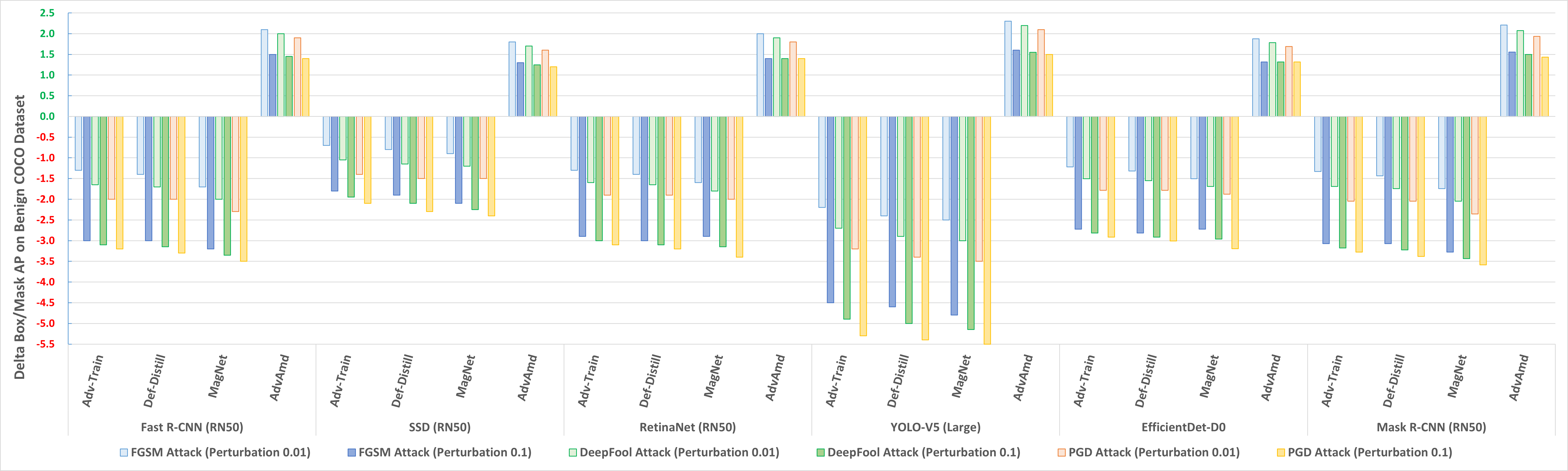
Figure 3: Comparison on benign COCO dataset. Only AdvAmd solves the accuracy degradation. (The variance is within $\pm$0.07 for box/mask AP with different random seeds.)

Compared to the prior art of the adversarial defense methods with negative delta metrics, only the AdvAmd method solves the accuracy degradation on the benign dataset. With all three adversarial attacks, AdvAmd method has better accuracy boosting performance when the adversarial perturbation is lower. Because the more significant perturbations lead to more severe distribution drift and mismatch between the adversarial and benign samples.

5.4 Comparison Experiments on Adversarial Set

To confirm whether AdvAmd method is still effective as a defense strategy, we repeat the same experiment setting as the previous section, while testing the corresponding accuracy on the adversarial attacked ImageNet and COCO dataset. To be clearer, only the delta Top-1 accuracy and box/mask average precision metrics are shown in Figure 4 and Figure 5.

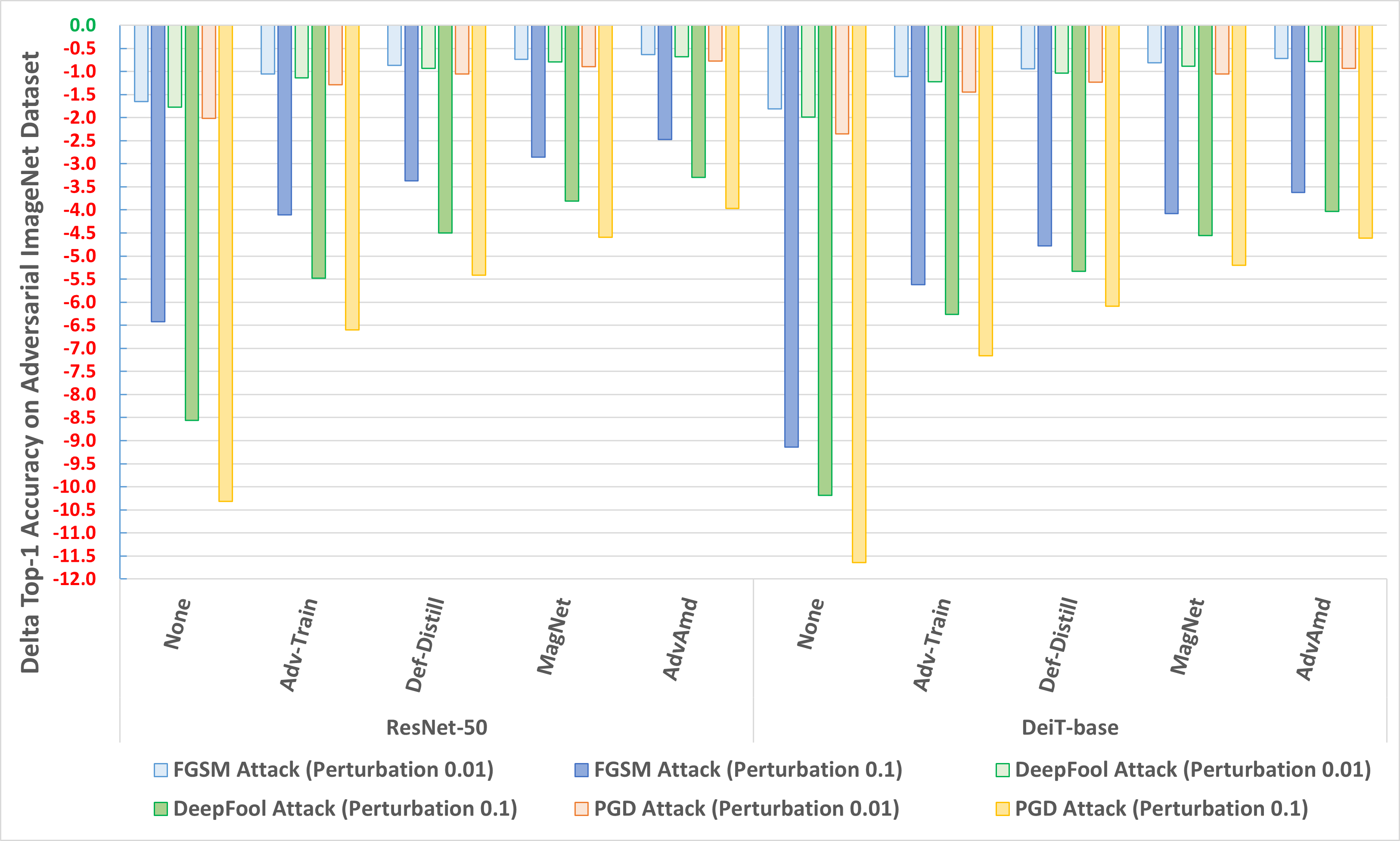
Figure 4: Results on adversarial ImageNet dataset. AdvAmd remains the adversarial defense capability. (The variance is within $\pm$0.06 for Top-1 with different random seeds.)

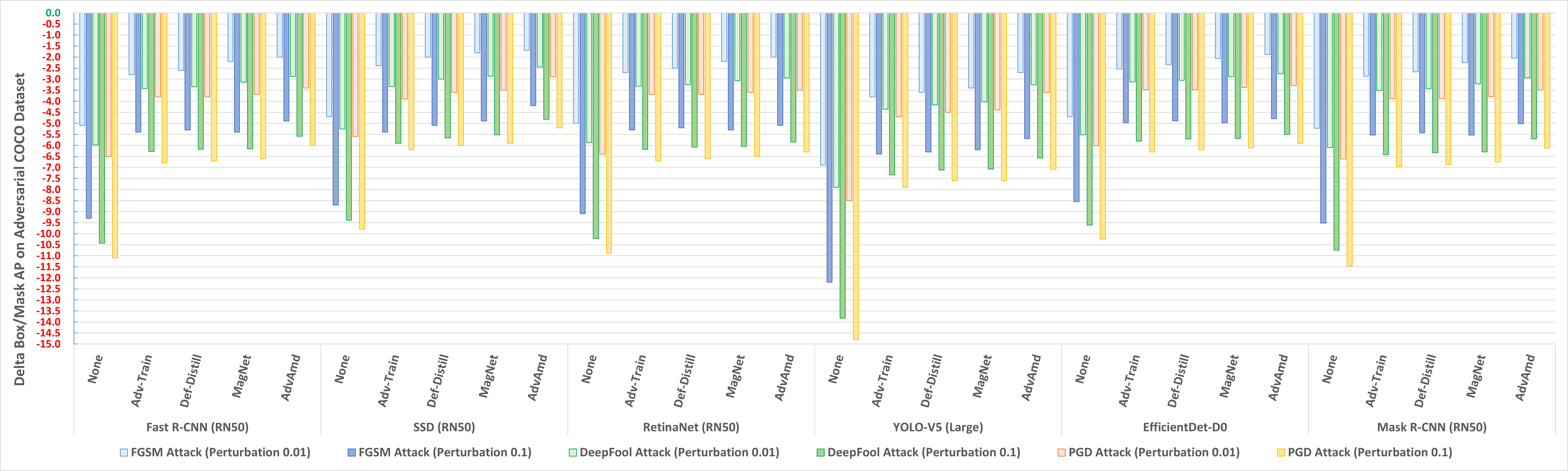
Figure 5: Results on adversarial COCO dataset. AdvAmd remains the adversarial defense capability. (The variance is within $\pm$0.15 for box/mask AP with different random seeds.)

Compared to the metrics degradation on the adversarial dataset without adversarial defense involved, the AdvAmd method and the prior art of the adversarial defense methods, can compensate and reduce the accuracy gap. That proves the AdvAmd method can still defend the adversarial attacks and improve the adversarial robustness of the neural models. By decreasing the distribution mismatch between the benign and adversarial samples and disentangling the mutual learning with an auxiliary BN mechanism, the judgment distribution of the amended model is more centralized to the mean of each category. So the vague regions between the adjacent categories will be reduced. That’s why AdvAmd can maintain good performance as an adversarial defense strategy.

5.5 Ablation Experiments and Insights

In this experiment, we want to check the contribution of each key component in AdvAmd to the final accuracy boosting performance on the benign dataset, as well as the adversarial defense efficacy. Then we can have a deep insight into why AdvAmd can harness and transfer the adversarial attack and whether we can further improve it. We include three key components which may have an apparent potential contribution, i.e., the utilization of 1. mediate samples, 2. auxiliary BN, 3. AdvAmd loss.

Network	Mediate Samples	Auxiliary Batch Norm	AdvAmd Loss	$\Delta$ Mask/Box AP on Adversarial Dataset				$\Delta$ Mask/Box AP on Benign Dataset
				FGSM Attack		PGD Attack		FGSM Attack		PGD Attack
				$\epsilon$=0.01	$\epsilon$=0.1	$\epsilon$=0.01	$\epsilon$=0.1	$\epsilon$=0.01	$\epsilon$=0.1	$\epsilon$=0.01	$\epsilon$=0.1
DeiT-base	✓	✗	✗	-1.6	-7.2	-2.1	-9.2	-1.3	-2.6	-2.8	-3.6
	✗	✓	✗	-1.4	-7.1	-1.9	-8.7	0.4	0.1	0.3	0.1
	✗	✗	✓	-1.4	-7.0	-1.8	-8.5	0.5	0.2	0.4	0.1
	✓	✓	✗	-1.2	-4.2	-1.5	-5.3	1.4	0.8	1.1	0.6
	✓	✗	✓	-1.2	-4.1	-1.4	-5.2	1.5	0.9	1.2	0.7
	✗	✓	✓	-1.1	-3.9	-1.2	-4.8	2.3	1.6	1.8	1.2
	✓	✓	✓	-0.7	-3.6	-0.9	-4.6	2.5	1.8	1.9	1.5
Mask R-CNN (RN50)	✓	✗	✗	-3.0	-6.1	-4.9	-7.5	-2.4	-4.8	-3.3	-5.4
	✗	✓	✗	-2.6	-5.5	-4.3	-6.7	-0.1	-1.0	-0.3	-1.1
	✗	✗	✓	-2.6	-5.6	-4.4	-6.9	-0.1	-1.1	-0.3	-1.2
	✓	✓	✗	-2.3	-5.4	-3.8	-6.3	1.2	0.2	1.0	0.2
	✓	✗	✓	-2.4	-5.4	-4.0	-6.5	1.1	0.1	0.9	0.1
	✗	✓	✓	-2.2	-5.3	-3.8	-6.4	1.9	1.3	1.7	1.2
	✓	✓	✓	-2.0	-5.0	-3.5	-6.1	2.2	1.6	1.9	1.4
YOLO-V5 (Large)	✓	✗	✗	-3.6	-6.5	-4.6	-8.0	-2.6	-5.0	-3.7	-5.8
	✗	✓	✗	-3.3	-6.1	-4.2	-7.7	0.1	-1.0	-0.3	-1.2
	✗	✗	✓	-3.4	-6.3	-4.4	-7.9	0.1	-1.2	-0.4	-1.4
	✓	✓	✗	-3.0	-5.9	-3.9	-7.4	1.2	0.2	1.0	0.1
	✓	✗	✓	-3.1	-6.0	-4.1	-7.6	1.0	0.1	0.7	0.0
	✗	✓	✓	-3.0	-5.9	-3.9	-7.3	1.9	1.3	1.8	1.2
	✓	✓	✓	-2.7	-5.7	-3.6	-7.1	2.3	1.6	2.1	1.5

Table 3: Ablation experiment to check the contribution of key components in AdvAmd method on detection task.

We make the combination to enable or disable among three key components. The ablation results are shown in Table 3. Suppose we only apply the AdvAmd method with the lacking of one key component. In that case, we can find the absence of the mediate samples has about $\textbf{0.1\%}\sim\textbf{0.3\%}$ decrease of Top-1 accuracy for DeiT-base, $\textbf{0.2\%}\sim\textbf{0.3\%}$ decrease of the mask AP for Mask R-CNN and $\textbf{0.3\%}\sim\textbf{0.4\%}$ decrease of the box AP for YOLO-V5 on the benign dataset, while the absence of the utilization of the auxiliary BN or AdvAmd loss has around $\textbf{0.7\%}\sim\textbf{1.1\%}$ Top-1 accuracy decrease for DeiT-base, $\textbf{1.1\%}\sim\textbf{1.5\%}$ mask accuracy decrease for Mask R-CNN and $\textbf{1.1\%}\sim\textbf{1.5\%}$ box accuracy decrease for YOLO-V5 on the benign dataset. It seems that the contribution of the mediate samples is less than the other two components. We further verify the ablation results with the AdvAmd method, which only applies one of the key components. If only enabling the mediate samples for the AdvAmd method, the accuracy degradation on the benign dataset is still severe. While applying one of the auxiliary BN or AdvAmd loss, the accuracy degradation will be healed. The delta box AP on the benign dataset between the amended and vanilla target models is close to zero for the adversarial attack with minor perturbations. So we can confirm that the auxiliary BN and AdvAmd loss are two powerful improvements to heal the accuracy degradation on the benign dataset. However, we should notice that if the utilization of the mediate samples is enabled with one of the auxiliary BN or AdvAmd loss, there is an obvious accuracy boost. That proves the separate utilization of the mediate samples can help in a relatively small margin. While at the same time, the combination utilization of the mediate samples with the other two amendment components can also help in a relatively large margin.

On the other hand, the lacking of one or two key components only leads to a limited negative influence on the defense performance on the adversarial dataset. These three key components are designed to solve the accuracy degradation of the benign dataset caused by distribution mismatch and mutual learning, so the limited influence on the defense efficacy is not surprising. Moreover, the prior art defense strategy’s principle is teaching the target model that the adversarial samples in the vague judgment range can still be regarded as the normal samples. While the key components introduced in AdvAmd teach the amended model to judge the benign, mediate, and adversarial samples in finer granularity. From the results on the adversarial dataset, the finer-granularity division for these samples can only provide some but limited help for the adversarial defense efficacy. It reveals an interesting conclusion that the finer granularity uses a sled-hammer on a gnat for adversarial defense task.

6 Limitations and Future Work

In the AdvAmd method, we mainly consider the adversarial attack pattern to mislead the models in categories detection and classification. Although this is the prior art attack strategy, whether the AdvAmd method can also help to harness the attack aiming at confusing the detected and segmented positions has not been demonstrated. We leave it for further study in the future work.

7 Conclusions

We notice the prior art adversarial defense methods lead to accuracy degradation of the classification, object detection and segmentation models on the benign dataset. Based on the qualitative explanation and theoretical proof, we find the distribution mismatch between the benign and adversarial samples and the mutual learning mechanism with same learning ratio applied in prior art adversarial defense strategies is the root cause. Then we propose the AdvAmd method to harness the adversarial attack for healing the accuracy degradation. Three key components: mediate samples (to reduce the influence of distribution mismatch with a fine-grained amendment), auxiliary batch norm (to solve the mutual learning mechanism and the smoother judgment surface), and AdvAmd loss (to adjust the learning ratios according to different attack vulnerabilities) make the main contribution to amending the adversarial attack in the right manner.

Ethical Statement

We should emphasize the aim of AdvAmd is transferring and healing the adversarial attacks’ influence on various classification and object detection tasks. However, we encourage the community to understand and mitigate the risks arising from the AdvAmd method. As the principle and the implementation of AdvAmd will be public, people may study the novel adversarial attack to deactivate the AdvAmd intentionally. We should notice the risk that AdvAmd is misused to help evolve more powerful attacks that can be used to misrepresent objective truth.

References

- Belinkov and Bisk [2017] Yonatan Belinkov and Yonatan Bisk. Synthetic and natural noise both break neural machine translation. arXiv preprint arXiv:1711.02173, 2017.
- Cisse et al. [2017] Moustapha M Cisse, Yossi Adi, Natalia Neverova, and Joseph Keshet. Houdini: Fooling deep structured visual and speech recognition models with adversarial examples. Advances in Neural Information Processing Systems, 30, 2017.
- Deng et al. [2009] Jia Deng, Wei Dong, Richard Socher, Li-Jia Li, Kai Li, and Li Fei-Fei. Imagenet: A large-scale hierarchical image database. In 2009 IEEE conference on computer vision and pattern recognition, pages 248–255. IEEE, 2009.
- Dziugaite et al. [2016] Gintare Karolina Dziugaite, Zoubin Ghahramani, and Daniel M Roy. A study of the effect of jpg compression on adversarial images. arXiv preprint arXiv:1608.00853, 2016.
- Goodfellow et al. [2014] Ian J Goodfellow, Jonathon Shlens, and Christian Szegedy. Explaining and harnessing adversarial examples. arXiv preprint arXiv:1412.6572, 2014.
- He et al. [2016] Kaiming He, Xiangyu Zhang, Shaoqing Ren, and Jian Sun. Deep residual learning for image recognition. In Proceedings of the IEEE conference on computer vision and pattern recognition, pages 770–778, 2016.
- He et al. [2017] Kaiming He, Georgia Gkioxari, Piotr Dollár, and Ross Girshick. Mask r-cnn. In Proceedings of the IEEE International Conference on Computer Vision, pages 2961–2969, 2017.
- Hinton et al. [2015] Geoffrey Hinton, Oriol Vinyals, and Jeff Dean. Distilling the knowledge in a neural network. arXiv preprint arXiv:1503.02531, 2015.
- Huang et al. [2015] Ruitong Huang, Bing Xu, Dale Schuurmans, and Csaba Szepesvári. Learning with a strong adversary. arXiv preprint arXiv:1511.03034, 2015.
- Ioffe and Szegedy [2015] Sergey Ioffe and Christian Szegedy. Batch normalization: Accelerating deep network training by reducing internal covariate shift. In International Conference on Machine Learning, pages 448–456. PMLR, 2015.
- Jocher [2022] Glenn Jocher. ultralytics/yolov5: v6.1 - TensorRT, TensorFlow Edge TPU and OpenVINO Export and Inference, February 2022.
- Kurakin et al. [2016] Alexey Kurakin, Ian Goodfellow, and Samy Bengio. Adversarial machine learning at scale. arXiv preprint arXiv:1611.01236, 2016.
- Liang et al. [2017] Bin Liang, Hongcheng Li, Miaoqiang Su, Pan Bian, Xirong Li, and Wenchang Shi. Deep text classification can be fooled. arXiv preprint arXiv:1704.08006, 2017.
- Lin et al. [2014] Tsung-Yi Lin, Michael Maire, Serge Belongie, James Hays, Pietro Perona, Deva Ramanan, Piotr Dollár, and C Lawrence Zitnick. Microsoft coco: Common objects in context. In European Conference on Computer Vision, pages 740–755. Springer, 2014.
- Lin et al. [2017] Tsung-Yi Lin, Priya Goyal, Ross Girshick, Kaiming He, and Piotr Dollár. Focal loss for dense object detection. In Proceedings of the IEEE International Conference on Computer Vision, pages 2980–2988, 2017.
- Liu et al. [2016] Wei Liu, Dragomir Anguelov, Dumitru Erhan, Christian Szegedy, Scott Reed, Cheng-Yang Fu, and Alexander C Berg. Ssd: Single shot multibox detector. In European Conference on Computer Vision, pages 21–37. Springer, 2016.
- Lyu et al. [2015] Chunchuan Lyu, Kaizhu Huang, and Hai-Ning Liang. A unified gradient regularization family for adversarial examples. In 2015 IEEE International Conference on Data Mining, pages 301–309. IEEE, 2015.
- Madry et al. [2018] Aleksander Madry, Aleksandar Makelov, Ludwig Schmidt, Dimitris Tsipras, and Adrian Vladu. Towards deep learning models resistant to adversarial attacks. In International Conference on Learning Representations, 2018.
- Meng and Chen [2017] Dongyu Meng and Hao Chen. Magnet: a two-pronged defense against adversarial examples. In Proceedings of the 2017 ACM SIGSAC Conference on Computer and Communications Security, pages 135–147, 2017.
- Mirjalili and Ross [2017] Vahid Mirjalili and Arun Ross. Soft biometric privacy: Retaining biometric utility of face images while perturbing gender. In 2017 IEEE International Joint Conference on Biometrics, pages 564–573. IEEE, 2017.
- Moosavi-Dezfooli et al. [2016] Seyed-Mohsen Moosavi-Dezfooli, Alhussein Fawzi, and Pascal Frossard. Deepfool: a simple and accurate method to fool deep neural networks. In Proceedings of the IEEE/CVF Conference on Computer Vision and Pattern Recognition, pages 2574–2582, 2016.
- Nadarajah and Pogány [2016] Saralees Nadarajah and Tibor K Pogány. On the distribution of the product of correlated normal random variables. Comptes Rendus Mathematique, 354(2):201–204, 2016.
- NVIDIA A100 [2020] NVIDIA A100. NVIDIA A100 Tensor Core GPU Architecture, 2020.
- NVIDIA V100 [2017] NVIDIA V100. NVIDIA Tesla V100 GPU Architecture, 2017.
- Ozdag [2018] Mesut Ozdag. Adversarial attacks and defenses against deep neural networks: a survey. Procedia Computer Science, 140:152–161, 2018.
- Papernot and McDaniel [2017] Nicolas Papernot and Patrick McDaniel. Extending defensive distillation. arXiv preprint arXiv:1705.05264, 2017.
- Papernot et al. [2016] Nicolas Papernot, Patrick McDaniel, Xi Wu, Somesh Jha, and Ananthram Swami. Distillation as a defense to adversarial perturbations against deep neural networks. In 2016 IEEE Symposium on Security and Privacy, pages 582–597. IEEE, 2016.
- Paszke et al. [2017] Adam Paszke, Sam Gross, Soumith Chintala, Gregory Chanan, Edward Yang, Zachary DeVito, Zeming Lin, Alban Desmaison, Luca Antiga, and Adam Lerer. Automatic differentiation in pytorch. In Advances in Neural Information Processing Systems-Autodiff Workshop, 2017.
- Ren et al. [2015] Shaoqing Ren, Kaiming He, Ross Girshick, and Jian Sun. Faster r-cnn: Towards real-time object detection with region proposal networks. Advances in Neural Information Processing Systems, 28, 2015.
- Samangouei et al. [2018] Pouya Samangouei, Maya Kabkab, and Rama Chellappa. Defense-gan: Protecting classifiers against adversarial attacks using generative models. arXiv preprint arXiv:1805.06605, 2018.
- Szegedy et al. [2013] Christian Szegedy, Wojciech Zaremba, Ilya Sutskever, Joan Bruna, Dumitru Erhan, Ian Goodfellow, and Rob Fergus. Intriguing properties of neural networks. arXiv preprint arXiv:1312.6199, 2013.
- Tan et al. [2020] Mingxing Tan, Ruoming Pang, and Quoc V Le. Efficientdet: Scalable and efficient object detection. In Proceedings of the IEEE/CVF conference on computer vision and pattern recognition, pages 10781–10790, 2020.
- Touvron et al. [2021] Hugo Touvron, Matthieu Cord, Matthijs Douze, Francisco Massa, Alexandre Sablayrolles, and Hervé Jégou. Training data-efficient image transformers & distillation through attention. In International Conference on Machine Learning, pages 10347–10357. PMLR, 2021.
- Tramèr et al. [2017] Florian Tramèr, Alexey Kurakin, Nicolas Papernot, Ian Goodfellow, Dan Boneh, and Patrick McDaniel. Ensemble adversarial training: Attacks and defenses. arXiv preprint arXiv:1705.07204, 2017.
- Xie et al. [2019] Cihang Xie, Yuxin Wu, Laurens van der Maaten, Alan L Yuille, and Kaiming He. Feature denoising for improving adversarial robustness. In Proceedings of the IEEE/CVF Conference on Computer Vision and Pattern Recognition, pages 501–509, 2019.
- Xu et al. [2020] Xing Xu, Jingran Zhang, Yujie Li, Yichuan Wang, Yang Yang, and Heng Tao Shen. Adversarial attack against urban scene segmentation for autonomous vehicles. IEEE Transactions on Industrial Informatics, 17(6):4117–4126, 2020.
- Zhang et al. [2020] Ziqi Zhang, Xinge Zhu, Yingwei Li, Xiangqun Chen, and Yao Guo. Adversarial attacks on monocular depth estimation. arXiv preprint arXiv:2003.10315, 2020.