Multi-resolution Spatiotemporal Enhanced Transformer Denoising with Functional Diffusive GANs for Constructing Brain Effective Connectivity in MCI analysis

Abstract

Effective connectivity can describe the causal patterns among brain regions. These patterns have the potential to reveal the pathological mechanism and promote early diagnosis and effective drug development for cognitive disease. However, the current studies mainly focus on using empirical functional time series to calculate effective connections, which may not comprehensively capture the complex causal relationships between brain regions. In this paper, a novel Multi-resolution Spatiotemporal Enhanced Transformer Denoising (MSETD) network with an adversarially functional diffusion model is proposed to map functional magnetic resonance imaging (fMRI) into effective connectivity for mild cognitive impairment (MCI) analysis. To be specific, the denoising framework leverages a conditional diffusion process that progressively translates the noise and conditioning fMRI to effective connectivity in an end-to-end manner. To ensure reverse diffusion quality and diversity, the multi-resolution enhanced transformer generator is designed to extract local and global spatiotemporal features. Furthermore, a multi-scale diffusive transformer discriminator is devised to capture the temporal patterns at different scales for generation stability. Evaluations of the ADNI datasets demonstrate the feasibility and efficacy of the proposed model. The proposed model not only achieves superior prediction performance compared with other competing methods but also identifies MCI-related causal connections that are consistent with clinical studies.

I Introduction

Brain effective connectivity (BEC) describes the causal interaction from one brain region to another and helps perform various cognitive and perceptual tasks [1]. It aims to transmit and analyze functional information between distant regions of the brain for improving the brain’s information processing speed and accuracy [2]. Recent studies have shown that the abnormal topological changes of BEC can reflect the underlying pathology of brain disease [3, 4]. These changes are probably accompanied by alterations in the brain’s microstructure [5, 6], such as those associated with Alzheimer’s disease (AD) and its early-stage mild cognitive impairment (MCI). Investigation of the BEC is able to better understand the underlying mechanisms associated with neurodegenerative diseases and develop potential treatments or new drugs for rehabilitation [7, 8]. Therefore, constructing BEC from functional magnetic resonance imaging (fMRI) becomes a very promising way to analyze cognitive disease and identify possible biomarkers for MCI diagnosis.

Constructing BEC involves learning a mapping network to predict directional connectivities from one neural unit to another by analyzing their functional signals. Since the fMRI has the advantages of being noninvasive and having high temporal resolution, it has drawn great attention in exploring the complex connectivity features for cognitive disease diagnosis [9, 10, 11]. The brain functional connectivity (BFC) gives the temporal correlation between any pair of neural units, while the BEC is an asymmetric matrix representing the directional information of neural transmission. The directed graph can be used to analyze BEC, including a set of vertices (named regions-of-interest, or ROIs) and a set of directed edges (effective connections). Previous researchers focused on BEC learning by using traditional learning methods, including the dynamic causal models (DCM) [12], the Bayesian network (BN) method [13], the correlation analysis method [14], and so on. These methods utilize shallow network structure or prior knowledge and are unable to extract complex connectivity features from fMRI, which may bring about inaccuracies in BECs and deduce low performance in disease analysis.

Recently, deep learning methods have been widely applied in the exploration of BEC learning [15, 16]. It not only achieves quite a good performance on image recognition tasks in Euclidean space but also shows excellent results on brain network generation in non-Euclidean space. The primary characteristic is the strong ability to perform high-level and complex feature extraction. Increasingly new methods based on deep learning have been explored to construct BEC from functional MRI data [17, 18]. However, the current methods heavily rely on the software toolkit to preprocess the fMRI before extracting empirical time-series data. The main drawback is that the manual parameter settings of these preprocessing procedures may result in large errors by different researchers.

As the most popular and powerful generative model, the generative adversarial network (GAN) [19] implicitly characterizes the distribution of synthetic samples through a two-player adversarial game. It can generate high-quality samples with efficient computation while producing homogeneous samples because of training instability and mode collapse. An alternative way to solve this issue is the emergence of diffusion denoising probabilistic models (DDPM) [20] that have received great attention in generating tasks [21, 22, 23]. The main advantage is the great generating ability for high-quality and diverse samples, and the disadvantage lies in the expensive computation. Inspired by the above observations, we combine the advantages of the GAN and the DDPM to improve generation performance. The novel multi-resolution spatiotemporal enhanced transformer denoising (MSETD) model is proposed to learn brain effective connectivity from the 4D fMRI for mild cognitive impairment (MCI) analysis. Specifically, the 4D fMRI is first transformed to ROI time-series features (also called a rough sample) by introducing an anatomical segmentation mask, and the rough sample is then treated as conditioning to gradually denoise the Gaussian sample and generate clean samples. Next, by splitting the generation processes into a few steps, adversarial learning is more stable and gets rid of mode collapse. Besides, the designed generator can capture hierarchical spatial-temporal features and enhance clean sample generation. Finally, the estimated BEC from the generators reflects a more sophisticated causal relationship between brain regions and captures the prominent MCI-related features. To the best of our knowledge, the proposed MSETD is the first work to translate 4D fMRI into BEC in an end-to-end manner using functional diffusive GANs. The main contributions of this work are summarized as follows:

• The proposed functional MSETD model is the first work that generates BEC from 4D fMRI in an end-to-end manner. It separates the diffusion denoising process into several successive steps and leverages the generative adversarial strategy to gradually translate the noise and conditioning fMRI into effective connectivity, which makes the generation process high-quality, diverse, and efficient.

• The hierarchical hybrid enhanced transformer generator is designed to denoise the fMRI by first paying attention to global spatial connectivity features and then focusing on local temporal characteristics. The multi-scale spatiotemporal features are significantly enhanced, and the denoise quality is greatly improved.

• The multi-resolution diffusive transformer discriminator is devised to capture the temporal patterns of the denoised fMRI at different scales, which ensures the denoising process is stable and the generation result is diverse.

The rest of this paper is structured as follows: The related works are introduced in Section II. The overall architecture of the proposed MSETD model is presented in Section III. The experimental results, including generation evaluation and classification performance, are described in Section IV. The reliability of our results is discussed in Section V, and Sections VI draw the main conclusions.

II Related Work

II-A BEC learning methods

Functional connectivity network analysis is usually used to identify abnormal connectivity patterns that are associated with different cognitive functions, such as memory, attention, and emotion. The BEC belongs to the functional connectivity network and can bridge causal connections between brain regions. Many studies have focused on exploring the BEC for better diagnostic performance and good interpretability. There are two categories of methods for learning BEC from functional data: shallow learning methods and deep learning methods.

The frequently used shallow method is the dynamic causal model (DCM)[12]. For example, Park et al.[24] employed the parametric empirical Bayes method to model the directed effects of sliding windows. And the Granger causality (GC)[25, 26] is the most commonly used shallow method. For example, DSouza et al. [27] utilize the multiple regression algorithm to process historical information from functional time series for causal interaction prediction. These methods cannot extract deep and complex connectivity features from fMRI.

To explore the deep features of fMRI, deep learning methods show great success in causal modeling between brain regions. The work in [28] employed nonlinear causal relationship estimation with an artificial neural network to predict causal relations between brain regions by analyzing both linear and nonlinear components of EEG data. Also, Abbasvandi et al.[29] combined the recurrent neural network and Granger causality to estimate effective connectivity from EEG data. They greatly improved the prediction accuracy of simulation data and the epileptic seizures dataset. Considering the great ability of GANs to characterize data distribution, Liu et al.[30] designed a GAN-based network to infer directed connections from fMRI data. To capture temporal features, they[31] employed recurrent generative adversarial networks for effective connectivity learning. Presently, Zou et al.[32] introduced the graph convolutional network (GCN) to mine both temporal and spatial topological relationships among distant brain regions for learning BECs. Although the above deep learning methods achieved promising prediction performance in BEC estimation, they heavily rely on the software toolkit to preprocess the fMRI for extracting empirical time-series data. That may result in large errors due to different manual parameter settings during preprocessing procedures.

II-B Generative learning models

Generative adversarial networks (GANs) have ruled generative approaches since they were first proposed by Goodfellow. The primary advantage is implicitly modeling the distribution of the generated data through a two-player game. Many variants of GANs have been proposed and applied to many generation tasks[33, 34, 35], such as generating super-resolution, synthesizing cross-modal data, segmenting images, and so on. To satisfy specific generating tasks, conditional GAN[36] and related variants also achieve quite good performance efficiently[37]. The problem of instability and mode collapse in training has not been completely addressed yet. This may lead to homogeneously generated data and hinder its wider applications. Recently, denoising diffusion probabilistic models (DDPM) have attracted much attention in image generation [38, 39, 40] because of their ability to generate high-quality and diverse results. DDPM aims to denoise the noisy Gaussian data gradually and recover the clean data. However, the denoising process requires a Gaussian distribution assumption with only a small denoising step, which leads to slow reverse diffusion in about thousands of steps to approach clean data. Based on the above observations, we try to combine the advantages of GAN and DDPM in generation, such as efficiency, high quality, and diversity. We propose the novel MSETD model to precisely learn BEC from 4D fMRI for MCI analysis.

Figure 1: The architecture of the proposed denoising model. In the forward process, the empirical sample $F_{0}$ is transformed to the normal Gaussian noisy sample $F_{T}$ by gradually adding noise. In the reverse process, the rough sample $X$ is considered as conditioning input to guide the generator $G_{\theta}$ in synthesizing the denoised sample $F_{0}^{\prime}$ from $F_{T}$; meanwhile, a discriminator $D_{\theta}$ distinguishes the actual or synthesized sample for the denoising optimization.

III Method

The proposed MSETD model jointly leverages denoising diffusion probabilistic models (DDPM) and generative adversarial networks (GANs) to translate a 4-dimensional fMRI into a one-dimensional time series and construct brain effective connectivities (BEC) for MCI analysis. To be specific, the fMRI is mapped into a one-dimensional time series (called the rough sample $\mathbf{X}$) of N ROIs by incorporating the anatomical atlas mask. The rough sample guides the diffusion model to translate the gaussian noise into a clean sample using conditional diffusion models. We first introduce conventional diffusion models and then describe functional diffusive GANs with transformer-based generators and discriminators. Finally, hybrid objectives are devised to ensure effective diffusion and generate high-quality samples efficiently.

III-A Conventional Denoising Diffusion Model

The basic principle of the diffusion model is to learn the information attenuation caused by noise and then use the learned patterns to generate denoised data. It is usually divided into the forward process and the inverse process. In the diffusion process, Gaussian noise is constantly added to the input sample $F_{0}$ for sufficiently large $T$ (hundreds or thousands) steps. Under the rules of the Markov chain, the probability distribution of a noisy sample $F_{T}$ will approach the stationary distribution (such as the Gaussian distribution) at the $T$-th step. Here is the diffusion formula:

$$q\left(\mathbf{F}_{1:T}\mid\mathbf{F}_{0}\right)=\prod_{t=1}^{T}q\left(\mathbf{F}_{t}\mid\mathbf{F}_{t-1}\right)$$ (1)

$$q\left(\mathbf{F}_{t}\mid\mathbf{F}_{t-1}\right)=\mathcal{N}\left(\mathbf{F}_{t};\sqrt{1-\beta_{t}}\mathbf{F}_{t-1},\beta_{t}\mathbf{I}\right)$$ (2)

where $t=\{1,2,...,T\}$. $\beta_{t}$ is the noise variance that is defined before the model’s training. $\mathcal{N}$ is the assumed Gaussian distribution, and $\mathbf{I}$ is an identity matrix. The reverse process also follows the Markov chain to translate the noisy sample $F_{T}$ to a cleaned sample $F_{0}$. The assumption of a large step $T$ and a small $\beta_{t}$ can model the denoising probability in a Gaussian distribution:

$$p_{\theta}\left(\mathbf{F}_{0:T}\right)=p\left(\mathbf{F}_{T}\right)\prod_{t=1}^{T}p_{\theta}\left(\mathbf{F}_{t-1}\mid\mathbf{F}_{t}\right)$$ (3)

$$p_{\theta}\left(\mathbf{F}_{t-1}\mid\mathbf{F}_{t}\right)=\mathcal{N}\left(\mathbf{F}_{t-1};\bm{\mu}_{\theta}\left(\mathbf{F}_{t},t\right),\sigma_{t}^{2}\mathbf{I}\right)$$ (4)

where $\bm{\mu}_{\theta}(\mathbf{F}_{t},t)$ and $\sigma_{t}^{2}$ are the mean and variance of the denoised sample $\mathbf{F}_{t-1}$. $\theta$ indicates the network’s parameters.

We use the deep learning model $p_{\theta}(\mathbf{F}_{t-1}|\mathbf{F}_{t})$ to approximate the true distribution $q(\mathbf{F}_{t-1}|\mathbf{F}_{t})$, and get the reparameterization of $\mu$ and $\sigma_{t}^{2}$ in the following form:

$$\bm{\mu}_{\theta}\left(\mathbf{F}_{t},t\right)=\frac{1}{\sqrt{\alpha_{t}}}\left(\mathbf{F}_{t}-\frac{\beta_{t}}{\sqrt{1-\bar{\alpha}_{t}}}\bm{\epsilon}_{\theta}\left(\mathbf{F}_{t},t\right)\right)$$ (5)

$$\sigma_{t}^{2}=\frac{\left(1-\bar{\alpha}_{t-1}\right)}{\left(1-\bar{\alpha}_{t}\right)}\beta_{t}$$ (6)

here, $\alpha_{t}=1-\beta_{t},\bar{\alpha}_{t}=\prod_{i=1}^{t}\alpha_{i}$. By applying a variational evidence lower bound (ELBO) constraint, the added noise $\bm{\epsilon}_{\theta}(\mathbf{F}_{t},t))$ can be calculated by minimizing the MSE loss:

$$\mathbb{E}_{t,\mathbf{F}_{0},\bm{\epsilon}}\left[\left\|\bm{\epsilon}-\bm{\epsilon}_{\theta}\left(\sqrt{\bar{\alpha}_{t}}\mathbf{F}_{0}+\sqrt{1-\bar{\alpha}_{t}}\bm{\epsilon},t\right)\right\|^{2}\right]$$ (7)

where, $\bm{\epsilon}\sim\mathcal{N}(\mathbf{0},\mathbf{I})$. After the model’s optimization, new samples can be derived from Gaussian noise $F_{T}\sim\mathcal{N}(\mathbf{0},\mathbf{I})$ by gradually reversing diffusing $T$ steps based on Eq.( 3) and Eq.( 4).

III-B Functional diffusive GANs

Conventional DDPM can generate high-quality samples but suffers from low efficiency in sampling because of the thousands of denoising steps. While the GAN can make up for this shortcoming by having fast-generating ability, Thus, we propose novel functional diffusive GANs by combining both of them for efficient and high-fidelity sampling generation. Apart from this, there are two other differences compared with the conventional DDPM: (a) A rough sample is treated as conditioning to guide the denoising process. Since our goal is to denoise the rough sample $\mathbf{X}$ into a clean subject-specific sample $\mathbf{F}_{0}$, the unconditional diffusion process likely generates diverse samples that cannot reflect subject-specific disease information; (2) the step size is reduced by a factor of $s$ ($s>>1$), which speeds the generation process and keeps the sample in high quality.

III-B1 Functional diffusion process

The proposed diffusive GANs divide the denoising process into a few steps by using generative adversarial networks, where each step is conditioned by a rough sample to make the process easy to learn. It should be stressed that our model advantages DDPM in efficiency and high-fidelity denoising, diminishing the training instability and mode collapse encountered at GANs optimization. As shown in Fig. 1, it consists of two parts: the forward process from the empirical sample to the Gaussian noisy sample and the reverse process from the Gaussian noisy sample to the empirical sample conditioned on the rough sample.

In the forward direction, the empirical sample $\mathbf{F}_{0}$ is transformed to the normal Gaussian noisy sample $\mathbf{F}_{T}$ by gradually adding noise. The computation formula is the same as Eq.( 2). In the reverse direction, we should consider the condition $\mathbf{X}$ in the denoising procedure. First, the rough sample $\mathbf{X}$ is considered as conditioning input to guide the generator $\mathbf{G}_{\theta}$ predict the initial sample $\mathbf{\hat{F}}_{0}$ from $\mathbf{F}_{T}$, then the posterior sampling is utilized to synthesize the denoised sample $\mathbf{F}_{t-s}^{\prime}$; meanwhile, the multi-resolution diffusive transformer discriminator $\mathbf{D}_{\theta}$ distinguishes the actual ($\mathbf{F}_{t-s}$) or synthetic ($\mathbf{F}_{t-s}^{\prime}$) for the denoising process. Specifically, at the $t$ step, we aim to predicte $\mathbf{F}_{t-s}$ from $\mathbf{F}_{t}$. Firstly, a generator $\mathbf{G}_{\theta}(\mathbf{F}_{t},\mathbf{X},t)$ is utilized to predict the initial sample $\mathbf{\hat{F}}_{0}^{[t/s]}$, then $\mathbf{F}_{t-s}$ is sampled using the posterior distribution $q(\mathbf{F}_{t-s}|\mathbf{F}_{t},\mathbf{\hat{F}}_{0}^{[t/s]})$ by giving $\mathbf{F}_{t}$ and $\mathbf{\hat{F}}_{0}^{[t/s]}$. Finally, after $T/s$ steps, the ultimate denoised sample $\mathbf{F}_{0}^{\prime}$ (equal to $\mathbf{\hat{F}}_{0}^{[1]}$) sampled from the estimated distribution $p_{\theta}(\mathbf{F}_{0}\mid\mathbf{F}_{s},\mathbf{X})$. The denoising process can be expressed as follows:

Figure 2: The structure of the multi-channel adaptor. The inputs are the noisy sample $\mathbf{F}_{t}$ and the rough sample $\mathbf{X}$, and the output is the fused sample. The three samples share the same dimension.

Figure 3: The detailed structure of the SeTe block. The input and output share the same dimension. It passes successively through the spatial multi-head attention module and the temporal multi-head attention module.

$$p_{\theta}\left(\mathbf{F}_{t-s}\mid\mathbf{F}_{t},\mathbf{X}\right):=q\left(\mathbf{F}_{t-s}\mid\mathbf{F}_{t},\hat{\mathbf{F}}_{0}^{[t/s]}=\mathbf{G}_{\theta}^{[t/s]}\left(\mathbf{F}_{t},\mathbf{X},t\right)\right)$$ (8)

$$q\left(\mathbf{F}_{t-s}\mid\mathbf{F}_{t},\hat{\mathbf{F}}_{0}^{[t/s]}\right)=q\left(\mathbf{F}_{t}\mid\mathbf{F}_{t-s},\hat{\mathbf{F}}_{0}^{[t/s]}\right)\frac{q\left(\mathbf{F}_{t-s}\mid\hat{\mathbf{F}}_{0}^{[t/s]}\right)}{q\left(\mathbf{F}_{t}\mid\hat{\mathbf{F}}_{0}^{[t/s]}\right)}$$ (9)

The sampling probability from $p_{\theta}\left(\mathbf{F}_{t-s}\mid\mathbf{F}_{t},\mathbf{X}\right)$ is defined as:

$$\mathbf{F}_{t-s}=\frac{\sqrt{\alpha_{t}}\left(1-\bar{\alpha}_{t-s}\right)}{1-\bar{\alpha}_{t}}\mathbf{F}_{t}+\frac{\sqrt{\bar{\alpha}_{t-s}}\beta_{t}}{1-\bar{\alpha}_{t}}\mathbf{G}_{\theta}^{[t/s]}+\bm{\epsilon}\sqrt{\beta_{t}}$$ (10)

III-B2 Hierarchical hybrid enhanced transformer generator

The aim of the hierarchical hybrid enhanced transformer generator ($\mathbf{G}_{\theta}$) is to remove the noise from noisy samples to obtain clean samples by conditioning guidance. Specifically, at $t$-the step, the input is the noisy sample $\mathbf{F}_{t}$ and the rough sample $\mathbf{X}$, and the output is the initial denoised sample $\mathbf{\hat{F}}_{0}$. All of them share the same size, $N\times d$. The generator consists of four modules, including the multi-channel adaptor (MCA), the spatial-enhanced temporal-enhanced (SeTe) blocks, the temporal down- and up-sampling (TDS and TUS), and the brain effective connectivity (BEC) estimator.

The MCA adaptively fuses the noisy sample $\mathbf{F}_{t}$ and the rough sample $\mathbf{X}$, Different from the traditional way of concatenating the two samples, we designed a cross-channel attention mechanism when fusing them. As shown in Fig. 2, first, the sample $\mathbf{F}_{t}$ is passed through the feed-forward network (FFN) and self-attention network; then, it is projected on the $\mathbf{X}$ to compute weighting scores for itself. We denote the input of cross-channel attention as $\mathbf{E}_{t}$ and $\mathbf{X}$, the output of this fusion operation can be expressed as follows:

$$\mathbf{E}_{t}^{\prime}=\operatorname{softmax}\left(\frac{\mathbf{E}_{t}\mathbf{X}^{T}}{\sqrt{d}}\right)\mathbf{E}_{t}$$ (11)

Next, the $1\times 3$ convolutional kernel is applied for each ROI to extract local features. Finally, FFN is used to adjust temporal features among different channels. The output of every sub-network has the same size, $N\times d$. The output of the MCA module is $\mathbf{F}_{t}^{MCA}$.

The TDS is used to halve the feature dimension and add the channels. Taking the first TDS as an example, for each ROI feature, we apply a 1D convolutional kernel with the size $1\times 3$ to extract local temporal features, and through $C$ convolutional kernels with a step size of $2$, each ROI feature is translated to a sequence of vectors with the length $d/2$. The final output $\mathbf{F}_{t}^{TDS}$ has the size $C\times N\times d/2$.

Figure 4: The structure of the BEC estimator. The outputs are a denoised sample and an asymmetric brain connectivity matrix.

The SeTe blocks are designed to extract both spatial and temporal features. The conventional transformed-based method focuses on the spatial correlation between pairs of ROIs while ignoring the temporal continuity. The SeTe benefits from multi-head attention (MSA), which enhances long-term dependence both spatially and temporally. As shown in Fig. 3, it is comprised of a spatial multi-head attention (SMA) and a temporal multi-head attention (TMA). The difference between these two attention networks is that the former is operated in the spatial direction, and the latter is operated in the temporal direction. The input is a tensor with the size $C\times N\times d/2$, and the output $\mathbf{F}_{t}^{SeTe}$ can be defined by:

$$\mathbf{F}_{t}^{\prime SeTe}=\mathrm{SMA}\left(\mathrm{Norm}\left(\mathbf{F}_{t}^{TDS}\right)\right)+\mathbf{F}_{t}^{TDS}$$ (12)

$$\mathbf{F}_{t}^{SeTe}=\mathrm{TMA}\left(\mathrm{Norm}\left(\mathbf{F}_{t}^{\prime SeTe}\right)\right)+\mathbf{F}_{t}^{\prime SeTe}$$ (13)

here, the $\mathbf{F}_{t}^{\prime SeTe}$ and $\mathbf{F}_{t}^{SeTe}$ have the same size, $C\times N\times d/2$. Specifically, the SMA splits the input $\mathbf{F}_{t}^{SeTe}$ into several parallel parts and applies MSA to each of them. We denote $H$ as the head number. The detailed computation of SMA is expressed below:

$$\mathbf{F}_{t}^{SeTe}=\{\mathbf{F}_{t}^{SeTe(1)},\mathbf{F}_{t}^{SeTe(2)},\cdots,\mathbf{F}_{t}^{SeTe(d)}\}$$ (14)

$$\mathbf{\hat{F}}_{t}^{SeTe(i)} =\operatorname{Att}\left(\mathbf{F}_{t}^{SeTe(i)}\mathbf{W}_{h}^{Q},\mathbf{F}_{t}^{SeTe(i)}\mathbf{W}_{h}^{K},\mathbf{F}_{t}^{SeTe(i)}\mathbf{W}_{h}^{V}\right)$$ (15)

$$=\operatorname{Att}(\mathbf{Q}_{h}^{i},\mathbf{K}_{h}^{i},\mathbf{V}_{h}^{i})$$

$$=\operatorname{softmax}\left(\frac{\mathbf{Q}_{h}^{i}(\mathbf{K}_{h}^{i})^{T}}{\sqrt{C/H}}\right)\mathbf{V}_{h}^{i}$$

$$\mathbf{F}_{t}^{\prime SeTe}=\{\mathbf{\hat{F}}_{t}^{SeTe(1)},\mathbf{\hat{F}}_{t}^{SeTe(2)},\cdots,\mathbf{\hat{F}}_{t}^{SeTe(d)}\}$$ (16)

where, $\mathbf{F}_{t}^{SeTe(i)}\in\mathbb{R}^{N\times C}$, $i=\{1,2,...,d\}$, $h=\{1,2,...,H\}$. $\operatorname{Att}$ means the attention operation, $\mathbf{W}_{h}^{Q},\mathbf{W}_{h}^{K},\mathbf{W}_{h}^{V}\in\mathbb{R}^{C\times(C/H)}$ project each part of $\mathbf{\hat{F}}_{t}^{SeTe}$ onto the matrices of queries ($\mathbf{Q}$), keys ($\mathbf{K}$), and values ($\mathbf{V}$) for the $h$-th head, respectively. The outputs of all attention mechanisms are concatenated to get the final result of this module in this layer. The TMA also has a similar structure and definitions as described above.

The TUS is the reverse of the TDS, where the dimension is doubled and the channel is halved. Taking the last TUS as an example, with the concatenated sequence $\mathbf{F}_{t}^{SeTe}\in\mathbb{R}^{C\times N\times d}$, we apply several 1D transposed convolutions to reduce the channel and increase the dimension. At last, the output, $\mathbf{F}_{t}^{TUS}$ has the same size as $\mathbf{F}_{t}^{MCA}$.

The BEC aims to generate a denoised sample $\mathbf{\hat{F}}_{0}$ and estimate the causal direction between pairs of ROIs. As shown in Fig. 4, the inputs are the noisy samples: $\mathbf{F}_{t}^{MCA}$ and $\mathbf{F}_{t}^{TUS}$. After the element adding operation, we can obtain the denoised sample at $t/s$ step:

$$\mathbf{\hat{F}}_{0}=\mathbf{F}_{t}^{MCA}+\mathbf{F}_{t}^{TUS}$$ (17)

here, we separate the $\mathbf{\hat{F}}_{0}$ into multiple rows, where each row represents the corresponding ROI’s feature. To mine the causal relationship among ROIs, we introduce the structural equation model (SEM) to predict the direction from one region to another. The causal parameters of SEM can be estimated by:

$$z_{i}^{\prime}=\sum_{j=1}^{N}\mathbf{A}_{ji}z_{j}+n_{i}$$ (18)

where $i=\{1,2,...,N\}$ $\mathbf{A}_{ji}$ indicates the causal effect on $i$-th brain region from $j$-th brain region. $n_{i}$ is the independent random noise. The matrix $\mathbf{A}\in\mathbb{R}^{N\times N}$ is asymmetric, representing the causal parameters of SEM. The diagonal elements of $\mathbf{A}$ are set to 0 because it is meaningless to consider the effective connectivity of the brain region itself. Therefore, the BEC matrix $\mathbf{A}$ can represent the effective connectivity between any pair of brain regions.

III-B3 Multi-resolution diffusive Discrimination

To constrain the generated denoised sample $\mathbf{F}_{t-s}^{\prime}$ to be consistent with the real sample $\mathbf{F}_{t-s}$ in distribution, we downsample the input sample into four different resolutions and devise four corresponding sub-discriminators to distinguish the synthetic and actual samples. Each discriminator has the conventional transformer structure: layer normalization, self-attention, a feed-forward layer, and the classification head. The output of each discriminator is a scalar in the range of $0\sim 1$. Averaging all the discriminator outputs is the final output of a multi-resolution diffusive transformer discriminator.

III-C Hybrid Loss Functions

To guarantee the model generates high-quality denoised samples, adversarial loss is introduced to optimize the generator’s parameters. There are five kinds of loss functions: the spatial-temporal enhanced generative loss ($L_{SEG}$), the multi-resolution diffusive discriminative loss ($L_{MDD}$), the reconstruction loss ($L_{REC}$), the sparse connectivity penalty loss ($L_{SCP}$), and the classification loss ($L_{CLS}$). We treat the generator as a conditional GAN; when inputting a noisy sample and conditioning sample, the generator $\mathbf{G}_{\theta}(\mathbf{F}_{t},\mathbf{X},t)$ outputs a synthetic sample $\mathbf{F}_{t-s}^{\prime}$. And the discriminator $\mathbf{D}_{\theta}$ discriminates whether the sample is from the generator or the forward diffusion. Here are the non-saturating generative and discriminative losses (adversarial diffusive losses):

$$L_{SEG}=\mathbb{E}_{t,q\left(\mathbf{F}_{t}\mid\mathbf{F}_{0},\mathbf{X}\right),p_{\theta}\left(\mathbf{F}_{t-s}\mid\mathbf{F}_{t},\mathbf{X}\right)}\left[-\log\left(D_{\theta}\left(\mathbf{F}_{t-s}^{\prime}\right)\right)\right]$$ (19)

$$\begin{array}[]{l}\begin{aligned} L_{MDD}=&\mathbb{E}_{t,q\left(\mathbf{F}_{t}\mid\mathbf{F}_{0},\mathbf{X}\right)}\left\{\mathbb{E}_{q\left(\mathbf{F}_{t-s}\mid\mathbf{F}_{t},\mathbf{X}\right)}\left[-\log\left(D_{\theta}\left(\mathbf{F}_{t-s}\right)\right)\right]\right.\\ &+\mathbb{E}_{p_{\theta}\left(\mathbf{F}_{t-s}\mid\mathbf{F}_{t},\mathbf{X}\right)}\left[-\log\left(1-D_{\theta}\left(\mathbf{F}_{t-s}^{\prime}\right)\right)\right]\}\end{aligned}\end{array}$$ (20)

after T steps, the final denoised sample $\mathbf{F}_{0}^{\prime}$ should recover the clean sample $\mathbf{F}_{0}$ for every element. The reconstruction loss is defined by:

$$L_{REC}=\mathbb{E}_{p_{\theta}\left(\mathbf{F}_{0}\mid\mathbf{F}_{s},\mathbf{X}\right)}[||\mathbf{F}_{0}^{\prime}-\mathbf{F}_{0}||_{1}]$$ (21)

moreover, the sparse effectivity connection between brain regions can be interpreted in brain functional activities. We introduce a penalty on the obtained $\mathbf{A}$ for sparse constraints. Besides, the obtained $\mathbf{A}$ is sent to the classifier $C$ to predict the disease label $y$. The losses are expressed by:

$$L_{SCP}=\gamma\ ||\sum_{i=1,j=1}^{N}\mathbf{A}_{i,j}||$$ (22)

$$L_{CLS}=\mathbb{E}_{p_{\theta}\left(\mathbf{A}\mid\mathbf{F}_{s},\mathbf{X}\right),C(y|\mathbf{A})}(-log(y|\mathbf{A}))$$ (23)

IV Experiments

IV-A Datasets

In our study, we tested our model on the public Alzheimer’s Disease Neuroimaging Initiative (ADNI) dataset for classification evaluation. There are 210 subjects scanned with functional magnetic resonance imaging (fMRI), including 61 subjects with late mild cognitive impairment (LMCI), 68 subjects with early mild cognitive impairment (EMCI), and 81 normal controls (NCs). The average ages of LMCI, EMCI, and NC range from 74 to 76. The sex ratio between males and females is nearly balanced. The fMRI is scanned by Siemens with the following scanning parameters: TR = 3.0 s, field strength = 3.0 Tesla, turning angle =80.0 degrees, and the EPI sequence is 197 volumes. There are two ways to preprocess the fMRI. Both of them require the anatomical automatic labeling (AAL90) atlas [41] for ROI-based time series computing. One is the routine precedence using the GRETNA software to obtain the functional time series, which is treated as the ground truth $\bm{F}_{0}$ in the proposed model. The detailed computing steps using GRETNA [43] are described in the work [42]. Another one adopted in this paper is using the standard atlas file $aal.nii$ to split each volume of fMRI into 90 brain regions and average all the voxels of each brain region. We discard the first 10 volumes and obtain a matrix with a size of $90\times 187$, which is the rough sample $\bm{X}$ input in the model.

IV-B Training Settings and Evaluation Metrics

In the training process, the input of our model is the 4D functional MRI, and the output is the ROI-based time series and the BECs. We set the parameters as follows: $T$ = 1000, $s$ = 250. $C$ = 2. $N$ = 90, $d$ = 187, $L_{i}$ = 2 ($i=0,1,2,3,4$), $\gamma=1.9$. The Pytorch framework is used to optimize the model’s weightings under an Ubuntu 18.04 system. The batch size is 16, and the total epochs are 600. The learning rates for the generator and discriminator are 0.001 and 0.0002, respectively.

We adopt 5-fold cross-validation in our model’s validation. Specifically, the subjects in each category are randomly divided into five parts. The model is trained on the four parts of them and tested on the rest. The final accuracy is computed by averaging the results from the five parts. After obtaining the BECs, we conduct three binary classification tasks (i.e., NC vs. EMCI, NC vs. LMCI, and EMCI vs. LMCI) for the model’s performance evaluation. Two commonly used classifiers are adopted to evaluate the classification performance, including the support vector machine (SVM) and the BrainNetCNN[44]. The evaluation metrics are the area under the receiver operating characteristic curve (AUC), the prediction accuracy (ACC), the positive sensitivity (SEN), and the negative specificity (SPE).

Table I: Classification results of the generated brain networks using different methods (%).

Methods	Classifiers	NC vs. EMCI				NC vs. LMCI				EMCI vs. LMCI
		ACC	SEN	SPE	AUC	ACC	SEN	SPE	AUC	ACC	SEN	SPE	AUC
Empirical	SVM	69.13	73.53	65.43	72.04	76.76	75.41	77.78	77.43	76.74	75.41	77.94	74.78
GCCA[25]		75.17	76.47	74.07	76.62	83.80	83.61	83.95	83.04	82.17	83.61	80.88	82.91
EC-GAN[30]		83.22	82.35	83.95	83.79	90.14	90.16	90.12	90.45	87.60	85.25	89.71	88.09
STGCM[32]		84.56	85.29	83.95	87.13	92.25	91.80	92.59	92.09	91.47	93.44	89.71	91.13
Ours		85.23	86.76	83.95	87.20	93.66	93.44	93.83	94.88	91.47	91.80	91.18	92.53
Empirical	BrainnetCNN	70.47	72.06	69.14	72.40	78.17	78.69	77.78	78.87	77.52	80.33	75.00	79.65
GCCA[25]		76.51	75.00	77.78	78.23	83.10	83.61	82.72	85.00	82.95	81.97	83.82	83.92
EC-GAN[30]		83.89	83.82	83.95	86.09	90.85	90.16	91.36	89.60	88.37	86.89	89.71	90.50
STGCM[32]		85.23	83.82	86.42	85.78	93.66	95.08	92.59	94.29	91.47	93.44	89.71	91.13
Ours		86.58	85.29	87.65	87.58	94.37	95.08	93.83	95.95	92.25	91.80	92.65	93.44

IV-C Prediction Results

The proposed model’s output is the BEC, which is an asymmetric matrix. As shown in Fig. 5, the left matrix is an example calculated by the GRETNA with symmetric patterns. In order to show the superior performance of the generated BECs, we introduce four other methods to compare the classification performance. (1) the empirical method; (2) the Granger causal connectivity analysis (GCCA)[25]; (3) the effective connectivity based on generative adversarial networks (EC-GAN)[30]; (4) the spatiotemporal graph convolutional models (STGCM)[32]. The classification results are shown in Table I. Compared with the empirical method, the other four methods achieve better classification performance in both classifiers by generating BECs. This may indicate that effective connectivity contains the causal information that is correlated with MCI. Among the four BEC-based methods, our model achieves the best value for ACC, SEN, SPE, and AUC with 86.58%, 85.29%, 87.65%, and 87.58% for NC vs. EMCI, respectively. The best values of ACC, SEN, SPE, and AUC for the NC vs. LMCI task are 94.37%, 95.08%, 93.83%, and 95.95%. The values of 92.25%, 91.80%, 92.65%, and 93.44% are obtained using our model in the EMC vs. LMCI prediction task.

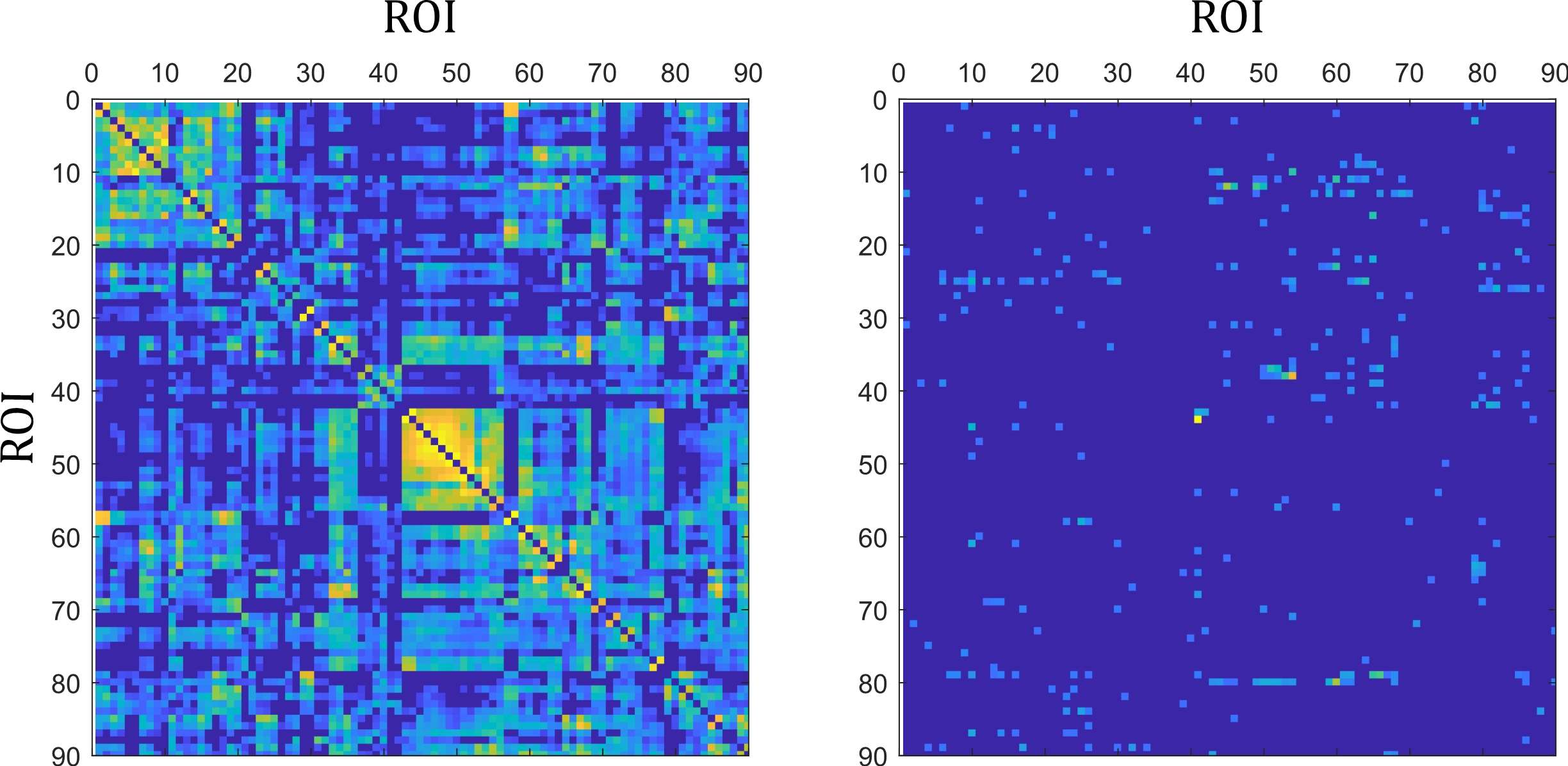
Figure 5: Qualitative comparison of brain networks generated by different methods. The left matrix is calculated by the empirical method, and the right matrix is calculated by the proposed model.

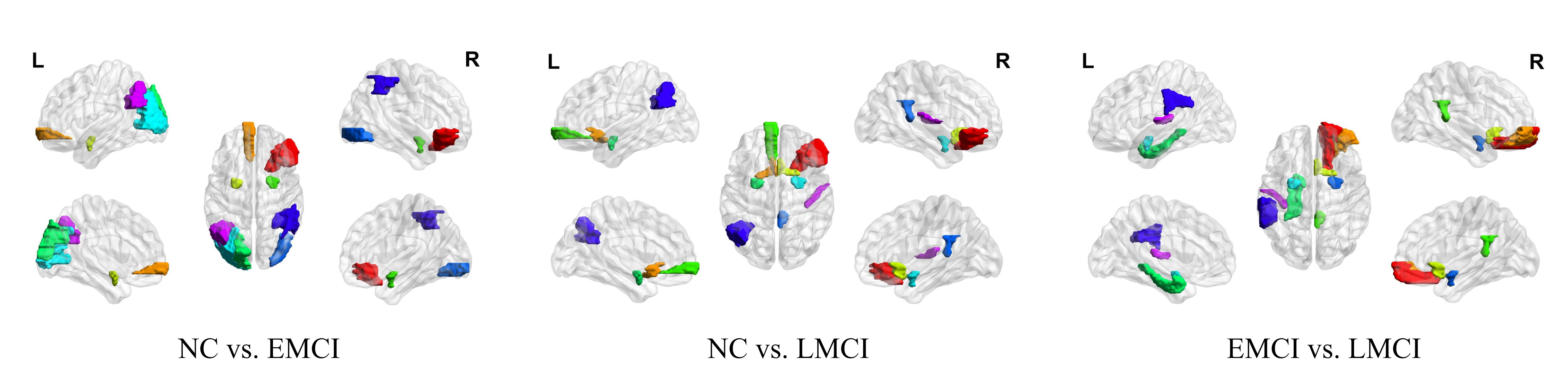
Figure 6: The spatial distribution of the top nine ROIs in three scenarios using both axial and sagittal views.

Since different brain regions have diverse impacts on the cause of MCI, in the binary classification tasks, we investigate the influence of each ROI on the accuracy prediction. It is meaningful to find MCI-related ROIs for early MCI detection and treatment. Here, we adopt the shielding method[42] to compute the important score for each ROI. The important score is calculated as one minus the mean prediction results. After sorting the important scores, we can obtain the top 10 percent ROIs for each scenario and display them using the BrainNet viewer[45]. As shown in Fig. 6, the nine important brain regions of EMCI vs. NC are: inferior frontal gyrus orbital part, superior frontal gyrus medial orbital, amygdala, superior occipital gyrus, middle occipital gyrus, inferior occipital gyrus, inferior parietal supramarginal and angular gyri, and angular gyrus. From EMCI to LMCI, the nine identified ROIs are the inferior frontal gyrus orbital part, olfactory cortex, superior frontal gyrus medial orbital, amygdala, posterior cingulate gyrus, angular gyrus, and Heschl gyrus. The important ROIs between NC and LMCI are as follows: superior frontal gyrus orbital part, middle frontal gyrus orbital part, olfactory cortex, posterior cingulate gyrus, parahippocampal gyrus, amygdala, supramarginal gyrus, and Heschl gyrus.

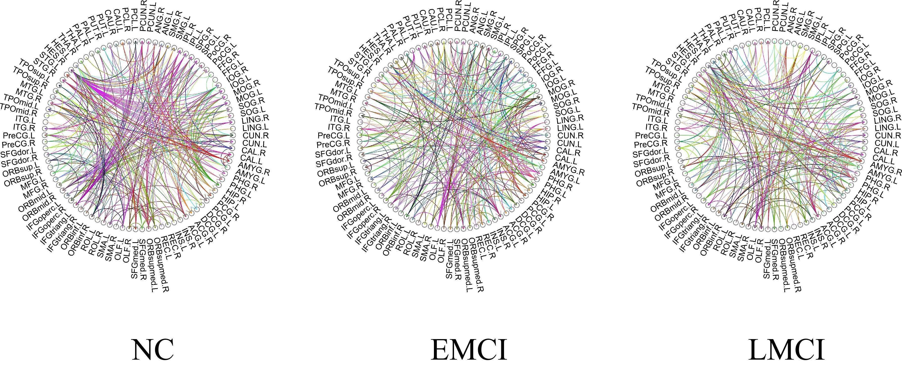
Figure 7: The generated brain effective connectivities at NC, EMCI, and LMCI, respectively. The arcs with arrows are the effective connection, and the colors have no meaning. The circles on the outside represent the brain regions.

IV-D Effective Connectivity Analysis

In addition to the fact that brain regions play an important role in disease diagnosis, the causal relationship between them can uncover the underlying pathological mechanism of MCI. In this section, we analyze the generated BECs and predict the abnormal directional connections for further study. To make the results statistically significant, we average all the BECs for each category and filter out the values that fall below the threshold of 0.1. The averaged BEC at three different stages is shown in Fig. 7 by modifying the circularGraph packages. We compute the altered effective connectivity by subtracting the averaged BEC matrix at the early stage from the later stage. As a result, a total of six altered effective connectivity matrices are obtained, consisting of the enhanced and diminished connectivities from NC to EMCI, from NC to LMCI, and from EMCI to LMCI. The altered effective connectivities are shown in Fig. 8. The top row represents the enhanced connections, and the bottom row represents the diminished connections. Each matrix is asymmetric, and the element values range from $-0.35\sim 0.35$. The positive value means the directional connection strength is enhanced, while the negative value means the directional connection strength is diminished.

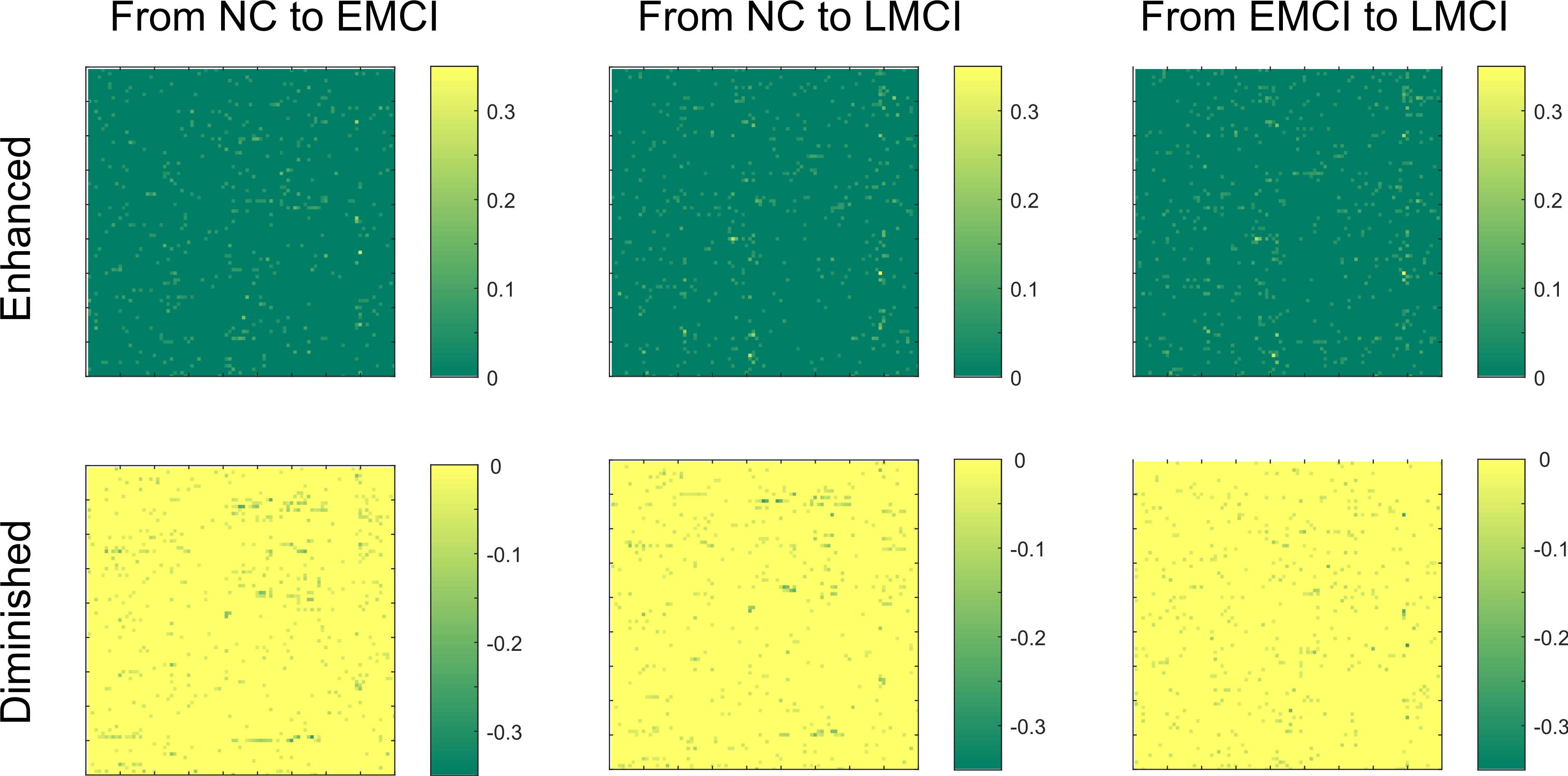
Figure 8: The altered brain effective connectivities from NC to EMCI, from NC to LMCI, and from EMCI to LMCI, respectively. The top row represents the enhanced connections, and the bottom row represents the diminished connections.

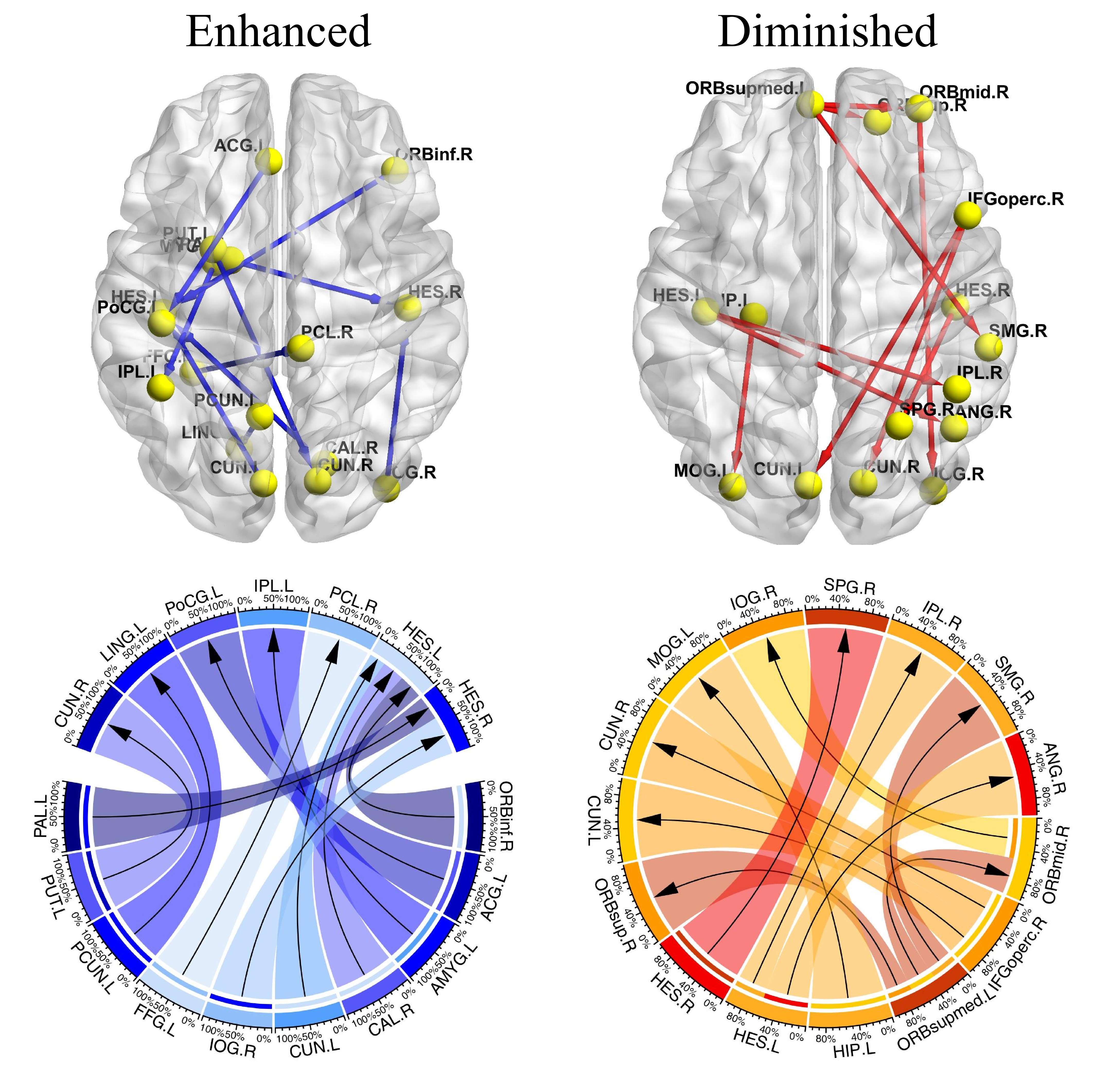
Figure 9: The top 10 enhanced and diminished effective connections from NC to EMCI.

These altered effective connections probably contribute to the cause of MCI. To find the important effective connections during the MCI progression, we sort the altered effective connections and calculate the top 10 enhanced and diminished effective connections. The results are shown in Fig. 9, Fig. 10, and Fig. 11. The enhanced and diminished connections are displayed on both the brain atlas view and the circularGraph view. From NC to EMCI, the 10 effective connections with the greatest enhancement in connection strength are ORBinf.R $\rightarrow$ HES.L, ACG.L $\rightarrow$ PoCG.L, AMYG.L $\rightarrow$ IPL.L, CAL.R $\rightarrow$ HES.L, CUN.L $\rightarrow$ HES.L, IOG.R $\rightarrow$ HES.R, FFG.L $\rightarrow$ PCL.R, PCUN.L $\rightarrow$ LING.L, PUT.L $\rightarrow$ CUN.R, PAL.L $\rightarrow$ HES.R; The 10 effective connections with the greatest diminishment in connection strength are ORBmid.R $\rightarrow$ IOG.R, IFGoperc.R $\rightarrow$ CUN.L, IFGoperc.R $\rightarrow$ CUN.R, ORBsupmed.L $\rightarrow$ ORBsup.R, ORBsupmed.L $\rightarrow$ ORBmid.R, ORBsupmed.L $\rightarrow$ SMG.R, HIP.L $\rightarrow$ MOG.L, HES.L $\rightarrow$ IPL.R, HES.L $\rightarrow$ ANG.R, HES.R $\rightarrow$ SPG.R. As the EMCI progresses to the LMCI, the top 10 enhanced effective connections are: ROL.L $\rightarrow$ AMYG.R, SMA.R $\rightarrow$ HES.L, SOG.R $\rightarrow$ PCG.R, SOG.R $\rightarrow$ HIP.L, SPG.R $\rightarrow$ HES.L, IPL.R $\rightarrow$ HES.L, THA.L $\rightarrow$ OLF.R, THA.R $\rightarrow$ AMYG.R, TPOsup.R $\rightarrow$ AMYG.L, MTG.R $\rightarrow$ AMYG.R; and the top 10 diminished effective connections are ORBinf.R $\rightarrow$ HES.L, OLF.L $\rightarrow$ SOG.R, ACG.L $\rightarrow$ PoCG.L, CAL.R $\rightarrow$ HES.L, CUN.L $\rightarrow$ HES.L, IOG.R $\rightarrow$ HES.R, FFG.L $\rightarrow$ PCL.R, FFG.R $\rightarrow$ IOG.L, PUT.L $\rightarrow$ CUN.R, PAL.L $\rightarrow$ HES.R. The enhanced effective connections between NC and LMCI groups includes ORBmid.L $\rightarrow$ TPOsup.L, ROL.L $\rightarrow$ AMYG.R, SMA.R $\rightarrow$ HES.L, SOG.R $\rightarrow$ PCG.R, SPG.R $\rightarrow$ HES.L, PAL.R $\rightarrow$ HES.L, THA.L $\rightarrow$ OLF.R, THA.R $\rightarrow$ AMYG.R, TPOsup.L $\rightarrow$ ORBmid.R, TPOsup.R $\rightarrow$ AMYG.L; and the diminished effective connections are ORBmid.R $\rightarrow$ IOG.R, IFGoperc.R $\rightarrow$ CUN.L, IFGoperc.R $\rightarrow$ CUN.R, IFGoperc.R $\rightarrow$ SOG.L, IFGoperc.R $\rightarrow$ SOG.R, ORBinf.R $\rightarrow$ ANG.L, HIP.L $\rightarrow$ MOG.L, HIP.R $\rightarrow$ IOG.R, CAL.R $\rightarrow$ AMYG.L, HES.R $\rightarrow$ SPG.R. These connection-related ROIs are consistent with the top nine important ROIs identified in the above section.

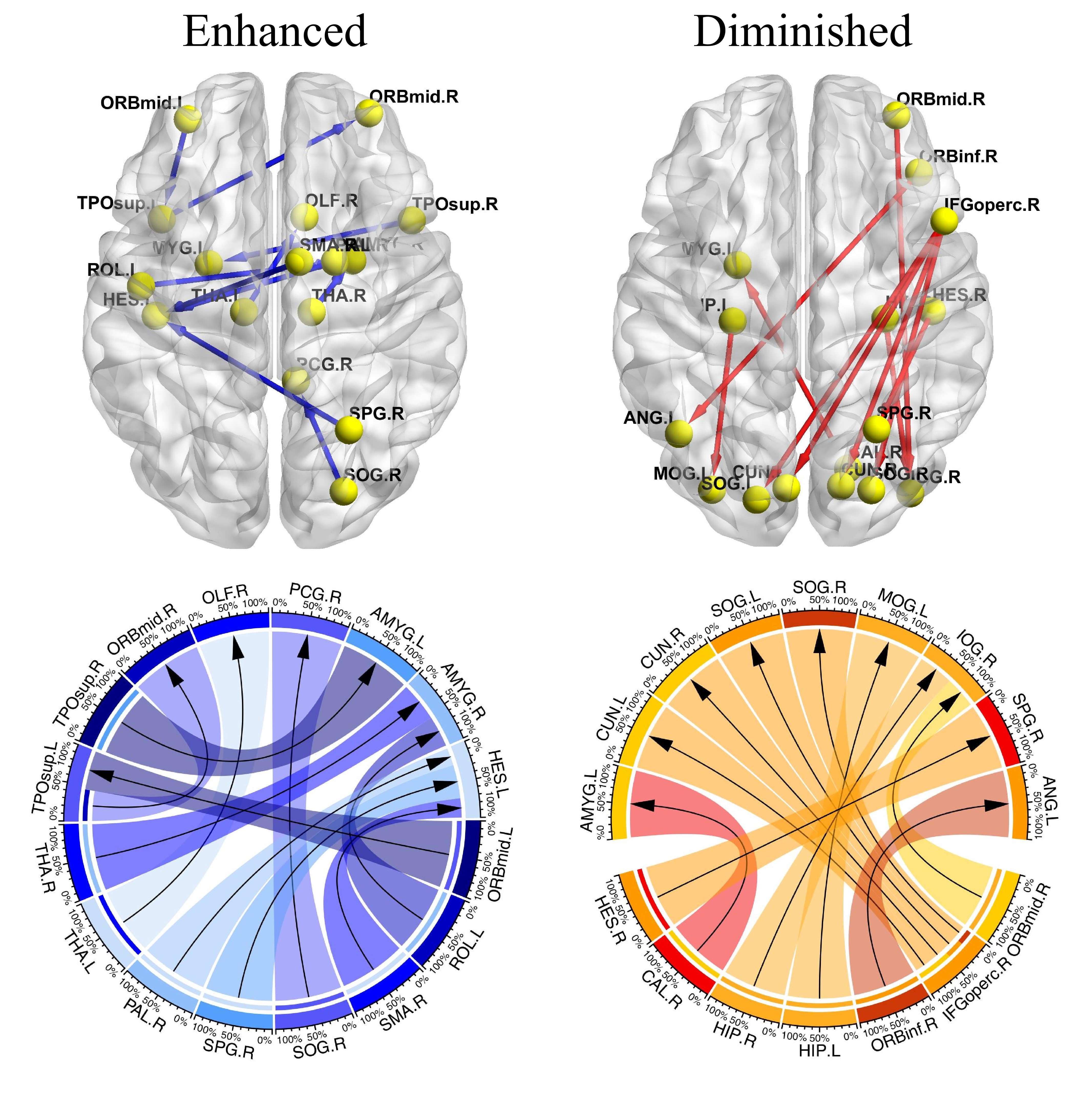
Figure 10: The top 10 enhanced and diminished effective connections from NC to LMCI.

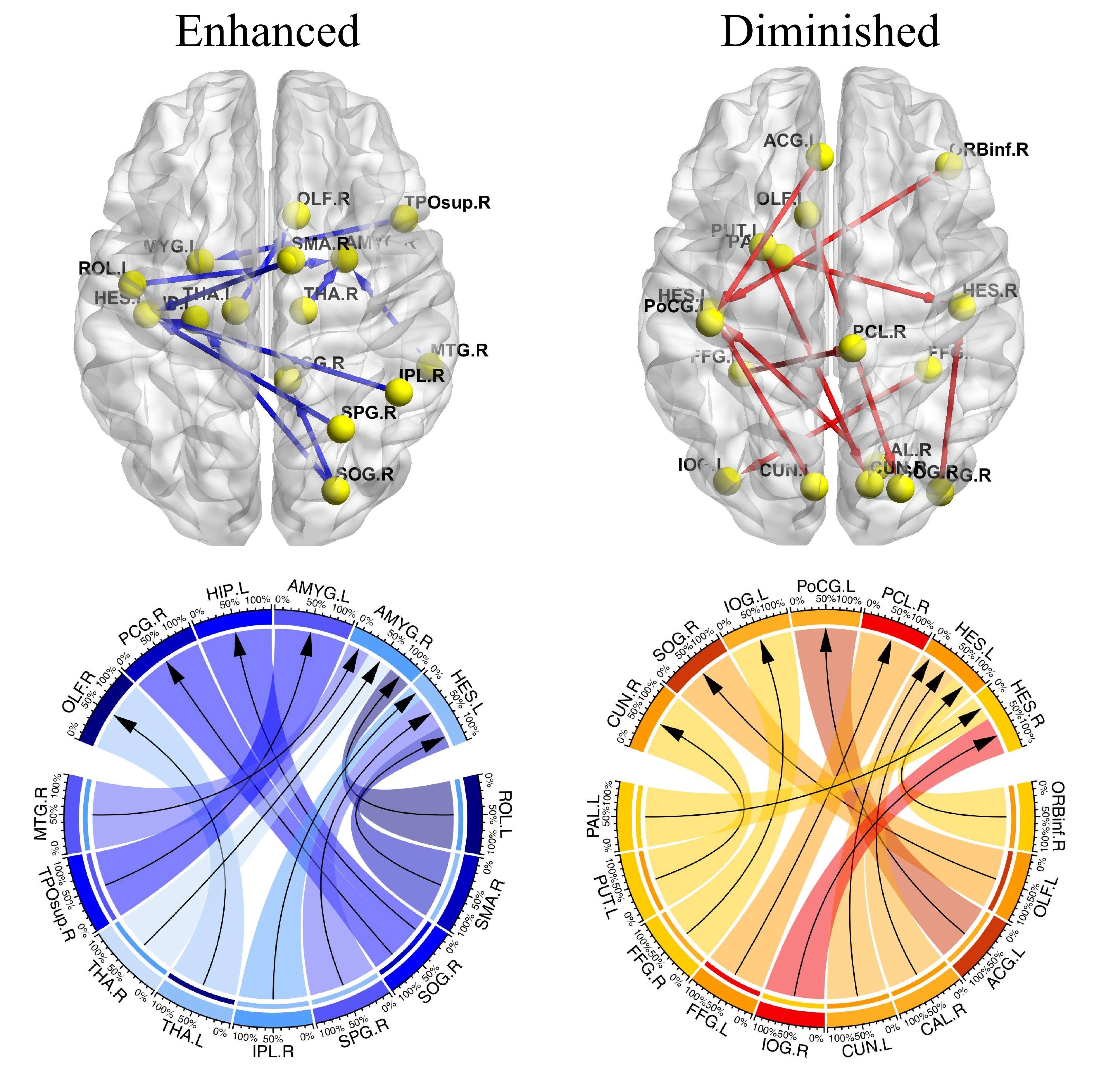
Figure 11: The top 10 enhanced and diminished effective connections from EMCI to LMCI.

IV-E Ablation Study

In our experiment, the BEC is obtained by optimizing the generator and the discriminator. To investigate whether the proposed generator and discriminator are effective, we design three variants of the proposed model and repeat ten times the 5-fold cross validations. (1) MSETD without hierarchical transformer (MSETD w/o HT). We removed the TDS and TUS, and only kept one SeTe block in the generator. (2) MSETD without SeTe blocks (MSETD w/o SeTe). In this case, we replace the SeTe with conventional 1D convolution with a kerner size of $1\times 3$. (3) MSETD without multiresolution diffusive transformer (MSETD w/o MDT). We remove the downsampling operation in the discriminator and keep the $D_{1}$. For each variant, we compute the ACCs, AUCs, SENs, and SPEs. The results are shown in Fig. 12. It can be observed that removing the hierarchical structure greatly reduces the classification performance, which shows the effectiveness and necessity of hierarchical structure for BEC generation. The SeTe block and the discriminator structure also lower the model’s classification performance to some extent. Besides, we analyze the impact of the SMA and TMA in the SeTe block. The results are displayed in Fig. 13. Both of these two modules contribute a lot to classification performance. It probably indicates that they capture the spatial and temporal characteristics that are correlated with MCI.

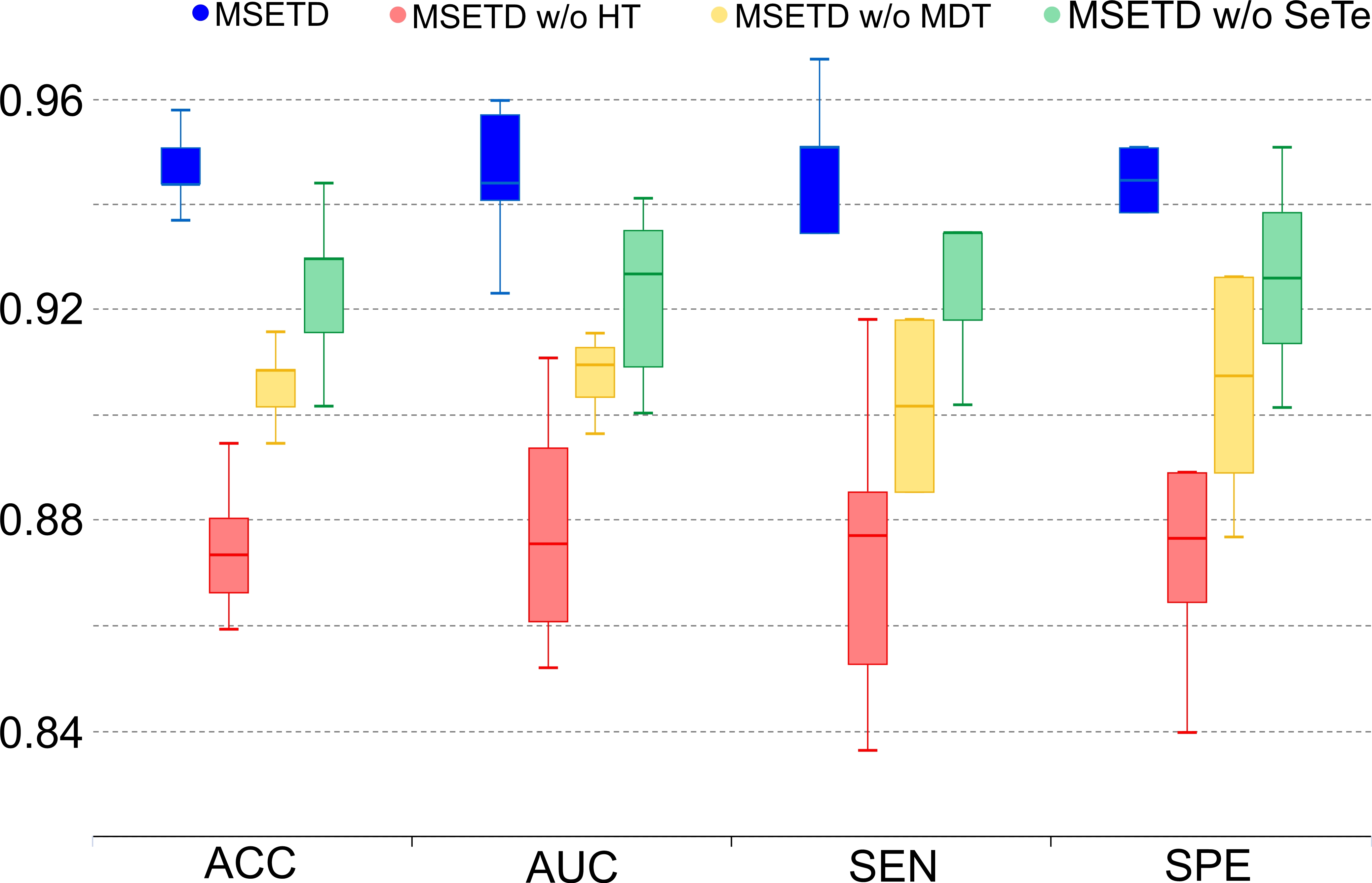
Figure 12: The impact of the proposed generator and discriminator on the model’s performance.

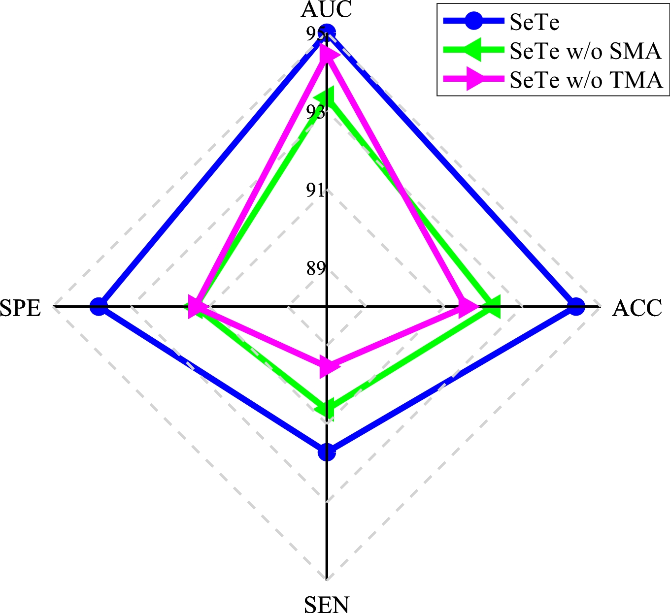
Figure 13: The influence of SeTe structure on the model’s classification performance.

Table II: The top twelve important effective connections that are highly correlated with MCI. + means enhanced connection, and - means diminished connection.

Type	Effective connection	Location
+	ORBmid.L$\rightarrow$TPOsup.L	Frontal lobe/Temporal lobe
	SOG.R$\rightarrow$PCG.R	Occipital lobe/Parietal lobe
	PAL.R$\rightarrow$HES.L	Subcortical areas/Temporal lobe
	THA.L$\rightarrow$OLF.R	Subcortical areas/Frontal lobe
	THA.R$\rightarrow$AMYG.R	Subcortical areas/Temporal lobe
	TPOsup.L$\rightarrow$ORBmid.R	Temporal lobe/Frontal lobe
-	IFGoperc.R$\rightarrow$SOG.L	Frontal lobe/Occipital lobe
	HIP.L$\rightarrow$MOG.L	Temporal lobe/Occipital lobe
	HIP.L$\rightarrow$MOG.R	Temporal lobe/Occipital lobe
	HIP.R$\rightarrow$IOG.R	Temporal lobe/Occipital lobe
	CAL.R$\rightarrow$AMYG.L	Occipital lobe/Temporal lobe
	HES.L$\rightarrow$ANG.L	Temporal lobe/Parietal lobe

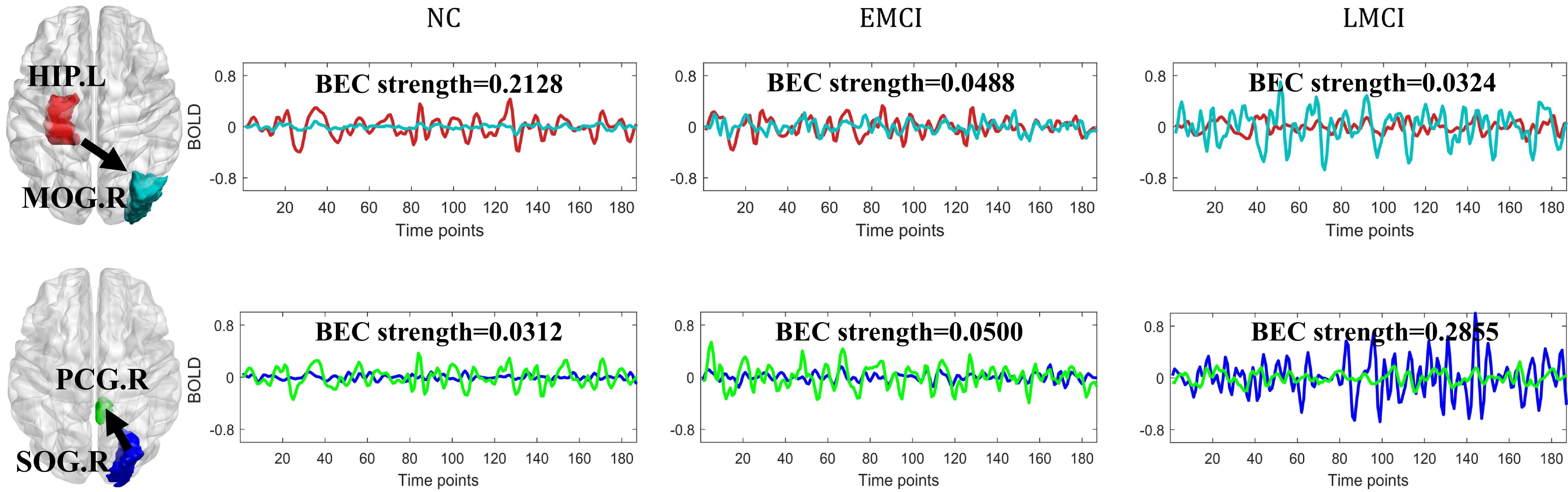
Figure 14: Visualization of ROI-based BOLD signals from two effective connections. The red arrow is the causal direction. The top row is the diminished connection, and the bottom row is the enhanced connection.

V Discussion

The proposed model can generate BEC from 4D fMRI in an end-to-end manner for MCI analysis. The ROI mask of the AAL90 atlas helps to parcellate the whole 3D volume into 90 ROIs at each time point. This operation contains many linear interpolations and ignores voxels at the boundaries of adjacent brain regions, which results in a rough ROI-based time series. To denoise the rough ROI-based time-series obtained, we employ the conditional DDPM to successively remove the noise and get a clean ROI-based time-series because of its powerful ability to generate high-quality and diverse results. As the denoising process needs thousands of steps to approach clean data, we introduce the adversarial strategy to speed the denoising process. As displayed in Fig. 12, when removing the adversarial strategy (MSETD w/o MDT), the classification performance shows a significant decrease. Also, the hierarchical structure and the SeTe block in the generator both ensure good generation results because they focus on the multi-scale spatiotemporal features and thus enhance the denoising quality.

The altered effective connections detected are important for the three scenarios. These connections are partly correlated, which is essential for discovering MCI-related biomarkers. We focus on the same altered connections between NC vs. EMCI and NC vs. LMCI. The top 12 MCI-related effective connections are shown in Table. II. The enhanced and diminished effective connection-related ROIs are identified in previous studies[46, 47, 48]. For example, the HIP has characteristics of decreasing volume and diminishing connection strength as the disease progresses[49, 50]. Also, the AMYG has been reported to process both sensory information and punishment/reward-related learning memory [51]. Disruption of AMYG-related connections can bring cognitive decline[52]. The ANG can correlate visual information with language expression. Patients with MCI lose ANG-related connections and cannot read the visual signals[53]. We display two examples for visualizing the effective connection-strength-changing process. As shown in Fig. 14, the effective connection from SOG.R to PCG.R is becoming weaker as NC progresses to LMCI. This perhaps results in the memory problem and is consistent with clinical works[54, 55]. The effective connection from HIP.L to MOG.R becomes progressively stronger during disease progression.

The proposed model still has two limitations, as follows: One is that this work ignores the causal dynamic connections between paired brain regions. The dynamic characteristics are indicative of cognitive and emotional brain activities, which play an important role in detecting the early stage of AD and understanding the pathological mechanisms. In the next work, we will explore the time delay properties of fMRI among brain regions to bridge the dynamic causal connections with biological interpretability. Another is that the input data only concentrates on the fMRI while ignoring other complementary information. Since diffusion tensor imaging (DTI) can characterize the microstructural information, it can enhance the BEC’s construction performance and make biological analyses. In the future, we will utilize the GCN and combine it with fMRI to extract complementary information for effective connectivity construction.

VI Conclusion

In this paper, we propose a multi-resolution spatiotemporal enhanced transformer denoising (MSETD) network to estimate the brain’s effective connectivity from 4-dimensional fMRI in an end-to-end manner. The denoising network is based on the conditional diffusion model, which translates noise into clean time series with blurred time series. It separates the diffusion denoising process into several successive steps and leverages the generative adversarial strategy to make the generation process more high-quality, diverse, and efficient. The spatial/temporal multi-head attention mechanisms in the generator capture the global and local connectivity features at different scales for better denoising quality improvement. The multi-resolution diffusive transformer discriminator captures the phase patterns at different scales and guides the generation process to approximate empirical samples. Results from the ADNI datasets prove the feasibility and efficiency of the proposed model. The proposed model not only achieves superior prediction performance compared with other shallow and deep-learning methods but also identifies MCI-related causal connections for better understanding pathological deterioration and discovering potential MCI biomarkers.

References

- [1] A. T. Reid, D. B. Headley, R. D. Mill, R. Sanchez-Romero, L. Q. Uddin, D. Marinazzo, D. J. Lurie, P. A. Valdés-Sosa, S. J. Hanson, B. B. Biswal et al., “Advancing functional connectivity research from association to causation,” Nature neuroscience, vol. 22, no. 11, pp. 1751–1760, 2019.
- [2] A. Avena-Koenigsberger, B. Misic, and O. Sporns, “Communication dynamics in complex brain networks,” Nature reviews neuroscience, vol. 19, no. 1, pp. 17–33, 2018.
- [3] S. Rupprechter, L. Romaniuk, P. Series, Y. Hirose, E. Hawkins, A.-L. Sandu, G. D. Waiter, C. J. McNeil, X. Shen, M. A. Harris et al., “Blunted medial prefrontal cortico-limbic reward-related effective connectivity and depression,” Brain, vol. 143, no. 6, pp. 1946–1956, 2020.
- [4] M. Mijalkov, G. Volpe, and J. B. Pereira, “Directed brain connectivity identifies widespread functional network abnormalities in parkinson’s disease,” Cerebral cortex, vol. 32, no. 3, pp. 593–607, 2022.
- [5] B. M. Hampstead, M. Khoshnoodi, W. Yan, G. Deshpande, and K. Sathian, “Patterns of effective connectivity during memory encoding and retrieval differ between patients with mild cognitive impairment and healthy older adults,” Neuroimage, vol. 124, pp. 997–1008, 2016.
- [6] S. Sami, N. Williams, L. E. Hughes, T. E. Cope, T. Rittman, I. T. Coyle-Gilchrist, R. N. Henson, and J. B. Rowe, “Neurophysiological signatures of alzheimer’s disease and frontotemporal lobar degeneration: pathology versus phenotype,” Brain, vol. 141, no. 8, pp. 2500–2510, 2018.
- [7] Y. Shi, H.-I. Suk, Y. Gao, S.-W. Lee, and D. Shen, “Leveraging coupled interaction for multimodal alzheimer’s disease diagnosis,” IEEE transactions on neural networks and learning systems, vol. 31, no. 1, pp. 186–200, 2019.
- [8] M. Scherr, L. Utz, M. Tahmasian, L. Pasquini, M. J. Grothe, J. P. Rauschecker, T. Grimmer, A. Drzezga, C. Sorg, and V. Riedl, “Effective connectivity in the default mode network is distinctively disrupted in alzheimer’s disease-a simultaneous resting-state fdg-pet/fmri study,” Human brain mapping, vol. 42, no. 13, pp. 4134–4143, 2021.
- [9] B. Ibrahim, S. Suppiah, N. Ibrahim, M. Mohamad, H. A. Hassan, N. S. Nasser, and M. I. Saripan, “Diagnostic power of resting-state fmri for detection of network connectivity in alzheimer’s disease and mild cognitive impairment: A systematic review,” Human Brain Mapping, vol. 42, no. 9, pp. 2941–2968, 2021.
- [10] W. Yin, L. Li, and F.-X. Wu, “Deep learning for brain disorder diagnosis based on fmri images,” Neurocomputing, vol. 469, pp. 332–345, 2022.
- [11] Q. Zuo, L. Lu, L. Wang, J. Zuo, and T. Ouyang, “Constructing brain functional network by adversarial temporal-spatial aligned transformer for early ad analysis,” Frontiers in Neuroscience, vol. 16, 2022.
- [12] K. J. Friston, J. Kahan, B. Biswal, and A. Razi, “A dcm for resting state fmri,” Neuroimage, vol. 94, pp. 396–407, 2014.
- [13] J. Liu, J. Ji, X. Jia, and A. Zhang, “Learning brain effective connectivity network structure using ant colony optimization combining with voxel activation information,” IEEE journal of biomedical and health informatics, vol. 24, no. 7, pp. 2028–2040, 2019.
- [14] N. Xu, R. N. Spreng, and P. C. Doerschuk, “Initial validation for the estimation of resting-state fmri effective connectivity by a generalization of the correlation approach,” Frontiers in neuroscience, vol. 11, p. 271, 2017.
- [15] A. Al-Ezzi, N. Yahya, N. Kamel, I. Faye, K. Alsaih, and E. Gunaseli, “Severity assessment of social anxiety disorder using deep learning models on brain effective connectivity,” IEEE Access, vol. 9, pp. 86 899–86 913, 2021.
- [16] S. Bagherzadeh, M. S. Shahabi, and A. Shalbaf, “Detection of schizophrenia using hybrid of deep learning and brain effective connectivity image from electroencephalogram signal,” Computers in Biology and Medicine, vol. 146, p. 105570, 2022.
- [17] J. Liu, J. Ji, G. Xun, and A. Zhang, “Inferring effective connectivity networks from fmri time series with a temporal entropy-score,” IEEE Transactions on Neural Networks and Learning Systems, vol. 33, no. 10, pp. 5993–6006, 2021.
- [18] L. Zhang, G. Huang, Z. Liang, L. Li, and Z. Zhang, “Estimating scale-free dynamic effective connectivity networks from fmri using group-wise spatial–temporal regularizations,” Neurocomputing, vol. 485, pp. 22–35, 2022.
- [19] I. Goodfellow, J. Pouget-Abadie, M. Mirza, B. Xu, D. Warde-Farley, S. Ozair, A. Courville, and Y. Bengio, “Generative adversarial networks,” Communications of the ACM, vol. 63, no. 11, pp. 139–144, 2020.
- [20] J. Ho, A. Jain, and P. Abbeel, “Denoising diffusion probabilistic models,” Advances in Neural Information Processing Systems, vol. 33, pp. 6840–6851, 2020.
- [21] Z. Dorjsembe, S. Odonchimed, and F. Xiao, “Three-dimensional medical image synthesis with denoising diffusion probabilistic models,” in Medical Imaging with Deep Learning, 2022.
- [22] Y. Xie and Q. Li, “Measurement-conditioned denoising diffusion probabilistic model for under-sampled medical image reconstruction,” in Medical Image Computing and Computer Assisted Intervention–MICCAI 2022: 25th International Conference, Singapore, September 18–22, 2022, Proceedings, Part VI. Springer, 2022, pp. 655–664.
- [23] C. Saharia, J. Ho, W. Chan, T. Salimans, D. J. Fleet, and M. Norouzi, “Image super-resolution via iterative refinement,” IEEE Transactions on Pattern Analysis and Machine Intelligence, 2022.
- [24] H.-J. Park, K. J. Friston, C. Pae, B. Park, and A. Razi, “Dynamic effective connectivity in resting state fmri,” NeuroImage, vol. 180, pp. 594–608, 2018.
- [25] A. K. Seth, “A matlab toolbox for granger causal connectivity analysis,” Journal of neuroscience methods, vol. 186, no. 2, pp. 262–273, 2010.
- [26] A. K. Seth, A. B. Barrett, and L. Barnett, “Granger causality analysis in neuroscience and neuroimaging,” Journal of Neuroscience, vol. 35, no. 8, pp. 3293–3297, 2015.
- [27] A. M. DSouza, A. Z. Abidin, L. Leistritz, and A. Wismüller, “Exploring connectivity with large-scale granger causality on resting-state functional mri,” Journal of neuroscience methods, vol. 287, pp. 68–79, 2017.
- [28] N. Talebi, A. M. Nasrabadi, I. Mohammad-Rezazadeh, and R. Coben, “Ncreann: Nonlinear causal relationship estimation by artificial neural network; applied for autism connectivity study,” IEEE transactions on medical imaging, vol. 38, no. 12, pp. 2883–2890, 2019.
- [29] Z. Abbasvandi and A. M. Nasrabadi, “A self-organized recurrent neural network for estimating the effective connectivity and its application to eeg data,” Computers in biology and medicine, vol. 110, pp. 93–107, 2019.
- [30] J. Liu, J. Ji, G. Xun, L. Yao, M. Huai, and A. Zhang, “Ec-gan: inferring brain effective connectivity via generative adversarial networks,” in Proceedings of the AAAI Conference on Artificial Intelligence, vol. 34, no. 04, 2020, pp. 4852–4859.
- [31] J. Ji, J. Liu, L. Han, and F. Wang, “Estimating effective connectivity by recurrent generative adversarial networks,” IEEE Transactions on Medical Imaging, vol. 40, no. 12, pp. 3326–3336, 2021.
- [32] A. Zou, J. Ji, M. Lei, J. Liu, and Y. Song, “Exploring brain effective connectivity networks through spatiotemporal graph convolutional models,” IEEE Transactions on Neural Networks and Learning Systems, 2022.
- [33] S. You, B. Lei, S. Wang, C. K. Chui, A. C. Cheung, Y. Liu, M. Gan, G. Wu, and Y. Shen, “Fine perceptive gans for brain mr image super-resolution in wavelet domain,” IEEE transactions on neural networks and learning systems, 2022.
- [34] S. Hu, B. Lei, S. Wang, Y. Wang, Z. Feng, and Y. Shen, “Bidirectional mapping generative adversarial networks for brain mr to pet synthesis,” IEEE Transactions on Medical Imaging, vol. 41, no. 1, pp. 145–157, 2021.
- [35] J. Hong, Y.-D. Zhang, and W. Chen, “Source-free unsupervised domain adaptation for cross-modality abdominal multi-organ segmentation,” Knowledge-Based Systems, vol. 250, p. 109155, 2022.
- [36] M. Mirza and S. Osindero, “Conditional generative adversarial nets,” arXiv preprint arXiv:1411.1784, 2014.
- [37] Y. Wang, B. Yu, L. Wang, C. Zu, D. S. Lalush, W. Lin, X. Wu, J. Zhou, D. Shen, and L. Zhou, “3d conditional generative adversarial networks for high-quality pet image estimation at low dose,” Neuroimage, vol. 174, pp. 550–562, 2018.
- [38] A. Lugmayr, M. Danelljan, A. Romero, F. Yu, R. Timofte, and L. Van Gool, “Repaint: Inpainting using denoising diffusion probabilistic models,” in Proceedings of the IEEE/CVF Conference on Computer Vision and Pattern Recognition, 2022, pp. 11 461–11 471.
- [39] N. G. Nair, K. Mei, and V. M. Patel, “At-ddpm: Restoring faces degraded by atmospheric turbulence using denoising diffusion probabilistic models,” in Proceedings of the IEEE/CVF Winter Conference on Applications of Computer Vision, 2023, pp. 3434–3443.
- [40] O. Özdenizci and R. Legenstein, “Restoring vision in adverse weather conditions with patch-based denoising diffusion models,” IEEE Transactions on Pattern Analysis and Machine Intelligence, 2023.
- [41] N. Tzourio-Mazoyer, B. Landeau, D. Papathanassiou, F. Crivello, O. Etard, N. Delcroix, B. Mazoyer, and M. Joliot, “Automated anatomical labeling of activations in spm using a macroscopic anatomical parcellation of the mni mri single-subject brain,” Neuroimage, vol. 15, no. 1, pp. 273–289, 2002.
- [42] B. Lei, Y. Zhu, S. Yu, H. Hu, Y. Xu, G. Yue, T. Wang, C. Zhao, S. Chen, P. Yang et al., “Multi-scale enhanced graph convolutional network for mild cognitive impairment detection,” Pattern Recognition, vol. 134, p. 109106, 2023.
- [43] J. Wang, X. Wang, M. Xia, X. Liao, A. Evans, and Y. He, “Gretna: a graph theoretical network analysis toolbox for imaging connectomics,” Frontiers in human neuroscience, vol. 9, p. 386, 2015.
- [44] J. Kawahara, C. J. Brown, S. P. Miller, B. G. Booth, V. Chau, R. E. Grunau, J. G. Zwicker, and G. Hamarneh, “Brainnetcnn: Convolutional neural networks for brain networks; towards predicting neurodevelopment,” NeuroImage, vol. 146, pp. 1038–1049, 2017.
- [45] M. Xia, J. Wang, and Y. He, “Brainnet viewer: a network visualization tool for human brain connectomics,” PloS one, vol. 8, no. 7, p. e68910, 2013.
- [46] S.-Y. Lin, C.-P. Lin, T.-J. Hsieh, C.-F. Lin, S.-H. Chen, Y.-P. Chao, Y.-S. Chen, C.-C. Hsu, and L.-W. Kuo, “Multiparametric graph theoretical analysis reveals altered structural and functional network topology in alzheimer’s disease,” NeuroImage: Clinical, vol. 22, p. 101680, 2019.
- [47] B. Lei, N. Cheng, A. F. Frangi, E.-L. Tan, J. Cao, P. Yang, A. Elazab, J. Du, Y. Xu, and T. Wang, “Self-calibrated brain network estimation and joint non-convex multi-task learning for identification of early alzheimer’s disease,” Medical image analysis, vol. 61, p. 101652, 2020.
- [48] B. Chen, “Abnormal cortical regions and subsystems in whole brain functional connectivity of mild cognitive impairment and alzheimer’s disease: a preliminary study,” Aging Clinical and Experimental Research, vol. 33, pp. 367–381, 2021.
- [49] N. Schuff, N. Woerner, L. Boreta, T. Kornfield, L. Shaw, J. Trojanowski, P. Thompson, C. Jack Jr, M. Weiner, and A. D. N. Initiative, “Mri of hippocampal volume loss in early alzheimer’s disease in relation to apoe genotype and biomarkers,” Brain, vol. 132, no. 4, pp. 1067–1077, 2009.
- [50] M. Tahmasian, L. Pasquini, M. Scherr, C. Meng, S. Förster, S. M. Bratec, K. Shi, I. Yakushev, M. Schwaiger, T. Grimmer et al., “The lower hippocampus global connectivity, the higher its local metabolism in alzheimer disease,” Neurology, vol. 84, no. 19, pp. 1956–1963, 2015.
- [51] T. Yang, K. Yu, X. Zhang, X. Xiao, X. Chen, Y. Fu, and B. Li, “Plastic and stimulus-specific coding of salient events in the central amygdala,” Nature, pp. 1–10, 2023.
- [52] M. Ortner, L. Pasquini, M. Barat, P. Alexopoulos, T. Grimmer, S. Förster, J. Diehl-Schmid, A. Kurz, H. Förstl, C. Zimmer et al., “Progressively disrupted intrinsic functional connectivity of basolateral amygdala in very early alzheimer’s disease,” Frontiers in neurology, vol. 7, p. 132, 2016.
- [53] E.-S. Lee, K. Yoo, Y.-B. Lee, J. Chung, J.-E. Lim, B. Yoon, and Y. Jeong, “Default mode network functional connectivity in early and late mild cognitive impairment,” Alzheimer Disease & Associated Disorders, vol. 30, no. 4, pp. 289–296, 2016.
- [54] J. Xue, H. Guo, Y. Gao, X. Wang, H. Cui, Z. Chen, B. Wang, and J. Xiang, “Altered directed functional connectivity of the hippocampus in mild cognitive impairment and alzheimer’s disease: a resting-state fmri study,” Frontiers in Aging Neuroscience, vol. 11, p. 326, 2019.
- [55] D. Berron, D. van Westen, R. Ossenkoppele, O. Strandberg, and O. Hansson, “Medial temporal lobe connectivity and its associations with cognition in early alzheimer’s disease,” Brain, vol. 143, no. 4, pp. 1233–1248, 2020.