A benchmark for computational analysis of animal behavior, using animal-borne tags

Abstract

Animal-borne sensors (‘bio-loggers’) can record a suite of kinematic and environmental data, which can elucidate animal ecophysiology and improve conservation efforts. Machine learning techniques are useful for interpreting the large amounts of data recorded by bio-loggers, but there exists no standard for comparing the different machine learning techniques in this domain. To address this, we present the Bio-logger Ethogram Benchmark (BEBE), a collection of datasets with behavioral annotations, standardized modeling tasks, and evaluation metrics. BEBE is to date the largest, most taxonomically diverse, publicly available benchmark of this type, and includes 1654 hours of data collected from 149 individuals across nine taxa. We evaluate the performance of ten different machine learning methods on BEBE, and identify key challenges to be addressed in future work. Datasets, models, and evaluation code are made publicly available at https://github.com/earthspecies/BEBE, to enable community use of BEBE as a point of comparison in methods development.

^∗ Equal contribution

^† Equal contribution

Keywords Machine Learning  $\cdot$ Bio-loggers  $\cdot$ Animal Behavior  $\cdot$ Accelerometers  $\cdot$ Time series  $\cdot$ Clustering

Animal behavior is of central interest in ecology and evolution, because an individual’s behavior helps determine its reproductive opportunities and probability of survival [16]. Additionally, understanding animal behavior can be key to identifying conservation problems and planning successful management interventions [6], for example in rearing captive animals prior to reintroduction [86], designing protected areas [80], and reducing dispersal of introduced species [82].

To study an animal’s behavior, it is useful to construct an inventory of what types of actions an individual may perform. This inventory, or ethogram, is then used to classify observed actions (Figure 1A). Using an ethogram, one can quantify, for example, the proportion of time an animal spends in different behavioral states, and how these differ between groups (e.g., sex, age, populations), or change over time (e.g., seasonally), with physiological condition (e.g., healthy vs. sick) or across different environmental contexts [4, 44].

One increasingly utilized approach for monitoring animal behavior is remote recording by animal-borne tags, or bio-loggers [71, 88]. These tags can be composed of multiple sensors such as accelerometer, gyroscope, altimeter, pressure, GPS receiver, microphone, and camera, which record time-series data on an individual’s behavior and their in situ environment. Additionally, bio-logger datasets include data from multiple many-hour tag deployments. Machine learning (ML), and in particular deep learning, is well suited for large, high complexity datasets [46], and is increasingly being used for the analysis of bio-logger data. [24, 87].

Machine learning techniques can be supervised or unsupervised. To analyze behavior, supervised learning requires bio-logger data that are manually annotated with the behaviors in an ethogram. The ML model learns from the annotated data to automatically detect and classify those behaviors in new datasets. In unsupervised learning, the ML model makes inferences about the data without relying on annotations. Unsupervised models have been employed for discovering latent behavioral patterns in bio-logger data  [47, 19, 25, 73], thereby discovering an ethogram rather than applying a pre-defined one. With supervised learning, ML could thus enable the analysis of large datasets by automating manual work, and with unsupervised learning, ML may help reveal behavioral complexity that may be otherwise hidden from human observers [66, 15].

In spite of recent interest, there is little consensus about which ML techniques are best suited to analyze bio-logger data. Studies typically test a few ML techniques on a single bio-logger dataset, e.g. [12, 13, 14, 20, 27, 28, 36, 43, 45, 56, 58, 61, 68, 73, 75, 78, 79]. Because these techniques are often adapted to the dataset at hand, it is difficult to assess how well they will generalize to other species or sensor types. Furthermore, due to differences in data collection, data pre-processing, and evaluation methods between studies, it is difficult to compare their results. This represents a missed opportunity: if there were a common framework for evaluation, then machine learning researchers could develop new techniques and compare their effectiveness with previously established ones. On the other hand, if certain techniques were shown to be well-suited for a variety of bio-logger data, then behavioral scientists could focus on applying them, rather than implementing and comparing several techniques from scratch.

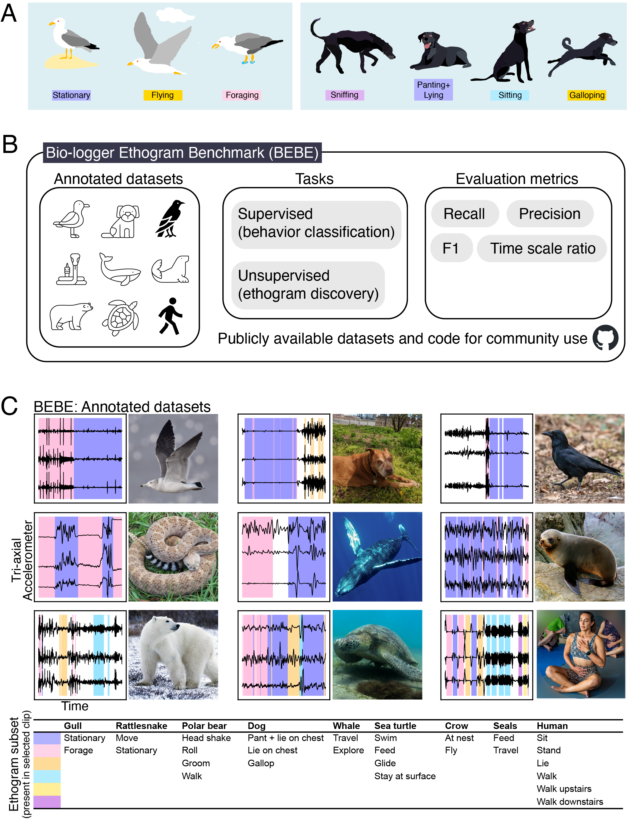
Figure 1: A) Examples of ethograms in BEBE. Left: gull ethogram with three behaviors. Right: a subset of the dog ethogram, with four behaviors. B) BEBE consists of nine annotated datasets, two tasks and a set of metrics that compare model predictions with the annotations. Datasets and code are publicly available at https://github.com/earthspecies/BEBE. C) Datasets in BEBE, with a photo of a representative individual and a 5-minute clip of annotated tri-axial accelerometer (TIA) data for each. Each accelerometer channel is min-max scaled for visualization. Top row: black-tailed gull (Larus crassirostris) [42], domestic dog (Canis familiaris) [43, 85], carrion crow (Corvus corone) [77] (see Methods). Middle row: western diamondback rattlesnake (Crotalus atrox) [20], humpback whale (Megaptera novaeangliae) [30], New Zealand fur seal (Arctocephalus forsteri) [45]. Bottom row: polar bear (Ursus maritimus) [60, 61], sea turtle (Chelonia mydas) [36], human (Homo sapiens) [3]. Table indicates annotation colors for behaviors present in these TIA recordings (for most datasets, this is a subset of the full ethogram). Gaps indicate that the behavior annotation is Unknown. For image attributions, see acknowledgments.

A commonly used tool for stimulating the development of ML techniques is the benchmark. A benchmark consists of a publicly available dataset, a problem statement specifying a model’s inputs and the desired outputs (a task), and a procedure for quantitatively evaluating a model’s success on the task (using one or several evaluation metrics). Researchers report the performance of a proposed technique on the benchmark, helping the field to draw comparisons between different techniques and consolidate knowledge about promising directions. For example, a cornerstone benchmark for image recognition is ImageNet [70], which contains over 1.2 million annotated images. For this benchmark, the task is to classify an image into one of 1000 categories, and the evaluation metric is the error rate as compared to the annotations. ImageNet has contributed to the rapid development of deep neural networks for image recognition, and deep networks have subsequently become a standard tool in many computer vision applications, including in ecology (e.g., [5, 74]).

Given their centrality in ML, benchmarks will likely be important in developing techniques for biology [83]. However, for bio-logger data analysis, previous efforts (e.g., [9, 76, 90]) have encountered obstacles to providing an adequate touchstone for model performance. For example, bio-logger datasets often are not publicly available, focus on a single species, or lack annotations for model training and/or evaluation.

In this study, we present the Bio-logger Ethogram Benchmark (BEBE), designed to capture challenges in ML-based analysis of diverse bio-logger datasets. BEBE combines nine datasets collected by various research groups, each with behavioral annotations, as well as two tasks with evaluation metrics (Figure 1B). These datasets are diverse, spanning multiple species, individuals, behavioral states, sampling rates, and sensor types (Figure 1C), as well as large in size, ranging from six to over a thousand hours in duration. BEBE comprises body motion data collected using tri-axial accelerometers (TIA) and gyroscopes, as well as pressure and conductivity data from environmental sensors. We define tasks and evaluation metrics for both supervised and unsupervised ML. The supervised task (behavior classification) is to predict an animal’s behavioral state based on recorded motions and, where available, environmental data. The unsupervised task (ethogram discovery) is to cluster the data such that each cluster can be given a behavioral interpretation. For both tasks, we evaluate a model’s performance by comparison with the annotations.

As a baseline for future work, we tested a number of previously proposed methods on BEBE. These methods include classical ML, such as random forests and hidden Markov models, as well as deep neural networks. We present the current best techniques on BEBE and identify challenges posed by these datasets.

Going forward, we intend BEBE to be a tool that the bio-logger and machine learning communities can use to test newly proposed modeling approaches. Ultimately, we expect BEBE will spur innovations that improve performance. To this end, all datasets, models, and evaluation code presented in this work are available at https://github.com/earthspecies/BEBE for community use.

Given that BEBE is aimed at methodological development, we are also seeking contributions to create an expanded benchmark with improved taxonomic coverage, a broader range of sensor types, additional standardization, and a wider variety of modeling tasks. Details about how to contribute in this way can also be found at our website.

1 Results

1.1 Benchmark Datasets

We brought together nine animal motion datasets into a benchmark collection called the Bio-logger Ethogram Benchmark (BEBE) (Table 1). These data were all collected in previous studies. Of the datasets included in BEBE, four are publicly available for the first time (Whale, Crow, Rattlesnake, Gull) and five were already publicly available (HAR, Polar bear, Sea turtle, Dog).

In each dataset, data were recorded by bio-loggers attached to several different individuals of the given species. Each dataset contains one species, except for the Seal dataset which contains four Otariid species. These bio-loggers collected kinematic and environmental time series data, such as acceleration, angular velocity, pressure, and conductivity. While each dataset in BEBE includes acceleration data, different hardware configurations were used across studies. As a result, each dataset comes with its own particular set of data channels, and with its own sampling rate.

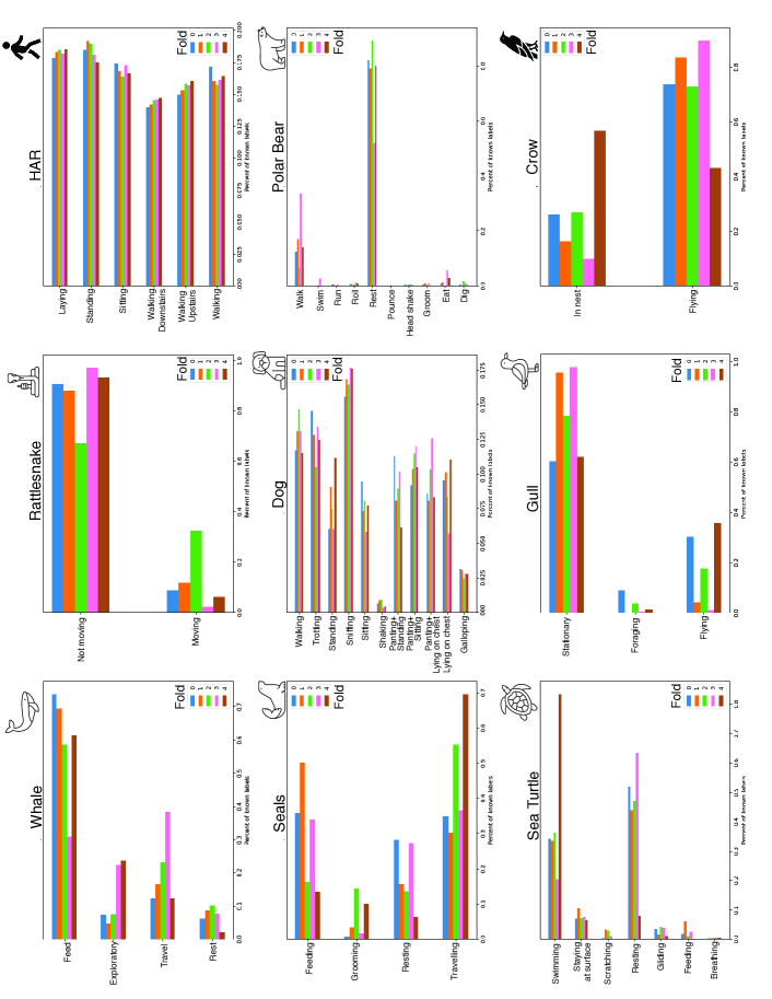
Figure S1: Representation of each behavioral class in the BEBE datasets. The bars represent the proportion of sampled time steps with the given annotation, as a fraction of the total time steps with a known behavioral annotation in that fold. All behavioral classes for each dataset are listed.

Table 1: Summary of datasets in BEBE. Out of nine datasets, one comes from humans, three come from other terrestrial species, three come from aquatic species, and two come from flying species. For a full list of behavioral classes and their representation across folds, see Figure S1. Datasets marked with an asterisk are publicly available for the first time in BEBE. The final column indicates the type of data that was used to make the behavioral annotations.

Dataset name License	Species	Tag Attach. Pos.	$\#$ ind.	$\#$ beh. classes	Example beh. classes	Sample rate (Hz)	Data channels	Dur. (hrs)	Annot. Dur. (hrs)	Mean Annot. Dur. (sec.)	Annot. method
HAR [3, 69] Custom	Humans	Waist	30	6	Sitting, Standing, Walking	50	TIA, gyroscope	6.2	4.2	17.5	Direct Obs.
Rattlesnake∗ [20] Creative Commons	Western diamondback rattlesnake	Body	13	2	Moving, Not Moving	1	TIA	31.0	31.0	710.7	Direct Obs.
Polar Bear [60, 61] Public Domain	Polar bear	Neck	5	10	Pouncing, Swimming, Eating	16	TIA, conductivity	1108.4	196.1	127.2	Video
Dog [43, 85] Creative Commons	Domestic dog	Back and Neck	45	11	Galloping, Sniffing, Sitting	100	2x TIA, 2x gyroscope	29.5	16.9	15.5	Video
Whale∗ [30] TBD	Humpback whale	Dorsal Surface or Flank	8	4	Traveling, Feeding, Exploratory (dive types)	5	TIA, depth, speed	184.6	114.1	119.8	Motion
Sea Turtle [36] Public Domain	Green turtle	Carapace	14	7	Swimming, Scratching, Gliding	20	TIA, gyroscope, depth	77.1	67.8	47.2	Video
Seal [45] Creative Commons	Otariid spp.	Back	12	4	Traveling, Foraging, Resting	25	TIA, depth	14.0	11.6	24.8	Video
Gull∗ [42] Creative Commons	Black-tailed gull	Back or Abdomen	11	3	Flying, Stationary, Foraging	25	TIA	88.7	85.0	2823.7	Video
Crow∗ (see Methods) Creative Commons	Carrion crow	Tail	11	2	Flying, In Nest	50	TIA	114.6	3.4	14.1	Audio

In addition to the time series bio-logger data, each dataset in BEBE comes with human-generated behavioral annotations. In each dataset, each sampled time step is annotated with the current behavioral state of the tagged individual, which can be one of several discrete behavioral classes. At some time steps, it was not possible to observe the individual, or it was not possible to classify the individual’s behavior using the predefined behavioral classes. In these cases, this time step is annotated as Unknown. We describe below how we account for these Unknown behavioral annotations during model training and evaluation (also see Methods).

There are multiple time scales of behavior represented across the nine ethograms in BEBE, with some datasets including brief activities (e.g. shaking), and some including longer duration activities (e.g. foraging). In Table 1 we report the mean duration of an annotation in each dataset, as a rough estimate of the mean duration an individual spends in a given behavioral state.

We split each dataset into five groups, or folds, so that no individual appears in more than one fold. During cross validation, we train a model on the individuals from four folds, and test it on the individuals from the remaining fold. For all datasets, Figure S1 shows the proportion of behavior classes for each fold.

1.2 Formulation of Tasks and Evaluation

We propose two tasks and corresponding evaluation schemes, one for supervised ML and one for unsupervised ML. For both tasks, model performance is evaluated by comparison with the behavioral annotations, although the specifics differ (see below). The training and evaluation pipelines for these tasks are summarized in Figure 2A. The entire pipeline, including training, inference, and evaluation, is repeated for each dataset in BEBE.

Supervised Task

The supervised task (top row in Figure 2A; example in Figure 2B) reflects the use of ML for automatic behavior classification. The researcher has defined the ethogram categories of interest and annotated the dataset. The annotated train set is used to train an ML model that can predict behavior from time-series input. During inference, the trained model predicts behaviors for the test set. The evaluation of the supervised task is straightforward, as the behavioral predictions on the test set (made during inference) can be directly compared with the annotations.

Unsupervised task

The unsupervised task (bottom row in Figure 2A; example in Figure 2C) reflects the use of ML in ethogram discovery. The model is only trained with time-series data recorded from bio-loggers, without the use of annotations. The model learns to partition the data in the train set into clusters that optimize some objective (e.g., minimize variance within clusters). During inference, the trained model partitions time-series data based on its learned parameters (e.g., cluster centroids). Here, evaluation is more challenging: how can we quantitatively assess whether the unsupervised model has discovered an appropriate clustering of the data, when it may find a different partition than the human annotators? We propose a contingency analysis similar to the overclustering used by [38] (see Figure 2D for details), which determines a mapping between the discovered clusters and annotations. Using this mapping, a model’s clustering performance can be assigned scores in analogy with the supervised case.

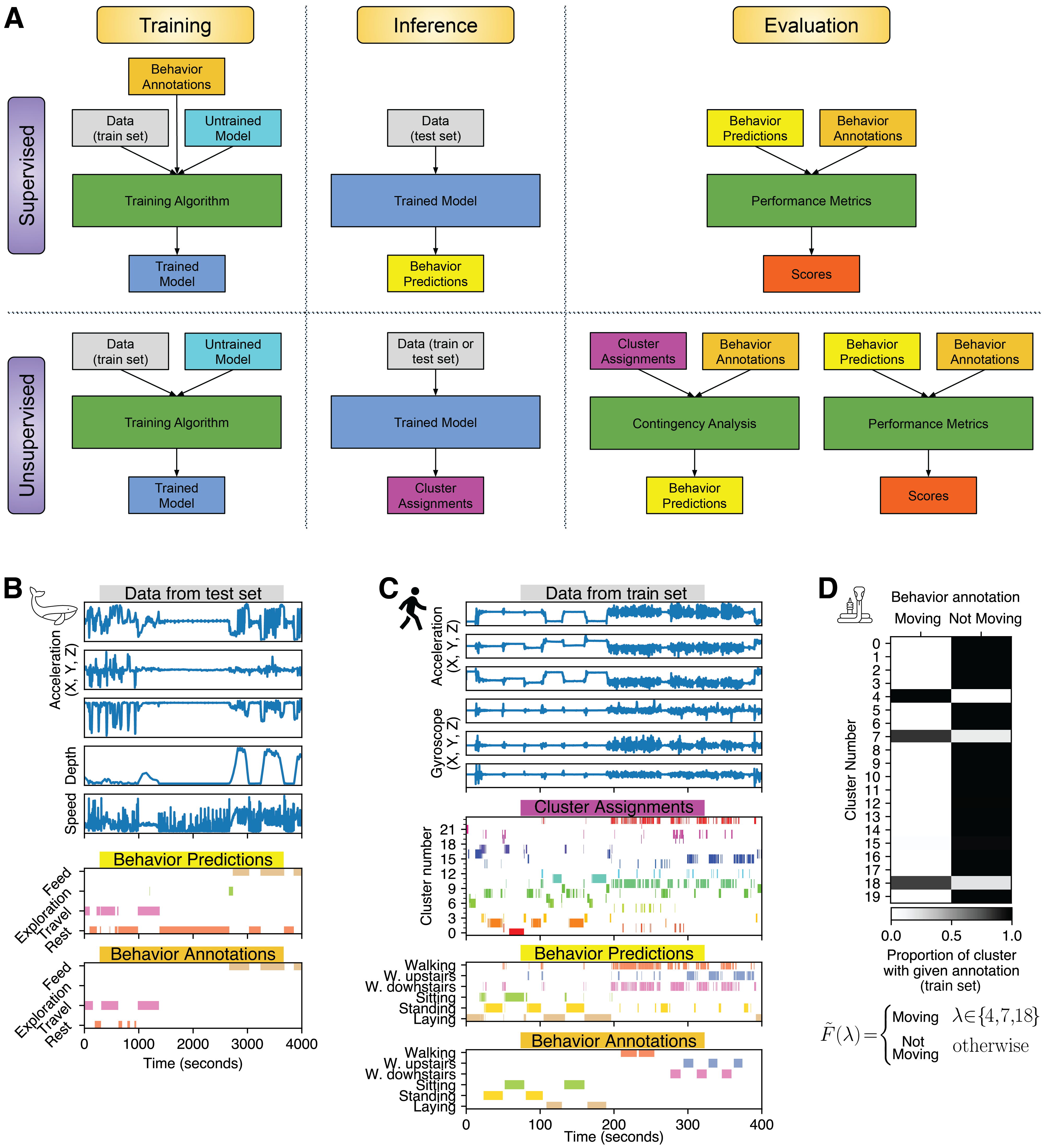
Figure 2: A) Summary of training and evaluation. For both supervised and unsupervised models, we divide our process into three steps. In the first step, the model learns from the train set of one dataset. In the supervised case, this includes behavioral annotations. In the second step, the model makes predictions about the behavioral annotation (supervised) or cluster (unsupervised) of each sampled time step. In the third step, the model’s predictions are evaluated based on their agreement with known behavioral annotations. In the unsupervised case, an extra contingency analysis is required. B) Analysis of a supervised model’s predictions, using example data from the Whale dataset [30], and predictions made by a convolutional recurrent neural network (CRNN) model. The trained model is fed raw time series data, which it uses to make behavior predictions. These predictions are compared with annotations to arrive at performance scores. In this case, the model predicts the annotations well. Gaps in the behavior annotations indicate the behavior is Unknown at those samples; those samples are ignored in the evaluation metrics. (Caption continued on next page)

(Figure 2 continued) C) Analysis of an unsupervised model’s predictions, using example data from the train set of the human (HAR) dataset [3], and predictions made by a hidden Markov model. The trained model is fed raw time series data, which it assigns to clusters. The contingency analysis is applied to the cluster assignments in order to obtain behavior predictions. These predictions are compared with annotations to arrive at performance scores. In this example, the model does not always successfully separate Sitting and Standing into different clusters: the second sitting interval in the behavior annotations (green bar) corresponds to standing (yellow bar) instead of Sitting in the behavior predictions. D) Contingency analysis, based on data from the Rattlesnake dataset [20] and using cluster assignments created using our implementation of the MotionMapper [8] model. We form a contingency matrix (top) based on the train set, which quantifies how well each of the two behavioral classes are represented in each cluster. We see that clusters 4, 7, and 18 have more samples which are annotated with Moving than which are annotated with Not Moving. Then, we define the contingency mapping $\tilde{F}$ by assigning, to each cluster index, the behavioral class which is best represented in that cluster (bottom): all samples in clusters 4, 7, and 18 will get mapped to a behavior prediction of Moving, whereas samples in all other clusters will be mapped to Not Moving. $\tilde{F}$ can then be used on cluster assignments predicted for the train and test set to obtain behavior predictions for all samples.

Evaluation metrics

Models are evaluated on their ability to predict behavior annotations. For each individual, we measure classification precision, recall, and F1 scores averaged across all sampled time steps from that individual and averaged across all behavioral classes (see Methods). We disregard the time steps for which the annotation is Unknown.

To characterize how well a model’s predictions reflect the time scale of behaviors, we introduce a metric called the time scale ratio (TSR) that evaluates a model’s recovery of the mean annotation duration (listed in Table 1). Specifically, TSR equals $\ln(\frac{\textrm{Mean predicted duration}}{\textrm{Mean annotation duration}})$, so a value of zero is optimal. A negative TSR indicates that the model over-segments the time-series data (i.e. predicts unrealistically rapid transitions between behavioral states), whereas a positive TSR indicates that the model under-segments the data (i.e. predicts unrealistically slow transitions between behavioral states). The TSR is a coarse metric that should only be taken as an indicator of situations where a model dramatically over- or under-segments the data (see Methods).

1.3 Baseline Models

As a baseline for future work, we trained and evaluated a number of supervised and unsupervised models (Table 2) on our proposed tasks.

Table 2: Models investigated. For implementation details, see Methods.

Model Name	Super- vised?	Description	Previous Application Examples
CNN	Yes	A convolutional neural network, consisting of two one-dimensional convolutional layers and a linear prediction head.	[10, 23]
CRNN	Yes	A convolutional-recurrent neural network, consisting of two one-dimensional convolutional layers, a gated recurrent unit, and a linear prediction head.	[59]
RF	Yes	Random forests classifier using 100 decision trees. Makes predictions based on hand-chosen summary statistics.	Reviewed in [81, 87]
$k$-means	No	$k$-means clustering is applied to sampled time steps $x_{t}$.	[73]
Wavelet $k$-means	No	Morlet wavelet transform is applied to each data channel. $k$-means clustering is applied to transformed data.	[73]
GMM	No	Gaussian mixture model with $N$ components is applied to sampled time steps $x_{t}$.	[13]
HMM	No	Unsupervised hidden Markov model with Gaussian observations.	[47, 89]
Motion- Mapper	No	Morlet wavelet transform is applied to each data channel. Transformed data are reduced to two dimensions using UMAP [57], and then clustered using watershed transform.	[8]
VAME	No	An autoencoder neural network structured as a sequence of gated recurrent units. After training, $k$-means clustering is applied to the learned latent representation of the data.	[53]
IIC	No	A convolutional neural network with per-frame invariant information clustering [38] objective. The network was structured as four one-dimensional convolutional layers and a linear prediction head.	[54]
Random	No	As a baseline, each sampled time step is randomly assigned to a cluster with uniform probability	None

We trained and evaluated our models using a cross validation procedure. Most models have a set of hyperparameters (e.g., learning rate) which must be selected before training. For each model and each dataset, we performed an initial grid search to select hyperparameters, using the first fold of the dataset as the test set. We saved the hyperparameters that led to the highest test F1 score, and used these hyperparameters for training using the remaining train/test splits. The reported scores are averaged across individuals taken from these four train/test splits.

A common technique in analysis of acceleration data is to isolate acceleration due to gravity using a low pass filter [76], resulting in separate static and dynamic acceleration channels. It has been shown that the choice of low pass cutoff frequency can have a strong effect on subsequent analyses [50]. Often, this frequency is chosen based on expert knowledge of an individual’s physiology and typical movement patterns. As an alternative data-driven approach, we treated the low pass cutoff frequency as a hyperparameter to be selected during model training (see Methods).

1.4 Model Performance Results

Supervised task

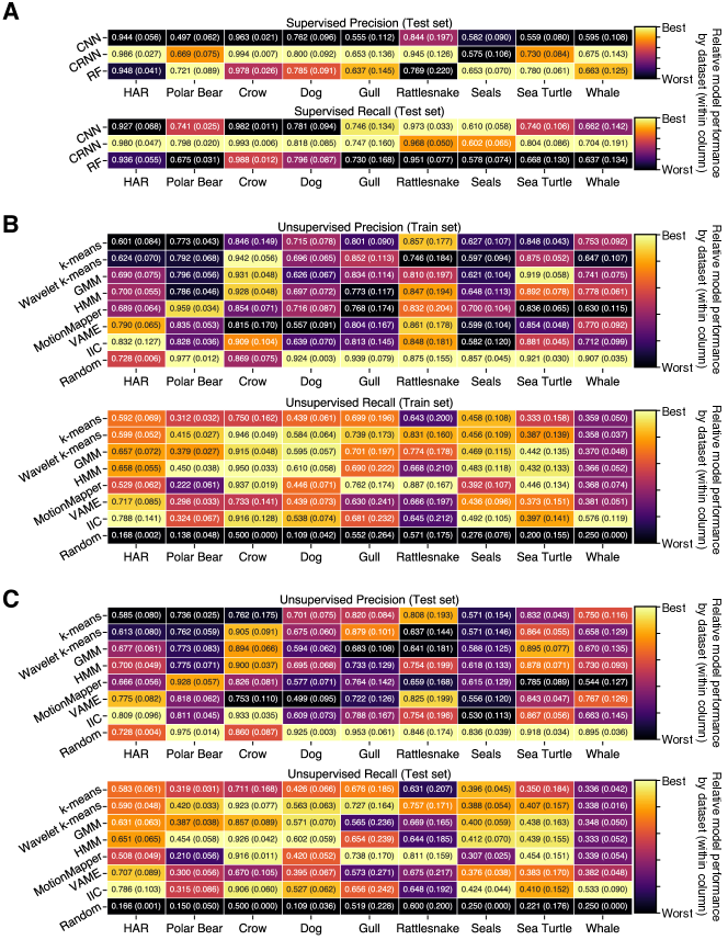
Figure S2: Model results on precision and recall for supervised and unsupervised tasks, across all datasets in BEBE. Each table is color-coded such that within a dataset (column), the brightest color indicates the best performing model for that metric, and the darkest color indicates the worst performing model. Numbers indicate the average score across individuals in a data subset (train or test) of the four folds not used for hyperparameter optimization, with the standard deviation in parentheses. A) Supervised task on test sets. B) Unsupervised task on train sets. C) Unsupervised task on test sets.

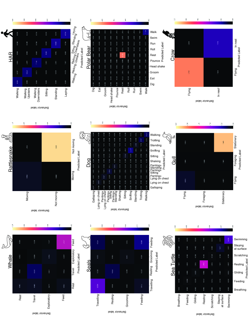
Figure S3: Confusion matrices for CRNN predictions versus behavioral labels, for all nine datasets in BEBE. Numbers represent the fraction of total labeled data. Computed for data taken from the test sets of the four cross validation steps that were not used for hyperparameter selection. Confusion matrices for the other models can be found on the Zenodo data repository.

F1 and TSR scores for the supervised task are presented in Figure 3A. Precision and recall scores (Figure S2A) and example confusion matrices (Figure S3) are presented in the Supplemental Information. We focus on the relative performance of models within a dataset, because the complex differences between the nine datasets in BEBE (e.g., between species) hinder comparisons. In terms of classification performance, the CRNN model performed the best, achieving the best F1 on eight datasets and the best recall scores on seven datasets in BEBE. The TSR scores of CRNN were better than CNN and RF on seven out of nine datasets. Therefore, CRNN sets a strong baseline for future developments in supervised behavior classification, in terms of both its classification performance and its ability to capture realistic time scales of behavior.

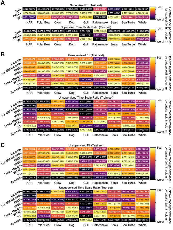
Figure 3: Model results on F1 and Time Scale Ratio for supervised and unsupervised tasks, across all datasets in BEBE. Each table is color-coded such that within a dataset (column), the brightest color indicates the best performing model for that metric, and the darkest color indicates the worst performing model. Numbers indicate the average score across individuals in a subset (train or test) of the four folds not used for hyperparameter optimization, with the standard deviation in parentheses. A) Supervised task on test sets. Out of nine datasets, CRNN does best on eight datasets for F1 and seven datasets for the Time Scale Ratio, as indicated by the bright yellow entries in its row. B) Unsupervised task on train sets. In contrast to the supervised task, there is no clear best model overall. IIC does best on three datasets for F1 and three datasets for Time Scale Ratio, while HMM does best on three datasets for F1. C) Unsupervised task on test sets. The general pattern of results is the same as for the unsupervised task on the train sets, with no clear best model overall. IIC does best on three datasets for F1 and two for Time Scale Ratio, while HMM does best for three datasets for F1 and two datasets for Time Scale Ratio. For precision and recall results, see Figure S2.

Unsupervised task

F1 and TSR scores on the unsupervised task are presented in Figures 3B-C, with precision and recall scores in the Supplemental Information (Figure S2).

There are multiple datasets where several models perform similarly well in terms of F1 score (e.g. many models achieve F1$\approx 0.9$ on the Crow dataset). Yet there is consistently a large difference between the performance of the best and worst models. On average across datasets, the difference between the mean test F1 of the best and worst performing models (excluding Random) is 0.24, with the smallest difference on the Sea Turtle dataset (0.087) and the largest difference on the HAR dataset (0.33).

Unlike in the supervised case, it is not possible to identify a single type of model which performs clearly better than the rest. In terms of F1 score on the train and test data, IIC and HMM each outperform other models on three out of nine datasets. HMM and IIC also both perform well in terms of TSR on both train and test data, relative to other models.

Of the other models, Wavelet $k$-means and GMM often have similar F1 score to HMM. However, GMM tends to have more negative TSR score, which indicates that it tends to over-segment the data more than HMM. MotionMapper had high variance in its relative performance; while it achieved competitive F1 and TSR scores on some datasets (e.g. Rattlesnake, Sea Turtle), it had lower performance on several other datasets. Finally, $k$-means and VAME consistently had lower F1 performance than other models, and $k$-means additionally performed poorly on TSR.

Looking across the nine datasets used in BEBE, the dataset used for evaluation has a strong effect on the relative performance of different model types. However, due to the large number of confounding variables, it is not clear how one would predict which types of datasets favor which types of models. It is clear that evaluating models on multiple datasets, as we have done, is vital to ensure generalizable conclusions about relative model performance.

Supervised versus unsupervised task

Overall, performance on the unsupervised task was below that of the supervised task. On average, the F1 score on the test set of the best supervised model surpassed the best unsupervised model by 0.19. Given the current performance of models, behavioral annotations remain valuable for ML analysis of bio-logger data, as they enable training of the more effective supervised methods. They also enable evaluation for specific datasets, which is especially important given the variability of performance across datasets.

Common versus rare behavioral states

To examine how model performance relates to class imbalance, we plotted F1 scores of the CRNN models we tested as a function of the amount of training data in each class (Figure 4). As one would expect, we find that CRNN models are, on average, better able to identify behaviors that are represented in a large proportion of the training data, or in a large overall number of training datapoints (e.g., Resting, Flying). For behavioral classes with low representation in the training data, we found that the models struggled to identify behaviors such as foraging and scratching. The signature of these behaviors in the recorded motion data may be relatively subtle. In contrast, even with relatively little training data, models performed well at identifying behaviors with strong motion characteristics such as Shaking, Galloping, or Moving.

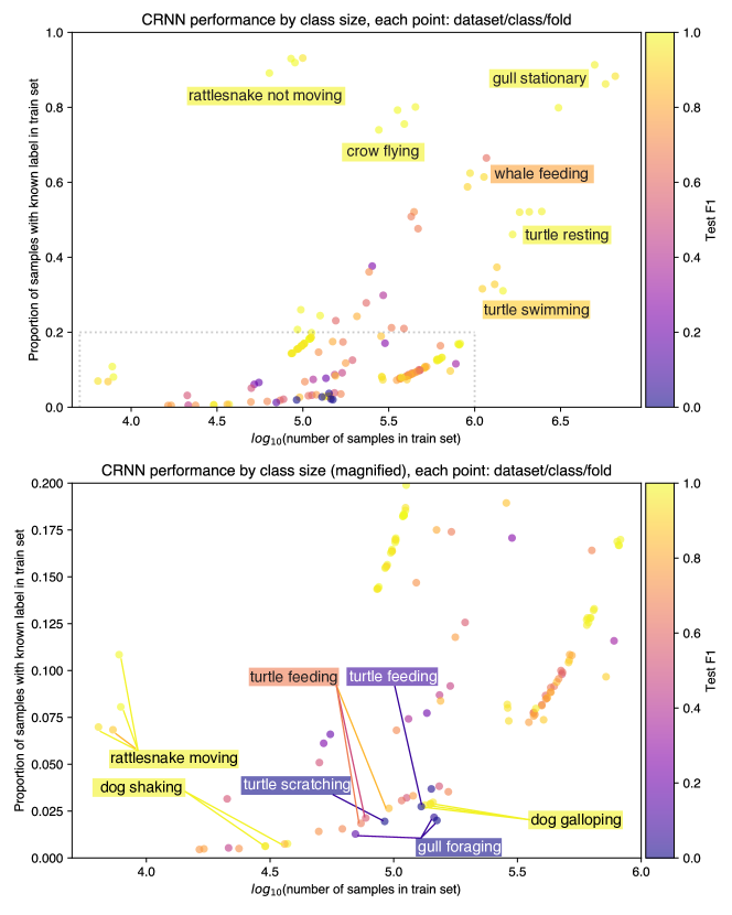
Figure 4: F1 scores vary with the representation of behavioral classes in the train set, as shown in CRNN models’ performance. Each point represents the test F1 score for one behavioral class, in one dataset, for one train/test split of a fold in that dataset. Brighter colors indicate better performance. The horizontal axis represents the number of datapoints of a given class in the train set, and the vertical axis represents the proportion of datapoints in a given class, as a fraction of the total datapoints in the train set with a known behavioral annotation. Behaviors with high proportion and and a large number of train set datapoints are readily classified (top panel). But only some behaviors with a relatively small proportion or number of datapoints in the train set can be classified (bottom panel).

Inter-dataset comparisons

Given the complex differences between datasets, it is not clear how to predict how a model would perform on one dataset, based on its performance on another dataset in BEBE. For example, one might expect similar performance on the Gull and Crow datasets as they are the two flying species in BEBE. However, this is not the case, possibly due to differences in tag placement, calibration procedure, sampling rate, annotation method, and behavior classes used. As ML methods are applied to datasets outside of BEBE, we expect that it will continue to be difficult to predict how well a given type of model will perform on a given dataset.

Static and dynamic acceleration

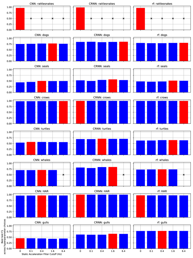
Figure S4: Hyperparameter optimization of static acceleration cutoff frequency (supervised models). Y-axis indicates the best F1 score on the test set of the fold used for hyperparameter optimization, chosen from all hyperparameter with the same cutoff frequency. A cross marker indicates that this dataset/model pair did not test hyperparameters for the cutoff. The hyperparameter chosen was not consistent within a dataset. Most models do not show large performance variation based on this hyperparameter.

As a hyperparameter, we varied the cutoff frequency used to separate static from dynamic acceleration. Reviewing the top F1 score for each cutoff frequency, model type, and dataset, we found that the cutoff frequency selected during the hyperparameter tuning procedure was not consistent within a dataset (Figures S4-S5). IIC was sensitive to this choice of hyperparameter across several datasets, whereas most types of models (e.g. all supervised models) were not. We additionally found that, in some cases, the selected cutoff was at a higher frequency (6.4 Hz) than what might be recommended based on body size [50]. Therefore, it is unclear how and when these types of data manipulations will influence model performance.

Computational limitations

On the majority of datasets in BEBE, the classification performance of RF approached that of CRNN. Additionally, RF is computationally cheaper to train and apply to new data, because it typically has fewer parameters than CRNN (or CNN), and does not rely on GPU acceleration. Therefore, a random forests model may be adequate in some applications, especially in the face of limited computational resources. Similarly, in the unsupervised setting, it may be preferable to choose a model such as HMM, which has good performance on many datasets in BEBE, but does not rely on GPU acceleration for training.

1.5 Challenges presented by BEBE

We outline four challenging aspects of the tasks presented in BEBE, which we believe will be particularly important to consider during future model development.

Individual variation

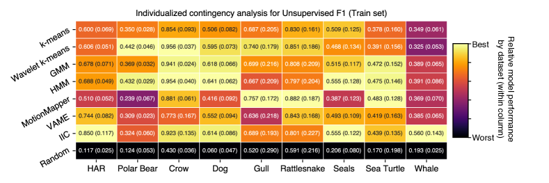
Figure S7: Individualized contingency analysis. To quantify how individual variation affects model performance, we re-evaluated unsupervised model predictions on the train set using a different method of contingency analysis than Equation 3. Rather than performing contingency analysis using the entire train set, we perform contingency analysis separately for each individual in the train set. More precisely, for each individual $i$, we assume there exists a function $F_{i}\colon\{0,\dots,N-1\}\to\{c_{1},\dots,c_{C}\}$ which assigns each cluster to its behavioral class, and that these $F_{i}$ can vary between individuals. Then, for each individual $i$ we calculate an estimate $\tilde{F}_{i}$ of $F_{i}$ by setting, for each $\lambda\in\{0,\dots,N-1\},$ $\tilde{F}_{i}(\lambda)=\operatorname{argmax}_{c\in\{c_{1},\dots,c_{C}\}}\Big{|}\{x_{t}\mid l_{t}=c\text{ and }\lambda_{t}=\lambda\text{ and }x_{t}\text{ is sampled from individual }i\}\Big{|}.$ In this table we report Individualized F1 scores, using this individualized contingency analysis, instead of previously described contingency analysis (Equation 3). When we allow clusters to be assigned to different behaviors for different individuals, performance improves for all models, with an average improvement of 0.074 across models and datasets (excluding Random). The largest improvements are observed for the Rattlesnake dataset.

There is variation in motion between individuals, and according to sensor placement on individuals’ bodies [32]. We found that these random effects are difficult for models to account for. For both supervised and unsupervised models, the average difference in the F1 score between the best and worst individual in each test set was 0.16. For additional analysis of how individual variation affects performance, see Figure S7.

Multimodality

Most datasets in BEBE also include data channels other than acceleration. In both supervised and unsupervised settings, a key design choice is how to fuse data coming from different modalities [31].

Because these data channels each come with their own units of measurement, this additionally presents a problem for unsupervised models that use Euclidean distance to measure similarity. In particular, this is a problem for the $k$-means, Wavelet $k$-means, MotionMapper, and VAME models we tested. In all these situations, we normalized the data before computing Euclidean distance (see Methods). However, better methods for accounting for differences in units likely exist. For example, GMM and HMM both use maximum likelihood estimates to predict cluster assignments.

Time scales

Behavior occurs at different time scales [1, 7]. For the supervised task, the dominance of CRNN across datasets demonstrates the importance of incorporating time scale as a learnable parameter (in contrast to RF and CNN where it is fixed). We observed a related trend for the unsupervised models, where models that only consider single timepoints (e.g., $k$-means, GMM) perform worse on the TSR compared to models that incorporate temporal context (e.g., HMM, IIC). As ML techniques are applied to other datasets, we expect the best performance will come from models that can automatically adapt the time scale of their analyses to the data. Alternatively, one could jointly model behaviors that occur at different time scales, as in Hierarchical Hidden Markov Models [29, 26, 1].

Class imbalance

Most of the datasets in BEBE contain behavioral classes which are poorly represented in the recorded data (Figure 4, Figure S1). Recall and F1 of these poorly represented classes may be improved by adjusting training objectives [48]. In the unsupervised setting, improvements may be possible through dataset-specific feature engineering. For example, in a swimming animal, discovery of behaviors which occur near the water surface may be facilitated by nonlinearly rescaling pressure sensor data.

2 Discussion

To support the development of ML methods for behavior classification and ethogram discovery, we designed the Bio-logger Ethogram Benchmark (BEBE), a collection of nine annotated bio-logger datasets and two tasks with evaluation metrics. BEBE is the largest, most diverse, publicly available bio-logger benchmark to date. We implemented baseline models for the supervised and unsupervised task to serve as a point of comparison for future methods. Out of the supervised models we tested, the convolutional-recurrent neural network was best able to classify behaviors, while simultaneously capturing the typical time scale of these behaviors. We also showed that no single model dominates at the unsupervised task across all datasets in BEBE. However, hidden Markov models and neural networks trained with an invariant information clustering objective each provide a competitive baseline on a subset of datasets. Overall, our results suggest that there is much potential for applications in monitoring animal behavior with ML, as well as opportunity for innovation in ML-based ethogram analysis of bio-logger time-series.

To use BEBE as a benchmark, researchers should use the code at https://github.com/earthspecies/BEBE, which provides standardized templates for users to implement, train, and evaluate a new type of model on the datasets in BEBE. This repository also contains code to train a model presented in this work on a new dataset.

Evaluation metrics

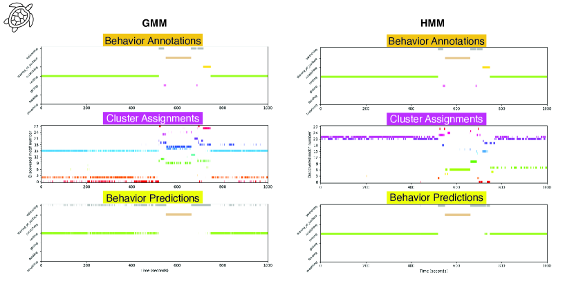
Figure S6: Unsupervised model predictions for the same test data from the Sea Turtle dataset. Top row of panels depict the ground truth behavior annotations (same for both models). Middle row depicts the cluster assignments for each model, and the bottom row depicts the behavior predictions after the contingency analysis. Overall, GMM (left) and HMM (right) achieved similar F1 scores of .406 and .397, respectively. However, GMM had TSR of -3.04 versus CRNN with TSR of -1.260. These TSR scores indicate that, while both models tend to over-segment the data, GMM does so to a much greater degree. In the figure, the GMM predicts rapid switching between two behavioral states (resting and swimming), whereas the HMM does not predict this type of switching. Therefore, in this case TSR helps distinguish predictions which are more realistic (HMM) from those that are less so (GMM).

A benchmark’s evaluation metrics should align with a field’s goals and real-world requirements, such that benchmark progress is a meaningful proxy for progress in methods development [64, 67]. BEBE utilizes previously published datasets reflecting a variety of scientific applications, and was designed in collaboration between ML researchers and behavioral ecologists. We introduced two evaluation methods that are not widely used. The first, TSR, is designed to reflect how well a model predicts the typical time scale of behavior. We found that TSR was useful for determining when a model tended to highly over-segment data (e.g. Figure S6).

The second evaluation method introduced is the contingency analysis, which provides a framework for comparing the quality of clusters produced by ethogram discovery models. For the purpose of model evaluation, this method assigns a behavioral class to each discovered cluster based on their co-occurrence. Because contingency analysis is applied to model predictions before computing performance scores, the details of how these assignments are performed may have a strong influence on relative model rankings. As better ethogram discovery methods are developed, this influence may be worthy of further investigation.

Potential limitations

Benchmarks may direct excessive focus toward finding a single system that improves evaluation metrics, at the expense of qualitative assessments of performance. This may discourage fields from pursuing a variety of methods which can be adapted to different study systems [18]. For this reason, BEBE reports evaluation metrics for each datasets, rather than averaging [67]. We caution against over-optimizing TSR because it is only a coarse indicator of the duration of behavioral states; for example, annotators may under-sample or ignore brief changes in behavioral state, leading to low TSR.

Several research groups contributed datasets to BEBE, so there is variation in the annotation schemes. While some variation is desirable in order to promote generalizable methods development, it also hinders between-dataset comparisons. These types of comparisons could illuminate how a model’s predictive ability is related to biological factors, such as phylogeny or body size, and to non-biological factors, such as dataset size or choice of ethogram. This limitation could be addressed by increasing the number of datasets available in BEBE and by better data standardization. Data annotation methods may also be reflected in model performance. For datasets where annotation was based on visual observation of the animal, some behaviors may be difficult to distinguish based on motion data alone. This may cap potential model performance below its ideal maximum by an unknown amount. Finally, some annotation error is likely present in the datasets in BEBE. Errors in annotations may affect estimates of model performance, in ways that are difficult to detect and thus to account for.

Model development

Promising avenues to improve performance include: (1) improved model design, including transformers [84]; (2) data augmentations; (3) transfer learning, (i.e. analyzing species-specific bio-logger data using models pre-trained on larger, less specific bio-logger datasets); and (4) expert-led data pre-processing and feature selection. Methods that do not use machine learning, such as rule-based classifiers designed by experts [76], would provide an additional baseline for model performance. We encourage others to publish improvements on our baseline results.

Benchmark development

Bio-loggers can shed new light on conservation problems and interventions, as well as on patterns of animal behavior [35, 40, 83]. In BEBE, we propose two general-purpose tasks for behavior prediction and discovery. Other analyses could be useful, such as detecting unusual patterns in data [62] that may indicate changes in behavior or environmental conditions [37], or counting the rate at which a specific type of behavioral event occurs [4]. A future benchmark could formalize tasks and evaluation metrics for use-cases that arise in these settings.

We expect that BEBE will also be of use to those developing on-device ML [42]. A future benchmark could explore additional evaluation metrics to promote advances in on-device ML [42], such as device energy consumption metrics to assess on-device feasibility. This could additionally give insight into environmental impacts due to model usage [33, 67, 83].

BEBE focuses on body motion and environmental sensors. However, we believe that similar public benchmarking efforts will be vital as ML is used to process large amounts of video, audio, and movement data recorded using bio-loggers [81]. A future benchmark could include data types not examined in BEBE.

Call for Collaboration

The code repository includes instructions on how datasets outside of BEBE may be formatted for use with the methods in BEBE. Interested researchers may make their formatted datasets discoverable from the BEBE repository. Such datasets would not become part of BEBE, which must remain standardized.

However, it is typical for benchmarks to be updated when key challenges are sufficiently met [18]. In light of the preceding discussion, we seek community contributions that could lead to a more comprehensive benchmark, with three main objectives:

1. To provide researchers with evidence to choose the best modeling framework for their study system,

2. To enable analyses which compare recorded behavior across taxa, and

3. To formalize tasks which reflect a variety of real-world applications, including conservation applications.

We expect these objectives will be best served by a benchmark with more diversity in its representation of taxa, data types, tag placement positions, sensor configurations, ethograms, and modeling tasks. Possible contributions include (1) annotated datasets to be made openly available to the research community (whether already available or not), (2) design of data and annotation standardization, and (3) design of benchmark tasks that reflect applications of ML and bio-logger technology. For any ensuing publications, contributors would have the option to co-author the manuscript. Interested researchers should follow the instructions at https://github.com/earthspecies/BEBE.

We have proposed that benchmarks can encourage the development and rigorous evaluation of ML methods for behavioral ecology. We envision many possible future outcomes for this line of research: for example, best practices for bio-logger data analysis, an ML-based toolkit that can be adapted to different study systems, or powerful species-agnostic tools that can be applied across taxa and sensor types. In the future, ML could allow for fast and reliable interpretation of bio-logger data, and could reveal previously unknown behavioral complexity in large and complex bio-logger datasets, especially for taxa for which direct observation is near impossible. These could, in turn, inform more effective conservation interventions, as well as guide the development and testing of hypotheses about animal behavior.

3 Methods

Datasets in BEBE

Dataset collection

A dataset had to meet the following criteria to be included in BEBE:

1. Include fine-scale animal motion data;

2. Include annotations of animal behavioral states;

3. Comprise data recorded from tags attached to at least five individuals in order to reflect variation in sensor placement and individual motion patterns,;

4. Contain over 100000 sampled time steps with behavioral annotations;

5. Contribute to a diversity of taxa, as well as a balance among the categories of terrestrial, aquatic, and aerial species

6. Be licensed for modification and redistribution; or come with permission from dataset authors for modification and public distribution.

Four datasets were not previously publicly available and were collected by coauthors (Whale: A. Friedlaender; Crow: D. Canestrari, V. Baglione, V. Moreno-González, C. Rutz, E. Trapote; Gull: T. Maekawa, K. Yoda; Rattlesnake: D. DeSantis, V. Mata-Silva). For these datasets, coauthors provided permission to publicly distribute the data. The Crow dataset was not previously published and therefore we describe it in more detail below. Through an informal literature search, we found five publicly available datasets (Human, Polar Bear, Dog, Sea Turtle, Seal). Of these, four were collected by coauthors (Dog: O. Vainio, A. Vehkaoja; Sea Turtle: L. Jeantet, D. Chevallier; Seal: M. Ladds) and one was in the public domain (Polar Bear: A. Pagano). Finally, we assessed datasets from papers covered by a recent systematic literature review of automatic behavioral classification from bio-loggers [81]. [81] provides a table with the results of their systematic review, containing metadata on whether a paper used supervised learning, species, number of individuals, and number of timepoints. We looked exclusively at the supervised learning papers because these would require annotated datasets (criterion 2). Assessing criteria 1, 3, and 4 above resulted in twelve potential datasets out of 214. Of the twelve, two were already included in BEBE (Rattlesnake, Sea Turtle), nine studied terrestrial animals, a category which was already well-represented in BEBE, and one did not provide annotations. Therefore, no new datasets were added based on the results of the systematic literature review by [81].

Tag design and data collection in carrion crows

The data logger, called miniDTAG, was adapted from a 2.6-g bat tag integrating microphone, tri-axial accelerometer and tri-axial magnetometer [77] with changes that enable long duration recordings on medium-sized birds. The triaxial accelerometer (Kionix KX022-1020 configured for ± 8 g full scale, 16-bit resolution) was sampled at 1000 Hz and decimated to a sampling rate of 200 Hz before saving to a 32 GB flash memory. The 1.2 Ah lithium primary battery (Saft LS14250) allowed continuous recording for about 6 days both in lab and field settings. Each miniDTAG was packaged with a micro radio transmitter (Biotrack Picopip Ag376) and attached to the two central tail feathers with a piece of the stem of a coloured balloon following the procedure described in [72]. The thin rubber balloon material progressively deteriorated and finally broke, letting the miniDTAG falling to the ground, where it was radio-tracked using a Sika Biotrack receiver.

Accelerometer data were calibrated using Matlab tools from www.soundtags.org following standard procedures [39, 55]. The sensor channel was decimated by a factor of 4 before calibration, thus fitting sampling rates of 50 Hz. Calibration performance was assessed by visually inspecting the estimated field intensity of the accelerometer.

For the present study, we tagged 11 individuals (5 males and 6 females), from 7 different territories. Data were collected in spring 2019, when all the birds were raising their nestlings. The miniDTAG plus battery (12.5g) accounted on average (± SE) for the 2.66 ± 0.09% of the crow body mass (range 2.29 – 3.15%). None of the crows abandoned the territory or deserted the nest after being tagged. From the recordings of these individuals, we selected 20 clips for annotation, favoring clips where begging vocalizations and wing beats could be identified at multiple times during the recording (see Annotations below).

Dataset Annotation and Preprocessing Details

For full implementation details, we refer the reader to the dataset preprocessing source code. For two datasets (Sea Turtle, Gull), the average magnitude of the acceleration vector varied by more than 10% between tag deployments. To control for these differences, we normalized the tri-axial acceleration channels so that the average magnitude of the acceleration vector was equal to 1. We do not perform any additional special pre-processing steps on the datasets in BEBE, and we left each dataset in its original measurement units (but see model specific processing below).

Annotations

In all datasets in BEBE, the annotations reflect individuals’ behavioral states, as opposed to behavioral events [4]. In other words, all annotations indicated time intervals when a behavior occurred, rather than the rate of discrete behavioral events. The modeling tasks and evaluation procedures are designed with this in mind. With the exception of one dataset (Crow), the annotations in BEBE are derived from annotations made in the original studies. As a result, datasets in BEBE are annotated in a variety of ways, and in some cases are annotated with a small number of behavioral classes (Figure S1).

For the Crow dataset, we windowed the recorded data into 5-second long non-overlapping clips. Each accelerometer clip came with synchronized audio, which we used to assign behavioral annotations. If there were sounds of wingbeats or soaring for the entire duration of a clip, we annotated all sampled time steps in that clip as Flying. Similarly, if a clip included sounds of chick begging calls, we annotated all sampled time steps in that clip as In Nest. For the remaining eight datasets, we used annotations as provided by original dataset authors. For behaviors with few annotations, we treat these behaviors as Unknown (see dataset preprocessing source code for details).

For the Polar Bear dataset, we manually synchronized the published annotations and recorded time series data based on occurrence of head shakes, which have a brief and characteristic acceleration signature. This step was performed, but not documented, in the original publication.

Time Scales

Animal behavior can be described hierarchically, in which actions are nested into multiple time scales [1, 7]: for example, the human behavior Walking may be hierarchically composed of two repeating, shorter time-scale behaviors, the left and right forward steps. For simplicity, in this study we focus on a single non-hierarchical set of annotations per dataset. However, there are multiple time scales represented across the nine ethograms in BEBE. For example, some datasets reflect brief, low-level activities (e.g. shaking, moving), whereas some reflect longer, higher-level activities (e.g. foraging, exploration). In order to give a rough quantification of the time scales present in these ethograms, for each dataset we computed the average amount of time an individual spends in a known behavioral state, before it switches to a different known behavioral state or an Unknown state. This quantity is reported in Table 1 as the mean annotation duration. The mean annotation duration should only be taken as a rough estimate of the typical duration of a behavioral state, because the annotations in the original studies were not necessarily produced with the intention of measuring onsets and offsets of behavioral states.

For the Polar Bear dataset, to compute mean annotation duration, we had to account for the fact that the video footage used to make annotations was duty cycled. Because of this duty cycling, there are periodic intervals of up to 90 seconds in which annotations are Unknown. To account for these Unknown intervals, we assumed that if the bear is in the same behavioral state before and after an Unknown interval of less than 91 seconds, then the bear was in that behavioral state during the Unknown interval. This procedure was only used to compute mean annotation duration, and not to add additional annotations for model training or evaluation.

Dataset Splits

A key part of a benchmark dataset is how it partitions the data used for model training (the train set) from the data used for model evaluation (the test set). This evaluation provides an estimate of how well a model performs outside of its train set (generalization). Therefore, the specific partition chosen determines what domains the ML model should generalize over.

In BEBE, we split each dataset into five groups (folds), which are used in a cross validation procedure. During cross validation, each time the model is trained, the train set consists of the data from four of these five folds, and the test set consists of the data from the remaining fold. For each dataset in BEBE, we divided the data so that no individual appears in more than one fold, and so that each fold has the same number of individuals represented ($\pm 1$ individual). Therefore, during testing, a model’s performance reflects its ability to generalize to new individuals, where effects such as tag placement [32] may influence model predictions.

Figure S1 displays the distribution of annotations across folds for all datasets in BEBE. Most datasets in BEBE have some behaviors with high representation, and some behaviors with very low representation.

Time Series Data and Annotations

Each dataset consists of a collection of multivariate discrete time series, where each time series $\{x_{t}\}_{t\in\{1,2,\dots,T\}}$ consists of samples $x_{t}\in\mathbb{R}^{D}$. Here $D$ is the number of data channels and $T$ is the number of sampled time steps. Note that the number $T$ may vary between different time series contained in a single dataset. Each time series is sampled from one bio-logger deployment attached to one individual, and is sampled continuously at a fixed dataset-specific sampling rate.

Each time series in a dataset also comes with a sequence of annotations $\{l_{t}\}_{t\in\{1,2,\dots,T\}}$, where each $l_{t}\in\{\textit{Unknown},c_{1},c_{2},\dots,c_{C}\}$ encodes either the behavioral class $c_{j}$ of the animal at time $t$, or the fact that the behavioral class is Unknown. Here $C$ denotes the number of known behavioral classes in the dataset. The behavioral classes $c_{j}$ vary between datasets in BEBE, and could be e.g. $c_{j}=\textit{Foraging},c_{j}=\textit{Sniffing},$ or $c_{j}=\textit{Flying}.$

3.0.1 Supervised task

Task Description

For supervised models, the task is to predict the behavioral annotation $l_{t}$ of each sampled time step $x_{t}$ (Figure 2B). During training, models are given access to the behavioral annotations in the train set. We refer the reader to [81, 87] for reviews of studies with a similar task description.

Evaluation Metrics: Classification

Trained models are evaluated on their ability to predict the behavioral annotations of the test set. For each individual in the test set, we measure classification precision, recall and F1 scores averaged across all sampled time steps from that individual and averaged across all behavioral classes. In measuring these scores, we disregard the model’s predictions for those time steps $x_{t}$ for which $l_{t}=\textit{Unknown}$. More precisely, for each individual in the test set we measure:

$$\operatorname{Prec}=\frac{1}{C}\sum_{j=1}^{C}\operatorname{Prec}_{j},\quad\operatorname{Rec}=\frac{1}{C}\sum_{j=1}^{C}\operatorname{Rec}_{j},\quad\operatorname{F1}=\frac{1}{C}\sum_{j=1}^{C}\operatorname{F1}_{j},$$ (1)

where for each behavioral class index $j\in\{1,\dots,C\},$

$$\operatorname{Prec}_{j}=\frac{\operatorname{TP}_{j}}{\operatorname{TP}_{j}+\operatorname{FP}_{j}},\quad\operatorname{Rec}_{j}=\frac{\operatorname{TP}_{j}}{\operatorname{TP}_{j}+\operatorname{FN}_{j}},\quad\operatorname{F1}_{j}=2\cdot\frac{\operatorname{Prec}_{j}\cdot\operatorname{Rec}_{j}}{\operatorname{Prec}_{j}+\operatorname{Rec}_{j}}.$$

Here, $\operatorname{TP}_{j},\operatorname{FP}_{j},$ and $\operatorname{FN}_{j}$ denote, respectively, the number of sampled time steps correctly predicted to be of class $c_{j}$ (true positives), the number incorrectly predicted to be of class $c_{j}$ (false positives), and the number incorrectly predicted to be not of class $c_{j}$ (false negatives). Precision, recall, and F1 range between 0 and 1, with 1 reflecting optimal performance. After computing these scores for each individual, we calculate the average taken across all individuals in the test set.

For a behavioral class $c$, the recall score measures the proportion of timepoints in $c$ that also were predicted correctly to be $c$. Therefore, for a single behavioral class, recall can be perfect (equal 1) if the model predicts all timepoints to be $c$. On the other hand, precision measures the proportion of correct predictions among all timepoints predicted to be $c$. Therefore, for a single behavioral class, precision can be perfect (equal 1) if the model predicts no timepoints to be $c$. The F1 score combines precision and recall with equal weighting, by taking the harmonic mean of the two scores.

We do not use prediction accuracy, as this measure is highly influenced by annotation imbalance. For example, in the Rattlesnake test set [20], 92 percent of the sampled time steps have the annotation $l_{t}=\textit{Not Moving}$. A model whose output is $\tilde{l}_{t}=\textit{Not Moving}$ for all $x_{t}$ will have accuracy of $.92$. While this is close to the optimum of $1$, it reflects no real predictive ability of the model.

Taking inspiration from human speech recognition [52], we considered including additional evaluation metrics. For example, we experimented with metrics intended to measure how well a model predicts the exact moments in which an individual transitions from one behavioral state to a different behavioral state. We also explored metrics intended to measure how well a model predicts behavior at coarser time scales (analogous to spoken term discovery metrics [22]). However, in some datasets included in BEBE, there are few recorded transitions between behaviors with known annotations, making it difficult to locate the exact moments when an individual switches behavioral states. As a result, we found these speech-inspired metrics to be unreliable indicators of model performance.

In addition to precision, recall, and F1 score, we compute confusion matrices for model predictions (see examples in Figure S3 and full set online).

Evaluation Metrics: Time Scale Ratio

In order to characterize how well a model’s predictions reflect the time scale of an animal’s behaviors, we introduce a metric called the time scale ratio (TSR):

$$\operatorname{TSR}=\ln\left(\frac{\text{Mean Predicted Annotation Duration}}{\text{Mean Annotation Duration}}\right).$$ (2)

The mean annotation duration is listed in Table 1. The mean predicted annotation duration is computed in the same way, but using the predicted annotations $\tilde{l}_{t}$ rather than the annotations $l_{t}$. We compute the average TSR across individuals in the test set. To rank the performance of models on the TSR, we use the absolute value of the reported value, to reflect the magnitude of error.

3.0.2 Unsupervised task

Task Description

For unsupervised models, the task is to partition the sampled time steps into groups, called clusters (Figure 2C). This partitioning should reflect something about an animal’s underlying behavior. That is, if two sampled time steps are assigned to the same cluster, then the animal should be in the same behavioral state at both time steps. If this is the case, then it may be possible to discover behavioral patterns in bio-logger data with minimal annotation effort  [47, 73, 25, 53, 8, 89].

More formally, the task is as follows. For each dataset, we fix a maximum number $N$ of clusters that a model may discover. In this study, we fix $N=\max\{4C,20\},$ where $C$ is the number of behavioral classes used to annotate the dataset (for rationale, see below). For each sampled time $x_{t}$, the trained model assigns $x_{t}$ to a cluster $\lambda_{t}\in\{0,\dots,N-1\}.$ During training, models are not given access to any behavioral annotations; they must assign sampled time steps to clusters without any additional input. The model is trained on all available data, including data whose behavioral label is Unknown.

While it may be desirable in some contexts to place no limit on the number of clusters a model may discover (e.g. [89]), in our case we must fix $N$ in order to compare the performance of different models. When $C\geq 5$, we chose to allow for the model to discover $N=4C$ clusters, because we assume that an individual behavior may have multiple expressions in accelerometer data. For example, a resting dog may lie on their left side, their right side, or their belly. A model may group these modes of resting into three different clusters. By setting $N>C$, we can avoid penalizing a model for making this type of partition. For datasets where there are a small number of defined behavioral classes ($C<5$), we allow the model to discover $N=20$ clusters, to avoid setting $N$ to be too small. This is an arbitrary choice, following [73]. Because the choice of $N$ can affect model performance, future work using BEBE should keep this choice of $N=\max\{4C,20\}$ for making comparisons between models.

Contingency Analysis

To evaluate how well a model’s proposed cluster assignments reflect an animal’s underlying behavior, we compare these cluster assignments with the available annotations. To do so, we assume that each cluster $\lambda\in\{0,\dots,N-1\}$ corresponds to exactly one behavioral class $c\in\{c_{1},\dots,c_{C}\}.$ Then, there exists a many-to-one function

$$F\colon\{0,\dots,N-1\}\to\{c_{1},\dots,c_{C}\},$$

which assigns each cluster to its corresponding behavioral class. Note that more than one cluster may be sent to the same behavioral class.

In order to estimate the function $F$, we perform a contingency analysis step (Figure 2D) where we assign each cluster to the behavioral class that is best represented among the sampled time steps assigned to that cluster. More precisely, we form an estimate $\tilde{F}$ of $F$ by setting, for each $\lambda\in\{0,\dots N-1\},$

$$\tilde{F}(\lambda)=\operatorname{argmax}_{c\in\{c_{1},\dots,c_{C}\}}\Big{|}\{x_{t}\mid l_{t}=c\text{ and }\lambda_{t}=\lambda\}\Big{|}.$$ (3)

In forming this estimate we exclude samples $x_{t}$ with annotation $l_{t}=\textit{Unknown}$, and we use data only from the train set.

During contingency analysis, we assign each discovered cluster $\lambda$ to a single known behavioral class $\tilde{F}(\lambda)$. This is in order to enable model evaluation, and does not preclude the use of any unsupervised algorithm for the discovery of novel behavioral states. For example, in the Crow dataset, the behavioral classes used to annotate the data are limited to Flying and In Nest, which do not account for all possible crow behaviors. It is possible that some clusters are associated with behaviors outside the set of predefined classes, such as foraging. We expect such clusters to primarily include time steps whose behavioral annotation is Unknown (e.g., because foraging does not co-occur with Flying or In Nest), yet time steps with the annotation Unknown are excluded when computing performance metrics. Therefore, if a foraging cluster is discovered, assigning it to a known behavioral class should only minimally affect metrics. The contingency analysis allows us to validate unsupervised models on known behaviors, while clusters with unknown behaviors can still be discovered.

Evaluation Metrics

After the contingency analysis is performed, we predict the behavioral annotation $\tilde{l}_{t}$ of each sampled time step $x_{t}$ by setting $\tilde{l}_{t}=\tilde{F}(\lambda_{t}).$ Using these predicted annotations, we measure precision, recall, and F1 (Equation 1), as well as the TSR (Equation 2), for each individual in the dataset. For unsupervised learning, we compute scores for all individuals in the train set and the test set. Scores on the train set reflect how well the model was able to cluster the data it had access to during training, whereas scores on the test set reflect how well these clusters generalize to individuals not accessible during training. We additionally compute confusion matrices for model predictions after the contingency analysis is performed.

As discussed earlier, a model can achieve a precision score of 1 for a behavioral class $c_{j}$ by predicting no sampled time steps to be $c_{j}$. This is most clearly seen in the results for the Random model. Here, all clusters will be assigned (with high probability) to the behavioral class which is represented in the most sampled time steps. In this case, the precision score $\operatorname{Prec}_{j}$ will be equal to 1 for all behavioral classes $c_{j}$ except for one.

In the unsupervised setting, there are several traditional clustering metrics [2] that we did not use here. We omit these for a variety of reasons: either these metrics work poorly for imbalanced data (e.g. cluster purity), are difficult to interpret (e.g. cluster homogeneity), or are not suited for a problem where the number of clusters is greater than the number of classes (e.g. Rand index, mutual information).

3.1 Hyperparameters and Cross Validation

Hyperparameter Tuning

All models, with the exception of Random, require the user to choose some parameters (known as hyperparameters) before training. Choosing optimal values for these hyperparameters is often a challenging problem.

To select hyperparameters for a given type of ML model and dataset, we performed an initial grid search across a range of possible values, using the first fold of the dataset as the test set and the remaining four folds of the dataset as the train set. We saved the hyperparameters which led to the highest $\operatorname{F1}$ score, averaged across individuals in the test set. The hyperparameter values included in the grid search are specified below, and the hyperparameter values that were saved for subsequent analyses are available at https://github.com/earthspecies/BEBE.

When training unsupervised models, it will often be impossible in practice to refer to annotations (as we do) in order to choose hyperparameters. In the absence of annotations, one must design an unsupervised method for hyperparameter selection. We do not propose any such methods here; our intention is to compare performance between unsupervised models, and not complicate these comparisons by also having to account for different ways of hyperparameter tuning. Future proposed methods for the unsupervised task will ideally include an unsupervised method of hyperparameter selection.

Cross Validation

While it is common in the field of ML to use a single fixed train/test split of a dataset, we chose to use cross validation in order to capture the variation in motion and behavior between as many individuals as possible. After the initial hyperparameter grid search, we used the saved hyperparameters to train and test a model using each of the remaining four train/test splits of the dataset (which were not used for hyperparameter tuning). The final scores (precision, recall, F1, and TSR) we report are averaged across individuals taken from these four train/test splits.

Assessing Variance

All of the models we trained involve some randomness in the training process, which can introduce variance into model performance [11]. In addition, model performance varies between different individuals. Understanding the magnitude of this variation may be important when applying these techniques in new contexts.

To quantify variation in model test performance, for each model type we compute the variance of each performance metric, taken across all individuals represented in the four test folds of the dataset that were not used for hyperparameter tuning. This value therefore reflects variation in these scores due to differences in individual motion, as well as due to sources of variation in model training. For unsupervised models, we additionally compute the variance of evaluation metrics across train individuals.

We do not perform significance tests using the variance in performance metrics computed through cross validation. In cross validation, data are reused in different train sets. The resulting metrics violate the independence assumptions of many statistical tests, leading to underestimates in the likelihood of type I error [21]. Bootstrapping can produce better estimates of variance in model performance, but this involves high computational investment which may discourage future community use of a benchmark [11]. Therefore, as is typical for ML, we report variance in model performance in order to give a sense for its magnitude, but do not make any claims that one type of model performs on average significantly better than another type of model. Benchmark scores nevertheless function as a practical proxy for methods development, indicating when substantial progress is achieved.

Static and Dynamic Acceleration

To obtain separate static and dynamic acceleration channels, we incorporate high pass filtering of each raw acceleration channel at the beginning of each model we tested. For each raw acceleration channel, the model applies a high-pass delay-free filter (using a linear-phase (symmetric) FIR filter with a Hamming window, followed by group delay correction) to obtain dynamic acceleration [17]. The dynamic acceleration is then subtracted from the raw acceleration to obtain static acceleration. The static and dynamic acceleration channels are then passed on as input for the rest of the model. As an alternative data-driven approach to expert choice of the cutoff frequency, we treated the high-pass cutoff frequency as a hyperparameter to be selected during model training. For each dataset, the specific cutoff frequencies we selected from were 0 Hz, 0.1 Hz, 0.4 Hz, 1.6 Hz, and 6.4 Hz. We omitted this step in the Rattlesnake dataset, where the data had already been separated into static and dynamic components.

3.2 Model Implementation and Training Details

Models were implemented in Python 3.8, using PyTorch 1.12 [63] and scikit-learn 1.1.1 [65]. We used a variety of computing hardware depending on their availability through our computing platform (Google Cloud Platform). Deep neural networks (CNN, CRNN, VAME, IIC) used GPUs, hidden Markov models (except Polar Bear) used GPUs, and the rest of the models used CPUs. Our pool of GPUs included NVIDIA A100 and NVIDIA V100 GPUs. A single GPU was used to train each model. Our pool of CPUs included machines with 16, 32, 64, 112 and 176 virtual CPUs.

For full implementation details, we refer readers to the source code, which also contains the specific configurations that were evaluated during hyperparameter optimization. For the hyperparameters that were then selected and used to obtain the reported results, we refer readers to our dataset repository .

Supervised Neural Networks

CNN and CRNN were implemented in PyTorch. CNN consists of two dilated convolutional layers, a linear prediction head, and a softmax layer. CRNN consists of two dilated convolutional layers, a bidirectional gated recurrent unit (GRU), a linear prediction head, and a softmax layer. In both cases, all convolutional layers are followed by ReLU activations and batch normalization. Each convolutional layer has 64 filters of size 7, and the GRU layer has 64 hidden dimensions. The outputs of these models are interpreted as class probabilities.

To obtain model results, we trained both types of model for 100 epochs using the Adam optimizer [41]. In each epoch, we windowed the data and chose a random subset of windows to use for training. The number of windows chosen per epoch was equal to twice the number of sampled time steps, divided by the window length in samples. We used a default window size of 2048 samples (the time this represents will vary with the sampling rate of the dataset). However, two datasets include some deployments with fewer than 2048 recorded samples. For these, we used a shorter window size (Rattlesnake, 64 samples; Seal, 128 samples).

We used categorical cross-entropy loss, weighted to account for annotation imbalance. We applied cosine learning rate decay [51], and a batch size of 32. We masked all loss coming from sampled time steps annotated as Unknown.

For our initial hyperparameter grid search, learning rate was selected from $\{1\times 10^{-2},5\times 10^{-3}\},$ convolutional filter dilation was selected from $\{1,3,5\}$. We did not use dropout or weight decay regularization.

Random Forest

RF is implemented using the sklearn RandomForestClassifier package. For each sampled time step $x_{t}\in\mathbb{R}^{D}$, RF predicts the annotation $l_{t}$ based on the value of $x_{t}$, together with summary statistics based on the surrounding temporal context. The duration of this context window is a hyperparameter. For each data channel, the context summary statistics are: maximum value, minimum value, mean, standard deviation, skew, kurtosis, best fit slope, and 1-sample autocorrelation [45]. The model consists of 100 decision trees.

To obtain model results, we trained RF using the default settings in sklearn, except for each tree we used 1/10 of the available training data. During training, we did not include any sampled time steps which were annotated as Unknown.

For our initial grid search, the duration of the context window (in seconds) was selected from $\{0.5,1,2,4,8,16\}$ seconds. For the Dog dataset, this duration was selected from $\{0.5,1,2,4,8\}$ seconds due to memory limitations.

$k$-means

$k$-means is implemented using the sklearn KMeans module. Before being fed to the $k$-means model, data are whitened using the sklearn implementation of PCA, using whiten = True and n_components = mle. To obtain model results, we trained the model using the default settings from sklearn. We did not vary any hyperparameters.

Wavelet $k$-means

For Wavelet $k$-means, each data channel is transformed using a Morlet wavelet transform, with 25 wavelets, using the scipy.signal.cwt module [65]. Then, each time series of transformed features is normalized to have zero mean and unit variance. Finally, these normalized features are clustered using the sklearn KMeans module. To obtain model results, training was performed with the default settings from sklearn. For our initial hyperparameter search, the Morlet wavelet parameter $\omega_{0}$ was selected from $\{1,5,10,15\}$.

GMM

GMM is implemented using the sklearn GaussianMixture module. To obtain model results, we trained GMM until convergence using the default settings. We did not vary any hyperparameters.

HMM

HMM is implemented using the Python package dynamax [49]. During training, we divided the data into windows of 2048 samples. Two datasets include some deployments with fewer than 2048 recorded samples. For these, we used a shorter window size (Rattlesnake, 64 samples; Seal, 512 samples). The model was fit using the dynamax implementation of the EM algorithm, across 50 iterations.

For our initial hyperparameter grid search, we chose a Gaussian observation model. As a hyperparameter, we allowed for observations with either diagonal or full covariance matrices. For dogs, whales, and polar bears, we restricted the covariance matrices to be diagonal (due to memory limitations).

MotionMapper

MotionMapper is implemented following the description in [8]. Data are first transformed and normalized as in the Wavelet $k$-means model. Then, these transformed features are reduced to two dimensions using UMAP [57]. We chose to use a UMAP projection for increased speed of computation rather than t-sne, which was used in [8]. For UMAP, we use $n=16$ neighbors with a minimum distance of $0$.

After transforming the data with UMAP, the model creates a two-dimensional image representation of the data by applying Gaussian blur, and then divides this image into regions using a watershed transform. Samples are assigned to clusters based on which of these regions they fell into. The number of clusters formed by this process is related to the amount of Gaussian blur applied; lower amounts of blur correspond to larger numbers of clusters. The model performs a binary search in order to find the smallest amount of blur that can be applied, while still forming at most $N$ clusters.

For our initial hyperparameter search, the Morlet wavelet parameter $\omega_{0}$ was selected from $\{1,5,10,15\}$.

VAME

To obtain model results, we used the default hyperparameter choices, except we set the latent space dimensionality to 20 instead of 30 in order to reduce model size, and based on initial experiments we removed the variational objective (i.e. set the hyperparameter $\beta=0$). We trained the model for 10000 steps, with a batch size of 512.

For our initial hyperparameter grid search, learning rate was selected from $\{1\times 10^{-3},3\times 10^{-4}\}$. The duration of the input window was chosen from $\{3,10\}$ seconds. An additional hyperparameter is the duration of a future time window whose values the model must predict. The duration of this future window was set to be equal to the duration of the input window.

IIC

IIC is a neural network implemented in PyTorch. It consists of four dilated convolutional layers, two linear prediction heads, and a softmax layer. All convolutional layers are followed by ReLU activations and batch normalization. Each convolutional layer consists of 64 filters of size 7.

IIC is trained with the invariant information clustering objective proposed by [38]. We follow the approach proposed for unsupervised segmentation, except we adapt the context window (used to enforce invariance of cluster assignments between nearby time steps) for 1-dimensional, rather than 2-dimensional, data. We do not apply any data augmentations. For final cluster assignments, we use the linear prediction head with lower training loss. Model outputs are interpreted as cluster probabilities.

To obtain model results, we trained IIC for 100000 steps, using the Adam optimizer [41]. We used a default window size of 2048 samples. However, two datasets included some deployments with fewer than 2048 recorded samples. For these, we used a shorter window size (Rattlesnake, 64 samples; Seal, 128 samples). We applied cosine learning rate decay [51], a batch size of 64, and learning rate of $0.001$.

For our initial hyperparameter grid search, convolutional filter dilation was selected from $\{1,5\},$ and the size of the IIC context window was selected from $\{15,51\}$ samples.

Color Mapping

For Figures 3, S2,and  S7, we use the perceptually uniform inferno color mapping provided by the MatPlotLib [34] Python package. Before applying the color mapping, we rescale the values in each column (i.e., average scores for a set of models evaluated on the same data). To do so, for each F1, precision, and recall table, we linearly rescale the values in each column so that the maximum value in each column is 1 and the minimum value in each column is 0. For the colormap in each TSR table, we threshold the values at -4.6 (minimum) and 4.6 (maximum). We then take the negative absolute value of the result. Finally, we rescale the resulting values so that the maximum value in each column is 1 and the minimum value in each column is 0.

Author Contributions

M. Cusimano, A. Friedlaender, B. Hoffman, and C. Rutz conceived the ideas; M. Cusimano and B. Hoffman designed methodology; V. Baglione, D. Canestrari, D. Chevallier, D. DeSantis, A. Friedlaender, L. Jeantet, M. Ladds, T. Maekawa, V. Mata-Silva, V. Moreno-González, C. Rutz, E. Trapote, O. Vainio, A. Vehkaoja, K. Yoda, contributed the data; M. Cusimano, B. Hoffman, and K. Zacarian coordinated data contributions; M. Cusimano and B. Hoffman analysed the data; M. Cusimano and B. Hoffman led the writing of the manuscript. All authors contributed critically to the drafts and gave final approval for publication.

Data Availability

The datasets listed in Table 1 (both raw and formatted for the benchmark) are publicly available on Zenodo (doi: 10.5281/zenodo.7947104). The model results used to create Figures 3, S2, and other plots of model performance, as well as the supplementary plots based on hyperparameter optimization, are also available at the same repository. Code used to format the datasets is available at https://github.com/earthspecies/BEBE-datasets/. Code used to implement, train, and evaluate models is available at https://github.com/earthspecies/BEBE/.

4 Supplemental Information

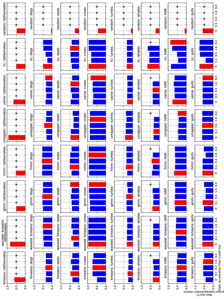
Figure S5: Hyperparameter optimization of static acceleration cutoff frequency (unsupervised models). Y-axis indicates the best F1 score on the test set of the fold used for hyperparameter optimization, chosen from all hyperparameter with the same cutoff frequency. A cross marker indicates that this dataset/model pair did not test hyperparameters for the cutoff. The hyperparameter chosen was not consistent within a dataset. Most models do not show large performance variation based on this hyperparameter.

References

- [1] Timo Adam, Christopher A. Griffiths, Vianey Leos-Barajas, Emily N. Meese, Christopher G. Lowe, Paul G. Blackwell, David Righton, and Roland Langrock, Joint modelling of multi-scale animal movement data using hierarchical hidden Markov models, Methods in Ecology and Evolution 10 (2019), no. 9, 1536–1550.
- [2] Enrique Amigó, Julio Gonzalo, Javier Artiles, and Felisa Verdejo, A comparison of extrinsic clustering evaluation metrics based on formal constraints, Information Retrieval 12 (2009), no. 4, 461–486.
- [3] Davide Anguita, Alessandro Ghio, Luca Oneto, Xavier Parra, and Jorge L Reyes-Ortiz, A Public Domain Dataset for Human Activity Recognition Using Smartphones, Computational Intelligence (2013), 6.
- [4] Melissa Bateson and Paul Martin, Measuring Behaviour: An Introductory Guide, Cambridge University Press, May 2021.
- [5] Sara Beery, Dan Morris, and Siyu Yang, Efficient pipeline for camera trap image review, Proceedings of the Workshop Data Mining and AI for Conservation (2019).
- [6] Oded Berger-Tal, Tal Polak, Aya Oron, Yael Lubin, Burt P. Kotler, and David Saltz, Integrating animal behavior and conservation biology: A conceptual framework, Behavioral Ecology 22 (2011), no. 2, 236–239.
- [7] Gordon J. Berman, William Bialek, and Joshua W. Shaevitz, Predictability and hierarchy in Drosophila behavior, Proceedings of the National Academy of Sciences of the United States of America 113 (2016), no. 42, 11943–11948.
- [8] Gordon J. Berman, Daniel M. Choi, William Bialek, and Joshua W. Shaevitz, Mapping the stereotyped behaviour of freely moving fruit flies, Journal of The Royal Society Interface 11 (2014), no. 99, 20140672.
- [9] Owen R. Bidder, Hamish A. Campbell, Agustina Gómez-Laich, Patricia Urgé, James Walker, Yuzhi Cai, Lianli Gao, Flavio Quintana, and Rory P. Wilson, Love Thy Neighbour: Automatic Animal Behavioural Classification of Acceleration Data Using the K-Nearest Neighbour Algorithm, PLOS ONE 9 (2014), no. 2, e88609.
- [10] James P Bohnslav, Nivanthika K Wimalasena, Kelsey J Clausing, Yu Y Dai, David A Yarmolinsky, Tomás Cruz, Adam D Kashlan, M Eugenia Chiappe, Lauren L Orefice, Clifford J Woolf, and Christopher D Harvey, DeepEthogram, a machine learning pipeline for supervised behavior classification from raw pixels, eLife 10 (2021), e63377.
- [11] Xavier Bouthillier, Pierre Delaunay, Mirko Bronzi, Assya Trofimov, Brennan Nichyporuk, Justin Szeto, Naz Sepah, Edward Raff, Kanika Madan, Vikram Voleti, Samira Ebrahimi Kahou, Vincent Michalski, Dmitriy Serdyuk, Tal Arbel, Chris Pal, Gaël Varoquaux, and Pascal Vincent, Accounting for Variance in Machine Learning Benchmarks, 23.
- [12] L. R. Brewster, J. J. Dale, T. L. Guttridge, S. H. Gruber, A. C. Hansell, M. Elliott, I. G. Cowx, N. M. Whitney, and A. C. Gleiss, Development and application of a machine learning algorithm for classification of elasmobranch behaviour from accelerometry data, Marine Biology 165 (2018), no. 4, 62.
- [13] Marianna Chimienti, Thomas Cornulier, Ellie Owen, Mark Bolton, Ian M. Davies, Justin M.J. Travis, and Beth E. Scott, The use of an unsupervised learning approach for characterizing latent behaviors in accelerometer data, Ecology and Evolution 6 (2016), no. 3, 727–741.
- [14] Thomas M. Clarke, Sasha K. Whitmarsh, Jenna L. Hounslow, Adrian C. Gleiss, Nicholas L. Payne, and Charlie Huveneers, Using tri-axial accelerometer loggers to identify spawning behaviours of large pelagic fish, Movement Ecology 9 (2021), no. 1, 26.
- [15] Sandeep Robert Datta, David J. Anderson, Kristin Branson, Pietro Perona, and Andrew Leifer, Computational neuroethology: A call to action, Neuron 104 (2019), no. 1, 11–24.
- [16] Nicholas B. Davies, John R. Krebs, and Stuart A. West, An Introduction to Behavioural Ecology, John Wiley & Sons, April 2012.
- [17] Stacy De Ruiter, Mark Johnson, Catriona Harris, Tiago Marques, René Swift, Yee Joo Oh, David Sweeney, and Lucía Martina Martín López, The animal tag tools project, 2020.
- [18] Mostafa Dehghani, Yi Tay, Alexey A Gritsenko, Zhe Zhao, Neil Houlsby, Fernando Diaz, Donald Metzler, and Oriol Vinyals, The benchmark lottery, arXiv preprint arXiv:2107.07002 (2021).
- [19] Stacy L. DeRuiter, Roland Langrock, Tomas Skirbutas, Jeremy A. Goldbogen, John Calambokidis, Ari S. Friedlaender, and Brandon L. Southall, A multivariate mixed hidden Markov model for blue whale behaviour and responses to sound exposure, The Annals of Applied Statistics 11 (2017), no. 1, 362 – 392.
- [20] Dominic L. DeSantis, Vicente Mata-Silva, Jerry D. Johnson, and Amy E. Wagler, Integrative Framework for Long-Term Activity Monitoring of Small and Secretive Animals: Validation With a Cryptic Pitviper, Frontiers in Ecology and Evolution 8 (2020).
- [21] Thomas G. Dietterich, Approximate statistical tests for comparing supervised classification learning algorithms, Neural Computation 10 (1998), 1895–1923.
- [22] Ewan Dunbar, Nicolas Hamilakis, and Emmanuel Dupoux, Self-supervised language learning from raw audio: Lessons from the zero resource speech challenge, IEEE Journal of Selected Topics in Signal Processing 16 (2022), no. 6, 1211–1226.
- [23] Anniek Eerdekens, Margot Deruyck, Jaron Fontaine, Luc Martens, Eli De Poorter, and Wout Joseph, Automatic equine activity detection by convolutional neural networks using accelerometer data, Computers and Electronics in Agriculture 168 (2020), 105139.
- [24] S.E. Roian Egnor and Kristin Branson, Computational Analysis of Behavior, Annual Review of Neuroscience 39 (2016), no. 1, 217–236.
- [25] Elena Eisenring, Marcel Eens, Jean-Nicolas Pradervand, Alain Jacot, Jan Baert, Eddy Ulenaers, Michiel Lathouwers, and Ruben Evens, Quantifying song behavior in a free-living, light-weight, mobile bird using accelerometers, Ecology and Evolution 12 (2022), no. 1, e8446.
- [26] Eyrun Eyjolfsdottir, Kristin Branson, Yisong Yue, and Pietro Perona, Learning recurrent representations for hierarchical behavior modeling, arXiv:1611.00094 [cs] (2016).
- [27] Clara Fannjiang, T. Aran Mooney, Seth Cones, David Mann, K. Alex Shorter, and Kakani Katija, Augmenting biologging with supervised machine learning to study in situ behavior of the medusa Chrysaora fuscescens, Journal of Experimental Biology 222 (2019), no. 16, jeb207654.
- [28] Gaelle Fehlmann, J.M. O’Riain, Phil Hopkins, Jack O’Sullivan, Mark Holton, Emily Shepard, and Andrew King, Identification of behaviours from accelerometer data in a wild social primate, Animal Biotelemetry 5 (2017).
- [29] Shai Fine, Yoram Singer, and Naftali Tishby, The hierarchical hidden markov model: Analysis and applications, Machine learning 32 (1998), no. 1, 41–62.
- [30] As Friedlaender, Rb Tyson, Ak Stimpert, Aj Read, and Dp Nowacek, Extreme diel variation in the feeding behavior of humpback whales along the western Antarctic Peninsula during autumn, Marine Ecology Progress Series 494 (2013), 281–289.
- [31] Konrad Gadzicki, Razieh Khamsehashari, and Christoph Zetzsche, Early vs late fusion in multimodal convolutional neural networks, 2020 IEEE 23rd International Conference on Information Fusion (FUSION), 2020, pp. 1–6.
- [32] Baptiste Garde, Rory P Wilson, Adam Fell, Nik Cole, Vikash Tatayah, Mark D Holton, Kayleigh AR Rose, Richard S Metcalfe, Hermina Robotka, Martin Wikelski, et al., Ecological inference using data from accelerometers needs careful protocols, Methods in Ecology and Evolution 13 (2022), no. 4, 813–825.
- [33] Peter Henderson, Jieru Hu, Joshua Romoff, Emma Brunskill, Dan Jurafsky, and Joelle Pineau, Towards the systematic reporting of the energy and carbon footprints of machine learning, Journal of Machine Learning Research 21 (2020), no. 248, 1–43.
- [34] J. D. Hunter, Matplotlib: A 2d graphics environment, Computing in Science & Engineering 9 (2007), no. 3, 90–95.
- [35] Nigel E. Hussey, Steven T. Kessel, Kim Aarestrup, Steven J. Cooke, Paul D. Cowley, Aaron T. Fisk, Robert G. Harcourt, Kim N. Holland, Sara J. Iverson, John F. Kocik, Joanna E. Mills Flemming, and Fred G. Whoriskey, Aquatic animal telemetry: A panoramic window into the underwater world, Science 348 (2015), no. 6240, 1255642.
- [36] Lorène Jeantet, Víctor Planas-Bielsa, Simon Benhamou, Sebastien Geiger, Jordan Martin, Flora Siegwalt, Pierre Lelong, Julie Gresser, Denis Etienne, Gaëlle Hiélard, Alexandre Arque, Sidney Regis, Nicolas Lecerf, Cédric Frouin, Abdelwahab Benhalilou, Céline Murgale, Thomas Maillet, Lucas Andreani, Guilhem Campistron, Hélène Delvaux, Christelle Guyon, Sandrine Richard, Fabien Lefebvre, Nathalie Aubert, Caroline Habold, Yvon le Maho, and Damien Chevallier, Behavioural inference from signal processing using animal-borne multi-sensor loggers: A novel solution to extend the knowledge of sea turtle ecology, Royal Society Open Science 7 (2020), no. 5, 200139.
- [37] Walter Jetz, Grigori Tertitski, Roland W. Kays, Uschi Mueller, Martin Wikelski, Susanne Åkesson, Yury Anisimov, Aleksey Antonov, Walter Arnold, Franz Bairlein, Oriol Baltà, Diane Baum, Mario Beck, O. A. Belonovich, Mikhail Belyaev, Matthias Berger, Peter Berthold, Steffen Bittner, Stephen Blake, Barbara Block, Daniel Bloche, Katrin Boehning-Gaese, Gil Bohrer, Julia Bojarinova, Gerhard Bommas, Oleg V. Bourski, A. V. Bragin, Alexander Bragin, Rachel M. Bristol, Vojtěch Brlík, Victor N. Bulyuk, Francesca Cagnacci, Ben Carlson, Taylor K. Chapple, Kalkidan F. Chefira, Yachang Cheng, Nikita Chernetsov, Grzegorz Cierlik, Simon S. Christiansen, Oriol Clarabuch, W. Cochran, Jamie M. Cornelius, Iain D. Couzin, Margret C. Crofoot, Sebastian Cruz, Alexander Davydov, Sarah C. Davidson, Stefan W. Dech, Dina K. N. Dechmann, E. A. Demidova, J. Dettmann, S Dittmar, Dmitry Ivanovich Dorofeev, Detlev Drenckhahn, V. M. Dubyanskiy, Nikolay Egorov, Sophie Ehnbom, Diego Ellis-Soto, Ralf Ewald, Christopher J. Feare, I. V. Fefelov, Péter Fehérvári, Wolfgang Fiedler, Andrea Flack, Magnus Froböse, Ivan A. Fufachev, Pavel Futoran, Vyachaslav Gabyshev, Anna Gagliardo, Stefan Garthe, Sergey B. Gashkov, Luke Gibson, Wolfgang Goymann, Gerd Gruppe, Christine T. Di Guglielmo, Ph. Hartl, Anders Hedenström, Arne Hegemann, George W. Heine, Mäggi Hieber Ruiz, Heribert Hofer, Felix Huber, Fabiola Iannarilli, Marc Illa, Arkadiy Isaev, Bent Karsten Jakobsen, Lukas Jenni, Susanne Jenni-Eiermann, Brett R. Jesmer, Frédéric Jiguet, T. Yu. Karimova, N. Jeremy Kasdin, Fedor Kazansky, R. A. Kirillin, Thomas Klinner, Andreas Knopp, Andrea Kölzsch, Alexander V. Kondratyev, Marco Krondorf, Pavel Ktitorov, Olga Kulikova, R. Suresh Kumar, Claudia Künzer, A. M. Larionov, Christine S. Larose, Felix Liechti, Nils Linek, Ashley Lohr, Anna A. Lushchekina, Kate Mansfield, Maria Matantseva, Mikhail Y. Markovets, Peter Marra, Juan F. Masello, Jörg Melzheimer, Myles H. M. Menz, Stephen Menzie, Swetlana G. Meshcheryagina, Dale G. Miquelle, Vladimir Morozov, Andrey Mukhin, Inge Müller, Thomas Mueller, Juan G. Navedo, Ran Nathan, Luke Nelson, Zoltán Németh, Scott Newman, Ryan Norris, Innokentiy M. Okhlopkov, Wioleta Oleś, Ruth Y. Oliver, T. M. O’mara, Péter Palatitz, Jesko Partecke, Ryan P Pavlick, A I Pedenko, Julie Pham, Daniel Piechowski, Allison K. Pierce, Theunis Piersma, Wolfgang Pitz, Dirk Plettemeier, Irina Pokrovskaya, Liya V. Pokrovskaya, Ivan G. Pokrovsky, Morrison T. Pot, Petr Procházka, Petra Quillfeldt, Eldar Rakhimberdiev, Marilyn Ramenofsky, Ajay Ranipeta, Jan Rapczyński, Magdalena Remisiewicz, V. B. Rozhnov, Froukje Rienks, V. B. Rozhnov, Christian Rutz, V. V. Sakhvon, Nir Sapir, Kamran Safi, Friedrich Schäuffelhut, David S. Schimel, Andreas Schmidt, Judy Shamoun-Baranes, A. I. Sharikov, Laura Baker Shearer, E. I. Shemyakin, Sherub Sherub, Ryan Shipley, Yanina V. Sica, T. B. Smith, Sergey Simonov, Katherine R. S. Snell, Aleksandr Sokolov, Vasiliy A. Sokolov, Olga Solomina, Mikhail Soloviev, Fernando Spina, Kamiel Spoelstra, Martin Storhas, T. V. Sviridova, George Swenson, Phil Taylor, Kasper Thorup, Arseny Tsvey, Marlee A. Tucker, Woody Turner, Henk P. van der Jeugd, Louis van Schalkwyk, Mariëlle L. van Toor, Pauli Viljoen, Marcel Erik Visser, Tamara Volkmer, Andrei Volkov, Sergey Volkov, Oleg Nikolaevich Volkov, Jan A. C. von Rönn, Bernd Vorneweg, Bettina Wachter, Jonas Waldenström, Martin Wegmann, Aloysius Wehr, Rolf P. Weinzierl, Johannes Weppler, David S Wilcove, Tim de Wild, Hannah J. Williams, John H. Wilshire, John Wingfield, Michael Wunder, Anna Yachmennikova, Scott W. Yanco, Elisabeth Yohannes, Amelie Zeller, Christian Ziegler, A. J. Ziecik, and Cheryl Zook, Biological earth observation with animal sensors., Trends in ecology & evolution 37 4 (2022), 293–298.
- [38] Xu Ji, Joao F. Henriques, and Andrea Vedaldi, Invariant information clustering for unsupervised image classification and segmentation, Proceedings of the IEEE/CVF International Conference on Computer Vision (ICCV), October 2019.
- [39] Mark P Johnson and Peter L Tyack, A digital acoustic recording tag for measuring the response of wild marine mammals to sound, IEEE journal of oceanic engineering 28 (2003), no. 1, 3–12.
- [40] Roland Kays, Margaret C. Crofoot, Walter Jetz, and Martin Wikelski, Terrestrial animal tracking as an eye on life and planet, Science 348 (2015), no. 6240, aaa2478.
- [41] Diederik P. Kingma and Jimmy Ba, Adam: A Method for Stochastic Optimization, 3rd International Conference on Learning Representations, ICLR 2015, San Diego, CA, USA, May 7-9, 2015, Conference Track Proceedings (Yoshua Bengio and Yann LeCun, eds.), 2015.
- [42] Joseph Korpela, Hirokazu Suzuki, Sakiko Matsumoto, Yuichi Mizutani, Masaki Samejima, Takuya Maekawa, Junichi Nakai, and Ken Yoda, Machine learning enables improved runtime and precision for bio-loggers on seabirds, Communications Biology 3 (2020), no. 1, 633.
- [43] Pekka Kumpulainen, Anna Valldeoriola Cardó, Sanni Somppi, Heini Törnqvist, Heli Väätäjä, Päivi Majaranta, Yulia Gizatdinova, Christoph Hoog Antink, Veikko Surakka, Miiamaaria V. Kujala, Outi Vainio, and Antti Vehkaoja, Dog behaviour classification with movement sensors placed on the harness and the collar, Applied Animal Behaviour Science 241 (2021), 105393.
- [44] Monique Ladds, Marcus Salton, David Hocking, Rebecca McIntosh, Adam Thompson, David Slip, and Rob Harcourt, Using accelerometers to develop time-energy budgets of wild fur seals from captive surrogates, PeerJ 6 (2018), e5814.
- [45] Monique Ladds, Adam Thompson, David Slip, David Hocking, and Rob Harcourt, Seeing it all: Evaluating supervised machine learning methods for the classification of diverse otariid behaviours, PLoS ONE 11 (2017), e0166898.
- [46] Yann LeCun, Yoshua Bengio, and Geoffrey Hinton, Deep learning, Nature 521 (2015), no. 7553, 436–444.
- [47] Vianey Leos-Barajas, Theoni Photopoulou, Roland Langrock, Toby A. Patterson, Yuuki Y. Watanabe, Megan Murgatroyd, and Yannis P. Papastamatiou, Analysis of animal accelerometer data using hidden Markov models, Methods in Ecology and Evolution 8 (2017), no. 2, 161–173.
- [48] Tsung-Yi Lin, Priya Goyal, Ross Girshick, Kaiming He, and Piotr Dollár, Focal loss for dense object detection, IEEE Transactions on Pattern Analysis and Machine Intelligence 42 (2020), no. 2, 318–327.
- [49] Scott Linderman, Benjamin Antin, David Zoltowski, and Joshua Glaser, SSM: Bayesian Learning and Inference for State Space Models, 10 2020.
- [50] Lucía Martina Martín López, Natacha Aguilar de Soto, Peter Teglberg Madsen, and Mark Johnson, Overall dynamic body acceleration measures activity differently on large versus small aquatic animals, Methods in Ecology and Evolution 13 (2020), 447 – 458.
- [51] Ilya Loshchilov and Frank Hutter, SGDR: Stochastic Gradient Descent with Warm Restarts, (2017).
- [52] Bogdan Ludusan, M Versteegh, Aren Jansen, Guillaume Gravier, Xuan-Nga Cao, Mark Johnson, and Emmanuel Dupoux, Bridging the gap between speech technology and natural language processing: An evaluation toolbox for term discovery systems, 10.
- [53] Kevin Luxem, Falko Fuhrmann, Johannes Kürsch, Stefan Remy, and Pavol Bauer, Identifying Behavioral Structure from Deep Variational Embeddings of Animal Motion, Preprint, Neuroscience, May 2020.
- [54] Christos Markos, James J. Q. Yu, and Richard Yi Da Xu, Capturing uncertainty in unsupervised gps trajectory segmentation using bayesian deep learning, Proceedings of the AAAI Conference on Artificial Intelligence 35 (2021), no. 1, 390–398.
- [55] Lucía Martina Martín López, Natacha Aguilar de Soto, Patrick Miller, and Mark Johnson, Tracking the kinematics of caudal-oscillatory swimming: a comparison of two on-animal sensing methods, Journal of Experimental Biology 219 (2016), no. 14, 2103–2109.
- [56] David W. McClune, Nikki J. Marks, Rory P. Wilson, Jonathan DR Houghton, Ian W. Montgomery, Natasha E. McGowan, Eamonn Gormley, and Michael Scantlebury, Tri-axial accelerometers quantify behaviour in the Eurasian badger (Meles meles): Towards an automated interpretation of field data, Animal Biotelemetry 2 (2014), no. 1, 5.
- [57] Leland McInnes, John Healy, and James Melville, UMAP: Uniform Manifold Approximation and Projection for Dimension Reduction, September 2020.
- [58] Ran Nathan, Orr Spiegel, Scott Fortmann-Roe, Roi Harel, Martin Wikelski, and Wayne M. Getz, Using tri-axial acceleration data to identify behavioral modes of free-ranging animals: General concepts and tools illustrated for griffon vultures, The Journal of Experimental Biology 215 (2012), no. 6, 986–996.
- [59] Francisco Javier Ordóñez and Daniel Roggen, Deep convolutional and lstm recurrent neural networks for multimodal wearable activity recognition, Sensors 16 (2016), no. 1.
- [60] Anthony Pagano, Metabolic Rate, Body Composition, Foraging Success, Behavior, and GPS Locations of Female Polar Bears (Ursus maritimus), Beaufort Sea, Spring, 2014-2016 and Resting Energetics of an Adult Female Polar Bear, 2018.
- [61] Anthony Pagano, Karyn Rode, Amy Cutting, S Jensen, Jasmine Ware, CT Robbins, GM Durner, Todd Atwood, Martyn Obbard, KR Middel, Gregory Thiemann, and Terrie Williams, Using tri-axial accelerometers to identify wild polar bear behaviors, Endangered Species Research 32 (2017).
- [62] Guansong Pang, Chunhua Shen, Longbing Cao, and Anton Van Den Hengel, Deep learning for anomaly detection: A review, ACM Comput. Surv. 54 (2021), no. 2.
- [63] Adam Paszke, Sam Gross, Francisco Massa, Adam Lerer, James Bradbury, Gregory Chanan, Trevor Killeen, Zeming Lin, Natalia Gimelshein, Luca Antiga, Alban Desmaison, Andreas Kopf, Edward Yang, Zachary DeVito, Martin Raison, Alykhan Tejani, Sasank Chilamkurthy, Benoit Steiner, Lu Fang, Junjie Bai, and Soumith Chintala, Pytorch: An imperative style, high-performance deep learning library, Advances in Neural Information Processing Systems (H. Wallach, H. Larochelle, A. Beygelzimer, F. d'Alché-Buc, E. Fox, and R. Garnett, eds.), vol. 32, Curran Associates, Inc., 2019.
- [64] Amandalynne Paullada, Inioluwa Deborah Raji, Emily M Bender, Emily Denton, and Alex Hanna, Data and its (dis) contents: A survey of dataset development and use in machine learning research, Patterns 2 (2021), no. 11, 100336.
- [65] F. Pedregosa, G. Varoquaux, A. Gramfort, V. Michel, B. Thirion, O. Grisel, M. Blondel, P. Prettenhofer, R. Weiss, V. Dubourg, J. Vanderplas, A. Passos, D. Cournapeau, M. Brucher, M. Perrot, and E. Duchesnay, Scikit-learn: Machine learning in Python, Journal of Machine Learning Research 12 (2011), 2825–2830.
- [66] Talmo D. Pereira, Joshua W. Shaevitz, and Mala Murthy, Quantifying behavior to understand the brain, Nature Neuroscience 23 (2020), no. 12, 1537–1549.
- [67] Inioluwa Deborah Raji, Emily M. Bender, Amandalynne Paullada, Emily Denton, and Alex Hanna, AI and the Everything in the Whole Wide World Benchmark, arXiv:2111.15366 [cs] (2021).
- [68] Yehezkel S. Resheff, Shay Rotics, Roi Harel, Orr Spiegel, and Ran Nathan, AcceleRater: A web application for supervised learning of behavioral modes from acceleration measurements, Movement Ecology 2 (2014), no. 1, 27.
- [69] Jorge-L Reyes-Ortiz, Luca Oneto, Albert Samà, Xavier Parra, and Davide Anguita, Transition-aware human activity recognition using smartphones, Neurocomputing 171 (2016), 754–767.
- [70] Olga Russakovsky, Jia Deng, Hao Su, Jonathan Krause, Sanjeev Satheesh, Sean Ma, Zhiheng Huang, Andrej Karpathy, Aditya Khosla, Michael Bernstein, Alexander C. Berg, and Li Fei-Fei, ImageNet Large Scale Visual Recognition Challenge, International Journal of Computer Vision 115 (2015), no. 3, 211–252.
- [71] Christian Rutz and Graeme C. Hays, New frontiers in biologging science, Biology Letters 5 (2009), no. 3, 289–292.
- [72] Christian Rutz and Jolyon Troscianko, Programmable, miniature video-loggers for deployment on wild birds and other wildlife, Methods in Ecology and Evolution 4 (2013), no. 2, 114–122.
- [73] Kentaro Q. Sakamoto, Katsufumi Sato, Mayumi Ishizuka, Yutaka Watanuki, Akinori Takahashi, Francis Daunt, and Sarah Wanless, Can Ethograms Be Automatically Generated Using Body Acceleration Data from Free-Ranging Birds?, PLOS ONE 4 (2009), no. 4, e5379.
- [74] Sarab S. Sethi, Nick S. Jones, Ben D. Fulcher, Lorenzo Picinali, Dena Jane Clink, Holger Klinck, C. David L. Orme, Peter H. Wrege, and Robert M. Ewers, Characterizing soundscapes across diverse ecosystems using a universal acoustic feature set, Proceedings of the National Academy of Sciences 117 (2020), no. 29, 17049–17055.
- [75] Judy Shamoun-Baranes, Roeland Bom, E. Emiel van Loon, Bruno J. Ens, Kees Oosterbeek, and Willem Bouten, From Sensor Data to Animal Behaviour: An Oystercatcher Example, PLoS ONE 7 (2012), no. 5, e37997.
- [76] Elc Shepard, Rp Wilson, F Quintana, A Gómez Laich, N Liebsch, Da Albareda, Lg Halsey, A Gleiss, Dt Morgan, Ae Myers, C Newman, and Dw McDonald, Identification of animal movement patterns using tri-axial accelerometry, Endangered Species Research 10 (2008), 47–60.
- [77] Laura Stidsholt, Mark Johnson, Kristian Beedholm, Lasse Jakobsen, Kathrin Kugler, Signe Brinkløv, Angeles Salles, Cynthia F Moss, and Peter Teglberg Madsen, A 2.6-g sound and movement tag for studying the acoustic scene and kinematics of echolocating bats, Methods in Ecology and Evolution 10 (2019), no. 1, 48–58.
- [78] Emily K. Studd, Manuelle Landry-Cuerrier, Allyson K. Menzies, Stan Boutin, Andrew G. McAdam, Jeffrey E. Lane, and Murray M. Humphries, Behavioral classification of low-frequency acceleration and temperature data from a free-ranging small mammal, Ecology and Evolution 9 (2019), no. 1, 619–630.
- [79] Maitreyi Sur, Tony Suffredini, Stephen M. Wessells, Peter H. Bloom, Michael Lanzone, Sheldon Blackshire, Srisarguru Sridhar, and Todd Katzner, Improved supervised classification of accelerometry data to distinguish behaviors of soaring birds, PLoS ONE 12 (2017), no. 4, e0174785.
- [80] Chris B. Thaxter, Ben Lascelles, Kate Sugar, Aonghais S.C.P. Cook, Staffan Roos, Mark Bolton, Rowena H.W. Langston, and Niall H.K. Burton, Seabird foraging ranges as a preliminary tool for identifying candidate marine protected areas, Biological Conservation 156 (2012), 53–61, Seabirds and Marine Protected Areas planning.
- [81] Andréa Thiebault, Chloé Huetz, Pierre Pistorius, Thierry Aubin, and Isabelle Charrier, Animal-borne acoustic data alone can provide high accuracy classification of activity budgets, Animal Biotelemetry 9 (2021), no. 1, 28.
- [82] Reid Tingley, Benjamin L. Phillips, Mike Letnic, Gregory P. Brown, Richard Shine, and Stuart J. E. Baird, Identifying optimal barriers to halt the invasion of cane toads rhinella marina in arid australia, Journal of Applied Ecology 50 (2013), no. 1, 129–137.
- [83] Devis Tuia, Benjamin Kellenberger, Sara Beery, Blair R. Costelloe, Silvia Zuffi, Benjamin Risse, Alexander Mathis, Mackenzie W. Mathis, Frank van Langevelde, Tilo Burghardt, Roland Kays, Holger Klinck, Martin Wikelski, Iain D. Couzin, Grant van Horn, Margaret C. Crofoot, Charles V. Stewart, and Tanya Berger-Wolf, Perspectives in machine learning for wildlife conservation, Nature Communications 13 (2022), no. 1, 792.
- [84] Ashish Vaswani, Noam Shazeer, Niki Parmar, Jakob Uszkoreit, Llion Jones, Aidan N. Gomez, Lukasz Kaiser, and Illia Polosukhin, Attention Is All You Need, arXiv:1706.03762 [cs] (2017).
- [85] Antti Vehkaoja, Sanni Somppi, Heini Törnqvist, Anna Valldeoriola Cardó, Pekka Kumpulainen, Heli Väätäjä, Päivi Majaranta, Veikko Surakka, Miiamaaria V. Kujala, and Outi Vainio, Description of movement sensor dataset for dog behavior classification, Data in Brief 40 (2022), 107822.
- [86] Jeffrey R. Walters, Scott R. Derrickson, D. Michael Fry, Susan M. Haig, John M. Marzluff, and Joseph M. Wunderle Jr., Status of the California Condor (Gymnogyps californianus) and Efforts to Achieve Its Recovery, The Auk 127 (2010), no. 4, 969 – 1001.
- [87] Guiming Wang, Machine learning for inferring animal behavior from location and movement data, Ecological Informatics 49 (2019), 69–76.
- [88] Rory Wilson, Emily Shepard, and Nikolai Liebsch, Prying into the intimate details of animal lives: Use of a daily diary on animals, Endangered Species Research 4 (2008), 123–137.
- [89] Alexander B. Wiltschko, Matthew J. Johnson, Giuliano Iurilli, Ralph E. Peterson, Jesse M. Katon, Stan L. Pashkovski, Victoria E. Abraira, Ryan P. Adams, and Sandeep Robert Datta, Mapping Sub-Second Structure in Mouse Behavior, Neuron 88 (2015), no. 6, 1121–1135.
- [90] Hui Yu, Jian Deng, Ran Nathan, Max Kröschel, Sasha Pekarsky, Guozheng Li, and Marcel Klaassen, An evaluation of machine learning classifiers for next-generation, continuous-ethogram smart trackers, Movement Ecology 9 (2021), no. 1, 15.