Diffusion-Based Speech Enhancement with
Joint Generative and Predictive Decoders

Abstract

Diffusion-based speech enhancement (SE) has been investigated recently, but its decoding is very time-consuming. One solution is to initialize the decoding process with the enhanced feature estimated by a predictive SE system. However, this two-stage method ignores the complementarity between predictive and diffusion SE. In this paper, we propose a unified system that integrates these two SE modules. The system encodes both generative and predictive information, and then applies both generative and predictive decoders, whose outputs are fused. Specifically, the two SE modules are fused in the first and final diffusion steps: the first step fusion initializes the diffusion process with the predictive SE for improving the convergence, and the final step fusion combines the two complementary SE outputs to improve the SE performance. Experiments on the Voice-Bank dataset show that the diffusion score estimation can benefit from the predictive information and speed up the decoding.

Index Terms: speech enhancement, diffusion model, generative model, predictive system

1 Introduction

Speech enhancement (SE) aims to recover clean speech from noisy signals. Since noise in real-world scenarios [1] significantly degrades the performance of speech applications, SE is an important front-end in speech processing applications [2, 3, 4]. Deep learning-based supervised SE systems [5, 6] have more robust performance compared to traditional SE systems [7, 8]. Therefore, the deep-learning-based methods to improve SE systems have recently been intensively investigated [9, 10].

Deep-learning-based SE systems can be classified into two types: predictive (also called discriminative) [11, 12, 13, 14] and generative [15, 16, 17, 18]. They adopt different paradigms. Predictive SE systems learn the single best deterministic mapping between noisy speech and its corresponding clean speech [18]. On the other hand, the target distribution is implicitly or explicitly learned in generative SE systems [18]. Generative SE models include variational auto-encoders [19], generative adversarial networks [15] and diffusion models [16, 17, 18]. Among them, diffusion models have recently attracted a significant attention due to their success in other fields [20, 21].

Diffusion models are inspired by non-equilibrium thermodynamics. The data are gradually turned into noise, and the neural network learns to invert the progressive noise-adding process. The two main frameworks are the conditional diffusion model [16] and the score-based diffusion model [17]. The conditional diffusion model uses noisy spectrograms as the conditioner. However, its objective function assumes that the global distribution of the additive noise follows a standard white Gaussian distribution, which is inconsistent with real noise statistics. The score-based diffusion model is based on stochastic differential equations (SDEs), which makes the training fully generative without any prior noise distribution assumptions.

The reverse diffusion process (decoding) of the diffusion models is very time-consuming. Although several studies [18, 22] have combined a predictive model with the generative model to reduce the number of reverse diffusion steps significantly, the predictive information is only used as the initialization information for the generative model. It has been shown that the generative and predictive models have different distortions [18]. Furthermore, UNIVERSE [23] shows that adding predictive information to the decoder of the diffusion model can help diffusion score estimation. However, the previous systems [18, 22] combining the generative and predictive combination models ignore the complementarity between them.

In this paper, we propose a unified SE system that integrates the generative and predictive SE modules. The model shares one encoder and contains predictive and generative decoders. The generative module is a score-based diffusion model adopted in the predictor-corrector (PC) samplers [24]. In this way, the model simultaneously outputs a score and enhanced predictive features. The enhanced generative-based and predictive-based features are fused in the first and final diffusion step. The first step fusion utilizes the predicted enhanced feature to initialize the subsequent diffusion processes. In order to maintain small changes in the feature distribution, the two features are fused instead of using the predicted spectra directly, although the enhanced predictive feature has higher performance in the first step than the enhanced generative feature. Since the two systems introduce different signal distortions, feature fusion is also adopted in the final step to leverage the complementarity between the generative and predictive SE modules.

2 Score-based Diffusion Model

2.1 Stochastic process

The linear stochastic differential equation (SDE) relies on a stochastic diffusion process $\left\{x_{t}\right\}_{t=0}^{T}$ [24]:

$$\mathrm{d}x_{t}=\underset{:=\mathrm{f}(x_{t},y)}{\underbrace{\gamma(y-x_{t})\mathrm{d}t}}+\underset{:=g(t)}{\underbrace{\left[\sigma_{min}(\frac{\sigma_{max}}{\sigma_{min}})^{t}\sqrt{2\mathrm{log}(\frac{\sigma_{max}}{\sigma_{min}})}\right]}}\mathrm{d}\mathrm{w}$$ (1)

where $x_{t}$ is the current state of the process indexed by a continuous time variable $t\in\left[0,T\right]$ [24]. $x_{0}$ is the clean speech, which represents the initial condition, $y$ is the noisy speech, and $\mathrm{w}$ denotes a standard Wiener process. The vector-valued function $\mathrm{f}(x_{t},y)$ is referred to as the drift coefficient, $g(t)$ is the diffusion coefficient of $x_{t}$, and $\gamma$ is the stiffness. $\sigma_{min}$ and $\sigma_{max}$ control the amount of Gaussian white noise at each diffusion timestep. The SDE in (1) has an associated reverse SDE [24, 25],

$$\mathrm{d}x_{t}=\left[-\mathrm{f}(x_{t},y)+g(t)^{2}\bigtriangledown_{x_{t}}\mathrm{log}p_{t}(x_{t})\right]\mathrm{d}t+g(t)\mathrm{d}\bar{\mathrm{w}}$$ (2)

where the score $\bigtriangledown_{x_{t}}\mathrm{log}p_{t}(x_{t})$ is estimated by a score model. The score model can be denoted as $s_{\theta}(x_{t},y,t)$, which is parameterized by a set of DNN parameters $\theta$. It receives the current state of the process $x_{t}$, the noisy speech $y$, and the current timestep $t$ as inputs. Finally, by substituting the score model into the reverse SDE in (2) [26], we obtain

$$\mathrm{d}x_{t}=\left[-\mathrm{f}(x_{t},y)+g(t)^{2}s_{\theta}(x_{t},y,t)\right]\mathrm{d}t+g(t)\mathrm{d}\bar{\mathrm{w}}]$$ (3)

which can be solved with various solver procedures.

2.2 Training objective

The mean and variance of the process state $x_{t}$ can be derived when its initial conditions are known [27]. Since the feature used in this paper is a complex spectrogram, at an arbitrary timestep $t$, $x_{t}$ can be directly sampled by $x_{0}$ and $y$ with the perturbation kernel:

$$p_{0t}(x_{t}|x_{0},y)=\mathcal{CN}_{\mathbb{c}}(x_{t};\mu(x_{0},y,t),\sigma(t)^{2}\mathrm{I})$$ (4)

where $\mathcal{CN}_{\mathbb{c}}$ denotes the circularly symmetric complex normal distribution. $\mathrm{I}$ is the identiry matrix. The mean and variance can be estimated as follows [27]:

$$\mu\left(x_{0},y,t\right)=e^{-\gamma t}x_{0}+(1-e^{-\gamma t})y$$ (5)

$$\sigma(t)^{2}=\frac{\sigma^{2}_{min}((\sigma_{max}/\sigma_{min})^{2t}-e^{-2\gamma t})\mathrm{log}(\sigma_{max}/\sigma_{min})}{\gamma+\mathrm{log}(\sigma_{max}/\sigma_{min})}$$ (6)

The denoising score matching is described as follows [17]:

$$\bigtriangledown_{x_{t}} \mathrm{log}p_{0t}(x_{t}|x_{0},y)=\bigtriangledown_{x_{t}}\mathrm{log}\left[\left|2\pi\sigma\mathrm{I}\right|^{-\frac{1}{2}}e^{-\frac{||x_{t}-\mu||^{2}_{2}}{2\sigma^{2}}}\right]$$ (7)

$$=\bigtriangledown_{x_{t}}\mathrm{log}\left|2\pi\sigma(t)\mathrm{I}\right|^{-\frac{1}{2}}-\bigtriangledown_{x_{t}}\frac{||x_{t}-\mu(x_{0},y,t)||^{2}_{2}}{2\sigma(t)^{2}}$$

$$=-\frac{x_{t}-\mu(x_{0},y,t)}{\sigma(t)^{2}}$$

At each training step, the following four steps are executed [17]:

1. Sample a random $t\sim\mathcal{U}\left[t_{\varepsilon},T\right]$;

2. Sample $(x_{0},y)$ from the dataset;

3. Sample $\mathrm{z}\sim\mathcal{CN}(\mathrm{z};0,\mathrm{I})$;

4. Sample $x_{t}$ from (4) by computing:

   $$x_{t}=\mu(x_{0},y,t)+\sigma(t)\mathrm{z}$$ (8)

The training loss is computed between the model output and the score of the perturbation kernel. By substituting (8) into (7), the overall training objective is described as follows [17]:

$$\underset{\theta}{\mathrm{arg}~{}\mathrm{min}\,}\mathbb{E}_{t,(x_{0},y),\mathrm{z},x_{t}|(x_{0},y)}\left[||\mathrm{s}_{\theta}(x_{t},y,t)+\frac{\mathrm{z}}{\sigma(t)}||^{2}_{2}\right]$$ (9)

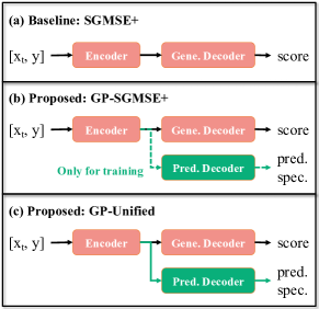
Figure 1: The score model (used in PC samplers) structure:
(a) the baseline SGMSE+; (b) the proposed Generative and Predictive based SGMSE+ (GP-SGMSE+); (c) the proposed Unified Generative and Predictive model (GP-Unified). Note that the skip connection exists between the encoder and decoders (generative and predictive).

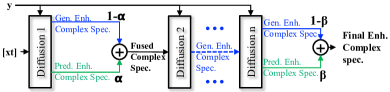
Figure 2: A flowchart of the proposed method. Generative and predictive SE systems are fused in the first and final diffusion steps.

2.3 Inference

For inference, a trained score model $\mathrm{s}_{\theta}$ approximates the true score for all $t\in\left[0,T\right]$. The noisy speech $y$ is conditioned to estimate clean speech $x_{0}$ by solving the plug-in reverse SDE in (3). The initial condition of the reverse process at $t=T$ can be determined as follows [17]:

$$x_{T}\sim\mathcal{N}_{\mathbb{C}}(x_{T};y,\sigma(T)^{2}\mathrm{I})$$ (10)

The denoising process through the reverse process starts at $t=T$ and ends at $t=0$ iteratively. PC samplers combine single-step methods with numerical optimization approaches for the reverse SDE [24]. PC samplers consist of a predictor and a corrector. The predictor solves the reverse process by iterating through the reverse SDE [24]. The corrector refines the current state after each iteration step of the predictor [24].

3 Proposed Method

Score-based diffusion models have already achieved performance comparable to that of the predictive model. However, the predictive model calls the neural network only once, while the diffusion model needs to call the neural network several times, which significantly increases the decoding time. Some multi-stage models incorporate enhanced predictive features into the diffusion model to significantly reduce the number of diffusion steps. However, these systems ignore the complementarity in the feature level between the predictive and generative models, since the generative models distort signals much differently from how the predictive models do [18]. Besides, introducing predictive information into generative models can help improve the performance of the diffusion process [23]. Therefore, we implement these two different SE systems in the unified system by fusing them. The flowchart of the proposed method is shown in Fig. 2.

3.1 GP-SGMSE+

The structure of the generative- and predictive-based model (GP-SGMSE+) to estimate a score $\bigtriangledown_{x_{t}}\mathrm{log}p_{t}(x_{t})$ is shown in Fig. 1(b). The model contains a shared encoder and two decoders. In this model, the predictive decoder is only used during training to introduce predictive enhancement information into the model. When decoding, no additional parameters are introduced to the baseline model shown in Fig. 1(a). The mean square error is used for computing the predictive loss:

$$L_{pred}=||x_{pred}-x_{0}||^{2}$$ (11)

where $x_{pred}$ is the output of the predictive decoder. The final loss combines both the predictive and generative loss in (9) and (11). Because the two tasks are equally important, the weights of the losses of the two parts are 0.5 during training. The weights of the losses will not affect the two separate decoders, but will affect the shared encoder information, which will be explored in the future. During decoding, only the generative decoder is used. The inference process is the same as in Section 2.3.

3.2 GP-Unified

The structure of the unified generative and predictive model (GP-Unified) is shown in Fig. 1(c). Unlike in ``GP-SGMSE+'', the predictive decoder is also used in the decoding. During the decoding, the enhanced generative and predictive features are fused in the first and final diffusion steps. The first step fusion is to use the predictive enhanced spectrogram to initialize the follow-up processes of diffusion:

$$\widehat{x_{1}}=\alpha*x_{1}+(1-\alpha)*x_{1}^{pre}$$ (12)

where $\widehat{x_{1}}$ is the first diffusion-enhanced complex spectrogram, which will be used for subsequent diffusion steps, and $x_{1}^{pre}$ is the predictive enhanced complex spectrogram in the first diffusion step. The reason for not using the predicted complex spectrogram directly is to maintain the feature distribution of the diffusion complex spectrograms. The two enhanced complex spectrograms are fused in the final step to exploit the complementary information:

$$\widehat{x_{n}}=\beta*x_{n}+(1-\beta)*x_{n}^{pre}$$ (13)

where $\widehat{x_{n}}$ is the final enhanced feature, and $x_{n}^{pre}$ is the predictive enhanced feature in the final diffusion step. The first and final fusion are only used for decoding. The final loss combines both predictive and generative loss in (9) and (11).

4 Experimental Evaluations

The Noise Conditional Score Network (NCSN++) architecture was used for the score model in both the baseline model (SGMSE+) and the proposed models (GP-SGMSE+, GP-Unified). The generative and predictive decoders had the same structure. The real and imaginary parts of the complex spectrograms were used as inputs. The residual blocks in upsampling and downsampling layers were based on the BigGAN architecture. Each upsampling layer consisted of three residual blocks, and each downsampling layer consisted of two blocks with the last block performing the upsampling or downsampling. Global attention was added at a resolution of $16\times 16$ and in the bottleneck layer. All models were trained for 100 epochs.

The experiments were based on the public Voicebank-DEMAND [28]. The dataset can be accessed from this URL. All speech data were sampled at 16 kHz.

To evaluate the proposed method, perceptual evaluation of speech quality (PESQ) [29], extended short-time objective intelligibility (ESTOI) [30], scale-invariant signal-to-distortion ratio (SI-SDR) [31], scale-invariant signal-to-interference ratio (SI-SIR) [31], and scale-invariant signal-to-artifact ratio (SI-SAR) [31] are used as the evaluation metric.

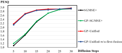
Figure 3: PESQ performance with different diffusion steps

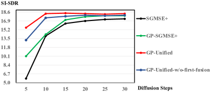
Figure 4: SI-SDR performance with different diffusion steps

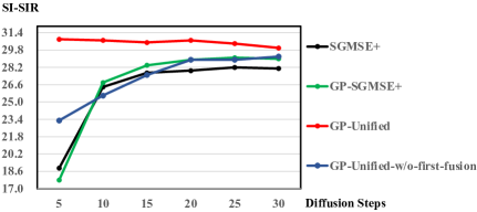
Figure 5: SI-SIR performance with different diffusion steps

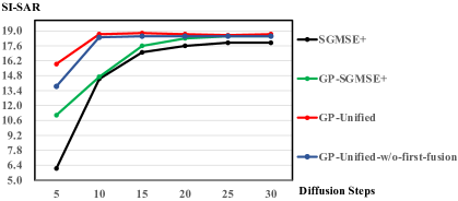
Figure 6: SI-SAR performance with different diffusion steps

We set the hyperparameter $\alpha$ for the first step fusion from 0.1 to 0.9, and finally found that 0.2 was the best. The hyperparameter $\beta$ for the final step fusion was 0.1. Because the two tasks are equally important, the weights of the training losses of the two parts are 0.5. We also tried fusing complex spectrograms at each step, but did not obtain improved performance.

4.1 Effect of incorporating predictive loss function

As shown by comparison of ``SGMSE+'' and ``GP-SGMSE+'' in Figure 6 to Figure 6, introducing a predictive loss function into the diffusion model can effectively reduce speech distortion, reduce noise, and reduce artificial noise. However, the predictive information has a minor effect on the PESQ, as shown in Figure 6.

Table 1: PESQ performance of the predictive output of ``GP-Unified'' in different diffusion steps.

Diffusion steps	5	10	15	20	25	30
PESQ	2.16	2.67	2.85	2.91	2.93	2.95

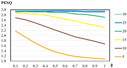
Figure 7: PESQ performance of ``GP-Unified'' under different diffusion steps with different $\beta$.

4.2 Effect of the first fusion

``GP-Unified-w/o-first-fusion'' adopts only the final fusion without the first diffusion-iteration fusion. As shown by the comparison of ``GP-Unified'' and ``GP-Unified-w/o-first-fusion'' in Fig. 6 and 6, the first step fusion mainly affects the diffusion speed. Besides, Fig. 6 shows that the ``GP-Unified'' outperforms ``GP-Unified-w/o-first-fusion'' even though the model already has large diffusion steps. This implies that the first step fusion not only plays the role of initialization but also compensates for some speech distortion caused by diffusion.

4.3 Effect of the final fusion

``GP-SGMSE+'' and ``GP-Unified-w/o-first-fusion'' were trained by the same manner; the difference lies in whether they are fused in the final diffusion step. The final fusion step gives a significant PESQ improvement, especially when the number of diffusion steps is small, as shown in Fig. 6. Furthermore, the final step fusion can significantly reduce speech distortion (Fig. 6) and artificial noise (Fig. 6) when the number of steps is small. However, the effect is not obvious for noise suppression (Fig. 6). Table 1 shows the performance of the predictive output at different diffusion steps. The performance improves as the iteration steps increases. The proposed system can combine the characteristics of predictive and generative SE and fully use the predictive complex spectrograms even when the number of diffusion steps is small. When the diffusion steps increase, the complementarity between the generative and predicted complex spectrograms is manifested. Through the fusion, PESQ and SI-SDR can be further improved, as shown in Fig. 6 and 6.

4.4 Effect of fusion hyperparameter $\beta$

Figure 7 shows the PESQ performance of ``GP-Unified'' under several diffusion steps with different values of $\beta$. $\beta$ has a more significant impact on smaller diffusion steps, and the advantages of the fusion are mainly reflected for smaller diffusion steps, especially in steps 5, 10, and 15. In step 5, the main performance improvement comes from predictive information. In steps 10, 15, and 20, it mainly comes from the feature fusion: the performance of ``GP-Unified'' was improved compared to the generative (``GP-SGMSE+'') and the predictive model (results shown in the Table 2). Their difference lies in the feature fusion.

Table 2: Performance of different speech enhancement systems in VB dataset: ``Type'' denotes the type of the system, ``P'' represents the predictive model, ``G'' represents the generative model.

System	Type	PESQ	ESTOI	SI-SDR
Mixture	-	1.97	0.79	8.4
Conv-Tasnet [13]	P	2.84	0.85	19.1
MetricGAN+ [12]	P	3.13	0.83	8.5
GaGNet [14]	P	2.94	0.86	19.9
SEGAN [15]	G	2.16	-	-
CDiffuSE [16]	G	2.46	0.79	12.6
SGMSE+ [17]	G	2.93	0.87	17.3
StoRM [18]	G	2.93	0.88	18.8
UNIVERSE	G	2.91	0.84	10.1
GP-SGMSE+	G	2.95	0.87	17.9
GP-Unified	G	2.97	0.87	18.3

Table 3: Total parameters of different diffusion models.

System	SGMSE+	StoRM	GP-Unified
Parameters	65.6M	125M	106M

The system performs better when $\beta$ is smaller, which means that the generative information is incorporated into the predictive complex spectrogram.

4.5 Comparasion with other methods

Comparison with other methods, including ``StoRM'' and ``UNIVERSE'', are listed in Table 2. Compared with the proposed method, ``UNIVERSE'' significantly degraded SI-SDR. This suggests that incorporating predictive information by the form of ``UNIVERSE'' is not beneficial to improving segment-level performance. Compared with ``StoRM'', the proposed method had better PESQ performance. This suggests that the proposed method can achieve better frequency-domain enhancement performance, since PESQ depends on the frequency-domain performance. Moreover, the number of parameters of our proposed method is much smaller than ``StoRM'', as shown in Table LABEL:paramteres.

5 Conclusions and Future Works

In this paper, we have proposed a unified generative and predictive speech enhancement model (GP-Unified). The model encodes both generative and predictive information and applies the generative and predictive decoders separately, whose results are fused. The predictive information helps the model to reduce speech distortion, noise, and artifacts. The two systems are fused in the first and final steps. The information fusion can speed up the diffusion process by reducing the number of diffusion steps by about 50%. Besides, information fusion can lead to better performance with the complementary between the predictive and generative SE.

References

- [1] J. Li, L. Deng, Y. Gong, and R. Haeb-Umbach, ``An Overview of Noise-Robust Automatic Speech Recognition,'' IEEE/ACM TASLP, vol. 22, no. 4, pp. 745–777, 2014.
- [2] A. Maas, Q. V. Le, T. M. O’Neil, O. Vinyals, P. Nguyen, and A. Y. Ng, ``Recurrent Neural Networks for Noise Reduction in Robust ASR,'' in Proc. INTERSPEECH, 2012.
- [3] A. Narayanan and D. Wang, ``Ideal ratio mask estimation using deep neural networks for robust speech recognition,'' in Proc. ICASSP, 2013, pp. 7092–7096.
- [4] M. Mimura, S. Sakai, and T. Kawahara, ``Exploring deep neural networks and deep autoencoders in reverberant speech recognition,'' in Proc. HSCMA, 2014, pp. 197–201.
- [5] Z.-Q. Wang, P. Wang, and D. Wang, ``Complex Spectral Mapping for Single- and Multi-Channel Speech Enhancement and Robust ASR,'' IEEE/ACM TASLP, vol. 28, pp. 1778–1787, 2020.
- [6] Y. Xu, J. Du, L.-R. Dai, and C.-H. Lee, ``A Regression Approach to Speech Enhancement Based on Deep Neural Networks,'' IEEE/ACM TASLP, vol. 23, no. 1, pp. 7–19, 2015.
- [7] S. Kamath and P. Loizou, ``A multi-band spectral subtraction method for enhancing speech corrupted by colored noise,'' in Proc. ICASSP, vol. 4, 2002, pp. IV–4164–IV–4164.
- [8] Y. Ephraim and H. Van Trees, ``A signal subspace approach for speech enhancement,'' IEEE Transactions on Speech and Audio Processing, vol. 3, no. 4, pp. 251–266, 1995.
- [9] D. Yin, C. Luo, Z. Xiong, and W. Zeng, ``PHASEN: A Phase-and-Harmonics-Aware Speech Enhancement Network,'' Proc. AAAI, vol. 34, no. 05, pp. 9458–9465, 2020.
- [10] M. Kolbæk, Z.-H. Tan, S. H. Jensen, and J. Jensen, ``On Loss Functions for Supervised Monaural Time-Domain Speech Enhancement,'' IEEE/ACM TASLP, vol. 28, pp. 825–838, 2020.
- [11] H. Shi, L. Wang, M. Ge, S. Li, and J. Dang, ``Spectrograms Fusion with Minimum Difference Masks Estimation for Monaural Speech Dereverberation,'' in Proc. ICASSP, 2020, pp. 7544–7548.
- [12] S.-W. Fu, C. Yu, T.-A. Hsieh, P. Plantinga, M. Ravanelli, X. Lu, and Y. Tsao, ``Metricgan+: An improved version of metricgan for speech enhancement,'' 2021. [Online]. Available: https://arxiv.org/abs/2104.03538
- [13] Y. Luo and N. Mesgarani, ``Conv-tasnet: Surpassing ideal time–frequency magnitude masking for speech separation,'' IEEE/ACM TASLP, vol. 27, no. 8, pp. 1256–1266, 2019.
- [14] A. Li, C. Zheng, L. Zhang, and X. Li, ``Glance and gaze: A collaborative learning framework for single-channel speech enhancement,'' Applied Acoustics, vol. 187, p. 108499, 2022.
- [15] S. Pascual, A. Bonafonte, and J. Serrà, ``SEGAN: Speech Enhancement Generative Adversarial Network,'' in Proc. Interspeech, 2017, pp. 3642–3646.
- [16] Y.-J. Lu, Z.-Q. Wang, S. Watanabe, A. Richard, C. Yu, and Y. Tsao, ``Conditional Diffusion Probabilistic Model for Speech Enhancement,'' in Proc. ICASSP, 2022, pp. 7402–7406.
- [17] J. Richter, S. Welker, J.-M. Lemercier, B. Lay, and T. Gerkmann, ``Speech Enhancement and Dereverberation with Diffusion-based Generative Models.'' arXiv, 2022.
- [18] J.-M. Lemercier, J. Richter, S. Welker, and T. Gerkmann, ``StoRM: A Diffusion-based Stochastic Regeneration Model for Speech Enhancement and Dereverberation.'' arXiv, 2022.
- [19] S. Leglaive, L. Girin, and R. Horaud, ``A variance modeling framework based on variational autoencoders for speech enhancement,'' in Proc. MLSP, 2018, pp. 1–6.
- [20] Y. Song and S. Ermon, ``Generative modeling by estimating gradients of the data distribution,'' in Proc. NIPS, H. Wallach, H. Larochelle, A. Beygelzimer, F. d'Alché-Buc, E. Fox, and R. Garnett, Eds., vol. 32. Curran Associates, Inc., 2019.
- [21] D. Kingma, T. Salimans, B. Poole, and J. Ho, ``Variational diffusion models,'' in Proc. NIPS, M. Ranzato, A. Beygelzimer, Y. Dauphin, P. Liang, and J. W. Vaughan, Eds., vol. 34. Curran Associates, Inc., 2021, pp. 21 696–21 707.
- [22] R. Sawata, N. Murata, Y. Takida, T. Uesaka, T. Shibuya, S. Takahashi, and Y. Mitsufuji, ``A versatile diffusion-based generative refiner for speech enhancement.'' arXiv, 2022.
- [23] J. Serrà, S. Pascual, J. Pons, R. O. Araz, and D. Scaini, ``Universal Speech Enhancement with Score-based Diffusion.'' arXiv, 2022.
- [24] Y. Song, J. Sohl-Dickstein, D. P. Kingma, A. Kumar, S. Ermon, and B. Poole, ``Score-based generative modeling through stochastic differential equations,'' in Proc. ICLR, 2021.
- [25] B. D. Anderson, ``Reverse-time diffusion equation models,'' Stochastic Processes and their Applications, vol. 12, no. 3, pp. 313–326, 1982.
- [26] C.-W. Huang, J. H. Lim, and A. C. Courville, ``A variational perspective on diffusion-based generative models and score matching,'' in Proc. NIPS, vol. 34, 2021, pp. 22 863–22 876.
- [27] B. Øksendal, Stochastic Differential Equations. Springer Berlin Heidelberg, 2003, pp. 65–84.
- [28] C. Valentini-Botinhao, X. Wang, S. Takaki, and J. Yamagishi, ``Investigating rnn-based speech enhancement methods for noise-robust text-to-speech.'' in Proc. SSW, 2016, pp. 146–152.
- [29] A. W. Rix, J. G. Beerends, M. P. Hollier, and A. P. Hekstra, ``Perceptual evaluation of speech quality (PESQ)-a new method for speech quality assessment of telephone networks and codecs,'' in Proc. ICASSP, vol. 2, 2001, pp. 749–752 vol.2.
- [30] J. Jensen and C. H. Taal, ``An algorithm for predicting the intelligibility of speech masked by modulated noise maskers,'' IEEE/ACM TASLP, vol. 24, no. 11, pp. 2009–2022, 2016.
- [31] J. L. Roux, S. Wisdom, H. Erdogan, and J. R. Hershey, ``Sdr – half-baked or well done?'' in Proc. ICASSP, 2019, pp. 626–630.