BlindHarmony: “Blind” Harmonization for MR Images via Flow model

Abstract

In MRI, images of the same contrast (e.g., T₁) from the same subject can exhibit noticeable differences when acquired using different hardware, sequences, or scan parameters. These differences in images create a domain gap that needs to be bridged by a step called image harmonization, to process the images successfully using conventional or deep learning-based image analysis (e.g., segmentation). Several methods, including deep learning-based approaches, have been proposed to achieve image harmonization. However, they often require datasets from multiple domains for deep learning training and may still be unsuccessful when applied to images from unseen domains. To address this limitation, we propose a novel concept called ‘Blind Harmonization’, which utilizes only target domain data for training but still has the capability to harmonize images from unseen domains. For the implementation of blind harmonization, we developed BlindHarmony using an unconditional flow model trained on target domain data. The harmonized image is optimized to have a correlation with the input source domain image while ensuring that the latent vector of the flow model is close to the center of the Gaussian distribution. BlindHarmony was evaluated on both simulated and real datasets and compared to conventional methods. BlindHarmony demonstrated noticeable performance on both datasets, highlighting its potential for future use in clinical settings. The source code is available at: https://github.com/SNU-LIST/BlindHarmony

1 Introduction

Magnetic resonance imaging (MRI) is a widely-used medical imaging modality. With the advent of deep learning-based computer vision techniques, there have been numerous applications of deep learning in MRI, such as disease classification [5, 36, 23], tumor segmentation [3, 46], and solving inverse problems [18, 44]. Despite the notable performance of deep learning in MRI, its widespread use has been hindered by the inherent domain gap present in MRI data [6, 8]. Variations occur in MRI images across different vendors, scanners, sites, and scan parameters even when the images are acquired from the same subject. This domain gap presents a generalization problem when applying the data to a neural network that has been trained on a different dataset.

To overcome the challenges of generalization in deep learning applied to MRI data, several harmonization methods have been developed to match the source domain image to the characteristics of the target domain. These approaches include non-deep learning-based methods [37, 31, 38, 29, 34, 15] and deep learning-based methods [9, 30, 26, 10, 13, 17], which have demonstrated performance improvements. However, there are limitations that need to be addressed. Firstly, many of these methods require multiple datasets from different domains. For instance, DeepHarmony [9] which is a supervised end-to-end framework requires “traveling subjects” who undergo multiple MRI scans with different scanners to obtain images from both the source and target domains. Utilizing CycleGAN-based style transfer can mitigate the need for traveling subjects [30, 26], but it still necessitates large datasets with multiple domains. Secondly, the harmonization network trained for mapping between specific source and target domains is challenging to be applied in unseen domains, limiting the generalizability of methods. Efforts have been made to employ disentanglement approaches or domain adaptation to achieve harmonization in unseen domains, but it requires a multi-contrast or multi-site paired dataset [10, 48]. To overcome these challenges, we propose the concept of “Blind Harmonization”, where the harmonization network can be constructed only with the target domain data during training and applicable to diverse source domains that are unseen during training.

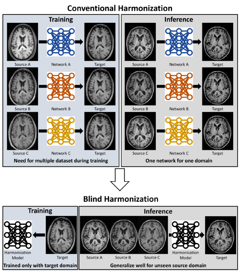
Figure 1: Blind harmonization presents an advantage over conventional harmonization models. While traditional models often necessitate multiple datasets during training or show reduced performance on unseen domains, blind harmonization can be trained solely with target domain data and generalized to previously unseen source domains.

In recent years, a class of invertible generative models called normalizing flow [11, 21, 12] has been introduced and has shown exceptional performance in a wide range of computer vision tasks [27, 2, 33]. Normalizing flow has the unique ability not only to generate novel images that resemble samples from the distribution of a given dataset but also to map the probabilistic distribution of image datasets. This feature makes normalizing flows particularly well-suited for image generation and manipulation tasks, as they can effectively capture the underlying distribution of image data and generate new images that are consistent with that distribution. Furthermore, the invertibility of these models provides fine-grained control over the generated images, making them useful for tasks such as image manipulation and style transfer. [1, 41]

In this paper, as a solution for blind harmonization, we introduce BlindHarmony which is a flow-based blind MR image harmonization framework that uses only the target domain dataset during training. Our method aims to find the harmonized image that preserves the anatomical structure and contrast of the input source domain image while maintaining a high likelihood in the flow model (i.e., enabling harmonization for the target domain), leveraging the invertibility of flow models. Our contributions are as follows:

1. We present the concept of blind harmonization, which does not require the source domain data during training and can perform harmonization for the images of untrained domains.

2. As an implementation of blind harmonization, we propose BlindHarmony. In BlindHarmony, the flow model is trained solely with the target domain data, and the harmonized image is optimized by leveraging the invertibility of the flow model.

3. We evaluate our method on both simulated data and real-world data.

2 Related works

2.1 MRI harmonization

There are numerous demands for harmonizing MR images from different sites, vendors, or scanners. Several studies have proposed methods for harmonizing MR images from the source domain to the target domain. Conventionally, these approaches have relied on image-level post-processing techniques, such as histogram matching [38, 32, 31] and statistical normalization [15, 34, 37], which aim to adjust the intensity values of the images to make them more similar. However, conventional methods had difficulty in capturing the subtle differences between images from different domains. For example, histogram-based models assume global histogram correspondence between images, so they ignore local contrast information. With recent advances in deep learning, there has been growing interest in developing deep learning-based methods for harmonization. One popular deep learning-based method is DeepHarmony [9], which utilizes an end-to-end supervised framework to learn the mapping between the source and target domains. Although DeepHarmony has demonstrated promising results, it requires a large dataset of traveling subjects for training, which is difficult to acquire. To address this limitation, CycleGAN-based style transfer networks [30, 26] have been employed. It can learn a mapping between images from one domain and another without the need for paired data. By training CycleGAN on a large dataset of MR images, it is possible to generate images that are visually similar to the target domain while retaining the relevant anatomical features. More recently, separated networks for the contrast network and structure network enable more flexible applicability. CALAMITI [10, 48] is a GAN-based method that disentangles the contrast and structural information in MR images and allows for more granular control over the image properties that need to be harmonized. In addition to image-level transformations, some works have focused on feature-level harmonization. These methods aim to learn a common feature representation that can be used for downstream analysis tasks. For example, task-based harmonization methods [13, 17] learn a task-specific feature representation that can improve the performance of a specific analysis task.

2.2 Normalizing flow

The normalizing flow model is a family of generative models, known as normalizing flows, that enable the parameterization of complex data distributions with a series of invertible transformations from simple random variables. In [11], normalizing flows were first introduced, and the NICE model was proposed as a deep learning framework that maps the complex high-dimensional density of training data to a simple factorized space using non-linear bijective transformations. Substantial improvements in invertible neural networks and high-quality image generation from the sample space have been achieved by [21, 12, 11]. In particular, GLOW [21] proposed an efficient and parallelizable transformation using invertible 1$\times$1 convolutions for designing invertible neural networks and demonstrated remarkable results in high-resolution image synthesis tasks. By introducing a log-likelihood-based model in normalizing flows, GLOW can efficiently generate high-resolution natural images. Recent studies have demonstrated great performance of the normalizing flows model in a wide range of computer vision tasks such as super-resolution [27, 39], denoising [2, 27], and colorization [25] by exploiting the properties of the normalizing flows model. Among them, SRFlows [27] adopted negative log-likelihood loss and successfully generated more diverse super-resolution images than GAN-based approaches by conditioning on low-resolution images.

2.3 Prior-based optimization

Conventionally, the inverse problem of $y=Ax$ is widely solved by using regularization techniques. With the advent of generative models, several studies have proposed methods that solve this problem using generative models as prior models or regularizers. Generative adversarial networks (GANs) [7], normalizing flows [4, 43], and deep image priors [40] are commonly used as priors. Individual training of these priors has the benefit of generalizability in the matrix $A$. For example, in the case of reconstructing MR images from undersampled images, a generative model prior can be applied to diverse undersampling masks [19, 28, 22].

3 Methods

3.1 Harmonization model

When a subject undergoes multiple scans with different vendors or MRI scan parameters, the resulting MR images exhibit differences, mainly in low-frequency, while the structural differences are relatively small. This provides some insight into the relationship between images from different domains. Firstly, the images are highly correlated, as the difference between domains does not largely affect the overall contrast. Secondly, the edges of the images coincide. Given $x_{s}$ as the source domain image and $x_{h}$ as its corresponding harmonized version to the target domain, the following equation holds due to the correlation and edge coincidence:

$$NCC\left(x_{h},x_{s}\right)\approx 1,$$ (1)

$$\|MGx_{h}\|_{1}\approx 0.$$ (2)

In these equations, $NCC$ denotes normalized cross-correlation and $\|\|_{1}$ denotes the L1 norm. $M$ is a mask obtained by thresholding the gradient value of $x_{s}$, which retains the non-edge regions, and $G$ represents the gradient operator. Equation 1 suggests that the harmonized image should have a high cross-correlation value with the source domain image. Equation 2 enforces edge sparsity in the harmonized image within regions where the source domain image is considered to have no edges (see Supplementary material for visual illustration for Eq. 1 and 2).

Based on the above formulation, we can define a distance measure, $D$, between the source domain image and the harmonized image:

$$D\left(x_{h},x_{s}\right)=\beta_{1}\{1-NCC\left(x_{h},x_{s}\right)\}+\beta_{2}\|MGx_{h}\|_{1}.$$ (3)

Here $\beta$s are hyperparameters. The problem of finding $x_{h}$ that satisfies $D(x_{h},x_{s})=0$ given $x_{s}$ is highly ill-posed, as there exists a trivial solution of $x_{h}=x_{s}$. However, if the prior distribution of the target domain $p_{X}(x)$ is given, the problem can be solved using a regularization approach:

$$\widehat{x_{h}}=\arg\min_{x}D\left(x,x_{s}\right)-\alpha\log p_{X}\left(x\right),$$ (4)

where $\alpha$ is a regularization parameter. Equation 4 tries to generate an image that is structurally close to the source domain image while having a high probability in the target domain. The remaining issues are how to estimate the prior distribution of the target domain and how to optimize the solution for $\widehat{x_{h}}$. We selected the normalizing flow model to map the distribution of the target domain, because the inherent invertibility of the flow model can provide an advantage for optimization.

3.2 Flow-based prior learning

A normalizing flow is an invertible transformation that maps a sample from a simple probability distribution (e.g., normal Gaussian) to a sample from a complex probability distribution. The transformation itself (often called “flow”) and its inverse are assumed to be differentiable.

Let $Z\in\mathbb{R}^{D}$ be a random variable with an associated probability density function (PDF) $p_{Z}:\mathbb{R}^{D}\rightarrow[0,1]$ which is assumed to be known and tractable. Let $f_{\theta}:\mathbb{R}^{D}\rightarrow\mathbb{R}^{D}$ be a diffeomorphism parameterized by the vector $\theta\in\mathbb{R}^{P}$ with an inverse denoted by $f_{\theta}^{-1}$. Then the PDF of the random variable $X=f_{\theta}^{-1}\left(Z\right)$ can be computed explicitly using the change of variables formula:

$$p_{X}\left(x|\theta\right)=p_{Z}\left(f_{\theta}\left(x\right)\right)\left|\det\frac{\partial{f_{\theta}\left(x\right)}}{\partial{x}}\right|,$$ (5)

where $\frac{\partial{f_{\theta}\left(x\right)}}{\partial{x}}$ is the Jacobian of $f_{\theta}$.

When applying normalizing flows for sample generation or density estimation problems, the simple distribution $p_{Z}$, known as the “latent distribution”, is transformed via the “flow” $f_{\theta}$ to a more complex distribution $p_{X}$. The objective for both problems is to find the value of the parameters $\theta$ for which $p_{X}$ closely approximates the underlying distribution $p_{data}$ of the given dataset. Only after the objective is satisfied can we accurately estimate the densities of the random samples using the change of variable formula or generate random samples that are consistent with the given data by first sampling from the latent distribution and feeding the sample to the inverse of the flow.

The aforementioned objective can be stated formally as a maximum likelihood estimation (MLE) problem: maximizing the expected log-likelihood

$$\mathcal{L}\left(\theta;x\right):=E_{X\sim p_{data}}[\log\left(p_{X}\left(X|\theta\right)\right)]$$ (6)

$$\approx\frac{1}{N}\sum\limits_{i=1}^{N}\log\left(p_{X}\left(x^{\left(i\right)}|\theta\right)\right)$$ (7)

$$=\frac{1}{N}\sum\limits_{i=1}^{N}\left[\log\left(p_{Z}\left(f_{\theta}\left(x^{\left(i\right)}\right)\right)\right)+\log\left|\det\frac{\partial{f_{\theta}\left(x^{(i)}\right)}}{\partial{x}}\right|\right].$$ (8)

over the possible values of the parameters $\theta\in\mathbb{R}^{P}$, where $\mathcal{D}:=\{x^{\left(i\right)}\}_{i=1}^{N}$ is the given dataset. Therefore, training the normalizing flow involves updating the parameters of the flow so that the expected log-likelihood is maximized.

In order to accurately and efficiently approximate the target distribution $p_{data}$, a normalizing flow $f_{\theta}$ must satisfy several conditions: It must be a bijection with differentiable forward and inverse transformations, it must be expressive enough to model the complexity of the target distribution, and the computations of $f_{\theta}$, $f_{\theta}^{-1}$, and $\det\frac{\partial{f_{\theta}\left(x\right)}}{\partial{x}}$ must be done efficiently.

Therefore, many state-of-the-art normalizing flows use neural networks that are carefully designed to have differentiable inverse transformations and a Jacobian matrix whose determinant can be computed efficiently. These include coupling transforms, which have been shown to be particularly effective.

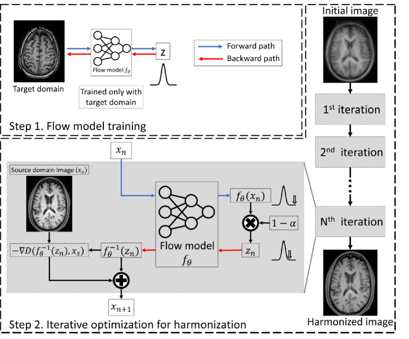
Figure 2: The BlindHarmony framework operates as follows: first, a flow model is trained solely on target domain data. Then, harmonization is performed iteratively on both latent variable and image domains using the flow model.

3.3 BlindHarmony optimization

In order to harmonize images from unknown domains, an unconditional flow model is trained on the target domain only. The prior distribution of the harmonized image $x$ can be parameterized as follows:

$$\log p_{X}\left(x\right)=\log\left(p_{Z}\left(z\right)\right)+\log\left|\det\frac{\partial{f_{\theta}\left(x\right)}}{\partial{x}}\right|.$$ (9)

If $z$ is a normal Gaussian, we can rewrite Equation 4 in the $z$-domain as follows:

$$\widehat{z_{h}}=\arg\min_{z}D\left(f_{\theta}^{-1}\left(z\right),x_{s}\right)-\alpha\log p_{Z}\left(z\right)$$ (10)

$$=\arg\min_{z}D\left(f_{\theta}^{-1}\left(z\right),x_{s}\right)+\alpha|z|^{2}.$$ (11)

The optimization process of Equation 11 requires the calculation of gradients of $f_{\theta}^{-1}\left(z\right)$, which can be computationally burdensome. To increase computational efficiency and reduce processing time, we simply omit the calculation of $\frac{\partial{f_{\theta}^{-1}\left(z\right)}}{\partial{z}}$. Instead, iterative optimization is performed in both the $z$- and $x$-domains, by leveraging the invertibility of normalizing flow. The algorithm alternates between a gradient descent of the distance measure $D\left(x,x_{s}\right)$ and a gradient descent of the prior term $|z|^{2}$.

In the latent vector domain $z$, $z$ is updated so that it does not deviate far from the center of the Gaussian:

$$z\rightarrow(1-\alpha)z.$$ (12)

In the image domain $x$, the gradient of $D\left(x,x_{s}\right)$ is measured and updated at each iteration as follows:

$$x\rightarrow x+\nabla_{x}[\beta_{1}NCC\left(x,x_{s}\right)-\beta_{2}\|MGx_{h}\|_{1}].$$ (13)

After $N$ iterations, the resultant image $x$ is a harmonized image $\widehat{x_{h}}$. The overall algorithm is formulated as Algorithm 1 (Fig. 2). The hyperparameters $\alpha$, $\beta_{1}$, and $\beta_{2}$ are found heuristically using grid search. The hyperparameters have been fixed as: $\alpha=0.001,\beta_{1}=1000,\beta_{2}=0.001,$ and $N=10$. The initial image $x_{0}$ is chosen to be the averaged image of the training data images.

Algorithm 1 BlindHarmony optimization

$x_{s}$: Source domain image

$\widehat{x_{h}}$: Harmonized image

$f_{\theta}$: Flow model trained on the target domain

$x_{0}$: Initial image

$\alpha$, $\beta_{1}$, $\beta_{2}$: Hyperparameters

$N$: The number of iteration

1:$x_{s}$, $x_{0}$, $\alpha$, $\beta_{1}$, $\beta_{2}$

2:for $n=0,1,\ldots,N-1$ do

3:     $x_{n+1}=f_{\theta}^{-1}\left(z_{n}\right)+\nabla_{x}[\beta_{1}NCC\left(x,x_{s}\right)-\beta_{2}\|MGx_{h}\|_{1}]_{x=f_{\theta}^{-1}\left(z_{n}\right)}$

4:     $z_{n+1}=\left(1-\alpha\right)f_{\theta}(x_{n+1})$

5:end for

6:$\widehat{x_{h}}=x_{N}$

4 Experiments

4.1 Dataset

T₁-weighted images in the OASIS3 dataset [24] were used to train and evaluate the proposed framework. The OASIS3 dataset consists of images scanned with different scanners. Images acquired with the Siemens TrioTim scanner were used as the target domain. For the source domain datasets, three datasets consisting of images acquired with different manufacturer models (Domain 1,2,3) and a dataset from a different scanner with the same manufacturer model (Domain 4) were used (see Supplementary material). All images were resampled to the same resolution of 1.2$\times$1.2$\times$1.2 mm³ and min-max normalized in a slice level.

4.2 Network training detail

In our experiments, we used the Neural Spline Flow (NSF) architecture with rational quadratic (RQ) spline coupling layers that was outlined by [14]. A Glow-like multiscale architecture was used, following NSF (Durkan et al., 2019) and Glow [21]. Each layer of the network contains 7 transformation steps, where each step consists of an actnorm layer, an invertible 1$\times$1 convolution an RQ spline coupling transform, and another 1$\times$1 convolution. The network consists of 4 layers, which results in a total of 28 coupling transformation steps. Also, 3 residual blocks and batch normalization layers are included in the subnetworks parameterizing the RQ splines. An Adam optimizer with an initial learning rate of 0.0005 and cosine annealing of the learning rate was used to iteratively optimize the parameters up to 20K steps. The sampled images are reported in the Supplementary material.

4.3 Simulated data evaluation

To evaluate the effectiveness of our proposed harmonization approach, we developed simulated data by applying three different image transformations: exponential transformation (Domain-Exp), log transformation (Domain-Log), and Gamma transformations with powers of 0.7 (Domain-Gamma0.7) to the target domain images. The target domain images were normalized with min-max normalization, then the three above transformations were applied. The min-max normalization was performed again on the transformed images to generate simulated source domain data. We applied BlindHarmony to the source domain.

To evaluate the performance of our proposed method, we compared it with the following methods: slice-wise histogram matching (HM), low-frequency replacing (SSIMH) [16], end-to-end U-net [35], and unsupervised CycleGAN [47]. We trained U-net_Exp, U-net_Log, U-net_Gamma0.7, CycleGAN_Exp, CycleGAN_Log, and CycleGAN_Gamma0.7 models for each domain mapping and used them for comparison (e.g., U-net_Exp was trained on Domain-Exp data).

	Source	Target	BlindHarmony	HM	SSIMH[16]	CycleGANExp[47]	U-netExp[35]
Domain-Exp
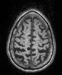
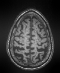
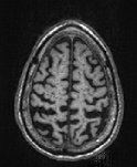
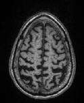
Domain-Log
Domain-Gamma0.7

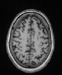
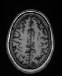
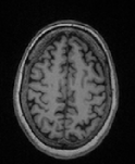
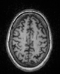
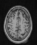
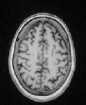
Figure 3: Example image of BlindHarmony application of simulated source domain images and comparison with other harmonization methods.

Figure 3 displays the results of our harmonization approach using BlindHarmony on each of the simulated source domain images (1st column), along with the target domain image (2nd column), and the other methods. A visual inspection of the results confirms the effectiveness of our approach in harmonizing images. On the other hand, CycleGAN and U-net fail to harmonize a source domain image when trained on another source domain dataset (e.g., U-net_Exp which was trained on Domain-Exp data while applying Domain-Gamma0.7 data). In contrast, BlindHarmony offers a more efficient and versatile solution by utilizing a single network for harmonization across diverse source domains.

			Domain-Exp		Domain-Log		Domain-Gamma0.7
	Unsupervised	Blind	PSNR($\uparrow$)	SSIM($\uparrow$)	PSNR($\uparrow$)	SSIM($\uparrow$)	PSNR($\uparrow$)	SSIM ($\uparrow$)
Source			22.6	0.952	21.4	0.958	21.6	0.955
BlindHarmony (Ours)	O	O	29.6	0.985	28.8	0.978	27.4	0.969
HM	O	O	26.5	0.961	26.5	0.961	26.5	0.961
SSIMH[16]	O	O	26.5	0.972	25.8	0.973	26.3	0.976
CycleGANExp[47]	O	X	32.6	0.993	23.0	0.951	23.0	0.948
CycleGANLog	O	X	22.8	0.943	35.5	0.996	34.5	0.995
CycleGANGamma0.7	O	X	22.1	0.932	35.6	0.996	35.6	0.996
U-netExp[35]	X	X	65.6	0.999	15.9	0.885	15.9	0.879
U-netLog	X	X	16.8	0.803	56.5	0.999	38.0	0.997
U-netGamma0.7	X	X	16.3	0.766	39.2	0.998	55.1	0.999

Table 1: The PSNR and SSIM values calculated between the harmonized image from the simulated source domain and the reference of the target domain image. The regions with signals were used as a mask.

Table 1 presents the results of our simulated data evaluation of the harmonization methods. We calculated the peak signal-to-noise ratio (PSNR) and structural similarity (SSIM) values using the target image as a reference. The table shows that our proposed BlindHarmony framework outperforms the source domain image, as evidenced by the improved PSNR and SSIM values. The averaged PSNR value improved from 21.9 dB for the source domain images to 28.6 dB for the BlindHarmony harmonized images. These results demonstrate the effectiveness of BlindHarmony in harmonizing images from different domains.

It is worth noting that U-net and CycleGAN outperformed BlindHarmony when they were trained separately for each source domain (e.g., U-net_Exp which was trained on Domain-Exp data while applying Domain-Exp data). However, BlindHarmony used only one network for all source domains, making it a practical solution for harmonizing images from multiple source domains.

	Source	Target	BlindHarmony	HM	SSIMH[16]	CycleGANeach[47]	U-neteach[35]
Domain 1
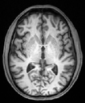
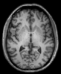
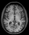
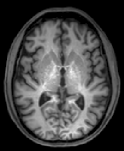
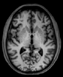
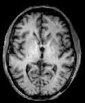
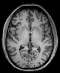
Domain 2
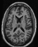
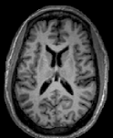
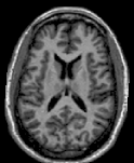
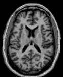
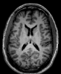
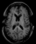
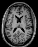
Domain 3
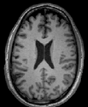
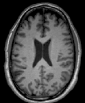
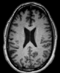
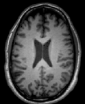
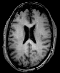
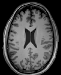
Domain 4

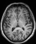
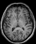
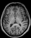
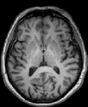
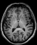
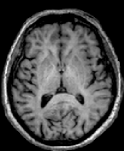
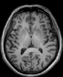
Figure 4: Example image of BlindHarmony application of real source domain images and comparison with other harmonization methods. CycleGAN and U-net results stand for the output of the network that was trained for each source domain.

4.4 Real-world data application

In addition to the simulation dataset, we also evaluated BlindHarmony on four real datasets from different scanners. Twenty traveling subjects from OASIS 3 [24] dataset who underwent multi-scanner scans were utilized in order to compare the results quantitatively. The image of each source domain is registered to the target domain image by using the FSL FLIRT [20] function. We compared the results with the other methods (U-Net and CycleGAN retrained for these datasets and conventional methods of volumetric HM and SSIMH). Figure 4 presents the results of harmonizing the source domain images (column 1) to the target domain images (column 2) using BlindHarmony (column 3). BlindHarmony effectively harmonized the images and reduced the inter-scanner variability, bringing them closer to the target domain images. The BlindHarmony also demonstrated superior harmonization performance not only to the conventional methods (SSIMH and HM) but also to the CycleGAN, which illustrates structural distortion.

			Domain1		Domain2		Domain3		Domain4
	Unsupervised	Blind	PSNR($\uparrow$)	SSIM($\uparrow$)	PSNR($\uparrow$)	SSIM($\uparrow$)	PSNR($\uparrow$)	SSIM($\uparrow$)	PSNR($\uparrow$)	SSIM ($\uparrow$)
Source			19.6	0.833	19.4	0.836	23.0	0.893	24.1	0.914
BlindHarmony (Ours)	O	O	20.2	0.840	20.8	0.850	23.0	0.892	24.6	0.912
HM	O	O	20.4	0.834	20.6	0.840	22.5	0.882	23.9	0.899
SSIMH[16]	O	O	20.4	0.831	20.4	0.833	22.0	0.882	22.6	0.896
CycleGANeach[47]	O	X	7.22	0.451	15.3	0.612	6.62	0.442	19.8	0.795
U-neteach[35]	X	X	25.0	0.919	23.4	0.890	25.1	0.925	25.6	0.920

Table 2: The quantitative results of application to real-world data. PSNR and SSIM values were calculated by using the target domain image as a reference. The case using BlindHarmony illustrated improved consistency to the target domain image. The regions with signals were used as a mask. CycleGAN_each and U-net_each stand for CycleGAN and U-net trained on each source domain (e.g., CycleGAN_each for Domain 1 application is trained on Domain 1 dataset).

The quantitative evaluation using PSNR and SSIM metrics demonstrated improvements in both PSNR and SSIM values compared to the source images (averaged PSNR: 21.5 dB to 22.2 dB). In particular, BlindHarmony has exhibited superior metric results compared to the HM, SSIMH, and CycleGAN algorithms.

The effect size of PSNR and SSIM improvement observed in this study is smaller than that in the simulated data study. This can be attributed to two key factors. Firstly, the domain gap between the source and target domains might be smaller than that in the simulated data, leading to a weaker harmonization effect. Secondly, the registration process between the source and target domains may not be perfectly aligned due to potential errors in registration and the time gap between separate scans. These factors may have led to a reduced effect of harmonization of effect of harmonization in the metric calculation.

	Source	Label	No harmonization	BlindHarmony	HM	SSIMH[16]	CycleGANeach[47]	U-neteach[35]
Domain 1
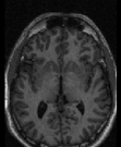
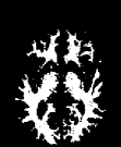
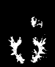
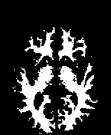
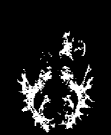
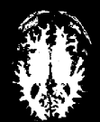
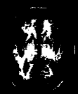
Domain 2
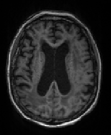
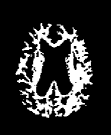
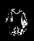
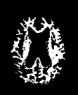
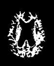
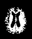
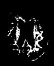
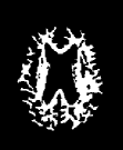
Domain 3
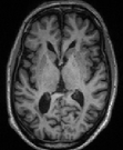
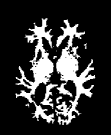
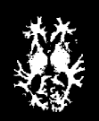
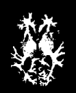
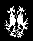
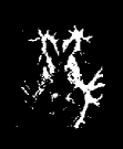
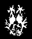
Domain 4

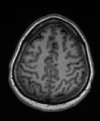
Figure 5: The results of the white matter segmentation network are presented, with each column representing the respective harmonization method applied to the input image.

IoU ($\uparrow$)	Domain 1	Domain 2	Domain 3	Domain 4
Source	0.912	0.845	0.947	0.938
BlindHarmony (Ours)	0.922	0.878	0.947	0.938
HM	0.863	0.854	0.911	0.894
SSIMH[16]	0.777	0.752	0.862	0.860
CycleGANeach[47]	0.306	0.408	0.394	0.299
U-neteach[35]	0.785	0.797	0.829	0.870

Table 3: The IOU values of the results of the segmentation network and label mask are reported. The case using BlindHarmony illustrated the best results when compared to other harmonization methods.

To further assess the impact of harmonization, we conducted an evaluation of the downstream task of white matter segmentation. For this task, a white matter segmentation network was trained to generate masks of white matter from given the T₁-weighted images. Notably, the network was solely trained on the target domain dataset, allowing us to measure harmonization performance through segmentation results with harmonized images as inputs. The white matter labels were generated using FSL FAST [45], and we adopted U-Net as the neural network architecture. Figure 5 shows the white matter segmentation results for each harmonization method. Remarkably, the outcomes demonstrate that BlindHarmony enhances segmentation performance, thus successfully harmonizing source domain images to the target domain more effectively than the other methods. For quantitative analysis, we computed the intersection over union (IoU) values between the predicted white matter masks and the label masks (Table 3). The IoU values were higher for BlindHarmony, further confirming its superior harmonization performance.

It is important to note that the dataset size used for U-net and CycleGAN training was smaller than that used for the flow model training due to the requirement of multiple domains for training. In addition, the U-net dataset size was even smaller due to the requirement of paired data. (e.g., Flow model training: 75,240 slices, Domain 1 CycleGAN training: 75,240 slices from the target domain and 17,400 slices from the source domain, Domain 1 U-net training: 5,100 slices; See Supplementary materials) Moreover, the construction of paired datasets required the registration of the source domain image to the target domain image using the FSL FLIRT function. Despite these efforts, there may still exist misregistration in the source domain-target domain pairs, which can negatively affect the training procedure and result in slightly blurred images produced by U-Net. These may be the reason for the inferior performance of CycleGAN and U-Net compared to their application for simulated source domains.

5 Discussion

In this work, we proposed BlindHarmony, a blind harmonization framework for harmonizing MR images from the source domain to the target domain. This framework does not require source domain data during training and can be applied to unseen source domain images. The flow-based prior distribution network is trained, and the harmonized images are optimized using a distance between the source domain image and the sampled image while using regularization based on the magnitude of the latent vector.

The fact that BlindHarmony does not require source domain data during training is beneficial when applying the neural network to an unknown dataset or a dataset that does not have sufficient data for training. For example, a deep learning-based API provider that utilizes a network trained on a certain dataset may not know the source domain information. In this scenario, our framework can be used as an excellent initial approach to harmonize data until sufficient data is collected for other methods.

In the real-world dataset evaluation involving the downstream task of white matter segmentation, BlindHarmony demonstrated superior performance compared to CycleGAN and U-Net, which were explicitly trained on specific source domains. While U-Net is good at image translation, it may miss fine structures. As for CycleGAN, it was originally designed to transfer style from source to target domains. In this harmonization case, the fine structure in MR images can also be considered as a style from the perspective of CycleGAN, leading to structural distortion in CycleGAN harmonization. Unlike image-to-image translation neural networks, BlindHarmony can enforce the structural information of the source domain images while harmonizing the images. This unique feature prevents the introduction of structural distortions and ensures more accurate and reliable harmonization results.

5.1 Limitations

BlindHarmony incorporates iterative optimization in both the image and latent vector domains. In order to reduce the computational burden of calculating the gradient of the network parameters, we have ignored the determinant term in Equation 9. Although this may compromise mathematical rigor, we believe that this simplification makes calculations easier and reduces processing time, making BlindHarmony more advantageous for practical use.

Gamma 1.5	PSNR($\uparrow$)
Source	22.6
BlindHarmony ($\beta_{1}=1000$)	25.7
BlindHarmony ($\beta_{1}=500$)	26.8
HM	26.5
SSIMH	26.3

Table 4: In the case of a simulated source domain with a Gamma transformation of 1.5, BlindHarmony exhibited inferior results when using predefined hyperparameters. However, fine-tuning the hyperparameters led to improvements in the harmonization outcomes.

Additionally, it should be noted that BlindHarmony may not be applicable in every domain. If the distance between two images defined in Equation 3 cannot capture the relationship between images of different domains (e.g., multi-contrast: T₁-weighted and T₂-weighted images), the optimization may fail and lead to poor results. For example, when applying an extreme contrast variation case such as simulated source domain data with Gamma transformation with a power of 1.5, BlindHarmony showed inferior results to conventional methods. (Table. 4) Therefore, it is important to carefully consider the suitability of BlindHarmony for different applications.

However, fine-tuning hyperparameters for each source domain may give improved results. As shown in Table 4, the PSNR value increased when we changed the hyperparameter $\beta_{1}$ from 1000 to 500. Tuning these hyperparameters for each source domain may give a successful application of our approach in various scenarios, providing a highly adaptable and versatile solution. Future work may include optimizing these parameters using a transfer learning approach, as demonstrated in [42].

6 Conclusion

In this study, we propose BlindHarmony, a flow-bassed blind harmonization method for MR images. Unlike other existing harmonization methods, our network is trained exclusively on the target domain dataset and can be applied to previously unseen domain images. The flow model is trained only on the target domain data, and the harmonized image is optimized to have a correlation with the source domain image while maintaining a high probability of the flow model. Both simulated and real-world datasets showed that our method achieves acceptable results. Our study demonstrates the feasibility of blind harmonization, providing an advantage in scenarios where access to source domain data is limited or unavailable.

Acknowledgements This work was supported by the funding agencies of the Republic of Korea (NRF- 2022R1A4A1030579, NRF-2021R1A2B5B03002783, 21NPSS-C163415-01, and IITP-2023-RS-2023-00256081), Radisen Co. Ltd. and INMC and IOER of Seoul National University.

References

- [1] Rameen Abdal, Peihao Zhu, Niloy J Mitra, and Peter Wonka. Styleflow: Attribute-conditioned exploration of stylegan-generated images using conditional continuous normalizing flows. ACM Transactions on Graphics (ToG), 40(3):1–21, 2021.
- [2] Abdelrahman Abdelhamed, Marcus A Brubaker, and Michael S Brown. Noise flow: Noise modeling with conditional normalizing flows. In Proceedings of the IEEE/CVF International Conference on Computer Vision, pages 3165–3173, 2019.
- [3] Zeynettin Akkus, Alfiia Galimzianova, Assaf Hoogi, Daniel L Rubin, and Bradley J Erickson. Deep learning for brain mri segmentation: state of the art and future directions. Journal of digital imaging, 30:449–459, 2017.
- [4] Muhammad Asim, Max Daniels, Oscar Leong, Ali Ahmed, and Paul Hand. Invertible generative models for inverse problems: mitigating representation error and dataset bias. In Proceeding of the International Conference on Machine Learning, pages 399–409, 2020.
- [5] Silvia Basaia, Federica Agosta, Luca Wagner, Elisa Canu, Giuseppe Magnani, Roberto Santangelo, Massimo Filippi, Alzheimer’s Disease Neuroimaging Initiative, et al. Automated classification of alzheimer’s disease and mild cognitive impairment using a single mri and deep neural networks. NeuroImage: Clinical, 21:101645, 2019.
- [6] Viola Biberacher, Paul Schmidt, Anisha Keshavan, Christine C Boucard, Ruthger Righart, Philipp Sämann, Christine Preibisch, Daniel Fröbel, Lilian Aly, Bernhard Hemmer, et al. Intra-and interscanner variability of magnetic resonance imaging based volumetry in multiple sclerosis. Neuroimage, 142:188–197, 2016.
- [7] Ashish Bora, Ajil Jalal, Eric Price, and Alexandros G Dimakis. Compressed sensing using generative models. In Proceeding of the International Conference on Machine Learning, pages 537–546, 2017.
- [8] Kristi A Clark, Roger P Woods, David A Rottenberg, Arthur W Toga, and John C Mazziotta. Impact of acquisition protocols and processing streams on tissue segmentation of t1 weighted mr images. NeuroImage, 29(1):185–202, 2006.
- [9] Blake E Dewey, Can Zhao, Jacob C Reinhold, Aaron Carass, Kathryn C Fitzgerald, Elias S Sotirchos, Shiv Saidha, Jiwon Oh, Dzung L Pham, Peter A Calabresi, et al. Deepharmony: A deep learning approach to contrast harmonization across scanner changes. Magnetic resonance imaging, 64:160–170, 2019.
- [10] Blake E Dewey, Lianrui Zuo, Aaron Carass, Yufan He, Yihao Liu, Ellen M Mowry, Scott Newsome, Jiwon Oh, Peter A Calabresi, and Jerry L Prince. A disentangled latent space for cross-site mri harmonization. In Proceedings of the Medical Image Computing and Computer Assisted Intervention, Part VII, pages 720–729. Springer, 2020.
- [11] Laurent Dinh, David Krueger, and Yoshua Bengio. Nice: Non-linear independent components estimation. arXiv preprint arXiv:1410.8516, 2014.
- [12] Laurent Dinh, Jascha Sohl-Dickstein, and Samy Bengio. Density estimation using real nvp. arXiv preprint arXiv:1605.08803, 2016.
- [13] Nicola K Dinsdale, Mark Jenkinson, and Ana IL Namburete. Deep learning-based unlearning of dataset bias for mri harmonisation and confound removal. NeuroImage, 228:117689, 2021.
- [14] Conor Durkan, Artur Bekasov, Iain Murray, and George Papamakarios. Neural spline flows. Advances in Neural Information Processing Systems, 32, 2019.
- [15] Jean-Philippe Fortin, Drew Parker, Birkan Tunç, Takanori Watanabe, Mark A Elliott, Kosha Ruparel, David R Roalf, Theodore D Satterthwaite, Ruben C Gur, Raquel E Gur, et al. Harmonization of multi-site diffusion tensor imaging data. Neuroimage, 161:149–170, 2017.
- [16] Hao Guan, Siyuan Liu, Weili Lin, Pew-Thian Yap, and Mingxia Liu. Fast image-level mri harmonization via spectrum analysis. In Proceedings of the MICCAI workshop on Machine Learning in Medical Imaging, pages 201–209. Springer, 2022.
- [17] Hao Guan, Yunbi Liu, Erkun Yang, Pew-Thian Yap, Dinggang Shen, and Mingxia Liu. Multi-site mri harmonization via attention-guided deep domain adaptation for brain disorder identification. Medical image analysis, 71:102076, 2021.
- [18] Kerstin Hammernik, Teresa Klatzer, Erich Kobler, Michael P Recht, Daniel K Sodickson, Thomas Pock, and Florian Knoll. Learning a variational network for reconstruction of accelerated mri data. Magnetic Resonance in Medicine, 79(6):3055–3071, 2018.
- [19] Ajil Jalal, Marius Arvinte, Giannis Daras, Eric Price, Alexandros G Dimakis, and Jon Tamir. Robust compressed sensing mri with deep generative priors. Advances in Neural Information Processing Systems, 34:14938–14954, 2021.
- [20] Mark Jenkinson, Peter Bannister, Michael Brady, and Stephen Smith. Improved optimization for the robust and accurate linear registration and motion correction of brain images. Neuroimage, 17(2):825–841, 2002.
- [21] Durk P Kingma and Prafulla Dhariwal. Glow: Generative flow with invertible 1x1 convolutions. Advances in Neural Information Processing Systems, 31, 2018.
- [22] Yilmaz Korkmaz, Salman UH Dar, Mahmut Yurt, Muzaffer Özbey, and Tolga Cukur. Unsupervised mri reconstruction via zero-shot learned adversarial transformers. IEEE Transactions on Medical Imaging, 41(7):1747–1763, 2022.
- [23] Sergey Korolev, Amir Safiullin, Mikhail Belyaev, and Yulia Dodonova. Residual and plain convolutional neural networks for 3d brain mri classification. In 2017 IEEE 14th international symposium on biomedical imaging, pages 835–838. IEEE, 2017.
- [24] Pamela J LaMontagne, Tammie LS Benzinger, John C Morris, Sarah Keefe, Russ Hornbeck, Chengjie Xiong, Elizabeth Grant, Jason Hassenstab, Krista Moulder, Andrei G Vlassenko, et al. Oasis-3: longitudinal neuroimaging, clinical, and cognitive dataset for normal aging and alzheimer disease. MedRxiv, pages 2019–12, 2019.
- [25] Yuan-kui Li, Yun-Hsuan Lien, and Yu-Shuen Wang. Style-structure disentangled features and normalizing flows for diverse icon colorization. In Proceedings of the IEEE/CVF Conference on Computer Vision and Pattern Recognition, pages 11244–11253, 2022.
- [26] Mengting Liu, Piyush Maiti, Sophia Thomopoulos, Alyssa Zhu, Yaqiong Chai, Hosung Kim, and Neda Jahanshad. Style transfer using generative adversarial networks for multi-site mri harmonization. In Proceedings of the Medical Image Computing and Computer Assisted Intervention, Part III 24, pages 313–322. Springer, 2021.
- [27] Andreas Lugmayr, Martin Danelljan, Luc Van Gool, and Radu Timofte. Srflow: Learning the super-resolution space with normalizing flow. In Proceedings of the European Conference on Computer Vision, Part V 16, pages 715–732. Springer, 2020.
- [28] Guanxiong Luo, Na Zhao, Wenhao Jiang, Edward S Hui, and Peng Cao. Mri reconstruction using deep bayesian estimation. Magnetic Resonance in Medicine, 84(4):2246–2261, 2020.
- [29] Hengameh Mirzaalian, Lipeng Ning, Peter Savadjiev, Ofer Pasternak, Sylvain Bouix, O Michailovich, Gerald Grant, Christine E Marx, Rajendra A Morey, Laura A Flashman, et al. Inter-site and inter-scanner diffusion mri data harmonization. NeuroImage, 135:311–323, 2016.
- [30] Gourav Modanwal, Adithya Vellal, Mateusz Buda, and Maciej A Mazurowski. Mri image harmonization using cycle-consistent generative adversarial network. In Medical Imaging 2020: Computer-Aided Diagnosis, volume 11314, pages 259–264. SPIE, 2020.
- [31] László G Nyúl and Jayaram K Udupa. On standardizing the mr image intensity scale. Magnetic Resonance in Medicine, 42(6):1072–1081, 1999.
- [32] László G Nyúl, Jayaram K Udupa, and Xuan Zhang. New variants of a method of mri scale standardization. IEEE transactions on medical imaging, 19(2):143–150, 2000.
- [33] George Papamakarios, Eric Nalisnick, Danilo Jimenez Rezende, Shakir Mohamed, and Balaji Lakshminarayanan. Normalizing flows for probabilistic modeling and inference. The Journal of Machine Learning Research, 22(1):2617–2680, 2021.
- [34] Raymond Pomponio, Guray Erus, Mohamad Habes, Jimit Doshi, Dhivya Srinivasan, Elizabeth Mamourian, Vishnu Bashyam, Ilya M Nasrallah, Theodore D Satterthwaite, Yong Fan, et al. Harmonization of large mri datasets for the analysis of brain imaging patterns throughout the lifespan. NeuroImage, 208:116450, 2020.
- [35] Olaf Ronneberger, Philipp Fischer, and Thomas Brox. U-net: Convolutional networks for biomedical image segmentation. In Proceedings of the Medical Image Computing and Computer Assisted Intervention, Part III 18, pages 234–241. Springer, 2015.
- [36] Christian Salvatore, Antonio Cerasa, Isabella Castiglioni, F Gallivanone, A Augimeri, M Lopez, G Arabia, M Morelli, MC Gilardi, and A Quattrone. Machine learning on brain mri data for differential diagnosis of parkinson’s disease and progressive supranuclear palsy. Journal of neuroscience methods, 222:230–237, 2014.
- [37] Russell T Shinohara, Jiwon Oh, Govind Nair, Peter A Calabresi, Christos Davatzikos, Jimit Doshi, Roland G Henry, Gloria Kim, Kristin A Linn, Nico Papinutto, et al. Volumetric analysis from a harmonized multisite brain mri study of a single subject with multiple sclerosis. American Journal of Neuroradiology, 38(8):1501–1509, 2017.
- [38] Russell T Shinohara, Elizabeth M Sweeney, Jeff Goldsmith, Navid Shiee, Farrah J Mateen, Peter A Calabresi, Samson Jarso, Dzung L Pham, Daniel S Reich, Ciprian M Crainiceanu, et al. Statistical normalization techniques for magnetic resonance imaging. NeuroImage: Clinical, 6:9–19, 2014.
- [39] Ki-Ung Song, Dongseok Shim, Kang-wook Kim, Jae-young Lee, and Younggeun Kim. Fs-ncsr: Increasing diversity of the super-resolution space via frequency separation and noise-conditioned normalizing flow. In Proceeding of the IEEE/CVF Conference on Computer Vision and Pattern Recognition Workshops, pages 967–976. IEEE, 2022.
- [40] Dmitry Ulyanov, Andrea Vedaldi, and Victor Lempitsky. Deep image prior. In Proceedings of the IEEE/CVF Conference on Computer Vision and Pattern Recognition, pages 9446–9454, 2018.
- [41] Ben Usman, Avneesh Sud, Nick Dufour, and Kate Saenko. Log-likelihood ratio minimizing flows: Towards robust and quantifiable neural distribution alignment. Advances in Neural Information Processing Systems, 33:21118–21129, 2020.
- [42] Xinyi Wei, Hans van Gorp, Lizeth Gonzalez-Carabarin, Daniel Freedman, Yonina C Eldar, and Ruud JG van Sloun. Deep unfolding with normalizing flow priors for inverse problems. IEEE Transactions on Signal Processing, 70:2962–2971, 2022.
- [43] Jay Whang, Qi Lei, and Alex Dimakis. Solving inverse problems with a flow-based noise model. In Proceeding of the International Conference on Machine Learning, pages 11146–11157, 2021.
- [44] Jaeyeon Yoon, Enhao Gong, Itthi Chatnuntawech, Berkin Bilgic, Jingu Lee, Woojin Jung, Jingyu Ko, Hosan Jung, Kawin Setsompop, Greg Zaharchuk, et al. Quantitative susceptibility mapping using deep neural network: Qsmnet. Neuroimage, 179:199–206, 2018.
- [45] Yongyue Zhang, Michael Brady, and Stephen Smith. Segmentation of brain mr images through a hidden markov random field model and the expectation-maximization algorithm. IEEE transactions on medical imaging, 20(1):45–57, 2001.
- [46] Xiaomei Zhao, Yihong Wu, Guidong Song, Zhenye Li, Yazhuo Zhang, and Yong Fan. A deep learning model integrating fcnns and crfs for brain tumor segmentation. Medical image analysis, 43:98–111, 2018.
- [47] Jun-Yan Zhu, Taesung Park, Phillip Isola, and Alexei A Efros. Unpaired image-to-image translation using cycle-consistent adversarial networks. In Proceedings of the IEEE/CVF International Conference on Computer Vision, pages 2223–2232, 2017.
- [48] Lianrui Zuo, Blake E Dewey, Yihao Liu, Yufan He, Scott D Newsome, Ellen M Mowry, Susan M Resnick, Jerry L Prince, and Aaron Carass. Unsupervised mr harmonization by learning disentangled representations using information bottleneck theory. NeuroImage, 243:118569, 2021.