FedMR: Federated Learning via Model Recombination

Abstract

Although Federated Learning (FL) enables global model training across clients without compromising their raw data, existing Federated Averaging (FedAvg)-based methods suffer from the problem of low inference performance, especially for unevenly distributed data among clients. This is mainly because i) FedAvg initializes client models with the same global models, which makes the local training hard to escape from the local search for optimal solutions; and ii) by averaging model parameters in a coarse manner, FedAvg eclipses the individual characteristics of local models. To address such issues that strongly limit the inference capability of FL, we propose a novel and effective FL paradigm named FedMR (Federated Model Recombination). Unlike conventional FedAvg-based methods, the cloud server of FedMR shuffles each layer of collected local models and recombines them to achieve new models for local training on clients. Due to the diversified initialization models for clients coupled with fine-grained model recombination, FedMR can converge to a well-generalized global model for all the clients, leading to a superior inference performance. Experimental results show that, compared with state-of-the-art FL methods, FedMR can significantly improve inference accuracy in a quicker manner without exposing client privacy.

1 Introduction

Federated Learning (FL) [1] has been widely acknowledged as a promising means to design large-scale distributed Artificial Intelligence (AI) applications, e.g., Artificial Intelligence of Things (AIoT) systems [2, 3], healthcare systems [4, 5], and recommender systems [6]. Unlike conventional Deep Learning (DL) methods, the cloud-client architecture based FL supports the collaborative training of a global DL model among clients without compromising their data privacy [7, 8, 9]. In each FL training round, the cloud server first dispatches an intermediate model to its selected clients for local training and then gathers the corresponding gradients of trained models from clients for aggregation. In this way, only clients can touch their own raw data, thus client privacy is guaranteed. Although FL enables effective collaborative training towards a global optimal model for all the clients, when dealing with unevenly distributed data on clients, existing mainstream FL methods suffer from the problem of “weight divergence” [10]. Especially when the data on clients are non-IID (Identically and Independently Distributed) [11, 12], the optimal directions of local models on clients and the aggregated global model on the cloud server are significantly inconsistent, resulting in serious inference performance degradation of the global model.

Aiming to mitigate such a phenomenon and improve FL performance in non-IID scenarios, various FL methods have been studied, e.g., client grouping-based methods [13], global control variable-based methods [14, 15, 16], and Knowledge Distillation (KD)-based methods[17, 18]. The basic ideas of these solutions are to guide the local training on clients [14, 15] or adjust parameter weights for model aggregation [13, 17, 18]. Although these methods are promising to alleviate the impact of data heterogeneity, most of them adopt the well-known Federated Averaging (FedAvg)-based aggregation, which may potentially reduce the generalization performance. This is mainly because FedAvg operations only average the parameters of collected local models in a coarse manner, where the specific characteristics of client data learned by local models are almost neglected. As a result, an intermediate global model based on simple statistical averaging cannot accurately reflect both the individual efforts and potential of local models in searching for optimal global models.

Besides the average operation, another bottleneck of FedAvg is the uniform global model for local training initialization, which further degrades the overall generalization performance of derived global models. Some recent research on model training indicates that, from the perspective of the loss landscapes of DL models, optimal solutions with the best generalization performance often lie in flat valleys, while inferior ones are always located in sharp ravines [19, 20, 21, 22]. According to such a finding, the generalization performance of FedAvg is hard to be guaranteed. This is because FedAvg initializes the local training with the same global models, which limits the diversity of local searching. This will inevitably result in the notorious stuck-at-local-search problem during the local training, leading to the problems of both an extremely long convergence time and low inference performance.

To address the above issues, this paper proposes a novel FL paradigm called FedMR (Federated Model Recombination), which can effectively help the training of local models escape from local minima, while the individual characteristics of local models are still maintained. Unlike FedAvg that aggregates all the collected local models in each FL training round, FedMR randomly shuffles the parameters of different local models within the same layers, and recombines them to form new local models. In this way, FedMR can not only keep individual characteristics of local models at layer-level, but also derive diversified models that can effectively escape from local optimal solutions for the local training of clients. The main contributions of this paper can be summarized as follows:

• We propose to use our designed fine-grained model recombination method to replace the traditional FedAvg-based model aggregation, and prove its convergence, with the aim of improving FL inference performance.

• We introduce an effective two-stage training scheme for FedMR, which combines the merits of both model recombination and aggregation to accelerate the overall FL training process.

• We conduct extensive experiments on various models and datasets to show both the effectiveness and compatibility of FedMR.

2 Related Work

To address the problem of uneven data distributions, exiting solutions can be mainly classified into three categories, i.e., client grouping-based methods, global control variable-based methods, and knowledge distillation-based methods. The device grouping-based methods group and select clients for aggregation based on the data similarity between clients. For example, FedCluster [23] divides clients into multiple clusters and performs multiple cycles of meta-update to boost the overall FL convergence. Based on either sample size or model similarity, CluSamp [24] groups clients to achieve a better client representativity and a reduced variance of client stochastic aggregation parameters in FL. By modifying the penalty terms of loss functions during FL training, the global control variable-based methods can be used to smooth the FL convergence process. For example, FedProx [16] regularizes local loss functions with the squared distance between local models and the global model to stabilize the model convergence. Similarly, SCAFFOLD [14] uses global control variables to correct the “client-drift” problem in the local training process. Knowledge Distillation (KD)-based methods adopt soft targets generated by the “teacher model” to guide the training of “student models”. For example, by leveraging a proxy dataset, Zhu et al. [18] proposed a data-free knowledge distillation method named FedGen to address the heterogeneous FL problem using a built-in generator. With ensemble distillation, FedDF [17] accelerates the FL training by training the global model through unlabeled data on the outputs of local models.

Although the above methods can optimize FL performance from different perspectives, since conducts coarse-grained model aggregation, the inference capabilities of local models are still strongly restricted. Furthermore, most of them cannot avoid non-negligible communication and computation overheads or the risk of data privacy exposure. To the best of our knowledge, FedMR is the first attempt that uses model recombination and different models for fine-grained FL. Since FedMR considers the specific characteristics and efforts of local models, it can further mitigate the weight divergence problem, thus achieving better inference performance than state-of-the-art FL methods.

3 Motivation

Comparison between FedAvg and Independent Training. Figure 1 illustrates the FL training processes on the same loss landscape using FedAvg and Independent training (Indep), respectively, where the server of Indep just shuffles the received local models and then randomly dispatches them to clients without aggregation. In each subfigure, the local optima are located within the areas surrounded by red solid lines. Note that, since the upper surrounded area is flatter than the lower surrounded area in the loss landscape, the solutions within it will exhibit better generalization.

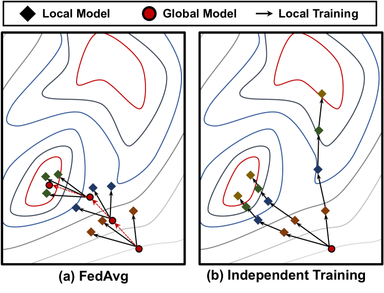
Figure 1: Training processes on the same loss landscape.

As shown in Figure 1(a), along with the training process, the aggregated global models denoted by red circles gradually move toward the lower sharp area with inferior solutions, though the optimization of some local models heads toward the upper surrounded area with better solutions. The reason for such biased training is mainly because the local training starts from the same global model in each FL round. As an alternative, due to the lack of aggregation operation, the local models of Indep may converge in different directions as shown in Figure 1(b). In this case, even if some local training in Idep achieves a better solution than the one obtained by FedAvg, due to diversified optimization directions of local models, such an important finding can be eclipsed by the results of other local models. Clearly, there is a lack of mechanisms for Indep that can guide the overall training toward such superior solutions.

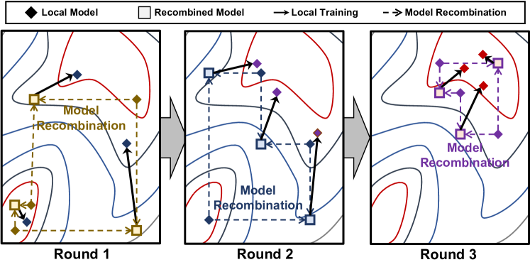
Figure 2: An example of model recombination.

Intuition of Model Recombination. Based on the Indep training results shown in Figure 1(b), Figure 2 illustrates the intuition of our model recombination method, where the FL training starts from the three local models (denoted by yellow diamonds in round 1) obtained in figure 1(b). Note that, at the beginning of round 1, two of the three local models are located in the sharp ravine. In other words, without model recombination, the training of such two local models may get stuck in the lower surrounded area. However, due to the weight adjustment by shuffling the layers among local models, we can find that the three recombined models (denoted by yellow squares) are sparsely scattered in the loss landscape, which enables the local training escape from local optima. According to [25, 26], a small perturbation of the model weights can make it easier for local training to jump out of sharp ravines rather than flat valleys. In other words, the recombined models are more likely to converge toward flat valleys along the local training. For example, in the end of round 3, we can find that all three local models are located in the upper surrounded area, where their aggregated model has better generalization performance than the one achieved in Figure 1(a).

4 FedMR Approach

4.1 Overview of FedMR

Figure 3(a) presents the framework and workflow of FedMR, where each training round involves three specific steps as follows:

Step 1 (Model Dispatching): The cloud server dispatches $K$ recombined models to $K$ selected clients according to their indices, where $K$ is the number of activated clients, which participate in each round of FL training. Note that, unlike FedAvg-based FL methods, in FedMR different clients will receive different models for the local training purpose.

Step 2 (Model Upload): Once the local training is finished, a client needs to upload the parameters of its trained local model to the cloud server.

Step 3 (Model Recombination): The cloud server decomposes received local models into multiple layers individually in the same manner and then conducts the random shuffling of the same layers among different local models. Finally, by concatenating layers from different sources in order, a new local model can be reconstructed. Note that any decomposed layer of the uploaded model will eventually be used by one and only one of the recombined models.

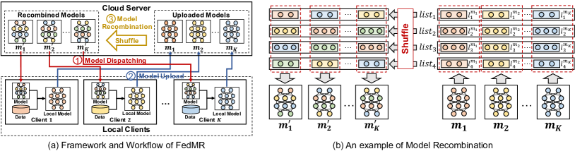
Figure 3: Our FedMR approach

Algorithm 1 Implementation of FedMR

Input: i) $rnd$, # of training rounds;
ii) $S_{c}$, the set of clients;
iii) $K$, # of clients participating in each FL round.
Output: $w^{glb}$, the parameters of trained global model.
FedMR($rnd$,$S_{dev}$,$K$)

1:  $L_{m}\leftarrow[w^{1}_{1},w^{2}_{1},...,w^{K}_{1}]\ \ \$ // initialize model list  

2:  for $r$ = 1, …, $rnd$ do

3:     $L_{r}\leftarrow$ Random select $K$ clients from $S_{c}$  /*parallel for block*/

4:     for $i$ = 1, …, $K$ do

5:        $v_{r+1}^{i}\leftarrow$ClientUpdate$(L_{m}[i],L_{r}[i])$ 

6:        $L_{m}[i]\leftarrow v_{r+1}^{i}$ 

7:     end for

8:     $[w_{r+1}^{1},w_{r+1}^{2},...,w_{r+1}^{K}]\leftarrow$ModelRcombine$(L_{m})$ 

9:     $L_{m}\leftarrow[w_{r+1}^{1},w_{r+1}^{2},...,w_{r+1}^{K}]$ 

10:  end for

11:  $w^{glb}\leftarrow\frac{1}{K}\sum_{i=1}^{K}w_{rnd+1}^{i}$  

12:  return $w^{glb}$ 

4.2 Implementation of FedMR

Algorithm 1 details the implementation of FedMR. Line 1 initializes the model list $L_{m}$, which includes $K$ initial models. Lines 2-10 performs $rnd$ rounds of FedMR training. In each round, Line 3 selects $K$ random clients to participate the model training and creates a client list $L_{r}$. Lines 4-7 conduct the local training on clients in parallel, where Line 5 applies the local model $L_{m}[i]$ on client $L_{r}[i]$ for local training by using the function ClientUpdate, and Line 6 achieves a new local model after the local training. After the cloud server receives all the $K$ local models, Line 8 uses the function ModelRcombine to recombine local models and generate $K$ new local models, which are saved in $L_{m}$ as shown in Line 9. Finally, Lines 11-12 will report an optimal global model that is generated based on $L_{m}$. Note that the global model will be dispatched by the cloud server to all the clients for the purpose of inference rather than local training. The following parts will detail the key components of FedMR. Since FedMR cannot adapt to the secure aggregation mechanism [27], to further protect privacy, we present an extended secure recombination mechanism in Appendix B, which enables the exchange of partial layers among clients before local training or model uploading to ensure that the cloud server cannot directly obtain the gradients of each local model.

Local Model Training. Unlike conventional FL methods that conduct local training on clients starting from the same aggregated model, in each training round FedMR uses different recombined models (i.e., $K$ models in the model list $L_{m}$) for the local training purpose. Note that, in the whole training phase, FedMR only uses $K$ ($K\leq|S_{c}|$) models, since there are only $K$ devices activated in each training round. Let $w^{c}_{r}$ be the parameters of some model that is dispatched to the $c^{th}$ client in the $r^{th}$ training round. In the $r^{th}$ training round, we dispatch the $i^{th}$ model in $L_{m}$ to its corresponding client using $w^{L_{r}[i]}_{r}=L_{m}[i]$. Based on the recombined model, FedMR conducts the local training on client $L_{r}[i]$ as follows:

$$\footnotesize v^{L_{r}[i]}_{r+1}=w^{L_{r}[i]}_{r}-\eta\nabla f_{L_{r}[i]}(w^{L_{r}[i]}_{r}),\ s.t.,\ f_{L_{r}[i]}(w^{L_{r}[i]}_{r})=\frac{1}{|D_{L_{r}[i]}|}\sum_{j=1}^{|D_{L_{r}[i]}|}\ell(w^{L_{r}[i]}_{r};x_{j};y_{j}),$$

where $v^{L_{r}[i]}_{r}$ indicates parameters of the trained local model, $D_{L_{r}[i]}$ denotes the dataset of client $L_{r}[i]$, $\eta$ is the learning rate, $\ell(\cdot)$ is the loss function, $x_{j}$ is the $j^{th}$ sample in $D_{L_{r}[i]}$, and $y_{j}$ is the label of $x_{j}$. Once the local training is finished, the client needs to upload the parameters of its trained local model to the cloud server by updating $L_{m}$ using $L_{m}[i]=v^{L_{r}[i]}_{r+1}$. Note that, similar to traditional FL methods, in each training round FedMR needs to transmit the parameters of $2K$ models between the cloud server and its selected clients.

Model Recombination. Typically, a DL model consists of multiple layers, e.g., convolutional layers, pooling layers, and Fully Connected (FC) layers. To simplify the description of our model recombination method, we do not explicitly present the layer types here. Let $w_{x}=\{l_{1}^{x},l_{2}^{x},...,l_{n}^{x}\}$ be the parameters of model $x$, where $l_{i}^{x}$ ($i\in[n]$) denotes the parameters of the $i^{th}$ layer of model $x$.

In each FL round, FedMR needs to conduct the model recombination base on $L_{m}$ to obtain new models for the local training. Figure 3(b) shows an example of model recombination based on the shuffling of model layers. When receiving all the trained local models (i.e., $m_{1}$, $m_{2}$, …, $m_{K}$) from clients, firstly the cloud server needs to decouple the layers of these models individually. For example, the model $m_{1}$ can be decomposed into four layers. Assuming that the local models are with an architecture of $w$, to enable the recombination, FedMR then constructs $n$ lists, where the $k^{th}$ ($k\in[n]$) list contains all the $k^{th}$ layers of the models in $L_{m}$. As an example shown in Figure 3(b), FedMR constructs four lists (i.e., $list_{1}$-$list_{4}$) for the $K$ models (i.e., $m_{1}$-$m_{K}$), where each list consists of $K$ elements (i.e., $K$ layers with the same index). After shuffling each list, FedMR generates $|L_{m}|$ recombined models based on shuffled results. For example, the top three layers of the recombined model $m^{\prime}_{1}$ come from the models $m_{1}$, $m_{2}$ and $m_{K}$, respectively.

4.3 Two-Stage Training Scheme for FedMR

Although FedMR enables finer FL training, when starting from blank models, FedMR converges more slowly than traditional FL methods at the beginning. This is mainly because, due to the low matching degree between layers in the recombined models, the model recombination operation in this stage requires more local training time to re-construct the new dependencies between layers. To accelerate the overall convergence, we propose a two-stage training scheme for FedMR, consisting of both the aggregation-based pre-training stage and model recombination stage. In the first stage, we train the local models coarsely using the FedAvg-based aggregation, which can quickly form a pre-trained global model. In the second stage, starting from the pre-trained models, FedMR dispatches recombined models to clients for local training. Due to the synergy of both FL paradigms, the overall FedMR training time can be reduced.

4.4 Convergence Analysis

Based on the same assumptions [28] as follows posed on the loss functions of local clients in FedAvg, this subsection conducts the convergence analysis for FedMR.

Assumption 4.1.

For $i\in\{1,2,\cdots,K\}$, $f_{i}$ is L-smooth satisfying $||\nabla f_{i}(x)-\nabla f_{i}(y)||\leq\frac{L}{2}||x-y||$.

Assumption 4.2.

For $i\in\{1,2,\cdots,K\}$, $f_{i}$ is $\mu$-strongly convex satisfying $||\nabla f_{i}(x)-\nabla f_{i}(y)||\geq\frac{\mu}{2}||x-y||$, where $\mu\geq 0$.

Assumption 4.3.

The variance of stochastic gradients is upper bounded by $\theta^{2}$ and the expectation of squared norm of stochastic gradients is upper bounded by $G^{2}$, i.e., $\mathbb{E}||\nabla f_{k}(w;\xi)-\nabla f_{k}(w)||^{2}\leq\theta^{2}$, $\mathbb{E}||\nabla f_{k}(w;\xi)||^{2}\leq G^{2}$, where $\xi$ is a data batch of the $k^{th}$ client in the $t^{th}$ FL round.

Based on the implementation of function ModelRecombine($\cdot$), we can derive the following two lemmas for the model recombination operation:

Lemma 4.4.

Assume that in FedMR there are $K$ clients participating in every FL training round. Let $\{v^{1}_{r},v^{2}_{r},..,v^{K}_{r}\}$ and $\{w^{1}_{r},w^{2}_{r},..,w^{K}_{r}\}$ be the set of trained local model weights and the set of recombined model weights generated in the $(r-1)^{th}$ round, respectively. Assume $x$ is a vector with the same size as that of $v_{r}^{k}$. We have

$$\scriptsize\sum_{k=1}^{K}v_{r}^{k}=\sum_{k=1}^{K}w_{r}^{k},\ and\ \sum_{k=1}^{K}||v_{r}^{k}-x||^{2}=\sum_{k=1}^{K}||w_{r}^{k}-x||^{2}.$$

We prove Theorem 1 based on Lemmas 4.4. Please refer to Appendix A for the proof.

Theorem 1.

(Convergence of FedMR) Let Assumption 4.1, 4.2, and 4.3 hold. Assume that $E$ is the number of SGD iterations conducted within one FL round, model recombination is conducted at the end of each FL round, and the whole training terminates after $n$ FL rounds. Let $T=n\times E$ be the total number of SGD iterations conducted so far, and $\eta_{k}=\frac{2}{\mu(T+\gamma)}$ be the learning rate. We can have

$$\scriptsize\begin{split}\mathbb{E}[f(\overline{w}_{T})]-f^{\star}\leq\frac{L}{2\mu(T+\gamma)}[\frac{4B}{\mu}+\frac{\mu(\gamma+1)}{2}\Delta_{1}]\end{split},$$

where $B=10L\Gamma+4(E-1)^{2}G^{2},\overline{w}_{T}=\sum_{k}=1^{K}{w^{k}_{T}}.$

Theorem 1 indicates that the difference between the current loss $f(\overline{w}_{T})$ and the optimal loss $f^{\star}$ is inversely related to $t$. From Theorem 1, we can find that the convergence rate of FedMR is similar to that of FedAvg, which has been analyzed in [28].

5 Experimental Results

5.1 Experimental Settings

To evaluate the effectiveness of FedMR, we implemented FedMR on top of a cloud-based architecture. Since it is impractical to allow all the clients to get involved in the training processes simultaneously, we assumed that there are only 10% of clients participating in the local training in each FL round. To enable fair comparison, all the investigated FL methods including FedMR set SGD optimizer with a learning rate of 0.01 and a momentum of 0.9. For each client, we set the batch size of local training to 50, and performed five epochs for each local training. All the experimental results were obtained from an Ubuntu workstation with Intel i9 CPU, 32GB memory, and NVIDIA RTX 3080 GPU.

Baseline Method Settings. We compared the test accuracy of FedMR with six baseline methods, i.e., FedAvg [1], FedProx [16], SCAFFOLD [14], MOON [29], FedGen [18], and CluSamp [24]. Here, FedAvg is the most classical FL method, while the other five methods are the state-of-the-art (SOTA) representatives of the three kinds of FL optimization methods introduced in the related work section. Specifically, FedProx, SCAFFOLD, and MOON are global control variable-based methods, FedGen is a KD-based approach, and CluSamp is a device grouping-based method. For FedProx, we used a hyper-parameter $\mu$ to control the weight of its proximal term, where the best values of $\mu$ for CIFAR-10, CIFAR-100, and FEMNIST are 0.01, 0.001, and 0.1, respectively. For FedGen, we adopted the same server settings presented in [18]. For CluSamp, the clients were clustered based on the model gradient similarity as described in [24].

Dataset Settings. We investigated the performance of our approach on three well-known datasets, i.e., CIFAR-10, CIFAR-100 [30], and FMNIST [31]. We adopted the Dirichlet distribution [32] to control the heterogeneity of client data for both CIFAR-10 and CIFAR-100. Here, the notation $Dir(\alpha)$ indicates a different Dirichlet distribution controlled by $\alpha$, where a smaller $\alpha$ means higher data heterogeneity of clients. Note that, different from datasets CIFAR-10 and CIFAR-100, the raw data of FEMNIST are naturally non-IID distributed. Since FEMNIST takes various kinds of data heterogeneity into account, we did not apply the Dirichlet distribution on FEMNIST. For both CIFAR-10 and CIFAR-100, we assumed that there are 100 clients in total participating in FL. For FEMNIST, we only considered one non-IID scenario involving 180 clients, where each client hosts more than 100 local data samples.

Model Settings. To demonstrate the pervasiveness of our approach, we developed different FedMR implementations based on three different models (i.e., CNN, ResNet-20, VGG-16). Here, we obtained the CNN model from [1], which consists of two convolutional layers and two FC layers. When conducting FedMR based on the CNN model, we directly applied the model recombination for local training on it without pre-training a global model, since CNN here only has four layers. We obtained both ResNet-20 and VGG-16 models from Torchvision [33]. · When performing FedMR based on ResNet-20 and VGG-16, due to the deep structure of both models, we adopted the two-stage training scheme, where the first stage lasts for 100 rounds to obtain a pre-trained global model.

5.2 Validation for Intuitions

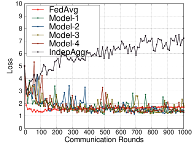
(a) Test Loss

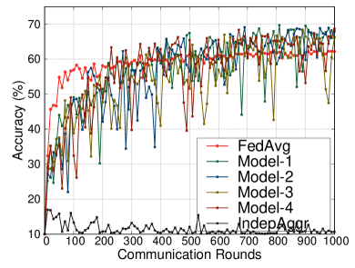
(b) Accuracy

Figure 4: FedAvg vs. Indep.

Independent Training. Based on the experimental settings presented in Section 5.1, we conducted the experiments to evaluate the effectiveness of each local model in Indep. The FL training is based on the ResNet-20 model and dataset CIFAR-10, where we set $\alpha=0.5$ for non-IID scenarios. Figures 4 compares Indep with FedAvg from the perspectives of both test loss and inference accuracy. Due to the space limitation, for Indep here we only present the results of its four random local models (denoted by Model-1, Model-2, Model-3, and Model-4). To enable a fair comparison with FedAvg, although there is no aggregated global model in Indep, we considered the aggregated model of all its local models for each FL round, whose results are indicated by the notion “IndepAggr”. From Figure 4, we can find that all the local models in Indep can achieve both higher accuracy and lower loss than those of FedAvg, though their loss and accuracy curves fluctuate more sharply. Moreover, IndepAggr exhibits much worse performance than the other references. This is mainly because, according to the definition of Indep, each local model needs to traverse multiple clients along with the FL training processes, where the optimization directions of client models differ in the corresponding loss landscape.

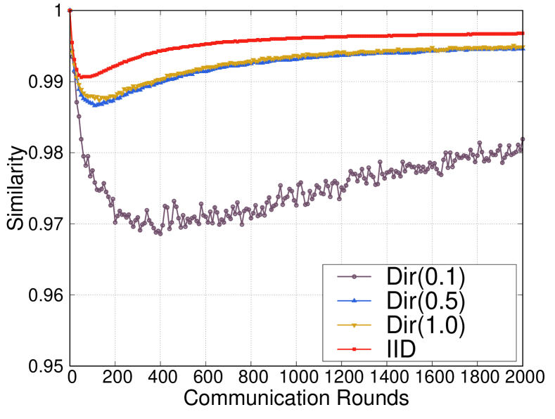
Figure 5: Cosine similarity of local models in FedMR.

Model Recombination. To validate the intuition about the impacts of model recombination as presented in Section 3, we conducted three experiments on CIFAR-10 dataset using ResNet-20 model. Our goal is to figure out the following three questions: i) by using model recombination, can all the models eventually have the same optimization direction; ii) compared with FedAvg, can the global model of FedMR eventually converge into a more flat solution; and iii) can the global model of FedMR eventually converge to a more generalized solution?

Figure 5 presents the average cosine similarity between all the intermediate models, taking four different client data distributions into account. We can observe that the model similarity decreases first and then gradually increases in all the investigated IID and non-IID scenarios. This is mainly because, due to the nature of Stochastic Gradient Descent (SGD) mechanism and the data heterogeneity among clients, all local models are optimized toward different directions at the beginning of training. However, as the training progresses, the majority of local models will be located in the same flat valleys, leading to similar optimization directions for local models. These results are consistent with our intuition as shown in Figure 2.

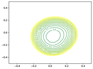
(a) FedAvg w/ $\alpha=0.1$

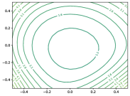
(b) FedMR w/ $\alpha=0.1$

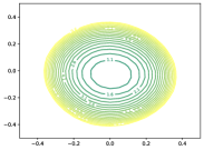
(c) FedAvg w/ $\alpha=1.0$

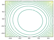
(d) FedMR w/ $\alpha=1.0$

Figure 6: Comparison of loss landscapes with different FL and client data settings.

Figure 6 compares the loss landscapes of final global models obtained by FedAvg and FedMR with different client data settings, respectively. We can find that, compared with FedMR counterparts, the global models trained by FedAvg are located in sharper solutions, indicating the generalization superiority of final global models achieved by FedMR.

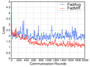
(a) $\alpha=0.1$

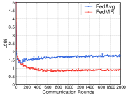
(b) $\alpha=0.5$

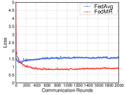
(c) $\alpha=1.0$

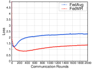
(d) IID

Figure 7: Comparison of test losses of FedAvg and FedMR with different client data settings.

Figure 7 compares the test losses for the global models of FedAvg and FedMR (without using two-stage training) within different IID and non-IID scenarios. Note that here the global models of FedMR are only for the purpose of fair comparison rather than local model initialization. We can observe that, due to the superiority in generalization, the models trained by FedMR outperform those by FedAvg for all the four cases.

5.3 Performance Comparison

We compared the performance of our FedMR approach with six SOTA baselines. For datasets CIFAR-10 and CIFAR-100, we considered both IID and non-IID scenarios (with $\alpha=0.1,0.5,1.0$, respectively). For dataset FEMNIST, we considered its original non-IID settings [31]. We also present the analysis of the comparison of computing and communication overhead in Appendix C.1.

Comparison of Test Accuracy        Table 1 compares FedMR with the SOTA FL methods considering both non-IID and IID scenarios based on three different DL models. The first two columns denote the model type and dataset type, respectively. Note that to enable fair comparison, we cluster the test accuracy results generated by the FL methods based on the same type of local models. The third column shows different distribution settings for client data, indicating the data heterogeneity of clients. The fourth column has seven sub-columns, which present the test accuracy information together with its standard deviation for all the investigated FL methods, respectively.

Table 1: Test accuracy comparison for both non-IID and IID scenarios using three DL models

Model	Datas.	Heter.	Test Accuracy (%)
		Set.	FedAvg	FedProx	SCAFFOLD	MOON	FedGen	CluSamp	FedMR
CNN	CF10	$0.1$	$46.12\pm 2.35$	$47.17\pm 1.65$	$49.12\pm 0.91$	$42.61\pm 2.65$	$49.27\pm 0.85$	$47.09\pm 0.97$	${\bf 54.22\pm 1.25}$
		$0.5$	$52.82\pm 0.91$	$53.59\pm 0.88$	$54.50\pm 0.44$	$53.56\pm 1.74$	$51.77\pm 0.73$	$54.00\pm 0.38$	${\bf 59.13\pm 0.65}$
		$1.0$	$54.78\pm 0.56$	$54.96\pm 0.60$	$56.75\pm 0.26$	$54.51\pm 1.24$	$55.38\pm 0.66$	$55.82\pm 0.73$	${\bf 61.10\pm 0.49}$
		$IID$	$57.64\pm 0.22$	$58.34\pm 0.15$	$59.98\pm 0.22$	$57.33\pm 0.30$	$58.71\pm 0.19$	$57.32\pm 0.21$	${\bf 62.07\pm 0.29}$
	CF100	$0.1$	$28.37\pm 1.10$	$28.11\pm 1.03$	$30.32\pm 1.05$	$28.15\pm 1.54$	$28.18\pm 0.58$	$28.63\pm 0.63$	${\bf 33.33\pm 0.87}$
		$0.5$	$30.01\pm 0.56$	$32.16\pm 0.50$	$33.49\pm 0.73$	$30.93\pm 0.49$	$29.55\pm 0.41$	$33.04\pm 0.41$	${\bf 36.96\pm 0.30}$
		$1.0$	$32.34\pm 0.65$	$32.78\pm 0.13$	$34.95\pm 0.58$	$31.46\pm 0.66$	$31.88\pm 0.65$	$32.92\pm 0.31$	${\bf 38.05\pm 0.24}$
		$IID$	$32.98\pm 0.20$	$33.39\pm 0.25$	$35.11\pm 0.23$	$32.39\pm 0.19$	$32.43\pm 0.20$	$34.97\pm 0.24$	${\bf 40.01\pm 0.11}$
	FEM	$-$	$81.67\pm 0.36$	$82.10\pm 0.61$	$81.65\pm 0.21$	$81.13\pm 0.39$	$81.95\pm 0.36$	$80.80\pm 0.40$	${\bf 82.73\pm 0.36}$
ResNet	CF10	$0.1$	$45.11\pm 2.13$	$45.45\pm 3.42$	$50.46\pm 1.76$	$46.38\pm 2.66$	$42.71\pm 3.48$	$44.87\pm 1.65$	${\bf 62.09\pm 1.77}$
		$0.5$	$60.56\pm 0.95$	$59.52\pm 0.74$	$58.85\pm 0.85$	$60.47\pm 0.68$	$60.29\pm 0.68$	$59.55\pm 1.00$	${\bf 74.00\pm 0.32}$
		$1.0$	$62.99\pm 0.62$	$61.47\pm 0.66$	$61.63\pm 0.78$	$61.99\pm 0.68$	$63.81\pm 0.33$	$63.32\pm 0.71$	${\bf 76.92\pm 0.38}$
		$IID$	$67.12\pm 0.27$	$66.06\pm 0.22$	$65.20\pm 0.27$	$66.19\pm 0.22$	$65.89\pm 0.17$	$65.62\pm 0.23$	${\bf 77.94\pm 0.14}$
	CF100	$0.1$	$31.90\pm 1.16$	$33.00\pm 1.21$	$35.71\pm 0.62$	$32.91\pm 0.70$	$32.40\pm 1.45$	$34.34\pm 0.52$	${\bf 45.13\pm 1.05}$
		$0.5$	$42.45\pm 0.53$	$42.83\pm 0.54$	$42.33\pm 1.23$	$41.76\pm 0.22$	$42.72\pm 0.32$	$42.07\pm 0.39$	${\bf 54.73\pm 0.27}$
		$1.0$	$44.22\pm 0.36$	$44.35\pm 0.36$	$43.28\pm 0.61$	$42.92\pm 0.67$	$44.75\pm 0.57$	$43.29\pm 0.41$	${\bf 56.96\pm 0.31}$
		$IID$	$44.42\pm 0.18$	$45.16\pm 0.24$	$44.37\pm 0.19$	$46.13\pm 0.13$	$45.21\pm 0.19$	$43.59\pm 0.24$	${\bf 59.25\pm 0.35}$
	FEM	$-$	$78.47\pm 0.40$	$79.74\pm 0.54$	$76.14\pm 0.90$	$79.50\pm 0.46$	$79.56\pm 0.34$	$79.28\pm 0.42$	${\bf 81.27\pm 0.31}$
VGG	CF10	$0.1$	$63.79\pm 3.90$	$63.35\pm 4.31$	$64.18\pm 3.86$	$60.19\pm 3.73$	$66.52\pm 1.46$	$66.91\pm 1.83$	${\bf 74.38\pm 0.71}$
		$0.5$	$78.14\pm 0.67$	$77.70\pm 0.45$	$76.22\pm 1.37$	$77.41\pm 0.77$	$78.9\pm 0.39$	$78.82\pm 0.40$	${\bf 82.86\pm 0.37}$
		$1.0$	$78.55\pm 0.21$	$79.10\pm 0.28$	$76.99\pm 1.01$	$78.81\pm 0.41$	$79.75\pm 0.26$	$80.00\pm 0.37$	${\bf 84.45\pm 0.23}$
		$IID$	$80.02\pm 0.05$	$80.77\pm 0.22$	$78.80\pm 0.07$	$81.11\pm 0.12$	$80.00\pm 0.27$	$80.96\pm 0.12$	${\bf 85.87\pm 0.23}$
	CF100	$0.1$	$46.60\pm 1.45$	$45.88\pm 3.35$	$45.79\pm 1.77$	$42.74\pm 1.10$	$49.04\pm 0.63$	$48.04\pm 1.76$	${\bf 56.60\pm 0.83}$
		$0.5$	$55.86\pm 0.64$	$55.79\pm 0.56$	$55.30\pm 0.61$	$53.29\pm 0.79$	$56.40\pm 0.37$	$56.23\pm 0.34$	${\bf 65.04\pm 0.16}$
		$1.0$	$57.55\pm 0.51$	$57.40\pm 0.32$	$55.43\pm 0.45$	$54.67\pm 0.55$	$57.15\pm 0.27$	$57.95\pm 0.35$	${\bf 66.28\pm 0.34}$
		$IID$	$58.30\pm 0.23$	$58.49\pm 0.11$	$56.51\pm 0.08$	$57.39\pm 0.24$	$57.62\pm 0.18$	$58.14\pm 0.20$	${\bf 66.28\pm 0.11}$
	FEM	$-$	$84.22\pm 0.46$	$83.98\pm 0.48$	$82.65\pm 0.74$	$79.09\pm 0.42$	$84.69\pm 0.28$	$84.32\pm 0.36$	${\bf 85.36\pm 0.21}$

From Table 1, we can observe that FedMR can achieve the highest test accuracy in all the scenarios regardless of model type, dataset type, and data heterogeneity. For CIFAR-10 and CIFAR-100, we can find that FedMR outperforms the six baseline methods significantly in both non-IID and IID scenarios. For example, when dealing with a non-IID CIFAR-10 scenario ($\alpha=0.1$) using ResNet-20-based models, FedMR achieves test accuracy with an average of 62.09%, while the second highest average test accuracy obtained by SCAFFOLD is only 50.46%. Note that the performance of FedMR on FEMNIST is not as notable as the one on both CIFAR-10 and CIFAR-100. This is mainly because the classification task on FEMNIST is much simpler than the ones applied on datasets CIFAR-10 and CIFAR-100, which leads to the high test accuracy of the six baseline methods. However, even in this case, FedMR can still achieve the best test accuracy among all the investigated FL methods.

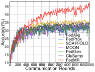
(a) $\alpha=0.1$

(b) $\alpha=0.5$

(c) $\alpha=1.0$

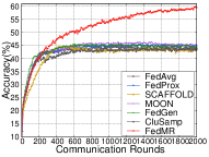
(d) IID

Figure 8: Learning curves of FL methods based on the ResNet-20 model for CIFAR-100 dataset.

Comparison of Model Convergence        Figure 8 presents the convergence trends of the seven FL methods (including FedMR) on the CIFAR-100 dataset. Note that here the training of FedMR is based on our proposed two-stage training scheme, where the first stage uses 100 FL training rounds to achieve a pre-trained model. Here, to enable fair comparison, the test accuracy of FedMR at some FL training round is calculated by an intermediate global model, which is an aggregated version of all the local models within that round. The four sub-figures show the results for different data distributions of clients. From this figure, we can find that FedMR outperforms the other six FL methods consistently in both non-IID and IID scenarios. This is mainly because FedMR can easily escape from the stuck-at-local-search due to the model recombination operation in each FL round. Moreover, due to the fine-grained training, we can observe that the learning curves in each sub-figure are much smoother than the ones of other FL methods. We also conducted the comparison for CNN- and VGG-16-based FL methods, and found similar observations from them. Please refer to Appendix C.2 for more details.

5.4 Ablation Study

Impacts of Activated Clients        Figure 9 compares the learning trends between FedMR and six baselines for a non-IID scenario ($\alpha=0.1$) with both ResNet-20 model and CIFAR-10 dataset, where the numbers of activated clients are $5$, $10$, $20$, $50$, and $100$, respectively. From Figure 9, we can observe that FedMR achieves the best inference performance for all cases. When the number of activated clients increases, the convergence fluctuations reduce significantly. Please refer to Appendix C.2 for more results on IID scenarios.

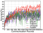
(a) $K=5$

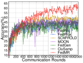
(b) $K=10$

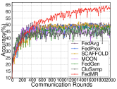
(c) $K=20$

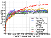
(d) $K=50$

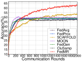
(e) $K=100$

Figure 9: Comparison of FL methods using ResNet-20 model on CIFAR-10 dataset with $\alpha=0.1$.

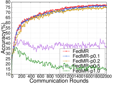
(a) ResNet-20

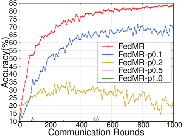
(b) VGG-16

Figure 10: Learning curves for different partitioning strategies.

Impacts of Model Layer Partitioning To show the effectiveness of our layer-wise model recombination scheme, we evaluated the FedMR performance using different model layer partitioning strategies. We use “FedMR-p$x$” to denote that the model is divided into $\lceil\frac{1}{x}\rceil$ ($x\in(0,1.0]$) segments, where the model recombination is based on segments rather than layers. Note that $x=1.0$ indicates an extreme case, where local models are randomly dispatched to clients without recombination.

Figure 10 presents the ablation study results on CIFAR-10 dataset using ResNet-20-based and VGG-16-based FedMR, where the data on clients are non-IID distributed ($\alpha=1.0$). Note that, all the cases here did not use the two-stage training scheme. From this figure, we can find that FedMR outperforms the other variants significantly. Moreover, when the granularity of partitioning goes coarser, the classification performance of FedMR becomes worse.

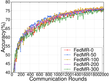
(a) ResNet-20

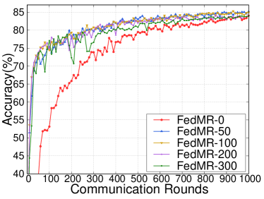
(b) VGG-16

Figure 11: Learning curves for different two-stage training settings.

Two-stage Training Scheme. To demonstrate the effectiveness of our proposed two-stage training scheme, we conducted experiments on CIFAR-10 dataset using ResNet-20-based and VGG-16-based FedMR, where the data on clients are non-IID distributed ($\alpha=1.0$). Figure 11 presents the learning trends of FedMR with five different two-stage training settings. Here, we use the notation “FedMR-$n$” to denote that the first stage involves $n$ rounds of model aggregation-based local training to obtain a pre-trained global model, while the remaining rounds conduct local training based on our proposed model recombination-based method. From Figure 11, we can observe that the two-stage training-based FedMR methods (i.e., FedMR-50 and FedMR-100) achieve the best performance from the perspectives of test accuracy and convergence rate. Note that our two-stage training scheme can achieve a more significant improvement on the case using VGG-16 model, which has a much larger size than ResNet-20 model. This is because the fine-grained FedMR without the first-stage training is not good at dealing with large-size models at the beginning of FL training, which requires much more training rounds than the coarse-grained aggregation-based methods to achieve a given preliminary classification accuracy target. By resorting to the two-stage training scheme, such a slow convergence problem can be greatly mitigated.

6 Conclusion

Due to the coarse-grained aggregation of FedAvg as well as the uniform client model initialization, when dealing with uneven data distribution among clients, existing Federated Learning (FL) methods greatly suffer from the problem of low inference performance. To address this problem, this paper presented a new FL paradigm named FedMR, which enables different layers of local models to be trained on different clients. Since FedMR supports both fine-grained model recombination and diversified local training initialization, it enables effective and efficient search for superior generalized models for all clients. Comprehensive experimental results show both the effectiveness and pervasiveness of our proposed method in terms of inference accuracy and convergence rate.

Appendix A Proof of FedMR Convergence

A.1 Notations

In our FedMR approach, the global model is aggregated from all the recombined models and all the models have the same weight. Let $t$ exhibit the $t^{th}$ SGD iteration on the local device, $v$ is the intermediate variable that represents the result of SGD update after exactly one iteration. The update of FedMR is as follows:

$$v_{t+1}^{k}=w_{t}^{k}-\eta_{t}\nabla f_{k}(w_{t}^{k},\xi_{t}^{k}),$$ (1)

$$w_{t+1}^{k}=\left\{\begin{array}[]{rl}v_{t+1}^{k},&if\quad E\nmid t+1\\ RM(v_{t+1}^{k}),&if\quad E\mid t+1\\ \end{array},\right.$$

where $w_{t}^{k}$ represents the model of the $k^{th}$ client in the $t^{th}$ iteration. $w_{t+1}$ denotes the global model of the ${(t+1)}^{th}$ iteration. $RM(v_{t+1}^{k})$ denotes the recombined model.

Since FedMR recombines all the local models in each round and the recombination only shuffles layers of models, the parameters of recombined models are all from the models before recombination, and no parameters are discarded. Therefore, when $\quad E\mid t+1$, we can obtain the following invariants:

$$\sum_{k=1}^{K}v_{t+1}^{k}=\sum_{k=1}^{K}RM(v_{t+1}^{k})=\sum_{k=1}^{K}w_{t+1}^{k},$$ (2)

$$\sum_{k=1}^{K}||v_{t+1}^{k}-x||^{2}=\sum_{k=1}^{K}||w_{t+1}^{k}-x||^{2},$$ (3)

where $w_{t}^{k}$ is the $k^{th}$ recombined model in $(t-1)^{th}$ iteration, which is as the local model to be dispatched to $k^{th}$ client in $t^{th}$ iteration, $x$ can any vector with the same size as $v_{t}^{k}$. Similar to [34], we define two variables $\overline{v}_{t}$ and $\overline{w}_{t}$:

$$\begin{split}\overline{v}_{t}=\frac{1}{K}\sum_{k=1}^{K}v_{t}^{k},\overline{w}_{t}=\frac{1}{K}\sum_{k=1}^{k}w_{t}^{k}.\end{split}$$ (4)

Inspired by [28], we make the following definition: $g^{k}_{t}=\nabla f_{k}(w_{t}^{k};\xi_{t}^{k})$.

A.2 Proof of Lemma 4.4

Proof.

Assume $v_{t}^{k}$ has $n$ layers, we have $v_{t}^{k}=L_{1}\oplus L_{2}\oplus...\oplus L_{n}$. Let $L_{i}=[p^{v_{t}^{k}}_{(i,0)},p^{v_{t}^{k}}_{(i,1)},...,p^{v_{t}^{k}}_{(i,|L_{i}|)}]$, where $p^{v_{t}^{k}}_{(i,j)}$ denotes the $j^{th}$ parameter of the layer $L_{i}$ in the model $v_{t}^{k}$. We have

$$\begin{split}\sum_{k=1}^{K}||v_{t}^{k}-x||^{2}=\sum_{k=1}^{K}\sum_{i=1}^{n}\sum_{j=1}^{|L_{i}|}||p^{v_{t}^{k}}_{(i,j)}-p^{x}_{(i,j)}||^{2}\end{split}$$ (5)

$$\begin{split}\sum_{k=1}^{K}||w_{t}^{k}-x||^{2}=\sum_{k=1}^{K}\sum_{i=1}^{n}\sum_{j=1}^{|L_{i}|}||p^{w_{t}^{k}}_{(i,j)}-p^{x}_{(i,j)}||^{2}\end{split}$$ (6)

Since model recombination only shuffles layers of models, the parameters of recombined models are all from the models before recombination, and no parameters are discarded. We have

$$\begin{split}\forall_{i\in[1,n],j\in[1,|L_{i}|]}\sum_{k=1}^{K}p^{v_{t}^{k}}_{(i,j)}=\sum_{k=1}^{K}p^{w_{t}^{k}}_{(i,j)}\end{split}$$ (7)

$$\begin{split}\forall_{k\in[1,K],i\in[1,n],j\in[1,|L_{i}|]}\exists_{q\in[1,K]}\{{p^{v_{t}^{k}}_{(i,j)}=p^{w_{t}^{q}}_{(i,j)}}\}\end{split}$$ (8)

$$\begin{split}\forall_{k\in[1,K],i\in[1,n],j\in[1,|L_{i}|]}\exists_{q\in[1,K]}\{{p^{w_{t}^{k}}_{(i,j)}=p^{v_{t}^{q}}_{(i,j)}}\}\end{split}$$ (9)

According to Equation 7-9, we have

$$\begin{split}\sum_{k=1}^{K}||v_{t}^{k}-x||^{2}&=\sum_{k=1}^{K}\sum_{i=1}^{n}\sum_{j=1}^{|L_{i}|}||p^{v_{t}^{k}}_{(i,j)}-p^{x}_{(i,j)}||^{2}\\ &=\sum_{k=1}^{K}\sum_{i=1}^{n}\sum_{j=1}^{|L_{i}|}||p^{w_{t}^{k}}_{(i,j)}-p^{x}_{(i,j)}||^{2}\\ &=\sum_{k=1}^{K}||w_{t}^{k}-x||^{2}\\ \end{split}$$ (10)

∎

A.3 Key Lemmas

To facilitate the proof of our theorem, we present the following lemmas together with their proofs.

Lemma A.1.

(Results of one step SGD). If $\eta_{t}\leq\frac{1}{4L}$, we have

$$\begin{split}\mathbb{E}||\overline{v}_{t+1}-w^{\star}||^{2}\leq\frac{1}{K}\sum_{k=1}^{K}(1-\mu\eta_{t})||v^{k}_{t}-w^{\star}||^{2}+\frac{1}{K}\sum_{k=1}^{K}||w^{k}_{t}-w^{k}_{t_{0}}||^{2}+10\eta_{t}^{2}L\Gamma\end{split}.$$

Proof.

According to Equation 2 and Equation 3, we have

$$\begin{split}||\overline{v}_{t+1}-w^{\star}||^{2}&\leq\frac{1}{K}\sum_{k=1}^{K}||v^{k}_{t+1}-w^{\star}||^{2}\\ &=\frac{1}{K}\sum_{k=1}^{K}||v^{k}_{t}-\eta_{t}g^{k}_{t}-w^{\star}||^{2}\\ &=\frac{1}{K}\sum_{k=1}^{K}(||v^{k}_{t}-w^{\star}||^{2}-2\eta_{t}\langle w^{k}_{t}-w^{\star},g^{k}_{t}\rangle+\eta_{t}^{2}||g^{k}_{t}||^{2})\end{split}$$ (11)

Let $B_{1}=-2\eta_{t}\langle w^{k}_{t}-w^{\star},g^{k}_{t}\rangle$ and $B_{2}=\eta_{t}^{2}\sum_{k=1}^{K}||g^{k}_{t}||^{2}$. According to Assumption 4.2, we have

$$B_{1}\leq-2\eta_{t}(f_{k}(w^{k}_{t})-f_{k}(w^{\star}))-\mu\eta_{t}||w^{k}_{t}-w^{\star}||^{2}$$ (12)

According to Assumption 4.1, we have

$$B_{2}\leq 2\eta_{t}^{2}L(f_{k}(w_{t}^{k})-f_{k}^{\star})$$ (13)

According to Equation 12 and 13, we have

$$||\overline{v}_{t+1}-w^{\star}||^{2}\leq\frac{1}{K}\sum_{k=1}^{K}[(1-\mu\eta_{t})||v^{k}_{t}-w^{\star}||^{2}-2\eta_{t}(f_{k}(w^{k}_{t})-f_{k}(w^{\star}))+2\eta_{t}^{2}L(f_{k}(w_{t}^{k})-f_{k}^{\star})]$$ (14)

Let $C=\frac{1}{K}\sum_{k=1}^{K}[-2\eta_{t}(f_{k}(w^{k}_{t})-f_{k}(w^{\star}))+2\eta_{t}^{2}L(f_{k}(w_{t}^{k})-f_{k}^{\star})]$. We have

$$\begin{split}C&=\frac{-2\eta_{t}}{K}\sum_{k=1}^{K}(f_{k}(w^{k}_{t})-f_{k}(w^{\star}))+\frac{2\eta_{t}^{2}L}{K}\sum_{k=1}^{K}(f_{k}(w_{t}^{k})-f_{k}^{\star})\\ &=-\frac{2\eta_{t}(1-\eta_{t}L)}{K}\sum_{k=1}^{K}(f_{k}(w^{k}_{t})-f^{\star})+\frac{2\eta_{t}^{2}L}{K}\sum_{k=1}^{K}(f^{\star}-f^{\star}_{k})\end{split}$$ (15)

Let $\Gamma=f^{\star}-\frac{1}{K}\sum_{k=1}^{K}f^{\star}_{k}$ and $\phi=2\eta_{t}(1-L\eta_{t})$. We have

$$C=-\frac{\phi}{K}\sum_{k=1}^{K}(f_{k}(w^{k}_{t})-f^{\star})+2\eta_{t}^{2}L\Gamma$$ (16)

Let $D=-\frac{1}{K}\sum_{k=1}^{K}(f_{k}(w^{k}_{t})-f^{\star})$, $E\mid t_{0}$ and $t-t_{0}\leq E$. We have

$$\begin{split}D=-\frac{1}{K}\sum_{k=1}^{K}(f_{k}(w^{k}_{t})-f_{k}(w^{k}_{t_{0}})+f_{k}(w^{k}_{t_{0}})-f^{\star})\end{split}$$ (17)

By Cauchy–Schwarz inequality, we have

$$\begin{split}D&\leq\frac{1}{2K}\sum_{k=1}^{K}(\eta_{t}||\nabla f_{k}(w^{k}_{t_{0}})||^{2}+\frac{1}{\eta_{t}}||w^{k}_{t}-w^{k}_{t_{0}}||^{2})-\frac{1}{K}\sum_{k=1}^{K}(f_{k}(w^{k}_{t_{0}})-f^{\star})\\ &\leq\frac{1}{2K}\sum_{k=1}^{K}[2\eta_{t}L(f_{k}(w^{k}_{t_{0}})-f_{k}^{\star})+\frac{1}{\eta_{t}}||w^{k}_{t}-w^{k}_{t_{0}}||^{2}]-\frac{1}{K}\sum_{k=1}^{K}(f_{k}(w^{k}_{t_{0}})-f^{\star})\end{split}$$ (18)

Note that since $\eta\leq\frac{1}{4L}$, $\eta_{t}\leq\phi\leq 2\eta_{t}$ and $\eta_{t}L\leq\frac{1}{4}$. According to Equation 18, we have

$$\begin{split}C&\leq\frac{\phi}{2K}\sum_{k=1}^{K}[2\eta_{t}L(f_{k}(w^{k}_{t_{0}})-f_{k}^{\star})+\frac{1}{\eta_{t}}||w^{k}_{t}-w^{k}_{t_{0}}||^{2}]-\frac{\phi}{K}\sum_{k=1}^{K}(f_{k}(w^{k}_{t_{0}})-f^{\star})+\eta_{t}^{2}L\Gamma\\ &=\frac{\phi}{2\eta_{t}K}\sum_{k=1}^{K}||w^{k}_{t}-w^{k}_{t_{0}}||^{2}+(\phi\eta_{t}L+2\eta_{t}^{2}L)\Gamma+\frac{\phi}{K}\sum_{k=1}^{K}(f^{\star}-f_{k}(w^{k}_{t_{0}}))\\ &\leq\frac{\phi}{2\eta_{t}K}\sum_{k=1}^{K}||w^{k}_{t}-w^{k}_{t_{0}}||^{2}+(\phi\eta_{t}L+2\eta_{t}^{2}L)\Gamma+\frac{\phi}{K}\sum_{k=1}^{K}(f^{\star}-f_{k}^{\star})\\ &\leq\frac{\phi}{2\eta_{t}K}\sum_{k=1}^{K}||w^{k}_{t}-w^{k}_{t_{0}}||^{2}+(\phi\eta_{t}L+\phi+2\eta_{t}^{2}L)\Gamma\\ &\leq\frac{1}{K}\sum_{k=1}^{K}||w^{k}_{t}-w^{k}_{t_{0}}||^{2}+(2\eta_{t}^{2}L+2\eta_{t})\Gamma\\ &\leq\frac{1}{K}\sum_{k=1}^{K}||w^{k}_{t}-w^{k}_{t_{0}}||^{2}+10\eta_{t}^{2}L\Gamma\end{split}$$ (19)

∎

Lemma A.2.

Within our configuration, the model recombination occurs every $E$ iterations. For arbitrary t, there always exists $t_{0}\leq t$ while $t_{0}$ is the nearest recombination to $t$. As a result, $t-t_{0}\leq E-1$ holds. Given the constraint on learning rate from [28], we know that $\eta_{t}\leq\eta_{t_{0}}\leq 2\eta_{t}$. It follows that

$$\begin{split}\frac{1}{K}\sum_{k=1}^{K}||w_{t}^{k}-{w}^{k}_{t_{0}}||^{2}\leq 4\eta_{t}^{2}(E-1)^{2}G^{2}.\end{split}$$

Proof.

$$\begin{split}\frac{1}{K}\sum_{k=1}^{K}||w_{t}^{k}-{w}^{k}_{t_{0}}||^{2}=&\frac{1}{K}\sum_{k=1}^{K}||\sum_{t=t_{0}}^{t_{0}+E-1}\eta_{t}\nabla f_{a_{1}}(w_{t}^{a_{1}};\xi_{t}^{a_{1}})||^{2}\\ &\leq(t-t_{0})\sum_{t=t_{0}}^{t_{0}+E-1}\eta_{t}^{2}G^{2}\\ &\leq(E-1)\sum_{t=t_{0}}^{t_{0}+E-1}\eta_{t}^{2}G^{2}\\ &\leq 4\eta_{t}^{2}(E-1)^{2}G^{2}.\end{split}$$

∎

A.4 Proof of Theorem 1

Proof.

Let $\Delta_{t}=||\overline{w}_{t}-w^{\star}||^{2}$ and $\Delta^{\sum}_{t}=\frac{1}{K}\sum_{k=1}^{K}||w_{t}^{k}-{w}^{\star}||^{2}$.

According to Lemma A.1 and Lemma A.2, we have

$$\begin{split}\Delta_{t+1}\leq\Delta^{\sum}_{t+1}\leq(1-\mu\eta_{t})\Delta^{\sum}_{t}+\eta_{t}^{2}B\end{split},$$

where

$$\begin{split}B=10L\Gamma+4(E-1)^{2}G^{2}\end{split}.$$

When the step size is diminish, let $\eta_{t}=\frac{\beta}{t+\gamma}$, where $\beta>\frac{1}{\mu}$, $\gamma>0$ such that $\eta_{t}\leq min\{\frac{1}{\mu},\frac{1}{4L}\}=\frac{1}{4L}$ and $\eta_{t}\leq 2\eta_{t+E}$.

Let $\psi=max\{\frac{\beta^{2}B}{\mu\beta-1},(\gamma+1)\Delta_{1}\}$, we firstly proof $\Delta_{t}\leq\frac{\psi}{t+\gamma}$. For $t=1$,

$$\Delta_{1}=\Delta^{\sum}_{1}=\frac{\gamma+1}{\gamma+1}\Delta_{1}\leq\frac{\psi}{\gamma+1}$$ (20)

Assume that $\Delta_{t}\leq\Delta^{\sum}_{t}\leq\frac{\psi}{\gamma+1}$,

$$\begin{split}\Delta_{t+1}&\leq\Delta^{\sum}_{t+1}\\ &\leq(1-\mu\eta_{t})\Delta^{\sum}_{t}+\eta_{t}^{2}B\\ &=(1-\frac{\mu\beta}{t+\gamma})\frac{\psi}{t+\gamma}+\frac{\beta^{2}B}{(t+\gamma)^{2}}\\ &\leq\frac{t+\gamma-1}{(t+\gamma)^{2}}\psi+[\frac{\beta^{2}B}{(t+\gamma)^{2}}-\frac{\mu\beta-1}{(t+\gamma)^{2}}\psi]\\ &\leq\frac{t+\gamma-1}{(t+\gamma)^{2}}\psi+[\frac{\beta^{2}B}{(t+\gamma)^{2}}-\frac{\mu\beta-1}{(t+\gamma)^{2}}\frac{\beta^{2}B}{\mu\beta-1}]\\ &\leq\frac{\psi}{t+1+\gamma}.\end{split}$$ (21)

According to Equation 20 and Equation 21, we have

$$\Delta_{t}\leq\frac{\psi}{t+\gamma}.$$ (22)

According to Assumption 4.1 and Equation 22, we have

$$\mathbb{E}[f(\overline{w}_{t})]-f^{\star}\leq\frac{L}{2}\Delta_{t}\leq\frac{\psi L}{2(t+\gamma)}$$ (23)

If we set $\beta=\frac{2}{\mu}$ and $\gamma=max\{\frac{10L}{\mu},E\}-1$, we have $\eta_{t}=\frac{2}{\mu(t+\gamma)}$ and $\eta_{t}\leq 2\eta_{t+E}$ for $t\geq 1$.

Then we have

$$\psi=max\{\frac{\beta^{2}B}{\mu\beta-1},(\gamma+1)\Delta_{1}\}\leq\frac{\beta^{2}B}{\mu\beta-1}+(\gamma+1)\Delta_{1}\leq\frac{4B}{\mu^{2}}+(\gamma+1)\Delta_{1}$$ (24)

According to Equation 23 and Equation 24, we have

$$\mathbb{E}[f(\overline{w}_{t})]-f^{\star}\leq\frac{L}{2(t+\gamma)}[\frac{4B}{\mu^{2}}+(\gamma+1)\Delta_{1}]=\frac{L}{2\mu(t+\gamma)}[\frac{4B}{\mu}+\frac{\mu(\gamma+1)}{2}\Delta_{1}]$$ (25)

∎

Appendix B Secure Model Recombination Mechanism

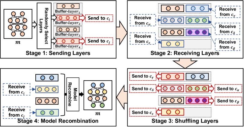
Figure 12: Workflow of secure model recombination mechanism.

To avoid the risk of privacy leakage caused by exposing gradients or models to the cloud server, we propose a secure model recombination mechanism for FedMR, which allows the random exchange of model layers among clients before model training or upload. As shown in Figure 12, within a round of the secure model recombination, the update of each model (i.e., $m$) consists of four stages:

Stage 1: Assume that the local model has $len$ layer. Each client maintains a buffer for each layer. Firstly, each client randomly selects a part of its layers and sends them to other activated clients, while the remaining layers are saved in their corresponding buffers. Note that a selected layer can only be sent to one client. For example, in Figure 12, the client $m$ sends $layer_{2}$ and $layer_{4}$ to $c_{i}$ and $c_{j}$, respectively.

Stage 2: Once receiving a layer from other client, the receiving client $m$ will add the layer to its corresponding buffer. For example, in Figure 12, the client $m$ totally receives five layers. Besides the retained two layers in stage 1, $m$ now has seven layers in total in its buffers.

Stage 3: For each layer buffer of $m$, if there contains one element received from a client $c$ in stage 2, our mechanism will randomly select one layer in the buffer and return it back to $c$. For example, in Figure 12, $m$ randomly returns a layer in Buffer-layer1 back to a client $c_{\gamma}$.

Stage 4: Once receiving the returned layers from other clients, our mechanism will recombine them with all the other layers in the buffers to form a new model. Note that the recombined model may be significantly different from the original model in Stage 1.

Note that each FL training round can perform multiple times secure model recombination. Due to the randomness, it is hard for adversaries to figure out the sources of client model layers.

B.1 Implementation

Algorithm 2 presents the implementation of our secure model recombination mechanism. The input $r_{s}$ denotes the number of repeat times and Lines 2-26 presents the process of one time of secure model recombination. Since the number of sending layers for each client is random, in our implementation, we set a low bound $n_{l}$ and an upper bound $n_{u}$. In Line 2, the client randomly generates $n$ from $[n_{l},n_{u}]$ at the beginning of each time of secure model recombination. Line 3 initializes layer buffers, where $Buf_{l}$ is a list of lists, which consists of $len(w)$ lists. $len(w)$ denotes the number of layers in $w$. Line 4 initializes the client buffer $Buf_{c}$, which is used to store the host and type of received layers. Therefore, elements of $Buf_{c}$ are two tuples $\langle c,idx_{l}\rangle$, where $c$ denotes a client and $idx_{l}$ denotes the index of a layer.

Stage 1 (Lines 5-10): In Line 5, the client randomly selects $n$ layers from its model. Lines 6-10 randomly send selected layers to activated clients. Line 7 randomly selects an activated client $c$ from $L_{a}$. Then, in Line 8, the client sends the $i^{th}$ layer in $L_{layer}$ to $c$. Line 9 removes the sent layer from layer buffers.

Stage 2 (Lines 11-14): When receiving a layer $l_{j}$ from a client $c$, Line 12 pushes the layer into the corresponding layer buffer and Line 13 pushes the client with the index of the received layer as a two-tuple $\langle c,j\rangle$ into $Buf_{c}$.

Stage 3 (Lines 15-19): Line 15 gets an element $\langle c,j\rangle$ from $Buf_{c}$. Line 16 randomly selects a layer $l$ with index $j$ from layer buffer $Buf_{l}[j]$. Line 17 sends the selected layer $l$ to $c$. Line 18 removes $l$ from $Buf_{l}[j]$.

Stage 4 (Lines 20-26): Lines 20-22 receive layers from activated clients. Note that such clients are the same as the clients selected in Line 7. Line 21 pushes the received layer into layer buffers. Lines 23-26 recombine layers in layer buffers to generate a new model. Note that, since the number and type of sent layers are equal to that of received layers, after Line 22, each list in $Buf_{l}$ has only one layer. Line 24 pulls the $i^{th}$ layer $l$ from $Buf_{l}$ and Line 25 replaces the $i^{th}$ layer in $w$ with $l$.

To further prevent privacy leakage, the cloud server will broadcast a public key before the secure recombination. By using the public key to encrypt the model parameters of each layer, the other clients cannot directly obtain their received parameters.

Algorithm 2 Secure Model Recombination

Input: i) $r_{s}$, # of repeat times; ii) $idx$, index of the client; iii) $w$, parameters of the model in client $idx$; iv) $L_{a}$, the list of activated clients; v) $n_{l}$, the low bound of # of sending layer; vi) $n_{u}$, the upper bound of # of sending layer.
Output: $w$, the parameters of the recombined model.
SecMR($rnd$,$S_{dev}$,$K$)

1:  for $r$ = 1, …, $r_{s}$ do

2:     $n\leftarrow$ Random($n_{l},n_{u}$);

3:     $Buf_{l}\leftarrow[[w[1]],[w[2]],...,[w[len(w)]]]$;

4:     $Buf_{c}\leftarrow[]$; /* Stage 1 start */

5:     $L_{layer}\leftarrow$ Random select $n$ layers from $w$;

6:     for $i$ = 1, …, $n$ do

7:        $c\leftarrow$ Random select a client in $L_{a}$;

8:        Send layer $L_{layer}[i]$ to client $c$;

9:        Remove $L_{layer}[i]$ from $Buf_{l}[i]$;

10:     end for /* Stage 2 start */

11:     while Receive layer $l_{j}$ from a client $c$ do

12:        $Buf_{l}[j].append(l_{j})$;

13:        $Buf_{c}.append(<c,j>)$;

14:     end while/* Stage 3 start*/

15:     for $<c,j>$ in $Buf_{c}$ do

16:        $l\leftarrow$ Random select a layer in $Buf_{l}[j]$;

17:        Send layer $l$ to client $c$;

18:        Remove $l$ from $Buf_{l}[j]$;

19:     end for /* Stage 4 start*/

20:     while Receive layer $l_{j}$ from a client $c$ do

21:        $Buf_{l}[j].append(l_{j})$;

22:     end while

23:     for $i=1,2,...,len(w)$ do

24:        $l\leftarrow Buf_{l}[i][0]$;

25:        $w[i]\leftarrow l$;

26:     end for

27:  end for 

B.2 Discussions

B.2.1 Privacy Preserving

Since clients received layers are encrypted by the public key from the cloud server, they cannot directly obtain the model parameters of other clients. Note that, only in Stage 2 of the first time of secure model recombination clients can distinguish the source of received layers. Since layers sent in Stage 3 are randomly selected, clients cannot distinguish the received layers in Stage 4 from senders or other clients. Therefore, even if there are multiple malicious clients colluding with the cloud, it can only distinguish the source of the $n_{u}$ layer at most for each client. Since models received by the cloud server are recombined, the cloud server cannot restore the original model of each client. Based on the above analysis, we suggest that each client set a small $n_{u}$ at the first time of secure recombination and conduct multiple times of secure recombination before uploading its model.

B.2.2 Communication Overhead

At each time of secure model recombination, each client sends $n\in[n_{l},n_{u}]$ layers to other clients in Stage 1 and receives $n$ layers from other clients in Stage 4. Note that layers received in Stage 2 are from layers sent in Stage 1 and layers received in Stage 4 are from layers sent in Stage 3. Therefore the communication overhead of a time of secure model recombination can be presented as

$$\begin{split}\sum_{k=1}^{K}2\sum_{j=1}^{n_{k}}size(l_{k,j}).\end{split}$$ (26)

Since $n_{k}\in[n_{l},n_{u}]$ where $n_{l}>0$ and $n_{u}\leq len(w)$, and each layer can only be sent to one client, we have

$$\begin{split}\mathbb{E}\sum_{k=1}^{K}2\sum_{j=1}^{n_{k}}size(l_{k,j})=\frac{(n_{u}+n_{l})K}{len(w)}\times size(w)\leq\frac{2n_{u}K}{len(w)}\times size(w)\leq 2K\times size(w).\end{split}$$ (27)

From Equation 27, we can find as the increase of $n_{l}+n_{u}$, the expectation of communication overhead of secure recombination increases linearly.

Appendix C Experimental Results and Discussions

C.1 Extended Performance Comparison

Comparison of Communication Overhead: Let $K$ be the number of activated clients in each FL training round. Since the cloud server needs to send $K$ recombined models to $K$ clients and receive $K$ trained local models from $K$ clients in an FL round, the communication overhead of FedMR is $2K$ models in each round, which is the same as FedAvg, FedProx, and CluSamp. Since the cloud server needs to dispatch an extra global control variable to each client and clients also need to update and upload these global control variables to the cloud server, the communication overhead of SCAFFOLD is $2K$ models plus $2K$ global control variables in each FL training round. Unlike the other FL methods, the cloud server of FedGen needs to dispatch an additional built-in generator to the selected clients, the communication overhead of FedGen in each FL training round is $2K$ models plus $K$ generators. Base on the above analysis, we can find that FedMR does not cause any extra communication overhead. Therefore, FedMR requires the least communication overhead among all the investigated FL methods in each FL training round. Note that, as shown in Figure 8, although FedMR requires more rounds to achieve the highest test accuracy, to achieve the highest accuracy of other FL methods, FedMR generally requires less FL rounds. In other words, to achieve the same test accuracy, FedMR requires much fewer overall communication overhead.

Comparison of Computing Overhead: Let $l_{n}$ be the number of layers of a model, and $P$ be the number of parameters of a model. For FedMR, in each FL training round, the cloud server needs to calculate $l_{n}\times K$ random numbers for shuffling, and each recombination needs to move $K\times P$ model parameters. Since $l_{n}\ll P$, the overall complexity of one FedMR round is $O(K\times P)$ for the cloud server. Note that FedMR does not cause additional computing overhead to the client. For FedAvg, the overall complexity of each FL training round is also $O(K\times P)$, since it needs to aggregate all the local models. Therefore FedMR has a similar computing overhead as FedAvg. Since CluSamp requires cluster clients, its complexity in the cloud server is $O(K^{2}\times P)$. Since all the other baselines conduct FedAvg-based aggregation, the computation overhead of the cloud server for them is similar to FedAvg. However, since FedProx, SCAFFOLD, MOON, and FedGen require clients to conduct additional computations, their overall computing overhead is more than those of FedAvg and FedMR.

C.2 Experimental Results for Accuracy Comparison

In this section, we present all the experimental results. Figure 13-15 compare the learning curves of FedMR with all the six baselines based on the CNN, ResNet-20, and VGG-16, respectively. Figure 16-17 compare the learning curves of FedMR with all the six baselines with different numbers of activated clients based on the ResNet-20 model for CIFAR-10 dataset with IID scenario and non-IID scenario with $\alpha=0.1$, respectively.

C.3 Discussions

C.3.1 Privacy Preserving

Similar to traditional FedAvg-based FL methods, FedMR does not require clients to send their data to the cloud server, thus the data privacy can be mostly guaranteed by the secure clients themselves. Someone may argue that dispatching the recombined models to adversarial clients may expose the privacy of some clients by attacking their specific layers. However, since our model recombination operation breaks the dependencies between model layers and conducts the shuffling of layers among models, in practice it is hard for adversaries to restore the confidential data from a fragmentary recombined model without knowing the sources of layers. Our secure recombination mechanism ensures that the cloud server only received recombined models from clients, which means the cloud server cannot restore the model of each client.

C.3.2 Limitations

As a novel FL paradigm, FedMR shows much better inference performance than most SOTA FL methods. Although this paper proposed an efficient two-stage training scheme to accelerate the overall FL training processes, there still exists numerous chances (e.g., client selection strategies, dynamic combination of model aggregation and model recombination operations) to enable further optimization on the current version of FedMR. Meanwhile, the current version of FedMR does not take personalization into account, which is also a very important topic that is worthy of studying in the future.

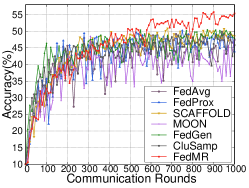
(a) CIFAR-10 with $\alpha=0.1$

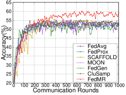
(b) CIFAR-10 with $\alpha=0.5$

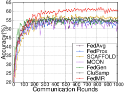
(c) CIFAR-10 with $\alpha=1.0$

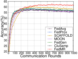
(d) CIFAR-10 with IID

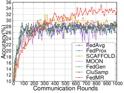
(e) CIFAR-100 with $\alpha=0.1$

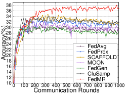
(f) CIFAR-100 with $\alpha=0.5$

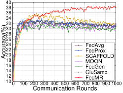
(g) CIFAR-100 with $\alpha=1.0$

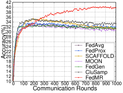
(h) CIFAR-100 with IID

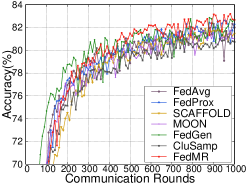
(i) FEMNIST

Figure 13: Learning curves of different FL methods based on the CNN model.

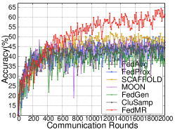
(a) CIFAR-10 with $\alpha=0.1$

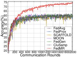
(b) CIFAR-10 with $\alpha=0.5$

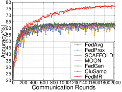
(c) CIFAR-10 with $\alpha=1.0$

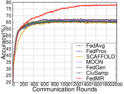
(d) CIFAR-10 with IID

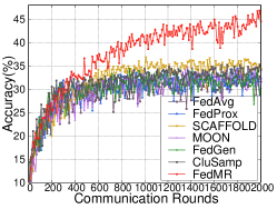
(e) CIFAR-100 with $\alpha=0.1$

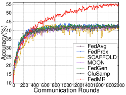
(f) CIFAR-100 with $\alpha=0.5$

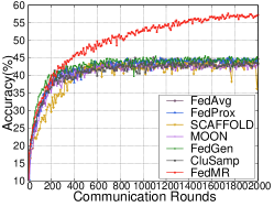
(g) CIFAR-100 with $\alpha=1.0$

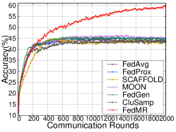
(h) CIFAR-100 with IID

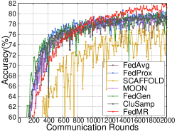
(i) FEMNIST

Figure 14: Learning curves of different FL methods based on the ResNet-20 model.

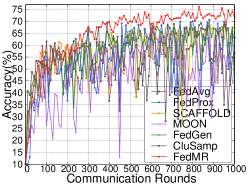
(a) CIFAR-10 with $\alpha=0.1$

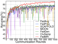
(b) CIFAR-10 with $\alpha=0.5$

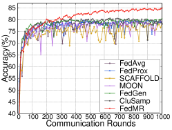
(c) CIFAR-10 with $\alpha=1.0$

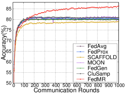
(d) CIFAR-10 with IID

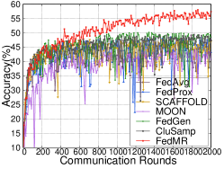
(e) CIFAR-100 with $\alpha=0.1$

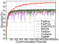
(f) CIFAR-100 with $\alpha=0.5$

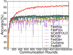
(g) CIFAR-100 with $\alpha=1.0$

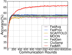
(h) CIFAR-100 with IID

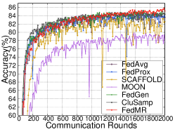
(i) FEMNIST

Figure 15: Learning curves of different FL methods based on the VGG-16 model.

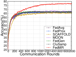
(a) $K=5$

(b) $K=10$

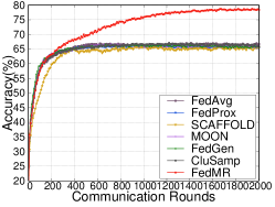
(c) $K=20$

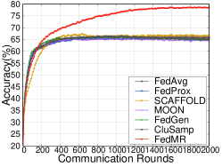
(d)

$$K=50$$

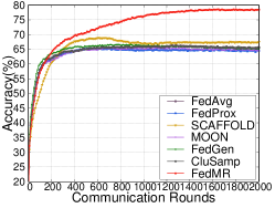
(e) $K=100$

Figure 16: Learning curves of different FL methods based on the ResNet-20 model for CIFAR-10 dataset with IID scenario.

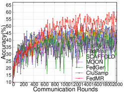
(a) $K=5$

(b) $K=10$

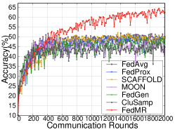
(c) $K=20$

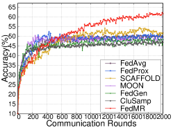
(d) $K=50$

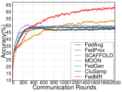
(e) $K=100$

Figure 17: Learning curves of different FL methods based on the ResNet-20 model for CIFAR-10 dataset with $\alpha=0.1$.

References

- McMahan et al. [2017] Brendan McMahan, Eider Moore, Daniel Ramage, Seth Hampson, and Blaise Aguera y Arcas. Communication-efficient learning of deep networks from decentralized data. In Proceedings of Artificial intelligence and statistics, pages 1273–1282, 2017.
- Zhang et al. [2020] Xinqian Zhang, Ming Hu, Jun Xia, Tongquan Wei, Mingsong Chen, and Shiyan Hu. Efficient federated learning for cloud-based aiot applications. IEEE Transactions on Computer-Aided Design of Integrated Circuits and Systems, 40(11):2211–2223, 2020.
- Elayan et al. [2021] Haya Elayan, Moayad Aloqaily, and Mohsen Guizani. Sustainability of healthcare data analysis iot-based systems using deep federated learning. IEEE Internet of Things Journal, 9(10):7338–7346, 2021.
- Liu et al. [2021] Quande Liu, Cheng Chen, Jing Qin, Qi Dou, and Pheng-Ann Heng. Feddg: Federated domain generalization on medical image segmentation via episodic learning in continuous frequency space. In Proceedings of the IEEE/CVF Conference on Computer Vision and Pattern Recognition, pages 1013–1023, 2021.
- Yang et al. [2021] Qian Yang, Jianyi Zhang, Weituo Hao, Gregory P Spell, and Lawrence Carin. Flop: Federated learning on medical datasets using partial networks. In Proceedings of the ACM SIGKDD Conference on Knowledge Discovery & Data Mining, pages 3845–3853, 2021.
- Leroy et al. [2019] David Leroy, Alice Coucke, Thibaut Lavril, Thibault Gisselbrecht, and Joseph Dureau. Federated learning for keyword spotting. In Proceedings of IEEE International Conference on Acoustics, Speech and Signal Processing (ICASSP), pages 6341–6345, 2019.
- Agarwal et al. [2021] Naman Agarwal, Peter Kairouz, and Ziyu Liu. The skellam mechanism for differentially private federated learning. Advances in Neural Information Processing Systems, 34:5052–5064, 2021.
- Zhao et al. [2022] Bo Zhao, Peng Sun, Tao Wang, and Keyu Jiang. Fedinv: Byzantine-robust federated learning by inversing local model updates. In Proceedings of the AAAI Conference on Artificial Intelligence, volume 36, pages 9171–9179, 2022.
- Zhou et al. [2022] Chendi Zhou, Ji Liu, Juncheng Jia, Jingbo Zhou, Yang Zhou, Huaiyu Dai, and Dejing Dou. Efficient device scheduling with multi-job federated learning. In Proceedings of the AAAI Conference on Artificial Intelligence, volume 36, pages 9971–9979, 2022.
- Kairouz et al. [2021] Peter Kairouz, H Brendan McMahan, Brendan Avent, Aurélien Bellet, Mehdi Bennis, Arjun Nitin Bhagoji, Kallista Bonawitz, Zachary Charles, Graham Cormode, Rachel Cummings, et al. Advances and open problems in federated learning. Foundations and Trends® in Machine Learning, 14(1–2):1–210, 2021.
- Wang et al. [2020] Hao Wang, Zakhary Kaplan, Di Niu, and Baochun Li. Optimizing federated learning on non-iid data with reinforcement learning. In Proceedings of IEEE Conference on Computer Communications, pages 1698–1707, 2020.
- Acar et al. [2020] Durmus Alp Emre Acar, Yue Zhao, Ramon Matas, Matthew Mattina, Paul Whatmough, and Venkatesh Saligrama. Federated learning based on dynamic regularization. In Proceedings of International Conference on Learning Representations, 2020.
- Xie et al. [2020] Ming Xie, Guodong Long, Tao Shen, Tianyi Zhou, Xianzhi Wang, Jing Jiang, and Chengqi Zhang. Multi-center federated learning. arXiv preprint arXiv:2005.01026, 2020.
- Karimireddy et al. [2020] Sai Praneeth Karimireddy, Satyen Kale, Mehryar Mohri, Sashank Reddi, Sebastian Stich, and Ananda Theertha Suresh. Scaffold: Stochastic controlled averaging for federated learning. In Proceedings of International Conference on Machine Learning, pages 5132–5143, 2020.
- Huang et al. [2021] Yutao Huang, Lingyang Chu, Zirui Zhou, Lanjun Wang, Jiangchuan Liu, Jian Pei, and Yong Zhang. Personalized cross-silo federated learning on non-iid data. In Proceedings of the AAAI Conference on Artificial Intelligence (AAAI), 2021.
- Li et al. [2020a] Tian Li, Anit Kumar Sahu, Manzil Zaheer, Maziar Sanjabi, Ameet Talwalkar, and Virginia Smith. Federated optimization in heterogeneous networks. Proceedings of Machine Learning and Systems, 2:429–450, 2020a.
- Lin et al. [2020] Tao Lin, Lingjing Kong, Sebastian U Stich, and Martin Jaggi. Ensemble distillation for robust model fusion in federated learning. Advances in Neural Information Processing Systems, 33:2351–2363, 2020.
- Zhu et al. [2021] Zhuangdi Zhu, Junyuan Hong, and Jiayu Zhou. Data-free knowledge distillation for heterogeneous federated learning. In International Conference on Machine Learning, pages 12878–12889, 2021.
- Hochreiter and Schmidhuber [1994] Sepp Hochreiter and Jürgen Schmidhuber. Simplifying neural nets by discovering flat minima. Advances in neural information processing systems, 7, 1994.
- Hochreiter and Schmidhuber [1997] Sepp Hochreiter and Jürgen Schmidhuber. Flat minima. Neural computation, 9(1):1–42, 1997.
- Wu et al. [2017] Lei Wu, Zhanxing Zhu, et al. Towards understanding generalization of deep learning: Perspective of loss landscapes. arXiv preprint arXiv:1706.10239, 2017.
- Kwon et al. [2021] Jungmin Kwon, Jeongseop Kim, Hyunseo Park, and In Kwon Choi. Asam: Adaptive sharpness-aware minimization for scale-invariant learning of deep neural networks. In International Conference on Machine Learning, pages 5905–5914. PMLR, 2021.
- Chen et al. [2020] Cheng Chen, Ziyi Chen, Yi Zhou, and Bhavya Kailkhura. Fedcluster: Boosting the convergence of federated learning via cluster-cycling. In Proceedings of IEEE International Conference on Big Data (Big Data), pages 5017–5026, 2020.
- Fraboni et al. [2021] Yann Fraboni, Richard Vidal, Laetitia Kameni, and Marco Lorenzi. Clustered sampling: Low-variance and improved representativity for clients selection in federated learning. In Proceedings of International Conference on Machine Learning, pages 3407–3416, 2021.
- Hardt et al. [2016] Moritz Hardt, Ben Recht, and Yoram Singer. Train faster, generalize better: Stability of stochastic gradient descent. In International conference on machine learning, pages 1225–1234. PMLR, 2016.
- Wu et al. [2020] Dongxian Wu, Shu-Tao Xia, and Yisen Wang. Adversarial weight perturbation helps robust generalization. Advances in Neural Information Processing Systems, 33:2958–2969, 2020.
- Bonawitz et al. [2017] Keith Bonawitz, Vladimir Ivanov, Ben Kreuter, Antonio Marcedone, H Brendan McMahan, Sarvar Patel, Daniel Ramage, Aaron Segal, and Karn Seth. Practical secure aggregation for privacy-preserving machine learning. In proceedings of the 2017 ACM SIGSAC Conference on Computer and Communications Security, pages 1175–1191, 2017.
- Li et al. [2020b] Xiang Li, Kaixuan Huang, Wenhao Yang, Shusen Wang, and Zhihua Zhang. On the convergence of fedavg on non-iid data. In Proc. of International Conference on Learning Representations, 2020b.
- Li et al. [2021] Qinbin Li, Bingsheng He, and Dawn Song. Model-contrastive federated learning. In Proceedings of the IEEE/CVF Conference on Computer Vision and Pattern Recognition, pages 10713–10722, 2021.
- Krizhevsky [2009] Alex Krizhevsky. Learning multiple layers of features from tiny images. Master’s thesis, University of Tront, 2009.
- Caldas et al. [2018] Sebastian Caldas, Sai Meher Karthik Duddu, Peter Wu, Tian Li, Jakub Konečnỳ, H Brendan McMahan, Virginia Smith, and Ameet Talwalkar. Leaf: A benchmark for federated settings. arXiv preprint arXiv:1812.01097, 2018.
- Hsu et al. [2019] Tzu-Ming Harry Hsu, Hang Qi, and Matthew Brown. Measuring the effects of non-identical data distribution for federated visual classification. arXiv preprint arXiv:1909.06335, 2019.
- TorchvisionModel [2019] TorchvisionModel. Models and pre-trained weight. https://pytorch.org/vision/stable/models.html, 2019.
- Stich [2019] Sebastian Urban Stich. Local sgd converges fast and communicates little. In Proceedings of International Conference on Learning Representations, 2019.