Convex Equipartitions inspired by the little cubes operad
Pavle V. M. Blagojević
Inst. Math., FU Berlin, Arnimallee 2, 14195 Berlin, Germany Mat. Institut SANU, Knez Mihailova 36, 11001 Beograd, Serbia
blagojevic@math.fu-berlin.de and Nikola Sadovek
Inst. Math., FU Berlin, Arnimallee 2, 14195 Berlin, Germany
nikolasdvk@gmail.com
Abstract.
A decade ago two groups of authors, Karasev, Hubard & Aronov and Blagojević & Ziegler, have shown that the regular convex partitions of a Euclidean space into parts yield a solution to the generalised Nandakumar & Ramana-Rao conjecture when is a prime power.
This was obtained by parametrising the space of regular equipartitions of a given convex body with the classical configuration space.
Now, we repeat the process of regular convex equipartitions many times, first partitioning the Euclidean space into parts, then each part into parts, and so on.
In this way we obtain iterated convex equipartions of a given convex body into parts.
Such iterated partitions are parametrised by the (wreath) product of classical configuration spaces.
We develop a new configuration space – test map scheme for solving the generalised Nandakumar & Ramana-Rao conjecture using the Hausdorff metric on the space of iterated convex equipartions.
The new scheme yields a solution to the conjecture if and only if all the ’s are powers of the same prime.
In particular, for the failure of the scheme outside prime power case we give three different proofs.
The research by Pavle V. M. Blagojević leading to these results has
received funding from the Serbian Ministry of Science, Technological development and Innovations.
1. Introduction and statement of the main result
The following intriguing question was asked by Nandakumar & Ramana-Rao in a Nandakumar’s blog post [20] from 2006.
Conjecture 1.1(Nandakumar & Ramana-Rao).
Every convex polygon in the plane can be partitioned into any prescribed number of convex pieces that have equal area and equal perimeter.
Nandakumar & Ramana-Rao [21] gave an answer in case using the intermediate value theorem and proposed a proof for the case .
Bárány, Blagojević & Szűcs [2, Thm. 1.1] gave the positive answer for the case by setting an appropriate configuration space – test map (CS–TM) scheme which allowed efficient used of Fadell–Husseini ideal valued index theory.
Soberón [25, Thm. 1] solved a similar question, namely the Bárány’s conjecture of equally partitioning measures in into pieces, using Dold’s theorem [10].
Naturally, a higher dimensional extension of Conjecture 1.1 was soon after formulated in [17, Thm. 1.3], [7, Thm. 1.3].
Let be a -dimensional convex body in , let be an absolutely continuous probability measure on , let be any natural number, and let be any continuous functions on the metric space of -dimensional convex bodies in .
Then there exists a partition of into convex pieces such that equalities
and
hold for every .
In the previous statement, absolute continuity of probability measure in is meant with respect to the Lebesgue measure on , and the set of -dimensional convex bodies in is endowed with the Hausdorff metric.
Karasev, Hubard & Aronov [17] proposed a solution for the generalised Nandakumar & Ramana-Rao problem using a CS–TM scheme based on the generalised Voronoi diagrams.
The scheme was used to show that Conjecture 1.2 follows from the non-existence of an -equivariant map
(1)
where the symmetric group acts on and by permuting the points and coordinates, respectively.
Using a homological analogue of obstruction theory, they showed [17, Thm. 1.10] non-existence of the map (1) when is a prime power, and so gave the positive answer to the conjecture in this case.
Blagojević & Ziegler [7, Thm. 1.2] showed the non-existence of a map (1) if and only if is a prime power using equivariant obstruction theory.
In order to apply the method, they developed a Salvetti-type CW-model of the configuration space , which is moreover its equivariant deformation retract.
Resistance of Conjecture 1.2 to the existing topological methods is manifested in the fact that the map (1) exists whenever is not a prime power.
Blagojević, Lück & Ziegler [5, Thm. 8.3] showed the non-existence of a map (1) for a prime using an analogue of Cohen’s vanishing theorem [9, Thm. 8.2].
In this paper we develop a cohomological method for identifying new classes of solutions to the generalised Nandakumar & Ramana-Rao conjecture.
The method stems from a geometric idea of iterated generalised Voronoi diagrams.
Namely, let be a multiplicative decomposition of the total number of parts in which we want to partition the convex body.
In the first iteration the convex body is partitioned into convex pieces of equal area, and inductively, for each , in the th iteration one further divides each of the pieces into convex pieces of equal area.
We call such partitions iterated of level and type .
Our method is developed in three steps.
We begin by fixing a -dimensional convex body in
In the first step, presented in Section 2, we define a space , called the wreath product of configuration spaces, which is used to parametrise iterated partitions of level and type of .
Namely, we produce a map
(2)
where the codomain is the (metric) space of equal mass partitions of into pieces.
Moreover, our setting has an appropriate symmetry of the iterated semi-direct product of the symmetric groups, and the map (2) is equivariant with respect to it.
Now, by setting an appropriate CS–TM scheme and using the parametrisation map (2), we show that the existence of an iterated solution of level and type to the general Nandakumar & Ramana-Rao problem follows from non-existence of an -equivariant map of the form
Here denotes the relevant -representation, and is the unit sphere in it.
In the second step, which is “outsourced” to Section 6, we prove the result on continuity of partitions.
Namely, the CS–TM scheme from [17] and [7] used the fact that for a -dimensional convex body there exists a continuous -equivariant map
where denotes the convex partition of into parts of equal measure obtained from the generalised Voronoi diagram with sites encoded by .
The existence of such a map follows from the theory of optimal transport.
We generalise this fact and prove that the map
is continuous, where denotes the space of all -dimensional convex bodies in endowed with the Hausdorff metric.
Continuity of this map, stated in Theorem 6.6, is a crucial result which justifies the continuity of the parametrisation map (2), and therefore verifies the validity of the CS–TM scheme from Section 2.3.
In the final and third step, contained in Section 3, we prove the main topological result of the paper using equivariant obstruction theory.
Theorem 1.3.
Let , , and be integers. Then, an -equivariant map of the form
(3)
does not exist if and only if are powers of the same prime number.
Therefore, this result gives a complete answer to the question of effectiveness of the introduced CS–TM scheme in the following sense:
–
If all the numbers are powers of the same prime number, then an -equivariant map of the form (3) does not exist. Consequently, the CS–TM scheme guaranties existence of an iterated solution of Conjecture 1.2.
–
If are not all powers of the same prime number, then there exists an -equivariant map of the form (3), hence the CS–TM scheme is not able to give any insights into the existence of a solution to Conjecture 1.2.
In addition, using alternative arguments, we give two more proofs of the existence of the equivariant map in Theorem 1.3.
More precisely, in Section 4 we prove the existence of an equivariant map (3) using the structural map of the little cubes operad, and in Section 5 by appropriately adapting the trick of Özaydin in [22].
A direct consequence of Theorem 1.3 is a new positive solution of the generalised Nandakumar & Ramana-Rao conjecture.
Corollary 1.4(Iterated solution to generalised Nandakumar & Ramana-Rao).
Let be a -dimensional convex body in , let be an absolutely continuous probability measure on , let be integers, and let be any continuous functions on the metric space of -dimensional convex bodies in .
If are all powers of the same prime number, then there exists an iterated partition of of level and type into convex pieces such that equalities
and
hold for every .
Moreover, the proof method, as noted by Karasev [16, Thm. 1.6], implies also the following result,
Corollary 1.5.
Let be a -dimensional convex body in , let be an absolutely continuous probability measure on , let be integers, and let be any additive, continuous functions on the metric space of -dimensional convex bodies in . Then there exists an iterated partition of of level and type into convex pieces such that equalities
and
hold for every .
The idea of iterated partitions seems to have appeared first in context of the Gromov’s waist of the sphere theorem [13], [19].
There, Gromov [13, Thm. 4.4.A] considered partitions of the sphere into pieces, which were parametrised by the wreath products of spheres.
In order to obtain a slightly different waist of the sphere result, Palić [23, Thm. 5.2.5] considered partitions of the sphere into pieces indexed by the th wreath product of the configuration spaces on points.
Iterated partitions of Euclidean spaces appeared in the work of Blagojević & Soberón [6, Sec. 2], where they were parametrised by the th join of the configuration space.
For the purposes of this paper we use a more general version of the wreath product of configuration spaces, in the sense that the number of points of the configuration space in different levels do not need to coincide.
2. Spaces of Equal Mass Partitions
Let us denote by the space of all full dimensional convex bodies in the Euclidean space endowed with the Hausdorff metric and let be a convex body.
As in the statement of Conjecture 1.2, let be a probability measure on which is absolutely continuous with respect to the Lebesgue measure.
For an integer and a convex body , let us say that form a convex partition of into pieces if
–
, and
–
for each .
Note that, implicitly, , for all , because we require that .
Definition 2.1.
Let be an integer, let be a convex body, and let be a probability measure on which is absolutely continuous with respect to the Lebesgue measure. We define to be the space of all convex partitions of into pieces such that
endowed with the product Hausdorff metric induced from .
In the case of the plane, that is , the perimeter function induces an -equivariant map
which maps a partition to the vector obtained from by subtracting the average sum of all coordinates from each individual coordinate.
Thus, an equal area partition of gives a solution to the Nandakumar & Ramana-Rao conjecture if and only if it is mapped to the origin by the above map.
Analogously, in the general case , there exists a map
(4)
induced by the functions from the statement of Conjecture 1.2, which hits the origin in if and only if there is a solution to the generalised Nandakumar & Ramana-Rao conjecture.
See [17, Sec. 2] and [7, Sec. 2] for more details.
So far, not enough is known about the topology of the space to answer directly the question whether any map of the form (4) hits the origin.
However, such a question has been answered by restricting attention to a subspace of the, so called, regular partitions of , these are the ones which arise from piecewise-linear convex functions.
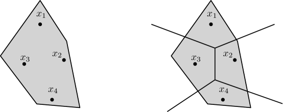
Namely, using the the theory of optimal transport (see [17, Sec. 2] and [7, Sec. 2] for more details), one can parametrise regular convex partitions of into pieces of equal area by the classical configuration space of pairwise distinct points in the plane.
For an illustration see Figure 1.
More precisely, there exists an -equivariant map
(5)
One can think of the parametrisation (5) as a prescribed way to assign to any pairwise distinct points in the plane, called the sites, a partition of into convex pieces of equal area.
In particular, if the image of the composition
(6)
of maps (5) and (4) contains the origin, there exists a regular solution to Conjecture 1.1.
Figure 1. A point induces a regular partition of the convex body .
In [17, Thm. 1.10] it was shown that whenever is a power of prime, every -equivariant map of the form
hits the origin, thus showing the existence of a solution to the (generalised) Nandakumar & Ramana-Rao conjecture in this case which is regular. Moreover, in [7, Thm. 1.2] it was shown that outside of the prime power case, there always exists an -equivariant map .
This last result used equivariant obstruction theory, and it showed the limits of the above configuration space – test map scheme proposed by the map (6).
Known topological methods are able to give solutions to the Nandakumar & Ramana-Rao conjecture in the form of regular partitions.
Since the space of convex equipartitions of is larger than the set of regular partitions of , a natural question arises: Are there solutions to the Nandakumar & Ramana-Rao conjecture which are not regular?
In this section we develop a method to parametrise iterated partitions of a given full-dimensional convex body in into parts.
Namely, we parametrise partitions with iteration by a wreath product of configuration spaces , where and .
The rest of the section is organised as follows.
In Section 2.1 we give an example of the parametrisation in the case when and .
Then, in Section 2.2, we describe partitions of level and type .
Parametrisation of such partitions by the space is presented in Section 2.3, where the configuration space – test map scheme is constructed.
2.1. Iterated partitions: first example
We establish a new configuration space – test map scheme with the intention of identifying a wider class of solutions to Conjecture 1.1.
To this end, we parametrise a class of possibly non-regular equal area partitions of into convex pieces.
In this section, we give an example of such a parametrisation for iterated partition of level two.
Let and be natural numbers such that .
Consider a parametrisation of equal are partitions of into convex pieces
(7)
obtained as the composition of the following two maps:
–
The first map
is the the product of the identity on and the parametrisation (5).
–
The second map
on each slice of the domain equals to the product of maps
for , followed by the inclusion .
In Section 6 we discuss in more details the continuity of this map.
The map (7) gives a parametrisation of equal area partition of into convex pieces which arise in two iterations.
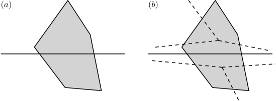
Namely, in the first iteration we divide into convex pieces by a point in according to the rule (5), and in the second iteration we again use the rule (5) to divide each of the pieces by points in .
This is an example of an iterated partition of level two and type (a,b).
For an illustration see Figure 2.
Figure 2. Partition of convex body of: level and type , level and type .
In Section 2.1 we present a more general approach and define iterated partition of level and type , for any multiplicative decomposition with .
The idea is that in the first iteration one divides into convex pieces of equal area using a point in according to the rule (5).
Continuing inductively, for each , in the th iteration one further divides each of the pieces into convex pieces of equal area by as many points in , again according to the rule (5).
Let us consider the level two example once again and discuss symmetries of the parameter space.
In this context, the natural group acting on the domain of the map (7) is the semi-direct product , where acts on the product by permuting the factors.
More precisely, the action is given by
(8)
for and , where the symmetric group acts on the configuration space by permuting the coordinates.
This action induces an action on the codomain in such a way that the parametrisation map (7) becomes -equivariant.
Indeed, an element acts on a partition
by
Thus, the expected full -symmetry of the partition is broken.
As above, the existence of a solution of the Nandakumar & Ramana-Rao conjecture parametrised by (7) will be a consequence of the fact that the composition of (7) with a perimeter-induced map into an -representation hits the origin.
Let us define such a map
(9)
which sends a partition
to a vector which:
–
for each , on the coordinates of the th copy of , has the vector
–
on the coordinates of has the vector
In analogy to (8), the actions of and on and , respectively, induce an action of the semi-direct product on the vector space , making the map (9) equivariant with respect to it.
Consequently, the -equivariant composition
of (7) and (9) hits the origin, now in , if and only if there exists an iterated solution of level two and type . In Theorem 1.3 we prove that any -equivariant map of the form
hits the origin if and only if and are powers of the same prime number. Thus, the configuration space – test map scheme is able to give a positive iterated solution of level two and type to the Nandakumar & Ramana-Rao conjecture only in the case when and are powers of the same prime.
2.2. Partition types
In this section, for integers and , we define iterated partitions of a given convex body which are of level and type .
Furthermore we identify natural groups of symmetries on such partition spaces.
For each convex body and each integer , there exists an -equivariant map
(10)
parametrising regular equal mass partitions of into convex pieces. Here we denote by the metric space of all equal mass partitions of into convex pieces. See [17, Sec. 2] or [7, Sec. 2] for more details about this map.
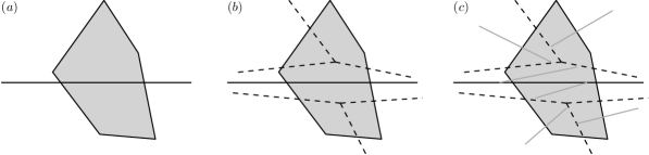
As in Section 2.1, map (10) can be thought of as a prescribed way to divide into convex parts of equal mass using pairwise distinct points in . One can now repeat the process for each of the parts individually, and divide them regularly into parts, obtaining a partition of into parts, which is not necessarily regular.
Continuing this process, each of the parts can be divided further, etc.
In this sense, regular partitions (10) can be thought of as partitions arising from a single iteration, and in the following definition we introduce a notion of a partition coming from arbitrarily many iterations.
An illustration of the iteration process see Figure 3.
Definition 2.2.
Let be a convex body.
–
(Iterated partition of level one) Let be an integer. Any partition of in the image of the map (10) is said to be iterated of level and type .
–
(Iterated partition of level ) Suppose and are integers. Let
be a partition of of level and type , and let , for , be any partition of of level and type . Then the partition
of into convex parts of equal mass is said to be iterated of level and type .
An iterated partition of level and type arises in inductive steps. For every iteration , each of the elements of the partition in the th step contains exactly elements in the partition from the st step. Therefore, the collection of all such intermediate parts forms a ranked poset with respect to inclusion. More precisely:
–
The maximum of the poset is the full convex body .
–
For each the elements of the poset which are of level are precisely the elements of the partition which arise in the th inductive step.
For fixed parameters and , the induced posets arising from different convex bodies are isomorphic. Since the posets are supposed to model the type of iterated division process, from now on we will fix one poset of each type.
Figure 3. Partition of convex body of: level and type , level and type , level three and type .
Definition 2.3.
Let and be integers. Let us denote by a fixed poset, called poset of level and type , built inductively as follows.
–
(Case ) Let be a poset on elements with relations
The maximum is at the level zero and elements are at the level one.
–
(Case ) Let the poset be obtained from the poset by adding elements of level and relations
for each .
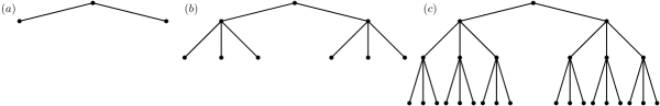
Notice that the Hasse diagram of the poset is a rooted tree with levels, where a vertex of level has precisely “children”.
For an example of posets see Figure 4.
Figure 4. Hasse diagram of posets: , , .
For integers and , let us denote by the group of automorphisms of the poset .
In the case , it is useful to consider iterated partitions of level and type together with the group of symmetries of the poset .
In fact, the group of symmetries in this case is which coincides with the natural group of symmetries of the configuration space .
This group was essentially used for identification of partitions of level and type which solve the general Nandakumar & Ramana-Rao conjecture [17], [7].
More generally, the group naturally acts on the set of partitions of level and type , and will be crucial ingredient for the configuration map – test map scheme set up in Section 2.3 to identify iterated solutions to the general Nandakumar & Ramana-Rao conjecture which are of level and type .
Definition 2.4.
Let and be integers. We define the group inductively as follows.
–
For we set .
–
For let
be the semi-direct product; for a definition of semi-direct product consult for example [11, Sec. 5.5]. The symmetric group acts on the product by
for and .
Written down in more details for , the operation in the wreath product is given inductively by
where .
Lemma 2.5.
Let and be integers. Then, there is a group isomorphism
Proof.
The proof is by induction on , becasue the definitions of relevant objects were given inductively.
For we have that .
Indeed, acts on the level one elements of by the rule for each .
Suppose now that .
By the induction hypothesis, it is enough to show the existence of an isomorphism
(11)
One way to construct an isomorphism is to map an element
by a composition of the following two maps.
(1)
The first one permutes the level one elements , together with their respective principal ideals , by the rules
for each , where the (order) ideals are mapped in the canonical way preserving the order of the indices on each level.
(2)
The second one applies the automorphism to the (order) ideal using the unique isomorphism which preserves the order of the indices, for each .
Defined in this way, the map (11) is a bijection, since each element of is uniquely determined by the permutation of its level-one elements and the automorphism of their respective principle (order) ideals.
For an illustration of the isomorphism (11) see Figure 5.
∎
Figure 5. Action of the element .
Definition 2.6.
Assume that a group acts on the set and that the symmetric group acts on the set .
Let be the semi-direct product, where acts on the product by permuting the coordinates. The induced action of on the set , given by
for each , , , and , is called the wreath product action.
2.3. Configuration Space – Test Map scheme
In the previous section we described partitions of into parts of level and type .
Hence, all such partitions are contained in the space , but is it possible to continuously parametrise them by a topological space?
In this section we first give a positive answer to the previous question, and then develop the related configuration space – test map scheme for finding solutions to Conjecture 1.2 which are of level and type .
Definition 2.7(Wreath product of Configuration Spaces).
Let and be integers.
The space is defined inductively as follows.
–
For set .
–
For let
The action of the symmetric group on the configuration space induces an action of the group on .
Let us introduce this action explicitly by induction on .
–
For the group acts on by permuting the coordinates
where and .
–
For and the group acts on the space by the rule
where
and
In similar situations, where the action is defined analogously, we will call it simply the wreath product action, in the light of Definition 2.6.
Next, for a given convex body , we define a parametrisation of the iterated equal mass convex partitions of .
Proposition 2.8(Parametrisation of iterated partitions).
Let , and be integers, and let be a -dimensional convex body. Then, there exists a continuous -equivariant map
Proof.
As already discussed in the case when is the Lebesgue measure itself, for each integer and , due to the theory of optimal transport (see [17, Sec. 2] and [7, Sec. 2]) there exists an -equivariant map
(12)
where represents the unique regular equipartition of with respect to the measure and sites . In Lemma 6.3 we provide a topological proof of the existence of the map (12).
One can consider (12) as the map given on slices and construct an -equivariant map with enlarged domain
(13)
where the symmetric group acts on the -coordinate of the domain trivially, and on the codomain by permuting the coordinates. Continuity of the map (13) is proved in Theorem 6.6, and it, in particular, implies continuity of the map (12).
We prove something a bit stronger than the statement of the proposition. Namely, we show existence of an -equivariant map
(14)
which on each slice
equals to the desired -equivariant map
from the statement of this proposition.
The -action on the -coordinate of the domain of the map (14) is trivial, and the action on the codomain of (14) is given inductively by the wreath product action (see Definition 2.6).
The construction of a map is done by induction on . For the base case , the map (13) has the desired restriction properties (12), hence we set .
Let now and set and to simplify the notation.
Assume moreover there exists an -equivariant parametrisation map
(15)
with the required slice-wise restrictions. The map is constructed from two ingredients.
(1)
Let the -equivariant map
(16)
be the product of the identity on and the map (13) with value . The action of the group on the codomain of the map (16) is induced by the product action of on , and the action of on the product which permutes the coordinates. Notice that the map (16) restricts to the slice-wise equivariant map
for each .
(2)
The -fold product of the map (15) induces the -equivariant map
(17)
From the induction hypothesis it follows that the map (17) restricts to the slise-wise equivariant map
for each .
Having these two ingredients, we can define the map (14) as the -equivariant composition
The slice-wise restrictions of the maps (16) and (17) imply that the restriction of the map factors as
for each , which finishes the proof.
∎
In order to proceed with setting up the configuration space – test map scheme, we first define an -representation which is used as a codomain of the test map of the scheme.
For each let . It will be convenient to consider to be a space of row vectors with zero coordinate sums.
Definition 2.9.
Let , and be integers.
The vector space is defined inductively as follows.
–
For set
–
For let
The dimension of the vector space in the case is .
From the inductive relation
where , it follows that
In the analogy to the case of , the action of on is defined by the wreath product action; consult Definition 2.6.
Let be the unit sphere of .
Now, we state the main theorem of this section which establishes the configuration space – test map scheme.
Theorem 2.10.
Let , and be integers.
Let be a -dimensional convex body and .
If there is no -equivariant map of the form
(18)
then there exists a solution to Conjecture 1.2 for the convex body which is of level and type .
Proof.
Let us first construct an -equivariant map
(19)
which tests whether a convex equipartition of into parts is a solution to Conjecture 1.2.
The map will be induced from the functions , which are given in the statement of the conjecture, and will be defined inductively on .
In fact, it will be given on a larger domain , where the action of the group is as before.
For , the -equivariant map
is given by mapping to the an element which, for each , has in the coordinate living in the th copy of the vector obtained from
Suppose and assume the -equivariant map
is already constructed .
We define the desired -equivariant map
by mapping an element to an element which:
–
for each , at the coordinate living in the th copy of has the value , and
–
for each , at the coordinate living in the th copy of is the vector
Here we denoted by the composition
for any integer . In the current situation .
This completes the construction of the map .
From the induction hypothesis it follows that is indeed -equivariant.
The crucial property of the map (19) is that it maps a tuple to the origin if and only if the tuple satisfies
for each .
Now, we return to the proof of the theorem.
Assume that for a convex body there is no solution to Conjecture 1.2 which is of level and type .
We will show that there exists an -equivariant map of the form (18).
Namely, since does not solve the conjecture, the -equivariant map (19) does not hit the origin.
In other words the map restricts to the map
(In order to simplify notation we do not introduce new name for the restriction.)
Pre-composing it with the -equivariant parametrisation map
from Proposition 2.8, and post-composing it with the -equivariant retraction
3. Proof of Theorem 1.3: Equivariant Obstruction Theory
In this section we give a proof of Theorem 1.3 using equivariant obstruction theory of tom Dieck [26, Sec. II.3].
Namely, for integers , and we show that an -equivariant map
does not exist if and only if are powers of the same prime number.
In order to use the equivariant obstruction theory [26, Sec. II.3], we need to construct a cellular model of the space which is also its -equivariant deformation retract.
Then, instead of studying the existence of an -equivariant map , we focus our attention on the equivalent problem of the existence of an -equivariant map
3.1. Cellular model
Blagojević & Ziegler [7, Sec. 3] have constructed an -dimensional -equivariant cellular model of the Salvetti type for the classical configuration space which is its -equivariant deformation retract.
In this section, we use this model to construct an -equivariant model of which is of dimension and is its -equivariant deformation retract.
Additionally we collect relevant facts about this model needed for an application of the equivariant obstruction theory.
For integers , and we simplify notation on occasions by setting
and .
However, we will keep the longer notation in statements of definitions, lemmas, propositions, and theorems.
Definition 3.1(Cellular model).
Let , and be integers.
An -equivariant cell complex is defined inductively as follows.
Since in the base case , it follows that the dimension of the complex is indeed
Even though depends also on parameters and , for simplicity sake they will be omitted from the notation. However, we will keep parameter in the notation, as most of the proofs are done using induction on . This convention will be kept for other notions when there is not danger of confusion.
Proposition 3.2.
Let , and be integers.
Then is a finite, regular, free -CW-complex.
Moreover, it is an -equivariant deformation retract of the wreath product of configuration spaces .
Proof.
The proof is done by induction on . For the base case let
be the -equivariant deformation retraction and the equivariant homotopy guarantied by [7, Thm. 3.13].
Here is the inclusion.
Let now .
The deformation retraction is set to be
By the induction hypothesis it follows that the complex is finite, regular and free, as well as the fact that is indeed an -equivariant retraction.
Furthermore, the homotopy defined by
makes into a deformation retraction.
Here, is the inclusion.
∎
Let us describe in more detail the cellular structure of the -CW complex developed by Blagojević & Ziegler in [7, Thm. 3.13].
The set of cells of the -CW complex complex is
The dimension if the cell is given by the formula , making the complex -dimensional.
The cellular -action is given on the cells by , for each .
In particular, from this information, we obtain the following:
–
There are in total maximal cells, all of which belong to the same -orbit.
Of special importance for later calculations will be the maximal cell , where .
Any other maximal cell is equal to .
–
There are in total codimension one cells split into orbits of the group .
For let us denote by the vector which has value on all coordinates different from , and value on coordinate . In this notation, codimension one cells are encoded by the set
For example, one choice of orbit representatives is .
Boundary of a maximal cell consists of the following codimension one cells, as can be seen either from the boundary relations in [7, Thm. 3.13] or explicitly from the proof of [7, Lem. 4.1].
For , integer , and a -element subset , let us denote by the permutation
where and is the ordering of the elements. The set of codimension one cells in the boundary of the maximal cell is encoded by the set
(20)
where two cells and belong to the same -orbit if and only if . In particular, for each , the size of the intersection of the orbit of the cell with the above set of boundary cells is precisely .
Extending the notation introduced above, let us define a generalisation of the special cell of , which was chosen to be the representative of the orbit of maximal cells.
Let , and be integers.
We define a maximal cell of the cell complex inductively as follows.
–
For let be a maximal cell in .
–
For let us define
to be a maximal cell in cell complex
where denotes the previously defined maximal cell of and is a maximal cell of .
In the next lemma we describe the index set for the codimension one cells lying in the boundary of the -cell .
Lemma 3.4.
Let , and be integers.
(i)
All maximal dimensional cells of form a single -orbit.
(ii)
The orbit representative maximal cell chosen in Definition 3.3 has the boundary consisting of codimension one cells which are indexed by the set
(iii)
The -orbit stratification of is given by
Proof.
The proof of all three statements is done simultaneously by induction on .
The base case of the complex is treated in [7, Lem. 4.1] and [7, Proof of Lem. 4.2].
See also the boundary description (20).
A codimension one boundary cell corresponds to an element
for each and with .
Let .
From the inductive definition of the cell complex and the induction hypothesis it follows that the -cells form a single -orbit, which completes the proof of part (i).
By the boundary formula of the product applied to the cell it follows that the -cells in the boundary are of the following two types.
(1)
The first type is
where and is the codimension one boundary cell of . Let be indexed by . The above -cell is set to be indexed by
From the inductive definition of the -action it follows that two boundary cells of the first type indexed by
are in the same -orbit if and only if , and cells are in the same -orbit.
(2)
The second type is
where and with . Here, denotes the codimension one boundary cell of described in (20). The above -cell is set to be indexed by
From the definition of the group action it follows that two boundary cells of the second type, indexed by non-empty proper subsets , are in the same -orbit if and only if .
In particular, we obtained a recursive formula
which together with the base case description of implies the part (ii).
Since no cell of the first type is in the same -orbit as the cells of the second type, by the above orbit description of the cells of each of the two types, it follows that the orbit stratification of stated in the part (iii) holds.
∎
3.2. Obstructions
Our goal is to show that an -equivariant map
(21)
does not exists if and only if are all powers of the same prime number.
We have that:
–
is a free -CW complex of dimension ,
–
the dimension of the -sphere is , and
–
is -simple and -connected.
Applying the equivariant obstruction theory [26, Sec. II.3], we get that the existence of an -equivariant map (21) is equivalent to the vanishing of the primary obstruction class
where is the obstruction cocycle associated to a general position equivariant map (see [4, Def. 1.5]).
Its values on the -cells are given by the following degrees
where is the radial retraction.
The Hurewicz isomorphism [8, Cor. VII.10.8] gives an -module isomorphism
The -module is isomorphic to as an abelian group.
In order to describe the -module structure on we first introduce the notion of “orientation function” as follows.
Definition 3.5.
(Orientation function)
Let , and be integers.
The orientation function
is given inductively on as follows.
–
For we set for each , where denotes the sign of the permutation.
–
For we set
for any
In the next lemma we show that the action of changes orientation on the vector space according to the orientation function .
Consequently, the -module structure on is given by
(22)
for each .
Lemma 3.6.
Let , and be integers.
The group acts on the vector space by changing the orientation according to the orientation function from Definition 3.5. In particular, the map
is a group homomorphism.
Proof.
The proof is by induction on .
The base case is treated in [7, Sec. 4, p. 69].
Indeed, each transposition acts on by reflection in the hyperplane , so a permutation reverses the orientation on by .
Thus, changes the orientation of by .
Let .
We can split the action of an element
on a vector
in two steps and as follows.
We have
In the step permutation acts on by changing the orientation by , and permutes the vectors changing the orientation by
In the step each of the elements acts on and changes the orientation by .
In total, an element acts on the vector space and changes the orientation by
∎
To evaluate the obstruction cocycle, we use the -equivariant linear projection
given by forgetting the th coordinate.
It serves as a general position map and is defined inductively as follows.
–
For the map forgets the th coordinate.
–
For we define to be the -equivariant map
Since by construction we have (see [7, Sec. 3]), by restriction of the domain we can speak of the -equivariant map
By induction on it follows that , so we may speak about the -equivariant map
Lemma 3.7.
Let , and be integers.
Then the following statements hold.
(i)
The linear map maps all -cells of by a cellular homeomorphism to the same star-shaped -neighbourhood of the origin.
(ii)
There exists an orientation of the - and -cells of the cell complex such that the cellular action of on - and -cells changes the orientation according to the orientation function defined in Definition 3.5.
(iii)
Assuming the orientations of the cells of from part (ii), the obstruction cocycle has the value on all oriented -cells of .
(iv)
Assuming the orientations of the cells of from part (ii), the following formula of cellular chains holds
where denotes the -cell in the boundary of indexed by in light of Lemma 3.4(ii) , and is a sign function constant on each -orbit.
Proof.
As usual, all statements are proved by the (same) induction on .
The base case is treated in [7, Lem. 4.1].
There, the -cells in are oriented such that they all appear with a sign in the cellular boundary formula of .
Now, assume that .
–
We define
,
where is the star-shaped neighbourhood from the induction hypothesis. Any -cell of equals to the product of maximal cells of and a maximal cell of . Therefore, by induction hypothesis and the inductive definition of the map , it follows that restricted to the cell is cellular homeomorphism.
–
Let and the -cells in be endowed with the product orientation. The map sends each - and -cell of homeomorphically to and a -cell in the boundary of , respectively. Thus, we can set orientation on each - and -cell of such that restricted to them is orientation preserving. By Lemma 3.6 the -action on changes the orientation by the sign given by orientation function , so the same is true on the cells of .
–
Since is orientation preserving cellular homeomorphism, we have
for each -cell .
–
Since is regular, we need to show only that for any in the same orbit. By the boundary of the cross-product formula for , we have the following equality of cellular -chains:
By the induction hypothesis, we have
Moreover, we have if are in the same -orbit and if are in the same -orbit. Similarly to the proof of Lemma 3.4, boundary cells of are divided into two types.
(1)
Cells of the first type are of the form
for and . By part (iii) of Lemma 3.4 or its proof, it is seen that such a cell receives a label
Moreover, two cells labeled by are in the same -orbit if and only if and are in the same -orbit. Therefore, by the inductive sign formula for the cells of the first type
the claim follows for the boundary cells of the first type.
(2)
Cells of the second type are of the form
for . Again by part (iii) of Lemma 3.4 or its proof, it is seen that such a cell receives a label . Moreover, two cells labeled by are in the same -orbit if and only if are in the same -orbit. Therefore, by the inductive sign formula for the cells of the second type
the claim follows for the boundary cells of the second type.
Finally, by part (iii) of Lemma 3.4 or its proof, no cell of the first type is in the same orbit as a cell of the second type, so the proof is completed.
∎
3.3. When is the obstruction cocycle a coboundary?
In this section we discuss when the computed cocycle is a coboundary, and consequently complete the proof of Theorem 1.3.
The orientation of cells of the complex is understood to be the one from Lemma 3.7(ii). The following lemma is a generalisation of the case treated in [7, Lem. 4.2].
Lemma 3.8.
Let , and be integers. Then the following statements hold.
(i)
The value of the coboundary of any equivariant cellular cochain
is the same on each -cell of and is equal to the -linear combination of binomial coefficients
(23)
(ii)
For any -linear combination of binomial coefficients (23), there exists a cochain whose coboundary takes precisely that value on all -cells of .
Proof.
Let
be a cellular cochain.
The group :
–
changes the orientation of any - or -cell according to the orientation function (consult Lemma 3.7 (ii)), and
–
acts on by multiplication with the value of (see (22)).
Therefore, an -module morphism of the form
is constant on each -orbit.
In particular, since -cells form a single -orbit by Lemma 3.4(i), it follows that the coboundary has the same value on all -cells.
Therefore, we restrict our attention to the orbit representative -cell introduced in Definition 3.3 and the value .
To prove part (ii), let us show that any -linear combination
is equal to the value , for some cellular -cochain . The value of can be chosen independently on each orbit. For example, one can set to be the equivariant extension of the map given on boundary cells of as
By [26, Sec. II.3] the equivariant map exists if and only if the cohomology class vanishes.
This happens if and only if is the coboundary of some equivariant cellular cochain in .
By Lemmas 3.7 and 3.8 this happens if and only if there exists a linear combination of binomial coefficients
which is equal to . This equivalent to the fact that the greatest common divisor of all such binomial coefficients equals , which by Lemma 3.9 happens if and only if are not all powers of the same prime number.
∎
In this section we give a short proof of the existence part of Theorem 1.3 using the little cubes operad structural map.
As before, let us set .
Our goal is to show the existence of an -equivariant map
in the case when are not all powers of the same prime number.
In the remainder of the section, we will consider as the subgroup of the symmetric group , where .
Indeed, is the automorphism group of the poset by Lemma 2.5.
In particular, it permutes the elements of level of .
Hence, it is a subgroup of all permutations of the level elements of , which can be identified with .
Note that this description specifies the inclusion of into .
Let denote the little cubes operad as introduced by May [18]. See also [3, Sec. 7.3] for notation.
Each is a free -space. The operad comes with the structural map
for any integers and .
Moreover, we have the following fact [18, Thm. 4.8].
Lemma 4.1.
Let and be integers. Then, is -homotopy equivalent to the configuration space .
The special case of the structural map when is useful for us, as explained in the following lemma, consult also [3, Lem. 7.2].
Lemma 4.2.
Let and be integers. The structural map
is -equivariant. The action of on the domain is assumed to be the wreath product action from Definition 2.6, and the action on the codomain is given by restriction .
Now, we prove the following auxiliar result.
Lemma 4.3.
Let , and be integers.
There exists an -equivariant map
where and the action on the codomain is the restriction action .
Proof.
We will show the existence of an -equivariant map
by induction on .
The base case the map is the equality.
Assume .
As before, let and .
The map is defined by the following diagram:
The group acts on by the wreath product action induced from , so the top horizontal map is -equivariant by the induction hypothesis.
Both vertical maps are -equivariant by Lemma 4.1.
Indeed, the left one is the product of equivariant homotopy equivalences, hence its homotopy inverse is equivariant as well. Finally, the bottom horizontal map is -equivariant by Lemma 4.2.
∎
Next, we prove an additional auxiliar result.
Lemma 4.4.
Let , and be integers. Then, there exists an -module monomorphism
where and the action on the codomain is the restriction action .
Proof.
Since we have it is enough to show there exists an -equivariant monomorphism
We will prove this by induction on .
In the base case we set to be the identity.
Assume .
Let and . It is enough to show there exists an -equivariant monomorphism of the form
(25)
where acts on the codomain by the wreath product action from Definition 2.6 and acts on by the restriction .
Indeed, then the desired map can be set to be the -equivariant composition
Finally, the map (25) can be constructed as follows.
Let
where .
Furthermore, let us denote by
–
the average of the coordinates of the vector for each , and
–
the average of the coordinates of the vector .
With this notation, we have that
for each , as well as
Finally, we set the map (25) to be such that it sends to the vector
This map is injective. Moreover, the restriction action on and the wreath product action of on make it -equivariant.
∎
Finally, we give the second proof of the existence part of Theorem 1.3.
Let , and be integers.
Assume that are not all powers of the same prime number. Then, there exists an -equivariant map
Proof.
If are not all powers of the same prime number, in particular is not a power of a prime number, hence by [7, Thm. 1.2] there exists an -equivariant map
Let us set . Precomposing this map with the map from Lemma 4.3 and postcomposing with the monomorphism from Lemma 4.4 we get an -equivariant composition
In this section we give yet another short proof of the existence of an -equivariant map
(26)
when are not all powers of the same prime number.
We rely on the equivariant obstruction theory, as presented by tom Dieck [26, Sec. II.3], and appropriate a trick developed by Özaydin in [22].
Let and as before.
Not that
–
is a free -cell complex of dimension , and
–
the -sphere is -simple and -connected.
Consequently, an -equivariant map (27) exists if and only if the primary obstruction
vanishes.
Here,as before, denotes the coefficient module.
In same way, for any subgroup , the existence of a -equivariant map
(27)
is equivalent to the vanishing of the obstruction class
which in particular is the restriction of the class .
For each integer and a prime number , let us fix a -Sylow subgroup . For more details on Sylow subgroups, see for example [11, Sec. 4.5].
Definition 5.1.
Let and be integers. For a prime number , let us define a subgroup inductively as follows.
(i)
For we set .
(ii)
Assume . Then, we define
Notice that is indeed a -Sylow subgroup.
For this follows from definition, while for the recursive formula
implies that the order is the maximal power of which divides the order of .
Lemma 5.2.
Let , and be integers and let be a prime number.
If are not all powers of , then the obstruction class
vanishes.
Proof.
Assume are not all powers of a prime . Let us show that the action of the -Sylow subgroup on the sphere has a fixed point.
This would produce a (constant) -equivariant map
Hence, from the discussion at the beginning of this section, we would have that .
Since
is an -equivariant deformation retract, it is enough to show that has a nonzero fixed point in the vector space . We prove this fact by induction on .
(i)
If , then is not a power of . Thus, the -Sylow subgroup does not act transitively on the set . Consequently, fixes some nonzero vector , and hence it fixes as well.
(ii)
Assume . We distinguish two cases.
(a)
The number is not a power of . Then by (i) we know that fixes a nonzero point , so the nonzero point
is fixed by .
(b)
The numbers are not all powers of . Then, by induction hypothesis, there is a nonzero vector fixed by , so the nonzero vector
is fixed by .
This completes the proof of the lemma.
∎
Now, we give the third proof of the existence part of Theorem 1.3.
The set of convex bodies in with non-empty interior is a metric space with Hausdorff metric given by
Symmetric difference metric on , given by
where is the Lebesgue measure on , induces the same topology on (see [14]). Hence convergence of a sequence in one metric is equivalent to convergence in another.
We start with the definition of the generalised Voronoi diagram.
Definition 6.1.
For and let us denote by
the generalised Voronoi diagram with sites and weights , where
(29)
denotes the the Voronoi cell, for each .
Region can be considered as the set of points where the affine function
takes minimal value among all functions of the same type. In particular, regions have disjoint interiors and cover the whole .
Notice that for any , so we will usually restrict our attention to weights .
Definition 6.2.
For a convex body , sites and weights , let us denote by
the partition of given by for each .
As before, for and a probability measure on which is absolutely continuous with respect to the Lebesgue measure, let denote the space of equal mass partitions of with respect to the measure .
Let and be integers, a vector with . Let be a convex body, and let be a probability measure on which is absolutely continuous with respect to the Lebesgue measure. For any choice of sites there exist unique weights such that the generalised Voronoi diagram produces a partition of
such that
for each .
In particular, for the unique weight vector we have
The relevant case for this paper is when .
Then, the equal mass partition of a convex body with respect to guaranteed by the previous lemma is called the regular equipartition of with sites .
In [17, Sec. 2] and [7, Sec. 2] the existence of unique weights from the lemma is proved via the theory of optimal transport.
We include a topological proof of this fact developed by Moritz Firsching, which relies on some results from [12].
Let us denote by the standard basis vectors, and let be the standard -dimensional simplex.
The faces of are convex sets of the form for .
The first part of the proof of Lemma 6.3 is the following lemma.
Lemma 6.4.
Let be a continuous self map of the simplex. Then, the following statements hold.
(i)
Map is surjective if holds for all faces .
(ii)
Map is injective on the preimage of the interior if additionaly the following condition holds:
For a non-empty subset , a point , , and
Then, for every , every non-empty subset , every and every index we have such that for at least one index the inequality is strict, where denotes the th coordinate function of .
Proof due to M. Firsching.
(i) The map is homotopic to the identity via for . Each map in the homotopy satisfies and hence induces a homotopy of quotient maps
Since , the is not nullhomotopic and hence is surjective, since every non-surjective self map of the sphere is necessarily nullhomotopic. The surjectivity of the quotient map implies the surjectivity of by the fact that is dense in .
(ii) The injectivity argument is similar to the one in [12, Thm. 1]. Suppose for two different points we have . Then , since maps each face to iteself. Define
Since we have . We will inductively define a sequence of points
for some integer , which satisfy
and such that for each we have for all , with the strict inequality holding true for at least one index in . Indeed, if we prove this, than for the index for which the strict inequality is achieved, we would have
which contradicts .
Suppose with the above properties have already been constructed, for some , and let us construct . Since , by the assumption of part (ii), there exists some with
such that the point satisfies and for all , with the strict inequality for at least one index . If , then and , so we stop induction. Otherwise, we continue for finite more steps until .
Let us fix a point . We want to show existence of a weight vector .
Given a point set
.
Here we allow and extend the definition of to include weight vectors with some (but not all) coordinates being .
We define the continuous map by
If this map is surjective and injective on the preimage , we can set , where is the unique point in the fiber of . To prove the property of the map we use Lemma 6.4.
Before doing that, let us see why the map is continuous.
First, notice that if we show it is continuous on the interior , the continuity of on the whole domain follows by density of the interior and the fact that the value of on the boundary is the limit value of interior points.
Thus, let as be a convergence in .
Then by part (ii) of Lemma 6.7 for each we have
To prove surjectivity of , by Lemma 6.4 part (i) it is enough to show that maps each face to itself. Indeed, assume for we have for some . Then the th coordinate of is and the th coordinate of is zero, since the th Voronoi region is empty.
Therefore a face of is mapped to itself by .
For injectivity of on the preimage we use Lemma 6.4 part (ii). We want to show that for any point , nonempty , and the condition in part (ii) is satisfied. Notice that the coordinate function of satisfies
for and
If we denote by the weight vector obtained from by adding a constant
to each coordinate, we have equality of Voronoi diagrams
so one can use the weight vector to calculate .
Moreover, we have
for and for . In particular, for each we have
which implies . Therefore, by [12, Lem. 2] it follows that there exists an index such that . Hence, the assumption in part (ii) of Lemma 6.4 holds.
∎
6.2. Continuity of partitions
Lemma 6.3 implies that, for a given , the function
exists and is -equivariant. In [15, Lem. 3] it was shown that the function is continuous on parameter .
Since the function also depends on the convex body it is natural to ask: Is the fuctnion continuous in parameters ?
We give the positive answer to this question in the lemma which follows.
For the proof see Section 6.3.
Lemma 6.5(Continuity of weights).
Let be a probability measure on which is absolutely continuous with respect to the Lebesgue measure. The assignment
given by Lemma 6.3, is continuous and -equivariant, where the -action on the -coordinate in the domain is set to be trivial.
For a given convex body , the continuity of the assignment
given by Lemma 6.3, is proved in [17, Thm. 2.1] and [7, Thm. 2.1].
Again as before, this assignment depends on , so the next natural question arises: Is continuous in parameters ?
The main result of this section is the following theorem which gives the positive answer to the previous question.
Theorem 6.6(Continuity of partitions).
The function
where is the regular partition of with sites from Lemma 6.3, is a continuous -equivariant map which satisfies the restriction property
for each .
Proof.
To show the claim, it is enough to show that for each the coordinate map
is continuous, where weights are given by Lemma 6.3, and region is the th component (29) of the generalised Voronoi diagram with sites and weights .
To show sequential continuity, let
be a converging sequence, and let us denote the weights by and .
By Lemma 6.5, we have as .
Moreover, since has a non-empty interior and as , it follows that
has a non-empty interior as well, hence .
Therefore, all notions used in the following string of inequalities are well defined. We have
because the first summand in the last row tends to zero as by Lemma 6.7 (ii), so the continuity follows.
∎
6.3. Auxiliar lemmas
For a vector such that let us denote by
the affine hyperplane induced by , and by
the corresponding closed half-space.
Lemma 6.7.
Let . Then, the following statements are true.
(i)
Assume the convergence
with , as well as
for each . Then
as .
(ii)
Assume the convergence
and let , as well as
for each . Then
as .
Proof.
(i)
Since and induce the same topology on , it is enough to prove convergence in metric.
Recall that
For the first supremum we have
Indeed, assume to the contrary that for some sequence , we have that
Since is compact, we could have chosen the sequence from the very start such that , and so
From this we obtain a contradiction by showing for . This is indeed true, since
For the second supremum we have that
Indeed, assume to the contrary that for some sequence we have
Since is compact, there is a subsequence with , hence
for each . Notice first that . Indeed, strict inequality would
which would mean , which is impossible. Since by assumption, by convexity there exists
with . Moreover, we have for , since
This means that
for , which is a contradiction.
(ii) We will first show that for two converging sequences and in such that , we have
as . Indeed, from
it follows that
as desired.
Back to the proof of the main claim. For and the th component of the generalised Voronoi diagram is equal to the intersection of closed half-spaces
for and . Therefore, by the repeated use of the above intersection argument and part (i), we have
which completes the proof.
∎
Recall, for a measure which is absolutely continuous with respect to the Lebesgue measure on , by the Radon-Nikodym theorem, there exists an integrable function such that
for each measurable set . We will need the next measure-theoretic claim.
Lemma 6.8.
Let be a probability measure on which is absolutely continuous with respect to the Lebesgue measure . Then, the following implication holds
(30)
where is any sequence of measurable sets in .
Proof.
The proof, in essence, follows from a use of the Dominant Convergence Theorem [1, Sec. A3.2].
Let denotes the characteristic function of a measurable set .
We prove (30) in two steps.
Let is first show that a sequence of functions converges pointwise almost everywhere to the zero function. Indeed, let denote the pointwise limit of the sequence . Let and let us restrict to a subsequence such that
.
Then, we have
and therefore
Since this holds for any , it follows that , so is zero almost everywhere.
Finally, by the Dominant Convergence Theorem applied to the dominant , we have
which finishes the proof of the implication (30).
∎
Let us shorten the notation and denote and for each .
First, notice that the sequence is bounded. Indeed, as implies
so bodies are contained in a bounded region around . Similarly, as implies that the sites live in a bounded region around . Therefore, for any the difference must be bounded for all , proving that the sequence is bounded in . Indeed, if for some we have as , it would imply
for , which is a contradiction.
Convergence as is equivalent to the same convergence for each subsequence of . Let us assume the latter is not true and seek a contradiction. By the boundedness of weights, and after possibly restricting to a subsequence, we have as , for some . Due to the uniqueness of the weight vector in for given sites and a convex body , contradiction would follow from the fact that
[1]
Hans Wilhelm Alt, Linear functional analysis, Universitext,
Springer-Verlag London, Ltd., London, 2016, An application-oriented
introduction, Translated from the German edition by Robert Nürnberg.
[2]
Imre Bárány, Pavle Blagojević, and András Szűcs,
Equipartitioning by a convex 3-fan, Adv. Math. 223 (2010),
no. 2, 579–593.
[4]
Pavle V. M. Blagojević and Aleksandra S. Dimitrijević Blagojević,
Using equivariant obstruction theory in combinatorial geometry,
Topology Appl. 154 (2007), no. 14, 2635–2655.
[5]
Pavle V. M. Blagojević, Wolfgang Lück, and Günter M. Ziegler,
Equivariant topology of configuration spaces, J. Topol. 8
(2015), no. 2, 414–456.
[6]
Pavle V. M. Blagojević and Pablo Soberón, Thieves can make
sandwiches, Bull. Lond. Math. Soc. 50 (2018), no. 1, 108–123.
[7]
Pavle V. M. Blagojević and Günter M. Ziegler, Convex
equipartitions via equivariant obstruction theory, Israel J. Math.
200 (2014), no. 1, 49–77.
[8]
Glen E. Bredon, Topology and Geometry, Graduate Texts in Math., vol.
139, Springer, New York, 1993.
[9]
Frederick R. Cohen, The homology of -spaces, , in: “The Homology of Iterated Loop Spaces”, Lecture Notes in
Mathematics, vol. 533, Springer-Verlag, Heidelberg, 1976, pp. 207–351.
[10]
Albrecht Dold, Simple proofs of some Borsuk-Ulam results,
Proceedings of the Northwestern Homotopy Theory Conference
(Evanston, Ill., 1982), Contemp. Math., vol. 19, Amer. Math. Soc.,
Providence, RI, 1983, pp. 65–69.
[11]
David S. Dummit and Richard M. Foote, Abstract algebra, third ed., John
Wiley & Sons, Inc., Hoboken, NJ, 2004.
[12]
Darius Geiß, Rolf Klein, Rainer Penninger, and Günter Rote,
Optimally solving a transportation problem using Voronoi diagrams,
Comput. Geom. 46 (2013), no. 8, 1009–1016.
[13]
Michail Gromov, Isoperimetry of waists and concentration of maps, Geom.
Funct. Anal. 13 (2003), no. 1, 178–215.
[14]
Peter M. Gruber and Petar Kenderov, Approximation of convex bodies by
polytopes, Rend. Circ. Mat. Palermo (2) 31 (1982), no. 2, 195–225.
[15]
Alfredo Hubard and Boris Aronov, Convex equipartitions of volume and
surface area, preprint, October 2010, 9 pages; version 3, September 2011, 17
pages, http://arxiv.org/abs/1010.4611.
[16]
Roman Karasev, Equipartition of several measures, preprint, November
2010, 6 pages; version 6, August 2011, 10 pages,
http://arxiv.org/abs/1011.4762.
[17]
Roman Karasev, Alfredo Hubard, and Boris Aronov, Convex equipartitions:
the spicy chicken theorem, Geom. Dedicata 170 (2014), 263–279.
[18]
J. Peter May, The geometry of iterated loop spaces, Lecture Notes in
Mathematics, Vol. 271, Springer-Verlag, Berlin-New York, 1972.
[19]
Yashar Memarian, On Gromov’s waist of the sphere theorem, J. Topol.
Anal. 3 (2011), no. 1, 7–36.
[21]
R. Nandakumar and N. Ramana Rao, Fair partitions of polygons: an
elementary introduction, Proc. Indian Acad. Sci. Math. Sci. 122
(2012), no. 3, 459–467.