Performance improvement of a fractional quantum Stirling heat engine

Abstract

To investigate the impact of fractional parameter on the thermodynamic behaviors of quantum systems, we incorporate fractional quantum mechanics into the cycle of a quantum Stirling heat engine and examine the influence of fractional parameter on the regeneration and efficiency. We propose a novel approach to control the thermodynamic cycle that leverages the fractional parameter structure and evaluates its effectiveness. Our findings reveal that by tuning the fractional parameter, the region of the cycle with the perfect regeneration and the Carnot efficiency can be expanded.

I Introduction

The study of fractional calculus (Herrmann, 2011; Kilbas et al., 1993; Butzer and Westphal, 2000) has received growing attention in recent years due to its unique mathematical structure and close association with the renormalization and the inverse power law. It provides a powerful mathematical tool to solve problems related to complex systems (West, 2014; Guo et al., 2021). In addition, Lévy flight, a natural generalization of Brownian motion, has become a research hotspot in the field of anomalous diffusion with practical implications for the advancements of physics, life science, information science, and other disciplines (Khinchine and Lévy, 1936; Mandelbrot and Mandelbrot, 1982; de Jager et al., 2011; Zaburdaev et al., 2015; Barthelemy et al., 2008; Margolin and Barkai, 2005; Liu et al., 2016). Lévy flight arises from the strong interaction between particles and their environment, and it is a Markov stochastic process characterized by long-range jumps. Although the Lévy process is mainly utilized for numerical simulations, the experimental work (Sagi et al., 2012) has shown that it is feasible to adjust the system parameters with precision, enabling direct experimental studies of Lévy flight. Hence, discussions on the diffusion behavior and the dynamics of atomic groups with damping and even more complex transport environments are underway.

Applications of fractional quantum mechanics have been developed by defining the fractional path integral over Lévy paths and using the Riesz fractional derivative, extending the concept of fractality in quantum physics (Laskin, 2000a, b, c, 2002, 2018). This area has witnessed significant advances in recent years (Naber, 2004; Wang and Xu, 2007; Dong and Xu, 2008; Felmer et al., 2012; Secchi, 2013; Fall et al., 2015; Wei, 2015; Longhi, 2015; Laskin, 2017), and has been demonstrated experimentally (Liu et al., 2023). Moreover, fractional calculus is increasingly being employed to describe thermodynamic phenomena (Mainardi, 1997; Tudor and Viens, 2007; Wang et al., 2014; Meilanov and Magomedov, 2014; Bagci, 2016; Lopes and Machado, 2020; Tarasov, 2006; Sisman and Fransson, 2021; Khadem et al., 2022; Korichi et al., 2022). Attempts have also been made to combine fractional quantum mechanics with thermodynamics, such as Black hole thermodynamics (Jalalzadeh et al., 2021), thermal properties of fractional quantum Dirac oscillators (Korichi et al., 2022), and etc.

Quantum heat engine (Scovil and Schulz-DuBois, 1959; Geusic et al., 1967; Quan et al., 2005; Kieu, 2006; Quan et al., 2007; Wu et al., 1998; Huang et al., 2014) is an excellent platform for studying the thermodynamic properties of quantum systems. In this context, we investigate the effect of the fractional parameter on the performance of a quantum Stirling engine (QSE). We propose a new thermodynamic process based on the fractional parameter and analyze the behavior of the thermodynamic cycle that incorporate this process. It will demonstrate the potential applications of fractional quantum mechanics in thermodynamics.

This paper is organized as follows: In Section II, we provide a brief overview of fractional quantum mechanics and show the solution in the infinite potential well (IPW). Several fundamental concepts of quantum thermodynamics are introduced as well. In Section III, we introduce the structure of the QSE and propose a new way to regulate the thermodynamic cycle based on fractional parameters. Expressions of thermodynamic quantities in the cycle are provided. In Section IV, the effects of the fractional parameter on the performance of the QSE are discussed. Conclusions are given in Section V.

II FRACTIONAL QUANTUM MECHANICS AND KEY quantities IN QUANTUM THERMODYNAMIC PROCESSES

II.1 FRACTIONAL QUANTUM MECHANICS

In fractional quantum mechanics, the fractional Hamiltonian operator is defined as $H=D_{\alpha}|p|^{\alpha}+V(x)\text{,}$ where $p$ is the momentum, the fractional parameter $1<\alpha\leq 2$, $V(x)$ is the potential energy as a functional of a particle path $x$ , and $D_{\alpha}$ is the scale coefficient (Laskin, 2000a; Korichi et al., 2022). If the system at an initial time $t_{a}$ starts from the point $x_{a}$ and goes to the final point $x_{b}$ at time $t_{b}$, one could define the quantum-mechanical amplitude, often called a kernel, $K\left(x_{b}t_{b}\mid x_{a}t_{a}\right)$. The kernel function is the sum of the contributions of all trajectories through the first and last points (Laskin, 2000a, b, c, 2002, 2018). The kernel based on the Lévy path in phase space is defined as

$$K\left(x_{b}t_{b}\mid x_{a}t_{a}\right)=\lim_{N\rightarrow\infty}\int_{-\infty}^{\infty}dx_{1}\ldots dx_{N-1}\frac{1}{(2\pi\hbar)^{N}}$$ (1)

$$\times\int_{-\infty}^{\infty}dp_{1}\ldots dp_{N}\exp\left\{\frac{i}{\hbar}\sum_{j=1}^{N}p_{j}\left(x_{j}-x_{j-1}\right)\right\}$$

$$\times\exp\left\{-\frac{i}{\hbar}D_{\alpha}\varepsilon\sum_{j=1}^{N}\left|p_{j}\right|^{\alpha}-\frac{i}{\hbar}\varepsilon\sum_{j=1}^{N}V\left(x_{j}\right)\right\},$$

where $\hbar$ is Planck’s constant, $\varepsilon=\left(t_{b}-t_{a}\right)/N$, $x_{j}=x\left(t_{a}+j\varepsilon\right)$, $p_{j}=p\left(t_{a}+j\varepsilon\right)$, $x\left(t_{a}+j\varepsilon\right)_{j=0}=x_{a}$, and $x\left(t_{a}+j\varepsilon\right)_{j=N}=x_{b}$.

The kernel describes the evolution of a system, leading to the fractional wave function at time $t_{b}$

$$\psi\left(x_{b},t_{b}\right)=\int_{-\infty}^{\infty}dx_{a}K\left(x_{b}t_{b}\mid x_{a}t_{a}\right)\psi\left(x_{a},t_{a}\right),$$ (2)

with $\psi\left(x_{a},t_{a}\right)$ being the fractional wave function of the initial state. The fractional wave function $\psi\left(x,t\right)$ satisfies the fractional Schrödinger equation (Appendix A)

$$i\hbar\frac{\partial\psi(x,t)}{\partial t}=-D_{\alpha}(\hbar\nabla)^{\alpha}\psi(x,t)+V(x)\psi(x,t),$$ (3)

where the quantum Riesz fractional derivative $(\hbar\nabla)^{\alpha}$ is defined as

$$(\hbar\nabla)^{\alpha}\psi(x,t)=-\frac{1}{2\pi\hbar}\int_{-\infty}^{\infty}dp\>\text{exp}\left(i\frac{px}{\hbar}\right)|p|^{\alpha}\varphi(p,t)$$ (4)

with $\varphi(p,t)=\int_{-\infty}^{\infty}dp\>\text{exp}\left(-i\frac{px}{\hbar}\right)\psi(x,t)$ being the Fourier transform of $\psi(x,t)$.

In the following discussion, the scale coefficient $D_{\alpha}$ is set to be equal to $\left(1/2m\right)^{\frac{\alpha}{2}}$ with $m$ being the mass of the quantum mechanical particle (Korichi et al., 2022). For $\alpha=2$, it becomes the standard quantum mechanics that we know. Meanwhile, we consider a particle in a one-dimensional IPW, where the potential field

$$V(x)=\begin{cases}0&-L/2\leqslant x\leqslant L/2,\\ \infty&\mathrm{otherwise.}\end{cases}$$ (5)

The solution of Eq. (3) is related to the time independent wave function $\phi(x)$ by

$$\psi(x,t)=\exp\left\{-i\frac{Et}{\hbar}\right\}\phi(x),$$ (6)

where $E$ represents the energy of the particle. Putting Eq. (6) into Eq. (3) leads to the following time-independent fractional Schrödinger equation

$$-D_{\alpha}(\hbar\nabla)^{\alpha}\phi(x)+V(x)\phi(x)=E\phi(x).$$ (7)

By using Eqs. (5) and (7) and considering the boundary conditions, the eigenvalue $E_{n}\left(L,\alpha\right)$ of the fractional Hamiltonian operator $H$ and the corresponding wave function $\phi(x)$ read (Laskin, 2000b)

$$E_{n} \left(L,\alpha\right)=D_{\alpha}\left(\frac{2\pi\hbar}{L}\right)^{\alpha}n^{\alpha}$$ (8)

$$=\left(\frac{1}{2m}\right)^{\frac{\alpha}{2}}\left(\frac{2\pi\hbar}{L}\right)^{\alpha}n^{\alpha},$$

$$\phi(x)=\begin{cases}\sqrt{\frac{2}{L}}\cos\left[\left(n-\frac{1}{2}\right)\frac{2\pi x}{L}\right]&\mathrm{for\>\mathit{n\>}even\text{,}}\\ \sqrt{\frac{2}{L}}\sin\frac{2n\pi x}{L}&\mathrm{for\>}n\>\mathrm{odd},\end{cases}$$ (9)

where $L$ represents the width of the potential well, and $n$ is a positive integer $(n=1,2,3,4,...)$.

II.2 KEY QUANTITIES IN QUANTUM THERMODYNAMIC PROCESSES

The internal energy $U$ of the particle is expressed as the ensemble average of the fractional Hamiltonian operator, i.e.,

$$U=\langle H\rangle=\sum_{n}P_{n}E_{n},$$ (10)

where $P_{n}$ denotes the occupation probability of the $n$th eigenstate with energy $E_{n}$. During an infinitesimal process, the time differential of the internal energy

$$dU=\sum_{n}\left(E_{n}dP_{n}+P_{n}dE_{n}\right).$$ (11)

According to the first law of thermodynamics, $dU$ is associated with the heat $\mkern 3.0mu\mathchar 22\relax\mkern-12.0mudQ$ absorbed from the environment and the work $\mkern 3.0mu\mathchar 22\relax\mkern-12.0mudW$ performed by the external agent, i.e.,

$$dU=\mkern 3.0mu\mathchar 22\relax\mkern-12.0mudQ+\mkern 3.0mu\mathchar 22\relax\mkern-12.0mudW.$$ (12)

For the isothermal and isochoric processes, the heat exchange and the work done during an infinitesimal thermodynamic process are, respectively, identified as (Quan et al., 2005; Kieu, 2006; Quan et al., 2007; Su et al., 2018)

$$\mkern 3.0mu\mathchar 22\relax\mkern-12.0mudQ=\sum_{n}E_{n}dP_{n},$$ (13)

and

$$\mkern 3.0mu\mathchar 22\relax\mkern-12.0mudW=\sum_{n}P_{n}dE_{n}.$$ (14)

As the isothermal process with the temperature $T$ of the particle being a constant is reversible, Eq. (13) is equivalent to

$$\mkern 3.0mu\mkern 3.0mu\mathchar 22\relax\mkern-12.0mudQ=TdS,$$ (15)

where

$$S=-k_{B}\sum_{n}P_{n}\ln P_{n}$$ (16)

indicates the entropy of the particle, $k_{B}$ is Boltzmann’s constant, and

$$P_{n}=\exp\left(-\beta E_{n}\right)/\text{Tr}\left[\exp(-H/\left(k_{B}T\right))\right]$$ (17)

describes the occupation probability of a Gibbs state at energy $E_{n}$. In the next section, the theory of fractional quantum mechanics and the concepts of heat and work in quantum thermodynamic processes will be applied to build quantum engines.

III QUANTUM STIRLING ENGINE based on fractional quantum mechanics

Generally, the Stirling heat engine consists of two isothermal processes and two isochoric processes(Chen, 1997; Chen et al., 1998; Wu et al., 1998; Huang et al., 2014). We focus on revealing the necessary conditions for the perfect regeneration and the reversible operation based on fractional quantum mechanics. For this reason, the fractional isothermal process, where the fractional parameter and the well width are changed slowly, is proposed. This process can be used to construct the fractional QSE, which consists of two fractional isothermal processes $(A\rightarrow B$ and $C\rightarrow D)$ and two quantum isochoric processes $(B\rightarrow C$ and $D\rightarrow A)$, as depicted in Fig. 1. The fractional parameter provides us with a new way to regulate the thermodynamic cycle.

At stage I (A-B), the particle confined in the IPW interacts with the hot bath at temperature $T_{h}$. The fractional parameter slowly changes from $\alpha_{2}$ to $\alpha_{1}$ and the IPW varies from $L_{A}$ to $L_{B}$. The process is infinitely slow, allowing the particle to continually be in thermal equilibrium with the hot bath. The probability of each eigenstate, which has the form of Eq. (17), changes from $P_{n}^{A}$ to $P_{n}^{B}$. With the help of Eq. (15), the heat absorbed from the hot bath is written as

$$Q_{AB}=T_{h}[S(B)-S(A)],$$ (18)

where $S(i)$ is the entropy of the particle at state $i$ calculated by Eq. (16).

At stage II (B-C), the particle with the initial probability $P_{n}^{B}$ of each eigenstate is placed in contact with the the regenerator and undergoes an isochoric process until reaching the temperature $T_{c}$. The probability of each eigenstate changes from $P_{n}^{B}$ to $P_{n}^{C}$. The eigenvalue $E_{n}$ of the fractional Hamiltonian operator $H$ is kept fixed as the well width and fractional parameter maintain constant values, i.e., $L_{B}$ and $\alpha_{1}$, respectively. The temperature of the particle decreases from $T_{h}$ to $T_{c}$. There is heat exchange between the particle and the regenerator and no work is performed in this isochoric process. According to Eq. (13), the amount of the heat absorbed in this process is equal to the change of the internal energy of the particle, i.e.,

$$Q_{BC}=U\left(C\right)-U\left(B\right)=\sum_{n}E_{n}\left(L_{B},\alpha_{1}\right)\left(P_{n}^{C}-P_{n}^{B}\right),$$ (19)

where $U(i)$ is the internal energy of the particle at state $i$ calculated by Eq. (10). As $Q_{BC}<0$, heat is released to the regenerator without any work being done.

At stage III (C-D), the particle is brought into contact with the cold bath at temperature $T_{c}$. It is an isothermal process, which is a reversed process of stage I. The state of the particle is always in thermal equilibrium with the cold bath, while the fractional parameter slowly changes from $\alpha_{1}$ to $\alpha_{2}$ and the IPW varies from $L_{C}$ to $L_{D}$. Similar to Eq. (18), the heat absorbed from the cold bath is

$$Q_{CD}=T_{c}[S(D)-S(C)].$$ (20)

At stage IV (D-A), the particle is removed from the cold bath and goes through another isochoric process by connecting the the regenerator until reaching the temperature $T_{h}$, where the well width and fractional parameter are invariant. The cycle ends until the temperature of the particle increasing to $T_{h}$. Heat absorbed from the regenerator at this stage is computed by

$$Q_{DA}=U\left(A\right)-U\left(D\right)=\sum_{n}E_{n}\left(L_{A},\alpha_{2}\right)\left(P_{n}^{A}-P_{n}^{D}\right).$$ (21)

Note that $L_{D}=L_{A}$ is required for completing one cycle.

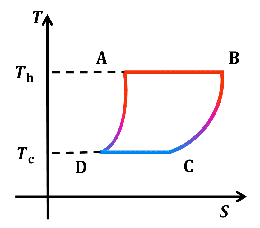
Figure 1: Temperature-entropy (T-S) diagram for a quantum Stirling engine (QSE).

As the energy contained in the particle always returns to its initial value. The net work done by the heat engine would then be

$$W=Q_{AB}+Q_{BC}+Q_{CD}+Q_{DA}.$$ (22)

The Stirling heat engine is known as a closed-cycle regenerative heat engine. The net heat exchange between the particle and the regenerator during the two isochoric processes is

$$Q_{R}=Q_{BC}+Q_{DA}.$$ (23)

Three possible cases exists: (a) $Q_{R}=0$, (b) $Q_{R}<0$, and (c) $Q_{R}>0$. The case $Q_{R}=0$ means that the regenerator is a perfect regenerative heat exchanger. The mechanism of the perfect regeneration makes the efficiency of the engine attain the Carnot value. When $Q_{R}\text{<}0$, the heat $\left|Q_{BC}\right|$ flowing from the particle to the regenerator in one regenerative process is larger than its counterpart $Q_{DA}$ flowing from the regenerator to the working substance in the other regenerative process. The redundant heat in the regenerator per cycle must be timely released to the cold bath. When $Q_{R}\text{>}0$, the amount of $\left|Q_{BC}\right|$ is smaller than $Q_{DA}$. The inadequate heat in the regenerator must be compensated from the hot bath, otherwise the regenerator may not be operated normally. Due to the non-perfect regenerative heat, the net heat absorbed from the hot bath per cycle may be different from $Q_{h}$ and is given by

$$Q_{h}=Q_{AB}+H\left(Q_{R}\right)Q_{R},$$ (24)

where $H(x)$ is the Heaviside step function. The efficiency is an important parameter for evaluating the performance, which is often considered in the optimal design and theoretical analysis of heat engines.

By using Eqs. (22) and (24), the expression of the efficiency of the QSE should be

$$\eta=\frac{W}{Q_{h}}=\frac{W}{Q_{AB}+H\left(Q_{R}\right)Q_{R}}.$$ (25)

IV resultS and discussion

By using the model presented above, the performance of the QSE through different ways of regulation will analyzed. Firstly, the QSE can be regulated by adjusting the widths of the IPW for a given fractional parameter value. Secondly, the fractional parameter can be adjusted to identify the condition for perfect regeneration in the QSE when the width of the IPW is fixed. Finally, the performance of the QSE can be improved by simultaneously adjusting both the widths of the IPW and the fractional parameters.

IV.1 THE EFFECTS OF WELL WIDTHS

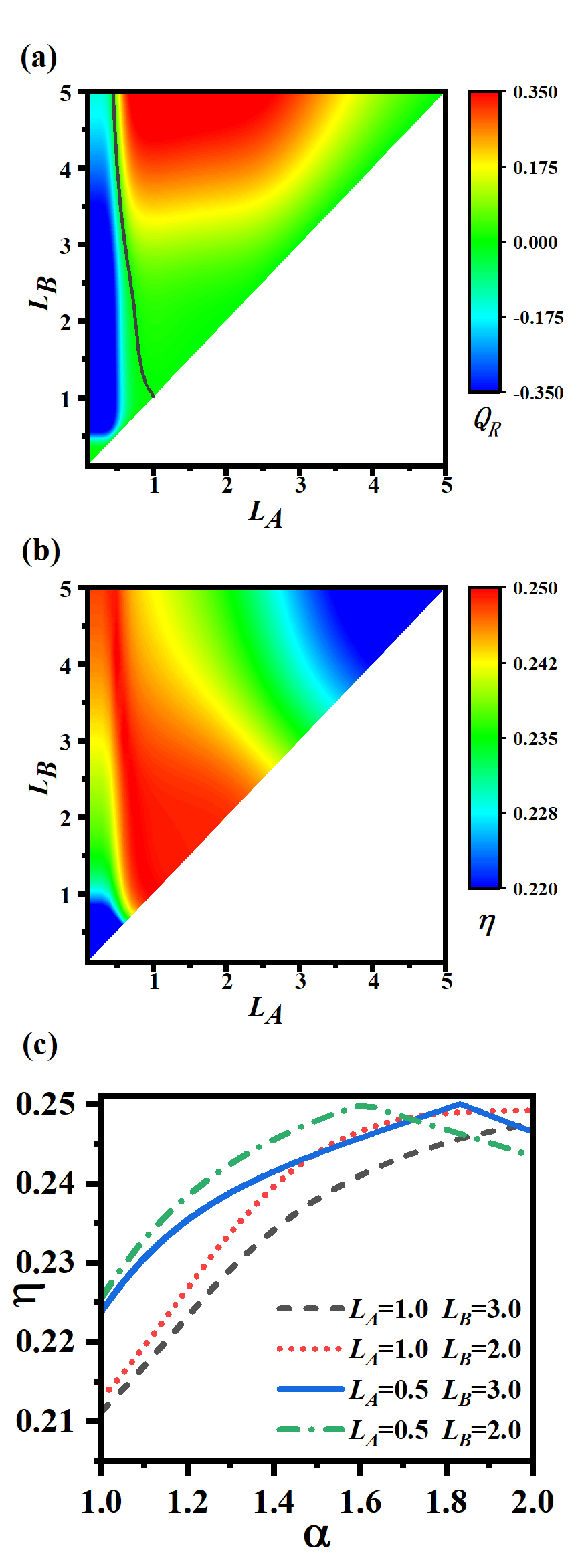
Figure 2: The contour plots of (a) the net heat exchange $Q_{R}$ between the particle and the regenerator and (b) the efficiency $\eta$ varying the widths $L_{A}$ and $L_{B}$ of the IPW, where $\alpha_{1}=\alpha_{2}=2$. The black line represents the cycle with the perfect regeneration, i.e., $Q_{R}=0$. (c) The efficiency $\eta$ of the Stirling cycle as a function of the fractional parameter $\alpha$ for $L_{B}=L_{C}=2$ (dotted line and dash-dotted line) and $3$ (solid line and dashed line), where $\alpha=\alpha_{1}=\alpha_{2}$, and $L_{A}=L_{D}=0.5$ and $1$, respectively. The parameters $T_{h}=4$, $T_{c}=3$, and $m=1$. Note that Planck’s constant $\hbar$ and Boltzmann’s constant $k_{B}$ are set to be unity throughout the paper, i.e., $\hbar=k_{B}=1$.

Fig. 2(a) shows the contour plot of the net heat exchange $Q_{R}$ between the particle and the regenerator of the QSE varying with the widths $L_{A}$ and $L_{B}$ of the IPW, where the parameters $\alpha_{1}$ and $\alpha_{2}$ are set to be equal to 2. The optimizations of $L_{A}$ and $L_{B}$ yield the perfect regeneration with $Q_{R}=0$ [black line in Fig. 2(a)]. The contour plot of the efficiency $\eta$ of the QSE as a function of $L_{A}$ and $L_{B}$ is presented in Fig. 2(b), and it can be observed that the region of Carnot efficiency $\eta_{C}=1-T_{c}/T_{h}$ corresponds to that of perfect regeneration.

Fig. 2(c) shows the performance of a fractional QSE. In this case, the fractional parameters $\alpha=\alpha_{1}=\alpha_{2}$ and the well widths are some given values. The efficiency $\eta$ of the engine is plotted as a function of the fractional parameter $\alpha$ for different values $L_{B}=L_{C}=2$ (dotted and dash-dotted lines) and $L_{B}=L_{C}=3$ (solid and dashed lines) of the well width, where $L_{A}=L_{D}=0.5$ and $1$, respectively. The plot indicates that when $L_{A}=L_{D}$ is about larger than $1$, the efficiency $\eta$ increases monotonically with $\alpha$ and reaches a maximum value when $\alpha=2$ , which is the efficiency of the standard quantum mechanical QSE. However, when $L_{A}=L_{D}$ is small, the efficiency is not a monotonic function of $\alpha$. The optimal value of $\alpha$ can make the efficiency attain the Carnot efficiency. These results mean that the performance of a QSE can be improved by regulating the well widths and/or the fractional parameters.

IV.2 THE EFFECTS OF FRACTIONAL PARAMETERS

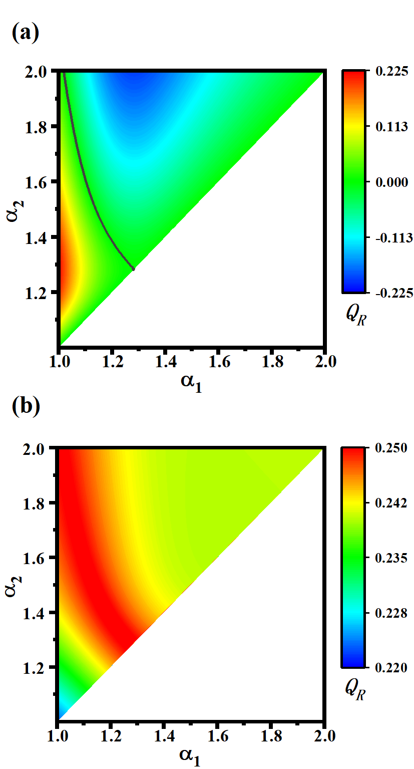
Figure 3: The contour plots of (a) the net heat exchange $Q_{R}$ between the particle and the regenerator and (b) the efficiency $\eta$ varying the fractional parameters $\alpha_{1}$ and $\alpha_{2}$, where $T_{h}=4$, $T_{c}=3$, $m=1$, and $L_{A}=L_{B}=L_{C}=L_{D}=1$. The black line represents the cycle with the perfect regeneration, i.e., $Q_{R}=0$.

In this section, we examine the impact of regulating fractional parameters on the performance of the QSE. The width of the IPW is kept constant throughout the cycle, and the fractional parameter is slowly adjusted from $\alpha_{2}$ ($\alpha_{1})$ to $\alpha_{1}$ ($\alpha_{2})$ during the fractional isothermal process from A to B (C to D), which creates a QSE regulated solely by fractional parameters. To ensure that the cycle proceeds forward, we set $\alpha_{1}<\alpha_{2}$.

By setting $L_{A}=L_{B}=L_{C}=L_{D}=1$ and combining Eqs. (18)-(25), the contour plot of the net heat exchange $Q_{R}$ between the particle and the regenerator varying with $\alpha_{1}$ and $\alpha_{2}$ is obtained, as shown in Fig. 3(a). The plot indicates that $Q_{R}$ is not a monotonic function of $\alpha_{1}$ and $\alpha_{2}$, and the perfect regeneration is able to be achieved by optimizing these parameters [black line in Fig. 3(a)]. The contour plot of the efficiency $\eta$ varying with $\alpha_{1}$ and $\alpha_{2}$ is presented as well [see Fig. 3(b)]. The plot shows that $\eta$ can reach the Carnot efficiency by optimizing $\alpha_{1}$ and $\alpha_{2}$. This is because of the fact that suitable fractional parameters $\alpha_{1}$ and $\alpha_{2}$ lead to perfect regeneration $Q_{R}=0$.

IV.3 THE EFFECTS OF WELL WIDTHS AND FRACTIONAL PARAMETERS

Fig.2 demonstrates that the QSE, which is controlled by the well widths, does not achieve the optimal performance in most regions but can be improved by introducing variational fractional parameters. To further investigate this problem, we modify the isothermal process by adjusting both the widths of the IPW and the fractional parameters simultaneously. As an illustration, we consider the QSE with $L_{A}=1$ and $L_{B}=1.5$, and shows how the engine’s efficiency is enhanced by the fractional parameters.

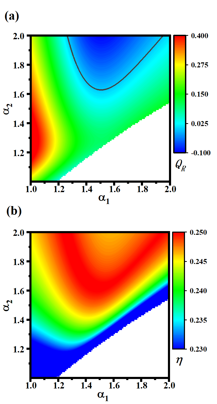
Figure 4: The contour plots of (a) the net heat exchange $Q_{R}$ between the particle and the regenerator and (b) the efficiency $\eta$ varying with the fractional parameters $\alpha_{1}$ and $\alpha_{2}$, where $T_{h}=4$, $T_{c}=3$, $m=1$, $L_{A}=1$, and $L_{B}=1.5$. The black line represents the cycle with the perfect regeneration, i.e., $Q_{R}=0$.

By combining Eqs. (18)-(25), the contour plot of the net heat exchange between the particle and the regenerator $Q_{R}$ of the QSE varying with $\alpha_{1}$ and $\alpha_{2}$ is provided [see Fig. 4(a)]. It can be observed from the figure that $Q_{R}$ is not a monotonic function of $\alpha_{1}$ and $\alpha_{2}$. By optimizing $\alpha_{1}$ and $\alpha_{2}$, the cycle can achieve perfect regeneration with $Q_{R}=0$. At the same time, the contour plot of the efficiency $\eta$ varying with $\alpha_{1}$ and $\alpha_{2}$ is shown in Fig. 4(b). It can be observed from the figure that $\eta$ is also not a monotonic function of $\alpha_{1}$ and $\alpha_{2}$. By optimizing $\alpha_{1}$ and $\alpha_{2}$, $\eta$ can reach the Carnot efficiency. This indicates that the QSE solely regulated by the widths of IPW may lead to a non-ideal regenerative cycle, but the absolute value of the regenerative loss can be reduced and the performance of the QSE can be improved by adjusting the fractional parameters.

$L_{A}$	$L_{B}$	$Q_{r}(\alpha_{1}=\alpha_{2}=2)$	$Q_{r}=0$
			$\alpha_{1}$	$\alpha_{2}$
0.6	0.9	-0.1291	1.245	1.282
	1.0	-0.1315	1.279	1.326
0.8	1.1	-0.01223	1.311	1.409
	1.2	-0.01009	1.382	1.459
1.0	1.3	0.005565	1.439	1.520
	1.4	0.008296	1.502	1.579
1.2	1.5	0.008021	1.517	1.621
	1.6	0.01057	1.565	1.678
1.4	1.7	0.007634	1.607	1.719
	1.8	0.009979	1.660	1.778

Table 1: The values of fractional parameters $\alpha_{1}$ and $\alpha_{2}$ for the perfect regeneration at given values of the widths $L_{A}$ and $L_{B}$.

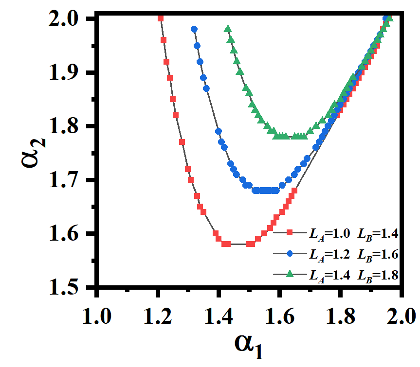
Figure 5: The fractional parameters $\alpha_{1}$ and $\alpha_{2}$ for the perfect regeneration at $L_{A}=1.0,L_{B}=1.4$ (square points), $L_{A}=1.2,L_{B}=1.6$ (circular points), and $L_{A}=1.4,L_{B}=1.8$ (triangular points).

Furthermore, we demonstrate that by adjusting the fractional parameters, the QSE with different well widths can achieve perfect regeneration [see Table 1]. For given values of $L_{A}$ and $L_{B}$, the third column of the table $1$ shows the regenerative loss $Q_{R}$ of the standard QSE ($\alpha_{1}=\alpha_{2}=2$), while the last two columns show the optimal values of $\alpha_{1}$ and $\alpha_{2}$ for the cycle with perfect regeneration. In Fig. 5, we further present the the fractional parameter $\alpha_{1}$ as a function of $\alpha_{2}$ under the condition of perfect regeneration for $L_{A}=1.0,L_{B}=1.4$ (square points), $L_{A}=1.2,L_{B}=1.6$ (circular points), and $L_{A}=1.4,L_{B}=1.8$ (triangular points). Fig.5 shows clearly that for different well widths, the performance of the QSE can be improved through the regulation of fractional parameters, and consequently, the Carnot efficiency can be obtained.

V conclusions

By incorporating the fractional parameter into quantum thermodynamic cycles, we have proposed a new way to regulate thermodynamic cycles based on the fractional quantum mechanics. It is observed that the energy level structure of the system can be changed by adjusting the fractional parameters so that the perfect regeneration and the Carnot efficiency are obtained. This proposal introduces a new approach for designing thermodynamic cycles, when the motion of the particle transits from Brownian motion to Lévy flight. Usually, Brownian motion is driven by white Gaussian noise, whereas the Lévy process can be viewed as a process driven by Lévy noise. Therefore, the introduction of fractional quantum mechanics may provide us with a new route to study thermodynamic processes that are affected by noise or some other heat engines with specific properties. This may also allow us to investigate information theory based on the fractional Schrödinger equation.

APPENDIX A: THE DERIVATION OF THE FRACTIONAL SCHRÖDINGER EQUATION

During an infinitesimal interval $\varepsilon$, the state of the fractional quantum-mechanical system evolves from $\psi(y,t)$ and $\psi(x,t+\varepsilon)$, which is given by

$$\psi(x,t+\varepsilon)=\int_{-\infty}^{\infty}dyK(x,t+\varepsilon\mid y,t)\psi(y,t).$$ (A1)

By using Eq. (1), the continuum limit $\sum_{j=1}^{N}V\left(x_{j}\right)\simeq\int_{t_{a}}^{t_{b}}d\tau V(x(\tau))$, Feynman’s approximation $\int_{t}^{t+\varepsilon}d\tau V(x(\tau))\simeq\varepsilon V\left(\frac{x+y}{2}\right)$, and the kernel

$$K(x,t+\varepsilon\mid y,t)\approx\exp\left[-\frac{i}{\hbar}\varepsilon V\left(\frac{x+y}{2}\right)\right]$$ (A2)

$$\times\lim_{N\rightarrow\infty}\int_{-\infty}^{\infty}dx_{1}\ldots dx_{N-1}\frac{1}{(2\pi\hbar)^{N}}\int_{-\infty}^{\infty}dp_{1}\ldots dp_{N}$$

$$\times\exp\left[\frac{i}{\hbar}\sum_{j=1}^{N}p_{j}\left(x_{j}-x_{j-1}\right)-\frac{i}{\hbar}D_{\alpha}\varepsilon\sum_{j=1}^{N}\left|p_{j}\right|^{\alpha}\right].$$

Note that

$$\sum_{j=1}^{N}p_{j}\left(x_{j}-x_{j-1}\right)=\sum_{j=1}^{N}x_{j}\left(p_{j}-p_{j+1}\right)+p_{N}x_{N}-p_{1}x_{0}$$ (A3)

and the $\delta$ function

$$\delta\left(p_{j}-p_{j+1}\right)=\int dx_{j}\frac{1}{2\pi\hbar}\exp\left[\frac{i}{\hbar}x_{j}\left(p_{j}-p_{j+1}\right)\right],$$ (A4)

Eq. (A2) is simplified as

$$K_{L}(x,t+\varepsilon\mid y,t) =\frac{1}{2\pi\hbar}\int_{-\infty}^{\infty}dp\exp\left[\frac{ip(x-y)}{\hbar}\right.$$ (A5)

$$\left.-\frac{iD_{\alpha}|p|^{\alpha}\varepsilon}{\hbar}-\frac{i}{\hbar}\varepsilon V\left(\frac{x+y}{2},t\right)\right].$$

Substituting Eq. (A5) into Eq. (A1) arrives at

$$\psi(x,t+\varepsilon)= \int_{-\infty}^{\infty}dy\frac{1}{2\pi\hbar}\int_{-\infty}^{\infty}dp$$ (A6)

$$\times\exp\left[\frac{ip(x-y)}{\hbar}\right]\times\exp\left[-\frac{i}{\hbar}D_{\alpha}|p|^{\alpha}\varepsilon\right]$$

$$\times\exp\left[-\frac{i}{\hbar}V\left(\frac{x+y}{2},t\right)\varepsilon\right]\psi(y,t).$$

Expanding the left- and the right-hand sides in power series, taking the first-order approximation and using the definition of Riesz operator in Eq. (4), we have

$$\psi(x,t)+\varepsilon\frac{\partial\psi(x,t)}{\partial t}$$ (A7)

$$=\psi(x,t)+i\frac{D_{\alpha}\varepsilon}{\hbar}(\hbar\nabla)^{\alpha}\psi(x,t)-\frac{i}{\hbar}\varepsilon V(x,t)\psi(x,t),$$

which can be further simplified to obtain Eq. (3).

References

- Herrmann (2011) R. Herrmann, Fractional calculus: an introduction for physicists (World Scientific, 2011).
- Kilbas et al. (1993) A. A. Kilbas, O. I. Marichev, and S. G. Samko, “Fractional integrals and derivatives (theory and applications),” (1993).
- Butzer and Westphal (2000) P. L. Butzer and U. Westphal, in Applications of fractional calculus in physics (World Scientific, 2000) pp. 1–85.
- West (2014) B. J. West, Reviews of modern physics 86, 1169 (2014).
- Guo et al. (2021) L. Guo, Y. Chen, S. Shi, and B. J. West, Fractional Calculus and Applied Analysis 24, 5 (2021).
- Khinchine and Lévy (1936) A. Y. Khinchine and P. Lévy, CR Acad. Sci. Paris 202, 374 (1936).
- Mandelbrot and Mandelbrot (1982) B. B. Mandelbrot and B. B. Mandelbrot, The fractal geometry of nature, Vol. 1 (WH freeman New York, 1982).
- de Jager et al. (2011) M. de Jager, F. J. Weissing, P. M. Herman, B. A. Nolet, and J. van de Koppel, Science 332, 1551 (2011).
- Zaburdaev et al. (2015) V. Zaburdaev, S. Denisov, and J. Klafter, Reviews of Modern Physics 87, 483 (2015).
- Barthelemy et al. (2008) P. Barthelemy, J. Bertolotti, and D. S. Wiersma, Nature 453, 495 (2008).
- Margolin and Barkai (2005) G. Margolin and E. Barkai, Physical review letters 94, 080601 (2005).
- Liu et al. (2016) J. Liu, X. Chen, D. Xu, X. Li, and B. Yang, Wuli Xuebao/Acta Physica Sinica 65 (2016).
- Sagi et al. (2012) Y. Sagi, M. Brook, I. Almog, and N. Davidson, Physical review letters 108, 093002 (2012).
- Laskin (2000a) N. Laskin, Physical Review E 62, 3135 (2000a).
- Laskin (2000b) N. Laskin, Chaos: An Interdisciplinary Journal of Nonlinear Science 10, 780 (2000b).
- Laskin (2000c) N. Laskin, Physics Letters A 268, 298 (2000c).
- Laskin (2002) N. Laskin, Physical Review E 66, 056108 (2002).
- Laskin (2018) N. Laskin, Fractional quantum mechanics (World Scientific, 2018).
- Naber (2004) M. Naber, Journal of mathematical physics 45, 3339 (2004).
- Wang and Xu (2007) S. Wang and M. Xu, Journal of mathematical physics 48, 043502 (2007).
- Dong and Xu (2008) J. Dong and M. Xu, Journal of Mathematical Analysis and Applications 344, 1005 (2008).
- Felmer et al. (2012) P. Felmer, A. Quaas, and J. Tan, Proceedings of the Royal Society of Edinburgh Section A: Mathematics 142, 1237 (2012).
- Secchi (2013) S. Secchi, Journal of Mathematical Physics 54, 031501 (2013).
- Fall et al. (2015) M. M. Fall, F. Mahmoudi, and E. Valdinoci, Nonlinearity 28, 1937 (2015).
- Wei (2015) Y. Wei, Int. J. Theor. Math. Phys. 5, 87 (2015).
- Longhi (2015) S. Longhi, Optics letters 40, 1117 (2015).
- Laskin (2017) N. Laskin, Chaos, Solitons & Fractals 102, 16 (2017).
- Liu et al. (2023) S. Liu, Y. Zhang, B. A. Malomed, and E. Karimi, Nature Communications 14, 222 (2023).
- Mainardi (1997) F. Mainardi, Fractional calculus: some basic problems in continuum and statistical mechanics (Springer, 1997).
- Tudor and Viens (2007) C. A. Tudor and F. G. Viens, (2007).
- Wang et al. (2014) C.-Y. Wang, X.-M. Zong, H. Zhang, and M. Yi, Physical Review E 90, 022126 (2014).
- Meilanov and Magomedov (2014) R. Meilanov and R. Magomedov, Journal of Engineering physics and thermophysics 87, 1521 (2014).
- Bagci (2016) G. B. Bagci, Physics Letters A 380, 2615 (2016).
- Lopes and Machado (2020) A. M. Lopes and J. A. T. Machado, Entropy 22, 1374 (2020).
- Tarasov (2006) V. E. Tarasov, Chaos: An Interdisciplinary Journal of Nonlinear Science 16, 033108 (2006).
- Sisman and Fransson (2021) A. Sisman and J. Fransson, Physical Review E 104, 054110 (2021).
- Khadem et al. (2022) S. M. J. Khadem, R. Klages, and S. H. Klapp, Physical Review Research 4, 043186 (2022).
- Korichi et al. (2022) N. Korichi, A. Boumali, and H. Hassanabadi, Physica A: Statistical Mechanics and its Applications 587, 126508 (2022).
- Jalalzadeh et al. (2021) S. Jalalzadeh, F. R. da Silva, and P. Moniz, The European Physical Journal C 81, 632 (2021).
- Scovil and Schulz-DuBois (1959) H. E. Scovil and E. O. Schulz-DuBois, Physical Review Letters 2, 262 (1959).
- Geusic et al. (1967) J. Geusic, E. Schulz-DuBios, and H. Scovil, Physical Review 156, 343 (1967).
- Quan et al. (2005) H. Quan, P. Zhang, and C. Sun, Physical Review E 72, 056110 (2005).
- Kieu (2006) T. D. Kieu, The European Physical Journal D-Atomic, Molecular, Optical and Plasma Physics 39, 115 (2006).
- Quan et al. (2007) H.-T. Quan, Y.-x. Liu, C.-P. Sun, and F. Nori, Physical Review E 76, 031105 (2007).
- Wu et al. (1998) F. Wu, L. Chen, F. Sun, C. Wu, and Y. Zhu, Energy conversion and management 39, 733 (1998).
- Huang et al. (2014) X.-L. Huang, X.-Y. Niu, X.-M. Xiu, and X.-X. Yi, The European Physical Journal D 68, 1 (2014).
- Su et al. (2018) S. Su, J. Chen, Y. Ma, J. Chen, and C. Sun, Chinese Physics B 27, 060502 (2018).
- Chen (1997) J. Chen, International journal of ambient energy 18, 107 (1997).
- Chen et al. (1998) J. Chen, Z. Yan, L. Chen, and B. Andresen, International journal of energy research 22, 805 (1998).