Tractable Probabilistic Graph Representation
Learning with Graph-Induced Sum-Product Networks

Abstract

We introduce Graph-Induced Sum-Product Networks (GSPNs), a new probabilistic framework for graph representation learning that can tractably answer probabilistic queries. Inspired by the computational trees induced by vertices in the context of message-passing neural networks, we build hierarchies of sum-product networks (SPNs) where the parameters of a parent SPN are learnable transformations of the a-posterior mixing probabilities of its children’s sum units. Due to weight sharing and the tree-shaped computation graphs of GSPNs, we obtain the efficiency and efficacy of deep graph networks with the additional advantages of a purely probabilistic model. We show the model’s competitiveness on scarce supervision scenarios, handling missing data, and graph classification in comparison to popular neural models. We complement the experiments with qualitative analyses on hyper-parameters and the model’s ability to answer probabilistic queries.

1 Introduction

As the machine learning field advances towards highly effective models for language, vision, and applications in the sciences and engineering, many practical challenges stand in the way of widespread adoption. Overconfident predictions are hard to trust, and most current models are not able to provide uncertainty estimates of predictions and to support counterfactual “what if” questions [37, 26, 32]. Capturing such functionality requires the ability to efficiently answer probabilistic queries, e.g., computing the likelihood or marginals and, therefore, learning tractable distributions [10]. Such capabilities would not only increase the trustworthiness of learning systems but also allow us to naturally cope with missing information in the input through marginalization, avoiding the use of ad-hoc imputation methods; this is another desideratum in applications where data (labels and attributes) is often incomplete [12, 69]. In numerous application domains, obtaining labeled data is expensive, and while large unlabeled data sets might be available, this does not imply the availability of ground-truth labels. This is the case, for instance, in the medical domains [51] where the labeling process must comply with privacy regulations and in the chemical domain where one gathers target labels via costly simulations or in-vitro experiments [21].

In this work, we are interested in data represented as a graph. Graphs are a useful representational paradigm in a large number of scientific disciplines such as chemistry and biology. The field of Graph Representation Learning (GRL) is concerned with the design of learning approaches that directly model the structural dependencies inherent in graphs [6, 20, 68, 59, 4]. The majority of GRL methods implicitly induce a computational directed acyclic graph (DAG) for each vertex in the input graph, alternating learnable message passing and aggregation steps [18, 4]. Most of these approaches exclusively rely on neural network components in these computation graphs, but cannot answer probabilistic queries nor exploit the vast amount of unlabeled data.

Motivated by these considerations, we propose a class of hierarchical probabilistic models for graphs called GSPNs, which can tractably answer a class of probabilistic queries of interest and whose computation graphs are also (DAGs). While GSPNs are computationally as efficient as Deep Graph Networks (DGNs), they consist of a hierarchy of interconnected sum-product networks. GSPNs can easily handle missing data in graphs and answer counterfactual probabilistic queries that indicate a change in likelihood under specific changes of vertex attribute values. The learned probabilistic graph representations are also competitive with state-of-the-art deep graph networks in the scarce supervision and graph classification settings.

2 Related Work

Unsupervised learning for graphs is under-explored relative to the large body of work on supervised graph representation learning [44, 33, 35, 29, 53, 60, 64]. Contrary to self-supervised pre-training [25] which investigates ad-hoc learning objectives, unsupervised learning encompasses a broader class of models that extract patterns from unlabeled data. Most unsupervised approaches for graphs currently rely on i) auto-encoders, such as the Graph Auto-Encoder (GAE) [28] and ii) contrastive learning, with Deep Graph Infomax (DGI) [54] adapting ideas from computer vision and information theory to graph-structured data. While the former learns to reconstruct edges, the latter compares the input graph against its corrupted version and learns to produce different representations.

Existing probabilistic approaches to unsupervised deep learning on graphs often deal with clustering and Probability Density Estimation (PDE) problems; a classic example is the Gaussian Mixture Model (GMM) [5] capturing multi-modal distributions of Euclidean data. The field of Statistical Relational Learning (SRL) considers domains where we require both uncertainty and complex relations; ideas from SRL have recently led to new variational frameworks for (un-)supervised vertex classification [41]. The Contextual Graph Markov Model (CGMM) [3] and its variants [1, 7] are unsupervised DGNs trained incrementally, i.e., layer after layer, which have been successfully applied to graph classification tasks. Their incremental training grants closed-form learning equations at each layer, but it comes at the price of no global cooperation towards the optimization of the learning objective, i.e., the likelihood of the data; this makes it impractical for answering missing data queries.

So far, the literature on missing data in graphs, i.e., using the graph structure to handle missing attribute values, has not received as much attention as other problems. Recent work focuses on mitigating “missingness” in vertex classification tasks [42] or representing missing information as a learned vector of parameters [31], but the quality of the learned data distribution has not been discussed so far (to the best of our knowledge). There are some attempts at imputing vertex attributes through a GMM [50], but such a process does not take into account the available graph structure. Similarly, other proposals [8] deal with the imputation of vertices having either all or none of their attributes missing, a rather unrealistic assumption for most cases. In this work, we propose an approach that captures the data distribution under missing vertex attribute values and requires no imputation.

3 Background

We define a graph $g$ as a triple $(\mathcal{V},\mathcal{E},\mathcal{\bm{X}})$, where $\mathcal{V}=\{1,\dots,N\}$ denotes the set of $N$ vertices, $\mathcal{E}$ is the set of directed edges $(u,v)$ connecting vertex $u$ to $v$, and $\mathcal{\bm{X}}=\{\bm{x}_{u}\in\mathbb{R}^{d},d\in\mathbb{N},\forall u\in\mathcal{V}\}$ represents the the set of vertex attributes. In this work, we do not consider edge attributes. The neighborhood of a vertex $v$ is the set $\mathcal{N}_{v}=\{u\in\mathcal{V}\mid(u,v)\in\mathcal{E}\}$ of incoming edges. Also, access to the $i$-th component of a vector $\bm{x}$ shall be denoted by $\bm{x}(i)$ and that of a function $f$’s output as $f(\cdot)_{i}$.

Graph Representation Learning

Learning on graph-structured data typically means that one seeks a mapping from an input graph to vertex embeddings [15], and such a mapping should be able to deal with graphs of varying topology. In general, a vertex $v$’s representation is a vector $\bm{h}_{v}\in\mathbb{R}^{C},C\in\mathbb{N}$ encoding information about the vertex and its neighboring context, so that predictions about $v$ can be then made by feeding $\bm{h}_{v}$ into a classical ML predictor. In graph classification or regression, instead, these vertex representations have to be globally aggregated using permutation invariant operators such as the sum or mean, resulting in a single representation $\bm{h}_{g}\in\mathbb{R}^{C}$ of the entire graph that is used by the subsequent predictor. At the time of this writing, message-passing neural networks (MPNN) [18] are the most popular class of methods to compute vertex representations. These methods adopt a local and iterative processing of information, in which each vertex repeatedly receives messages from its incoming connections, aggregates these messages, and sends new messages along the outgoing edges. Researchers have developed several variants of this scheme, starting from the two pioneering methods: the recurrent Graph Neural Network (GNN) of Scarselli et al. [44] and the feedforward Neural Network for Graphs (NN4G) of Micheli [33].

Tractable Probabilistic Models

Probabilistic Circuits (PCs) are probabilistic models that can tractably, i.e., with polynomial complexity in the size of the circuit, answer a large class of probabilistic queries [10] and can be trained via backpropagation. A PC is usually composed of distribution units, representing distributions over one or more random variables, product units computing the fully factorized joint distribution of its children, and the sum units encoding mixtures of the children’s distributions. Sum-Product Networks (SPNs) [40, 16, 52, 46] are a special class of PCs that support tractable computation of joint, marginal, and conditional distributions, which we will exploit to easily handle missing data. Informally, a (locally normalized) SPN is a probabilistic model defined via a rooted computational DAG, whose parameters of every sum unit add up to 1 [55]. Furthermore, the scope of an SPN is the set of its distribution units, and valid SPNs represent proper distributions. For instance, a GMM and a Naïve Bayes model (NB) [58] can both be written as SPNs with a single sum unit. While the class of PCs is equivalent to that of deep mixture models [38], PCs are not probabilistic graphical models (PGMs) [30]: the former specify an operational semantics describing how to compute probabilities, whereas the representational semantics of the latter specifies the conditional independence of the variables involved. Crucially, for valid SPNs and an arbitrary sum unit $j$ with $C$ children, it is always possible to tractably compute its posterior distribution, parametrized by the vector $\bm{h}_{j}\in\mathbb{R}^{C}$ [38]. Here, we are voluntarily abusing the notation because in the following we will consider posterior distributions of sum nodes as our latent representations. Due to space constraints, we provide a more detailed introduction to PCs in Section A.1.

4 GSPN: Learning Tractable Probabilistic Graph Representations

Figure 1: Inference on the graphical model on the left is typically unfeasible due to the mutual dependencies induced by cycles. Therefore, we approximate the learning problem using probabilistic computational trees of height $L$ modeled by a hierarchy of tractable SPNs (right).

When one considers a cyclic graphical model such as the one on the left-hand-side of Figure 1, probabilistic inference is computationally infeasible unless we make specific assumptions to break the mutual dependencies between the random variables (r.v.) $Q$, depicted as white circles. To address this issue, we model tractable probability distributions over attributed graphs as products of conditional distributions, one for each vertex in the graph. The scope of these distributions consists of the $L$-hop neighborhoods induced by a traversal of the graph rooted at said vertex. Akin to what done for DGNs, the parameters of the conditional distributions are shared across vertices.

We propose a class of models whose ability to tractably answer queries stems from a hierarchical composition of sum-product networks (SPNs). To describe the construction of this hierarchical model we consider, for each vertex $v$ in the input graph, a tree rooted at $v$ of height $L$, where $L$ is a hyper-parameter. To distinguish between graphs and trees, we use the terms vertices for the graphs and nodes for the trees. Moreover, because graph cycles induce repetitions in the computational trees, we have to use a new indexing system: given a tree, we denote by $m(\cdot)$ a mapping from its node index $n$ to a vertex $u$ in the input graph.
We now formally define the tree of height $L$ rooted at vertex $v$ as follows. First, we have one root node $n$ with $m(n)=v$ and $n$ having height $L$. Second, for a node $n$ in the tree at height $1\leq\ell\leq L$, we have that a node $n^{\prime}$ is a child of $n$ with height $\ell-1$ if and only if vertex $v^{\prime}=m(n^{\prime})$ is in the $1$-hop neighborhood of vertex $u=m(n)$. Similarly, when vertex $u$ does not have $1$-hop neighbors and $\ell>0$, the node $n^{\prime},u=m(n^{\prime})$ is the single child of $n,u=m(n)$ (i.e., we add self-loops to handle isolated vertices). Finally, every node $n$ at height $\ell=0$ is a leaf node and has no children. Figure 1 (center) depicts examples of trees induced by the nodes of the graph on the left.

We use the structure of each graph-induced tree as a blueprint to create a hierarchy of normalized SPNs, where all SPNs have the same internal structure. Every node of a tree is associated with a valid SPN whose scope consists of the random variables $A_{1},\dots,A_{d}$ modeling the vertex attributes, meaning the distribution units of said SPN are tractable distributions for the variable $\bm{X}=(A_{1},...,A_{d})$. To distinguish between the various distributions for the r.v. $\bm{X}$ modeled by the SPNs at different nodes, we introduce for every node $n$ and every height $\ell$, the r.v. $\bm{X}_{n}^{\ell}$ with realization $\bm{x}_{m(n)}$. The parameters of the tractable distribution units int the SPN of node $n$ at height $\ell$ are denoted by $\bm{\omega}_{n}^{\ell}$, which are shared across the nodes at the same height. Moreover, the mixture probabilities of the $S$ sum nodes in the SPN of node $n$ at height $\ell$ are denoted by $\bm{\pi}_{n,j}^{\ell}$, $1\leq j\leq S$.

To obtain a hierarchical model, that is, to connect the SPNs according to the tree structure, we proceed as follows. For every SPN of a non-leaf node $n$, the parameters $\bm{\pi}_{n,j}^{\ell}$ of sum unit $j$ are learnable transformations of the posterior probabilities of the sum units $j$ in the children SPNs. More formally, let $n_{1},\dots,n_{T}$ be the children of a node $n$ and let $\bm{h}_{n_{i},j}^{\ell-1}$ be the vector of posterior probabilities of sum unit $j$ for the SPN of node $n_{i}$. Then, $\bm{\pi}_{n,j}^{\ell}=f_{\bm{\theta}_{j}^{\ell}}(\bm{h}_{n_{1},j}^{\ell-1},\dots,\bm{h}_{n_{T},j}^{\ell-1})$ with learnable parameters $\bm{\theta}_{j}^{\ell}$ shared across level $\ell$. The choice of $f$ does not depend on the specific SPN template, but it has to be permutation invariant because it acts as the neighborhood aggregation function of message-passing methods. The parameters of the sum units of leaf nodes, $\bm{\pi}_{j}^{0}$, are learnable and shared. Figure 1 (right) illustrates the hierarchical composition of SPNs according to a tree in Figure 1 (center). Moreover, Figure 2 illustrates how the prior distribution of the SPNs at height $1$ is parametrized by a learnable transformation of posterior mixture probabilities of its children SPNs, similar to what is done by Vergari et al. [56] with fixed Dirichlet priors.

A graph $g$ in the training data specifies (partial) evidence $\bm{x}_{v}$ for every one of its vertices $v$. The hierarchical SPN generated for $v$ now defines a tractable probability distribution for the root node conditioned on the (partial) evidence for its intermediate nodes, which we can compute by evaluating the hierarchical SPNs tree in a bottom-up fashion. For some vertex $v$ in the graph, let $n_{2},\dots,n_{T_{v}}$ be the nodes of the graph-induced tree rooted at $v$, without the root node $n_{1}$ itself. Given partial evidence for the tree $\bm{x}_{m(n_{i})}$, $1\leq i\leq T_{v}$, the objective is to maximize the pseudo log-likelihood of the attribute values at root node $v$ given the attribute values at all other nodes in its tree:

$$\log\prod_{v\in\mathcal{V}}P_{\bm{\Theta}}(\bm{x}_{m_{v}(n_{1})}\mid\bm{x}_{m_{v}(n_{2})},\dots,\bm{x}_{m_{v}(n_{T_{v}})}),$$ (1)

where $P_{\bm{\Theta}}$ is the conditional probability defined by the hierarchical SPN for $v$ with parameters $\bm{\Theta}$ and we have added a sub-index to $m_{v}(\cdot)$ to make the mapping function tree-specific.

4.1 Naive Bayes GSPNs

An instance of the proposed framework uses Naïve Bayes models as base SPNs, shown in Figure 2 in both their graphical and SPN representations for two continuous vertex attributes. There is a single categorical latent r.v. $Q$ with $C$ possible states. Let us denote this latent r.v. for node $n$ at height $\ell$ in the tree as $Q_{n}^{\ell}$ and its prior distribution as $P_{\bm{\pi}_{n}^{\ell}}(Q_{n}^{\ell})$. Due to the assumption that all r.v.s $\bm{X}_{n}^{\ell}$ have tractable distributions, we have, for all $\ell,n$ and $i$, that the conditional distribution $P_{\bm{\omega}_{n}^{\ell}}(\bm{X}_{n}^{\ell}\mid Q_{n}^{\ell}=i)$ is tractable. Moreover, for each child node $n$ at height $\ell$ we have that

$$\bm{h}_{n}^{\ell}(i)=P(Q^{\ell}_{n}=i\mid\bm{X}^{\ell}_{n}=\bm{x}_{m(n)}).$$ (2)

For each leaf $n$ of a tree, the posterior probabilities for the SPNs sum unit are given by

$$\bm{h}^{0}_{n}(i) =P(Q^{0}_{n}=i\mid\bm{X}^{0}_{n}=\bm{x}_{m(n)})=\frac{P_{\bm{\omega}_{n}^{0}}(\bm{x}_{m(n)}\mid Q^{0}_{n}=i)P_{\bm{\pi}_{n}^{0}}(Q^{0}_{n}=i)}{\sum_{i^{\prime}}^{C}P_{\bm{\omega}_{n}^{0}}(\bm{x}_{m(n)}\mid Q^{0}_{n}=i^{\prime})P_{\bm{\pi}_{n}^{0}}(Q^{0}_{n}=i^{\prime})},$$ (3)

where $\bm{\pi}_{n}^{0}$ is learned and shared across leaf nodes. For $\ell\geq 1$, the latent priors $P_{\bm{\pi}_{n}^{\ell}}(Q_{n}^{\ell})$ are parametrized by the output of a learnable transformation of the posterior probabilities of the sum units of the child SPNs. More formally, for node $n^{\prime}$ at height $\ell+1,\ell\geq 0$, and with children $ch(n^{\prime})$ we compute the prior probabilities $\bm{\pi}_{n^{\prime}}^{\ell+1}$ as

$$\bm{\pi}_{n^{\prime}}^{\ell+1}=f_{\bm{\theta}^{\ell+1}}(\bm{h}^{\ell}_{1},...,\bm{h}^{\ell}_{|ch_{n^{\prime}}|}), \bm{h}^{\ell}_{n}(i)=\frac{P_{\bm{\omega}_{n}^{\ell}}(\bm{x}_{m(n)}\mid Q^{\ell}_{n}=i)P_{\bm{\pi}_{n}^{\ell}}(Q^{\ell}_{n}=i)}{\sum_{i^{\prime}}^{C}P_{\bm{\omega}_{n}^{\ell}}(\bm{x}_{m(n)}\mid Q^{\ell}_{n}=i^{\prime})P_{\bm{\pi}_{n}^{\ell}}(Q^{\ell}_{n}=i^{\prime})},$$ (4)

noting that the posterior $\bm{h}^{\ell}_{n}$ is tractable as the quantities of interest are obtained with a single backward pass in the SPN [38]. Figure 2 visualizes how $f_{\bm{\theta}^{1}}$ acts on the prior probabilities in the example of Figure 1. In the experiments, we define $f_{\bm{\theta}^{\ell+1}}(\bm{h}^{\ell}_{1},...,\bm{h}^{\ell}_{|ch_{n^{\prime}}|})=\frac{1}{|ch_{n^{\prime}}|}\sum_{n\in ch_{n^{\prime}}}\bm{\theta}^{\ell+1}\bm{h}^{\ell}_{n}$ for a learnable transition matrix $\bm{\theta}^{\ell+1}\in\mathbb{R}^{C\times C}$ that specifies how much a child’s (soft) state $k$ contributes to the weight of state $i$ in the new prior distribution $P_{\bm{\pi}_{n^{\prime}}^{\ell+1}}(Q^{\ell+1}_{n^{\prime}}=i)$. Each row $k$ of $\bm{\theta}^{\ell+1}$ must specify a valid probability over $C$ possible states, enforced through normalization techniques. The function is motivated by the observation that it corresponds to applying the “Switching Parent” decomposition to the conditional mixture model defined in [3] (deferred to Section A.2 due to space constraints). Likewise, we show in Section A.3 that Equation 4 produces a valid parametrization for the new prior distribution.

Figure 2: (Left) We expand the example of Figure 1 to illustrate how the prior distribution of the top SPN (here the Naïve Bayes on the right) is parametrized by a learnable transformation of the children’s SPNs posterior mixture probabilities. (Right) A Gaussian Naïve Bayes graphical model with r.v. $\bm{X}=(A_{1},A_{2})$ and its equivalent SPN with scope $\{A_{1},A_{2}\}$.

This iterative process can be implemented in the exact same way message passing is implemented in neural networks, because the computation for trees of height $\ell$ can be reused in trees of height $\ell+1$. Furthermore, our choice of $f_{\bm{\theta}^{\ell}}$ leads to a fully probabilistic formulation and interpretation of end-to-end message passing on graphs. Motivated by studies on the application of gradient ascent for mixture models and SPNs [61, 47, 38, 17], we maximize Equation 1 with backpropagation. We can execute all probabilistic operations on GPU to speed up the computation, whose overall complexity is linear in the number of edges as in most DGNs. For the interested reader, Section A.4 describes how GSPN can be applied to more general SPNs with multiple sum units and provides the pseudocode for the general inference phase.

4.2 Modeling Missing Data

With GSPNs we can deal with partial evidence of the graph, or missing attribute values, in a sound probabilistic manner. This is a distinctive characteristic of our proposal compared to previous probabilistic methods for vectors, as GSPNs can tractably answer probabilistic queries on graphs by also leveraging their structural information. We take inspiration from the EM algorithm for missing data [27]: in particular, let us consider a multivariate r.v. of a root node $\bm{X}$ (dropping other indices for ease of notation) as a tuple of observed and missing sets of variables, i.e., $\bm{X}=(\bm{X}^{obs},\bm{X}^{mis})$. When computing the posterior probabilities of sum nodes $\bm{h}$, we have to modify Equations 3 and 4 to only account for $\bm{X}^{obs}$; in SPNs, this equals to setting the distribution units of the missing attributes to 1 when computing marginals, causing the missing variables to be marginalized out. This can be computed efficiently due to the decomposability property of the SPNs used in this work [11]. Additionally, if we wanted to impute missing attributes for a vertex $v$, we could apply the conditional mean imputation strategy [69] to the corresponding root r.v. of the tree $\bm{X}_{1}^{L}=(\bm{X}_{1}^{obs},\bm{X}_{1}^{mis})$ for $v$, which, for the specific case of NB, corresponds to $\bm{x}_{v}^{mis}=\sum_{i}^{C}\mathbb{E}\big{[}\bm{X}_{1}^{mis}\mid Q^{L}_{1}=i\big{]}*\bm{h}^{L}_{1}(i)$. Hence, to impute the missing attributes of $\bm{x}_{v}$, we sum the (average) predictions of each mixture in the top SPN, where the mixing weights are given by the posterior distribution. The reason is that the posterior distribution carries information about our beliefs after observing $\bm{X}^{obs}_{v}$.

4.3 A Global Readout for Supervised Learning

Using similar arguments as before, we can build a probabilistic and supervised extension of GSPN for graph regression and classification tasks. It is sufficient to consider a new tree where the root node $r$ is associated with the target r.v. $Y$ and the children are all possible trees of different heights rooted at the $N$ vertices of graph $g$. Then, we build an SPN for $r$ whose sum unit $j$ is parametrized by a learnable tansformation $\bm{\pi}_{r,j}=f_{\bm{\vartheta}_{j}}(\cdot).$ This function receives the set $\bm{h}_{\mathcal{V},j}$ of outputs $\bm{h}^{\ell}_{u,j}$ associated with the top SPN related to the graph-induced tree of height $\ell$ rooted at $u$, for $0\leq\ell\leq L$. In other words, this is equivalent to consider all vertex representations computed by a DGN at different layers.
For NB models with one sum unit, given (partial) evidence $\bm{x}_{1},\dots,\bm{x}_{N}$ for all nodes, we write

$$P_{\bm{}}(\bm{y}\mid\bm{x}_{1},\dots,\bm{x}_{N})=\sum_{i=1}^{C_{g}}P_{\bm{\omega}}(\bm{y}\mid Q=i)P_{\bm{\pi}_{r}}(Q=i),\ \ \bm{\pi}_{r}\overset{\mathrm{def}}{=}f_{\bm{\vartheta}}(\bm{h}_{\mathcal{V}})=\Omega\big{(}\sum_{u\in\mathcal{V}}\sum_{\ell=1}^{L}\bm{\vartheta}^{\ell}\bm{h}^{\ell}_{u}\big{)},$$ (5)

where $\bm{\omega}$ and $\bm{\pi}_{r}$ are the parameters of the NB and $Q$ is a latent categorical variable with $C_{g}$ states. Computing $\bm{\pi}_{r}$ essentially corresponds to a global pooling operation, where $\bm{\vartheta}^{\ell}\in\mathbb{R}^{C_{g}\times C}$ is another transition matrix and $\Omega$ can be $\frac{1}{LN}$ (resp. the softmax function) for mean (resp. sum) global pooling. We treat the choice of $\Omega(\cdot)$ as a hyper-parameter, and the resulting model is called GSPN_S.

4.4 Probabilistic Shortcut Connections

We propose probabilistic shortcut connections as a mechanism to set the emission parameters at the root $\bm{\omega}^{L}$ as a convex combination of the emission parameters at height $\{\bm{\omega}^{0},\dots,\bm{\omega}^{L-1}\}$. For instance, for a continuous r.v. $\tilde{\bm{X}}_{n}^{L}$ of the root node $n$, a modeling choice would be to take the mean of the $L-1$ Gaussians implementing the emission distributions, leveraging known statistical properties to obtain

$$P_{\bm{\omega}^{L}}(\tilde{\bm{X}}_{n}^{L}\mid Q^{L}_{n}=i)\overset{\mathrm{def}}{=}\mathcal{N}\left(\cdot\ ;\sum_{\ell=1}^{L-1}\frac{\mu^{\ell}_{i}}{L-1},\sum_{\ell=1}^{L-1}\frac{(\sigma^{\ell}_{i})^{2}}{(L-1)^{2}}\right),\ \ \bm{\omega}^{\ell}=(\mu^{\ell}_{1},\sigma^{\ell}_{1},\dots,\mu^{\ell}_{C},\sigma^{\ell}_{C}).$$ (6)

Instead, when the r.v. is categorical, we consider a newly parametrized Categorical distribution:

$$P_{\bm{\omega}^{L}}(\tilde{\bm{X}}_{n}^{L}\mid Q^{L}_{n}=i)\overset{\mathrm{def}}{=}Cat\left(\cdot\ ;\sum_{\ell=1}^{L-1}\frac{\bm{\omega}^{\ell}_{i}}{L-1}\right),\bm{\omega}^{\ell}_{i}\in C\text{-1-probability simplex}\ \ \forall i\in[1,C].$$ (7)

Akin to residual connections in neural networks [49, 22], these shortcut connections mitigate the vanishing gradient and the degradation (accuracy saturation) problem, that is, the problem of more layers leading to higher training error. In the experiments, we treat the choice of using residual connections as a hyper-parameter and postpone more complex design choices, such as weighted residual connections, to future work.

4.5 Limitations

Due to the problem of modeling an inherently intractable probability distribution defined over a cyclic graph, GSPNs have to rely on a composition of locally valid SPNs to tractably answer probabilistic queries. For this reason, GSPNs are akin to hierarchical probabilistic models where the posterior distribution of a variable is used to determine prior probabilities of another distribution. Also, one needs to specify a tractable parametric family of distribution for each attribute; as with other probabilistic models, numerical over- and underflow errors are more likely compared to purely neural network-based approaches, especially as the number of attributes increases. From the point of view of expressiveness in distinguishing non-isomorphic graphs, past results tell us that more powerful aggregations would be possible if we explored a different neighborhood aggregation scheme [60]. In this work, we keep the neighborhood aggregation functions $f_{\bm{\theta}}$ as simple as possible to get a fully probabilistic model with valid and more interpretable probabilities. Finally, GSPN is currently unable to model edge types, which would enable us to capture a broader class of graphs.

5 Experiments

We consider three different classes of experiments as described in the next sections. Code and data to reproduce the results will be released in the future.

Scarce Supervision

Akin to Erhan et al. [13] for non-structured data, we show that unsupervised learning can be very helpful in the scarce supervision scenario by exploiting large amounts of unlabeled data. We select seven chemical graph regression problems, namely benzene, ethanol, naphthalene, salicylic acid, toluene, malonaldehyde and uracil [9], using categorical atom types as attributes, and ogbg-molpcba, an imbalanced multi-label classification task [24]. Given the size of the datasets, we perform a hold-out risk assessment procedure (90% training, 10% test) with internal hold-out model selection (using 10% of the training data for validation) and a final re-training of the selected configuration. In the case of ogbg-molpcba, we use the publicly available data splits. Mean Average Error (MAE) is the main evaluation metric for all chemical tasks except for ogbg-molpcba (Average Precision – AP – averaged across tasks). We first train a GSPN_U on the whole training set to produce unsupervised vertex embeddings, and then we fit a DeepSets (DS) [66] classifier on just $0.1\%$ of the supervised samples using the learned embeddings. We do not include GSPN_S in the analysis because, as expected, the scarce supervision led to training instability during preliminary experiments.
We compare against two effective and well-known unsupervised models, the Graph Auto-Encoder (GAE) and Deep Graph Infomax (DGI). These models have different unsupervised objectives: the former is trained to reconstruct the adjacency matrix whereas the second is trained with a contrastive learning criterion. Comparing GSPN_U, which maximizes the vertices’ pseudo log-likelihood, against these baselines will shed light on the practical usefulness of our learning strategy. In addition, we consider the GIN model [60] trained exclusively on the labeled training samples as it is one of the most popular DGNs in the literature. We summarize the space of hyper-parameter configurations for all models in Table 4.

Modeling the Data Distribution under Partial Evidence

We analyze GSPN’s ability at modeling the data distribution under missing values on synthetic and real-world datasets. Synthetic datasets allow us to study the behavior of models under more precise conditions [36]. Each such dataset has $10,000$ graphs sampled from an Erdös-Rényi Stochastic Block Model [23] with an attribute generation mechanism that satisfies the conditions of Section 4.2. We defer the details of the generative process to Section A.5. We test 3 different versions of the dataset, namely Syn₀, Syn_0.5 and Syn₁ depending on how much influence the neighborhood has (0 = no effect and 1 = max effect) on the generation of vertex attributes. We use the same evaluation and data split strategies of the previous experiment. As for the real-world datasets, we re-use the same datasets as before using their 6 available continuous attributes (except for ogbg-molpcba that has only categorical values).
For each vertex, we randomly mask a proportion of the attributes given by a sample from a Gamma distribution with concentration $1.5$ and rate $1/2$). We do so to simulate a plausible scenario in which many vertices have few attributes missing and few vertices have many missing attributes. The evaluation metric is the negative pseudo log-likelihood of Equation 1 (NLL) to understand how well GSPNs can exploit the structure to model the (partial) evidence.
The first baseline is a simple Gaussian distribution, which computes its sufficient statistics (mean and standard deviation) from the training set and then computes the NLL on the dataset. The second baseline is a structure-agnostic Gaussian Mixture Model (GMM), which does not rely on the structure when performing imputation but can model arbitrarily complex distributions; we recall that our model behaves like a GMM when the number of layers is set to 1. The set of hyper-parameters configurations tried for each baseline is reported in Table 5.

Graph Classification

Among the graph classification tasks of Errica et al. [14], we restrict our evaluation to NCI1 [57], REDDIT-BINARY, REDDIT-MULTI-5K, and COLLAB [63] datasets, for which leveraging the structure seems to help improving the performances. The empirical setup and data splits are the same as Errica et al. [14], Castellana et al. [7], from which we report previous results. The baselines we compare against are a structure-agnostic baseline (Baseline), DGCNN [67], DiffPool [65], ECC [48], GIN [60], GraphSAGE [19], CGMM, E-CGMM [1], and iCGMM [7]. CGMM can be seen as an incrementally trained version of GSPN that cannot use probabilistic shortcut connections. Table 6 shows the set of hyper-parameters tried for GSPN, and Table 10 shows that the time to compute a forward and backward pass of GSPN is comparable to GIN.

6 Results

We present quantitative and qualitative results following the structure of Section 5. For all experiments we used a server with $32$ cores, $128$ GBs of RAM, and $8$ GPUs with $32$ GBs of memory.

Scarce Supervision

Table 1: Mean and std results on scarce supervision tasks averaged over 10 runs, with $0.1\%$. The best and second-best average results are bold and underlined, respectively.

Model	GIN	GAE+DS	DGI+DS	GSPNU+DS
Eval. Process	Sup.	Unsup.$\rightarrow$ Sup.	Unsup.$\rightarrow$ Sup.	Unsup.$\rightarrow$ Sup.
benzene	41.4 $\pm$ 45.6	$\mathbf{2.00}$ $\pm$ 0.1	6.22 $\pm$ 1.2	2.24 $\pm$ 0.5
ethanol	4.00 $\pm$ 1.0	7.79 $\pm$ 7.8	5.35 $\pm$ 3.5	$\mathbf{3.36}$ $\pm$ 0.0
malonaldehyde	8.00 $\pm$ 5.3	5.49 $\pm$ 1.3	$\mathbf{4.31}$ $\pm$ 1.8	$\mathbf{4.31}$ $\pm$ 1.4
naphthalene	34.9 $\pm$ 19.4	4.45 $\pm$ 0.3	6.34 $\pm$ 2.3	$\mathbf{4.44}$ $\pm$ 0.1
salicylic acid	36.7 $\pm$ 13.4	233.3 $\pm$ 27.1	17.0 $\pm$ 7.3	$\mathbf{4.90}$ $\pm$ 0.5
toluene	29.6 $\pm$ 18.0	$\mathbf{4.83}$ $\pm$ 0.3	9.18 $\pm$ 0.3	4.87 $\pm$ 1.4
uracil	19.7 $\pm$ 14.1	387.7 $\pm$ 13.7	409.7 $\pm$ 1.5	$\mathbf{3.93}$ $\pm$ 0.0
ogbg-molpcba ($\uparrow$)	$\mathbf{4.12}$ $\pm$ 0.2	3.36 $\pm$ 0.3	3.00 $\pm 0.5$	4.00 $\pm 0.5$

In Table 1, we report the performance of GSPN_U combined with DeepSets (DS) in the scarce supervision scenario. We make the following observations. First, a fully supervised model like GIN is rarely able to perform competitively when trained only on a small amount of labeled data. This is not true for ogbg-molpcba, but the AP scores are also very low, possibly because of the high class imbalance in the dataset. Secondly, on the first seven chemical tasks the unsupervised embeddings learned by GAE and DGI sometimes prevent DS from converging to a stable solution. This is the case for ethanol, salicylic acid, and uracil, where the corresponding MAE is higher than those of the GIN model. GSPN is competitive with and often outperforms the alternative approaches, both in terms of mean and standard deviation, and it ranks first or second place across all tasks. These results suggest that modeling the distribution of vertex attributes conditioned on the graph is a good inductive bias for learning meaningful vertex representations in the chemical domain and that exploiting a large amount of unsupervised graph data can be functional to solving downstream tasks in a scarce supervision scenario.

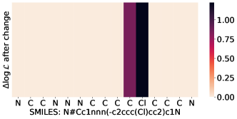
Figure 3: Relative change in vertices pseudo log-likelihood when replacing Cl in the SMILES with an O.

Contrarily to the other baselines, GSPN can answer counterfactual probabilistic queries about the graph as depicted in Figure 3. Here we replace the Chlorine (Cl) atom in the SMILES of an ogbg-molpcba sample with an Oxygen (O) and ask the model to compute again the pseudo log-likelihood of each vertex (Equation 1), therefore answering a “what if” question about the data. In this case, it makes intuitive sense that the relative likelihood increases because Cl is deactivating, so it is more unlikely to observe it attached to the all-carbon atom group. Being able to query the probabilistic model subject to changes in the input naturally confers a degree of interpretability and trustworthiness to the model. For the interested reader, we provide more visualizations for randomly picked samples in Section A.8.

Modeling the Data Distribution under Partial Evidence

We demonstrate that is beneficial to model structural dependencies with GSPN while handling missing values in Table 2. The first observation is that modeling multimodality using a GMM already improves the NLL significantly over the unimodal Gaussian baseline; though this may not seem surprising at first, we stress that this result is a good proxy to measure the usefulness of the datasets selected for this task in terms of difference of attributes, and it establishes an upper bound for the NLL.
Across almost all datasets GSPN improves the NLL score, and we attribute this positive result to its ability to model both the structural dependencies and the multimodality of the data distribution. Interestingly, even when the neighbors do not influence the generation of a vertex attribute (Syn₀), knowing the neighborhood still helps, probably because different communities share similar prior distributions (the choice of the generative parameters and their rationale is discussed in Section A.5). These empirical results seem to agree with the hypotheses of Sections 4.2 (detailed in Section A.5) and shed more light on a research direction worthy of further investigations.

Table 2: We report the mean and std NLL under the missing data scenario, averaged over 3 runs. We report an extended table with more results in Section A.9.

	Syn0	Syn0.5	Syn1	benzene	ethanol	naphthalene	Structure	Multimodal
Gaussian	$5.21\pm 0.0$	$5.21\pm 0.0$	$5.22\pm 0.0$	$7.27\pm 0.0$	$4.57\pm 0.0$	$4.65\pm 0.0$	✗	✗
GMM	$2.97\pm 0.1$	$2.97\pm 0.0$	$2.95\pm 0.0$	$3.81\pm 0.0$	$2.90\pm 0.01$	$2.64\pm 0.06$	✗	✓
GSPNU	$\mathbf{2.92}\pm 0.1$	$\mathbf{2.90}\pm 0.0$	$\mathbf{2.91}$ $\pm$ $0.0$	$\mathbf{3.17}$ $\pm$ $0.02$	$\mathbf{2.87}\pm 0.01$	$\mathbf{2.56}\pm 0.04$	✓	✓

Graph Classification

Table 3: Mean and std results on graph classification datasets. The best and second-best performances are bold and underlined, respectively. A $\dagger$ means that GSPN improves over CGMM.

	NCI1	REDDIT-B	REDDIT-5K	COLLAB
Baseline	$69.8\pm 2.2$	$82.2\pm 3.0$	$52.2\pm 1.5$	$70.2\pm 1.5$
DGCNN	$76.4\pm 1.7$	$87.8\pm 2.5$	$49.2\pm 1.2$	$71.2\pm 1.9$
DiffPool	$76.9\pm 1.9$	$89.1\pm 1.6$	$53.8\pm 1.4$	$68.9\pm 2.0$
ECC	$76.2\pm 1.4$	-	-	-
GIN	$\mathbf{80.0}\pm 1.4$	$89.9\pm 1.9$	$\mathbf{56.1}\pm 1.7$	$75.6\pm 2.3$
GraphSAGE	$76.0\pm 1.8$	$84.3\pm 1.9$	$50.0\pm 1.3$	$73.9\pm 1.7$
CGMMU+DS	$76.2\pm 2.0$	$88.1\pm 1.9$	$52.4\pm 2.2$	$77.3\pm 2.2$
E-CGMMU+DS	$\underline{78.5}\pm 1.7$	$89.5\pm 1.3$	$53.7\pm 1.0$	$77.5\pm 2.3$
iCGMMU+DS	$77.6\pm 1.5$	$\mathbf{91.6}\pm 2.1$	$\underline{55.6}\pm 1.7$	$\mathbf{78.9}\pm 1.7$
GSPNU+DS	${}^{\dagger}76.6\pm 1.9$	${}^{\dagger}\underline{90.5}\pm 1.1$	${}^{\dagger}55.3\pm 2.0$	${}^{\dagger}\underline{78.1}\pm 2.5$
GSPNS	${}^{\dagger}77.6\pm 3.0$	${}^{\dagger}89.7\pm 2.3$	${}^{\dagger}54.2\pm 2.1$	74.1 $\pm$ 2.5

The last quantitative analysis concerns graph classification, whose results are reported in Table 3. As we can see, not only is GSPN competitive against a consistent set of neural and probabilistic DGNs, but it also improves almost always w.r.t. $CGMM$, which can be seen as the layer-wise counterpart of our model. In addition, the model ranks second on two out of five tasks, though there is no clear winner among all models and the average performances are not statistically significant due to high variance. We also observe that here GSPN_S does not bring significant performance gains compared to GSPN_U+DS. As mentioned in Section 4.5, we attribute this to the limited theoretical expressiveness of the global aggregation function.
We also carry out a qualitative analysis on the impact of the number of layers, $C$ and $C_{G}$ for GSPN_S (with global sum pooling) on the different datasets, to shed light on the benefits of different hyper-parameters. The results show that on NCI1 and COLLAB the performance improvement is consistent as we add more layers, whereas the opposite is true for the other two datasets where the performances decrease after five layers. Therefore, the selection of the best number of layers to use remains a non-trivial and dataset-specific challenge. In the interest of space, we report a visualization of these results in Appendix A.10.

7 Conclusions

We have proposed Graph-Induced Sum-Product Networks, a deep and fully probabilistic class of models that can tractably answer probabilistic queries on graph-structured data. GSPN is a composition of locally valid SPNs that mirrors the message-passing mechanism of DGNs, and it works as an unsupervised or supervised model depending on the problem at hand. We empirically demonstrated its efficacy across a diverse set of tasks, such as scarce supervision, modeling the data distribution under missing values, and graph prediction. Its probabilistic nature allows it to answer counterfactual queries on the graph, something that most DGNs cannot do. We hope our contribution will further bridge the gap between probabilistic and neural models for graph-structured data.

Appendix A Appendix

We complement the discussion with theoretical and practical considerations that facilitate understanding and reproducibility.

A.1 High-level Definitions of Probabilistic Circuits

We introduce basic concepts of PCs to ease the understanding of readers that are less familiar with this topic.

A probabilistic circuit [10] over a set of r.v.s $\bm{X}=(A_{1},\dots,A_{d})$ is uniquely determined by its circuit structure and computes a (possibly unnormalized) distribution $P(\bm{X})$. The circuit structure has the form of a rooted DAG, which comprises a set of computational units. In particular, input units are those for which the set of incoming edges is empty (i.e., no children), whereas the output unit has no outgoing edges.

The scope of a PC is a function that associates each unit of the circuit with a subset of $\bm{X}$. For each non-input unit, the scope of the unit is the union of the scope of the children. It follows that the scope of the root is $\bm{X}$.

Each input (or distribution) unit encodes a parametric non-negative function, e.g., a Gaussian or Categorical distribution. A product unit represents the joint, fully factorized distribution between the distributions encoded by its children. Finally, a sum unit defines a weighted sum of the children’s distributions, i.e., a mixture model when the children encode proper distributions. The set of parameters of a probabilistic circuit is given by the union of the parameters of all input and sum units in the circuit.

There are different kinds of probabilistic queries that a PC can answer. The first is the complete evidence query, corresponding to the computation of $P(\bm{X}=\bm{x})$. A single feedforward pass from the input units to the output unit is sufficient to compute this query. Another important class of queries is that of marginals, where we assume that not all r.v.s are fully observed, e.g., missing values. Given partial evidence $\bm{E}\subset\bm{X}$ and the unobserved variables $\bm{Z}=\bm{X}\setminus\bm{E}$, a marginal queries is defined as $P(\bm{E}=\bm{e})=\int p(\bm{e},\bm{z})d\bm{z}$. Finally, we mention the conditional query, sharing the same complexity as the marginal, where we compute the conditional probability $P(\bm{Q}=\bm{q}\mid\bm{E}=\bm{e})$ of a subset of r.v.s $\bm{Q}\subset\bm{X}$ conditioned on partial evidence $\bm{E}$ and $\bm{Z}=\bm{X}\setminus(\bm{E}\cup\bm{Q})$.

To be able to tractably compute the above queries, one usually wants the PC to have specific structural properties that guarantee a linear time complexity for marginal and conditional queries. A product unit is said to be decomposable when the scopes of its children are disjoint, and a PC is decomposable if all its product units are decomposable. Instead, a sum unit is smooth if all its children have identical scopes, and a PC is smooth (or complete [40]) if all its sum units are smooth. For instance, the NB model considered in our work is implemented as a smooth and decomposable PC.

A PC that is smooth and decomposable can tractably compute marginals and conditional queries (one can prove that these are necessary and sufficient conditions for tractable computations of these queries), and we call such SPNs valid. A generalization of decomposability, namely consistency, is necessary to tractably compute maximum a posteriori queries of the form $\arg\max_{\bm{q}}P(\bm{Q}=\bm{q},\bm{E}=\bm{e})$.

PCs have an interpretation in terms of latent variable models [38], and in particular it is possible to augment PCs with specialized input units that mirror the latent variables of the associated graphical model. However, it is not immediate at all to see that valid SPNs allow a tractable computation of the posterior probabilities for the sum units, and we indeed refer the reader to works in the literature that formally prove it. As stated in [40, 38], inference in unconstrained SPNs is generally intractable, but when an SPN is valid efficient inference is possible. Concretely, one can get all the required statistics for computing the posterior probabilities $\bm{h}_{j}$ of any sum unit $j$ in a single backpropagation pass across the SPN (Equation 22 of Peharz et al. [38]). The posterior computation involves the use of tractable quantities and hence stays tractable. Of course, the computational costs depend on the size of the SPN and might be impractical if the SPN is too large, but we still consider it tractable in terms of asymptotic time complexity.

A.2 The Switching Parent decomposition

The decomposition used in Equation 4, known as “Switching Parent” (SP) in the literature [2], was formally introduced in [43] in the context of mixed memory Markov models. We report the original formulation below. Let $i_{t}\in\{1,\dots,n\}$ denote a discrete random variable that can take on $n$ possible values. Then we write the SP decomposition as

$$P(i_{t}\mid i_{t-1},\dots,i_{t-k})=\sum_{\mu=1}^{n}P(\mu)P^{\mu}(i_{t}\mid i_{t-\mu}).$$ (8)

The connection to Equation 4 emerges by observing the following correspondences: $P(\mu)$ is treated as a constant $\frac{1}{|ch_{n}|}$, $P^{\mu}(i_{t}=i\mid i_{t-\mu}=j)$ implements the transition conditional probability table, which we model in a “soft” version (see also [3]) as $\bm{\theta}^{\ell}\bm{h}^{\ell-1}_{u}$, and the conditional variables on the left-hand-side of the equation intuitively correspond to the information $\bm{h}^{\ell-1}_{ch_{n}}$ we use to parametrize the prior $P_{\bm{\pi}^{\ell}}(Q_{v}^{\ell})$. Moreover, we assume full stationarity and ignore the position of the child in the parametrization, meaning we use the same transition weights $\mathbf{\theta}^{\ell}$ for all neighbors; this is crucial since there is usually no consistent ordering of the vertices across different graphs, and consequently between the children in the SPN hierarchy.

A.3 Proof that Equation 4 is a valid parametrization

To show that the computation $\bm{\pi}_{n^{\prime}}^{\ell+1}$ outputs a valid parametrization for the categorical distribution $P_{\bm{\pi}_{n^{\prime}}^{\ell+1}}(Q_{n^{\prime}}^{\ell+1})$, it is sufficient to show that the parameters sum to 1:

$$\sum_{i=1}^{C}\bm{\pi}_{n^{\prime}}^{\ell+1}(i)=\sum_{i=1}^{C}f_{\bm{\theta}^{\ell+1}}(\bm{h}^{\ell}_{1},...,\bm{h}^{\ell}_{|ch_{n^{\prime}}|})_{i} =\sum_{i=1}^{C}\frac{1}{|ch_{n^{\prime}}|}\sum_{n\in ch_{n^{\prime}}}\sum_{k=1}^{C}\bm{\theta}^{\ell+1}_{ki}\bm{h}^{\ell}_{n}(k)$$

$$=\frac{1}{|ch_{n^{\prime}}|}\sum_{n\in ch_{n^{\prime}}}\sum_{k=1}^{C}\sum_{i=1}^{C}\bm{\theta}^{\ell+1}_{ki}\bm{h}^{\ell}_{n}(k)$$

$$=\frac{1}{|ch_{n^{\prime}}|}\sum_{n\in ch_{n^{\prime}}}\sum_{k=1}^{C}\bm{h}^{\ell}_{n}(k)=\frac{1}{|ch_{n^{\prime}}|}\sum_{n\in ch_{n^{\prime}}}1=1,$$ (9)

where we used the fact that the rows of $\bm{\theta}^{\ell}$ and the posterior weights $\bm{h}_{u}^{\ell-1}$ are normalized.

A.4 Dealing with more general SPN templates

In Section 4 we have introduced the general framework of GSPN for arbitrary SPNs, but the explicit implementation of $\bm{\pi}_{n,j}^{\ell}=f_{\bm{\theta}_{j}^{\ell}}(\bm{h}_{n_{1},j}^{\ell-1},\dots,\bm{h}_{n_{T},j}^{\ell-1})$ and the computation of the posterior probabilities $\bm{h}_{n_{i},j}^{\ell-1}$ has only been shown for the Naïve Bayes model (Section 4.1) with a single sum unit $j$ in its corresponding SPN template. Despite that the computation of the posterior depends on the specific template used, we can still provide guidelines on how to use GSPN in the general case.

Consider any valid SPN template with $S$ sum units, and w.l.o.g. we can assume that all sum units have $C$ different weights, i.e., each sum unit implements a mixture of $C$ distributions. Given a computational tree, we consider an internal node $n$ with $T$ children $n_{1},\dots,n_{T}$, and we recall that all SPNs associated with the nodes of the tree share the same template (although a different parametrization). Therefore, there is a one-to-one correspondence between unit $j$ of node $n_{i},\ \forall i\in\{1,\dots,T\}$, at level $\ell-1$ and unit $j$ of its parent $n$ at level $\ell$, meaning that the parametrization $\bm{\pi}_{n,j}^{\ell}\in\mathbb{R}^{C}$ can be computed using a permutation invariant function such as

$$\bm{\pi}_{n,j}^{\ell}=f_{\bm{\theta}_{j}^{\ell}}(\bm{h}_{n_{1},j}^{\ell-1},\dots,\bm{h}_{n_{T},j}^{\ell-1})=\frac{1}{T}\sum_{i=1}^{T}\bm{\theta}_{j}^{\ell}\bm{h}^{\ell-1}_{n_{i},j}\ \ \ \ \forall j\in\{1,\dots,S\}$$ (10)

that acts similarly to the neighborhood aggregation function of DGNs.

All that remains is to describe how we compute the posterior probabilities $\bm{h}^{\ell}_{n,j}\in\mathbb{R}^{C}$ for all sum units $j\in\{1,\dots,S\}$ of a generic node $n$ at level $\ell$ (now that the reader is familiar with the notation, we can abstract from the superscript $\ell$ since it can be determined from $n$). As discussed in Section A.1, SPNs have an interpretation in terms of latent variable models, so we can think of a sum unit $j$ as a latent random variable and we can augment the SPN to make this connection explicit [38]. Whenever the SPN is valid, the computation of the posterior probabilities of all sum units is tractable and it requires just one backpropagation pass across the augmented SPN (see Equation 22 of Peharz et al. [38]). This makes it possible to tractably compute the posterior probabilities of the sum units that will be used to parametrize the corresponding sum units of the parent node in the computational tree. Below we provide a pseudocode summarizing the inference process for a generic GSPN, but we remind the reader that the message passing procedure is equivalent to that of DGNs.

Algorithm 1 GSPN Inference on a Single Computational Tree

Input: Computational tree with $T$ nodes and height $L$, valid SPN template with $S$ sum units
                  and $C$ weights for each sum unit.
      Output: Set of posterior probabilities $\{\bm{h}_{n,j}\ \ \forall n\in\{1,\dots,T\},\forall j\in\{1,\dots,S\}\}$

1:for $\ell=0,\ldots,L$ do

2:     for all nodes $n$ at height $\ell$ do

3:         for all sum units $j$ of SPN of node $n$ do:

4:              if $\ell>0$ then:

5:                  Compute $\bm{\pi}_{n,j}$ (Eq. 10) $\triangleright$ message passing, parallelized

6:              else

7:                  Use learned $\bm{\pi}_{n,j}$ $\triangleright$ leaf node, no children

8:              end if

9:              Compute and collect $\bm{h}_{n,j}$ (Equation 22 [38]) $\triangleright$ computation reused across sum units

10:         end for

11:     end for

12:end for

13:return $\{\bm{h}_{n,j}\ \ \forall n\in\{1,\dots,T\},\forall j\in\{1,\dots,S\}\}$

On a separate note, when it comes to handling missing data, it is sufficient to marginalize out the missing evidence by substituting a $1$ in place of the missing input units. This allows us to compute any marginal or conditional query (including the computation of the posterior probabilities) in the presence of partial evidence.

A.5 Details of the synthetic datasets’ generative process

The study of attributed graph generation has gained traction in recent years [39, 34, 62, 45]. When it comes to the imputation of missing vertex attributes in graphs, we identified specific and challenging conditions under which GSPN can be advantageous compared to both structure-agnostic models, e.g., a Gaussian Mixture Model (GMM), and structure-aware neighbor aggregators. First, the distribution of attributes should be multimodal, so that a simple neural neighbor aggregator is unable to produce it. Second, the attributes should be independent, i.e., there is no correlation, meaning knowledge of one attribute value cannot be used to impute another. Finally, the generation of node attributes depends on the neighbors, so a GMM cannot capture such information.

Below, we detail the process through which we generate synthetic samples for the missing data imputation experiments.

Graph Generation

Each generated graph contains $5$ communities for a total random number of vertices $\in[50,100]$. The intra-community (respectively inter-community) edge probability is uniformly sampled in the range $[0.01,0.1]$ ($[0.0001,0.001]$), to ensure topological variability and some mixing of communities.

Attribute Generation

Following the discussion of Section 4.2, we first generate a graph structure and use it to generate structure-dependent vertex attributes. Given a set of vertices $\mathcal{V}$ and edges $\mathcal{E}$ generated by the SBM, we sample each vertex attribute from a Gaussian mixture model with 3 components, whose prior distribution can be influenced by the neighborhood of each vertex. If we consider a function $c:\mathcal{V}\rightarrow\{1,\dots,5\}$ that maps each vertex to its SBM community, the generative process is defined as

$$\mu_{i}\sim\mathcal{U}[-100,100],\ \ \forall i\in{1,2,3}$$ (11)

$$\sigma_{i}\sim\mathcal{U}[0,5],\ \ \forall i\in{1,2,3}$$ (12)

$$\pi_{v}\sim Dir(\bm{\alpha}_{c(v)}),\ \bm{\alpha}_{c(v)}\in\mathbb{R}^{3},\forall v\in\mathcal{V}$$ (13)

$$\pi_{\mathcal{N}_{v}}=\frac{\sum_{u\in\mathcal{N}_{v}}\pi_{u}}{|\mathcal{N}_{v}|}$$ (14)

$$\bm{X}_{v}\sim\sum_{i}(\lambda_{v}\pi_{v}+\lambda_{\mathcal{N}_{v}}\pi_{\mathcal{N}_{v}})\mathcal{N}(\mu_{i},\sigma_{i}),$$ (15)

noting that each $\bm{\alpha}_{c(v)}$ (one per community) has been designed in such a way that different communities have different prior distributions. In particular, the chosen parameters are (using a matrix $\bm{\alpha}$ $\in R^{5\times 3}$):

$$\text{\huge$\bm{\alpha}$}=\begin{bmatrix}9.&1.&1.\\ 1.&9.&1.\\ 1.&1.&9.\\ 2.&2.&1.\\ 1.&1.&2.\end{bmatrix}.$$ (16)

The constants $\lambda_{v}$ and $\lambda_{\mathcal{N}_{v}}$, which must sum to 1, control the dependence of the vertex attribute on the surrounding neighbors. A $\lambda_{v}=1$ means that the structure does not influence at all the vertex generation; here a GMM is expected to work well. In contrast, $\lambda_{\mathcal{N}_{v}}=1$ strongly promotes interdependence between adjacent vertices in terms of similar attribute values. To simulate multi-modality, once a graph structure and its clustering weights have been sampled we repeat sampling of vertex attributes $100$ times using Equation 15. Starting from $100$ different SBM graphs, we create a total of 10000 synthetic graphs. We generate three different datasets according to the chosen value for $\lambda_{\mathcal{N}_{v}}\in[0,0.5,1]$.

A.6 Hyper-parameters tried during model selection

The following tables report the hyper-parameters tried during model selection.

Table 4: Scarce supervision experiments. We found that too large batch sizes caused great instability in GIN’s training, so we tried different, smaller options. DGI and GAE used the Atom Embedder of size 100 provided by OGBG, whereas GSPN deals with categorical attributes through a Categorical distribution. The range of hyper-parameters tried for GAE and DGI follows previous works.

	Embedding Construction
	$C$ / latent dim	# layers	learning rate	batch size	# epochs	ES patience	avg emission params across layers
GAE	32, 128, 256	2,3,5	0,1, 0.01	1024	100	50
DGI	32, 128, 256	2,3,5	0,1, 0.01	1024	100	50
GSPN	5,10,20,40	5,10,20	0.1	1024	100	50	true, false
	Graph Predictor
							global pooling	w. decay (MLP) dropout (GIN)
MLP	8,16,32,64	1	0.01	1024	1000	500	sum, mean	0, 0.0001
GIN	32,256,512	2,5	0.01, 0.0001	8,32,128	1000	500	sum, mean	0., 0.5

Table 5: Missing data experiments. Gaussian mixtures of distributions are initialized with k-means on the first batch of the training set. The maximum variance at initialization is set to 10.

	$C$	# layers	learning rate	batch size	# epochs	ES patience	avg emission params across layers
Gaussian	-	-	-	-	-	-	-
GMM	5,15,20,40	1	0,1, 0.01	32	200	50	-
GSPN	5,15,20,40	2	0,1, 0.01	32	200	50	false

Table 6: Graph classification experiments. The emission distribution is categorical for NCI1 and univariate Gaussian otherwise. Gaussian mixtures of distributions to be learned (social datasets) are initialized using k-means on the training set.

	Embedding Construction
	$C$ / latent dim	# layers	learning rate	batch size	# epochs	ES patience	avg emission params across layers
GSPNU	5,10,20	5, 10, 15, 20	0,1	32	500	50	true, false
	Graph Predictor
							global pooling
MLP	8, 16, 32, 128	1	0.001	32	1000	200	sum, mean
GSPNS	$C$=5,10,20 $C_{g}$=32,128	1	0.001	32	1000	200	sum, mean

A.7 Datasets Statistics

Below we report the set of datasets used in our work together with their characteristics.

Table 7: Dataset statistics.

	# graphs	# vertices	# edges	# vertex attributes	task	metric
benzene	527984	12.00	64.94	1 categorical + 6 cont.	Regression(1)	MAE/NLL
ethanol	455093	9.00	36.00	3 (1 cat.) + 6 cont.	Regression(1)	MAE/NLL
naphthalene	226256	18.00	127.37	3 (1 cat.) + 6 cont.	Regression(1)	MAE/NLL
salicylic acid	220232	16.00	104.13	3 (1 cat.) + 6 cont.	Regression(1)	MAE/NLL
toluene	342791	15.00	96.15	3 (1 cat.) + 6 cont.	Regression(1)	MAE/NLL
malonaldehyde	893238	9.00	36.00	3 (1 cat.) + 6 cont.	Regression(1)	MAE/NLL
uracil	133770	12.00	64.44	4 (1 cat.) + 6 cont.	Regression(1)	MAE/NLL
ogbg-molpcba	437929	26.0	28.1	83 (9 cat.)	Multi-Label Classification(128)	AP
Syn∗	10000	71.23	367.48	1 cont.	PDE, Reconstruction(1)	NLL, MSE
NCI1	4110	29.87	32.30	37 (1 cat.)	Classification(2)	ACC
REDDIT-B	2000	429.63	497.75	1 cont.	Classification(2)	ACC
REDDIT-5K	5000	508.52	594.87	1 cont.	Classification(5)	ACC
COLLAB	5000	74.49	2457.78	1 cont.	Classification(3)	ACC

A.8 Scarce Supervision Experiments: Additional Visualizations

Figure 5 provides a few, randomly picked examples of molecules from the ogbg-molpcba dataset, modified to show the relative change in log-likelihood of some of the vertices according to GSPN.

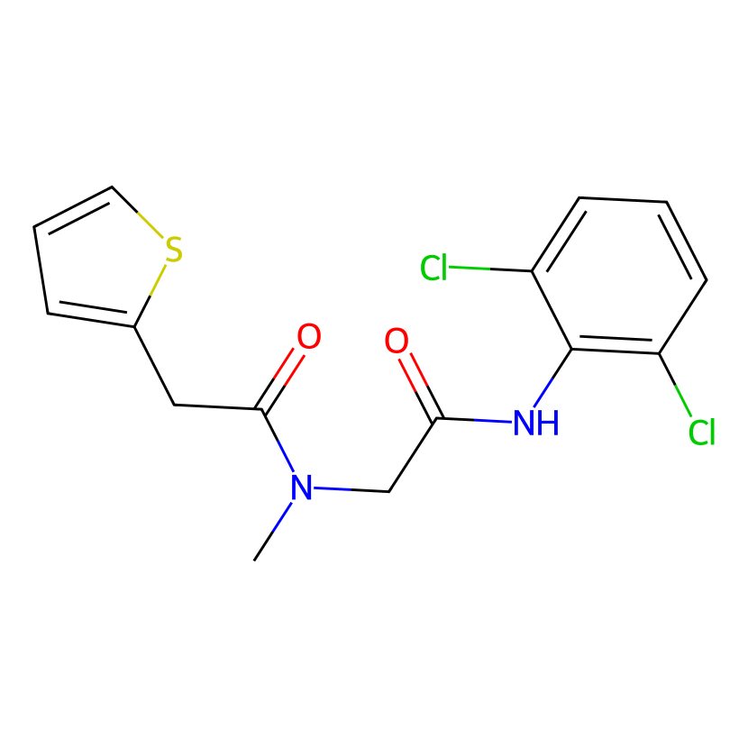
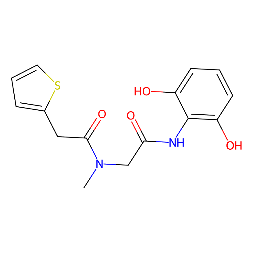
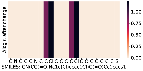
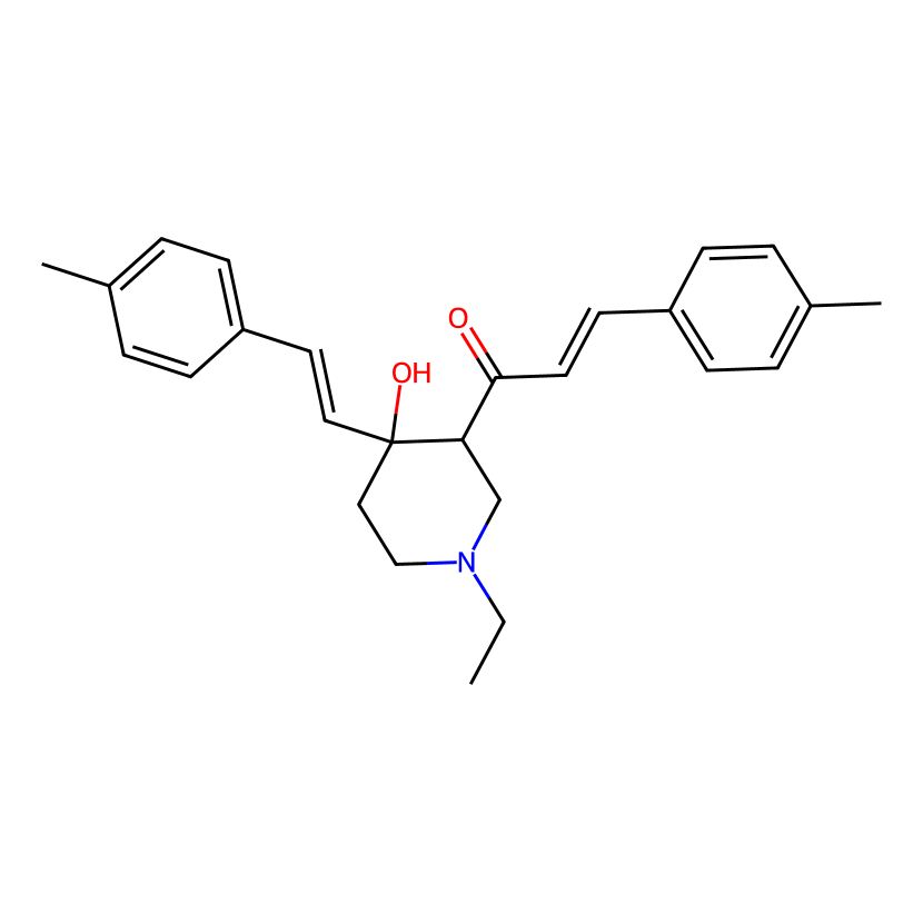
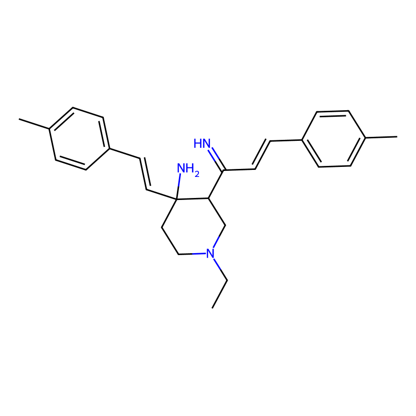
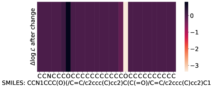
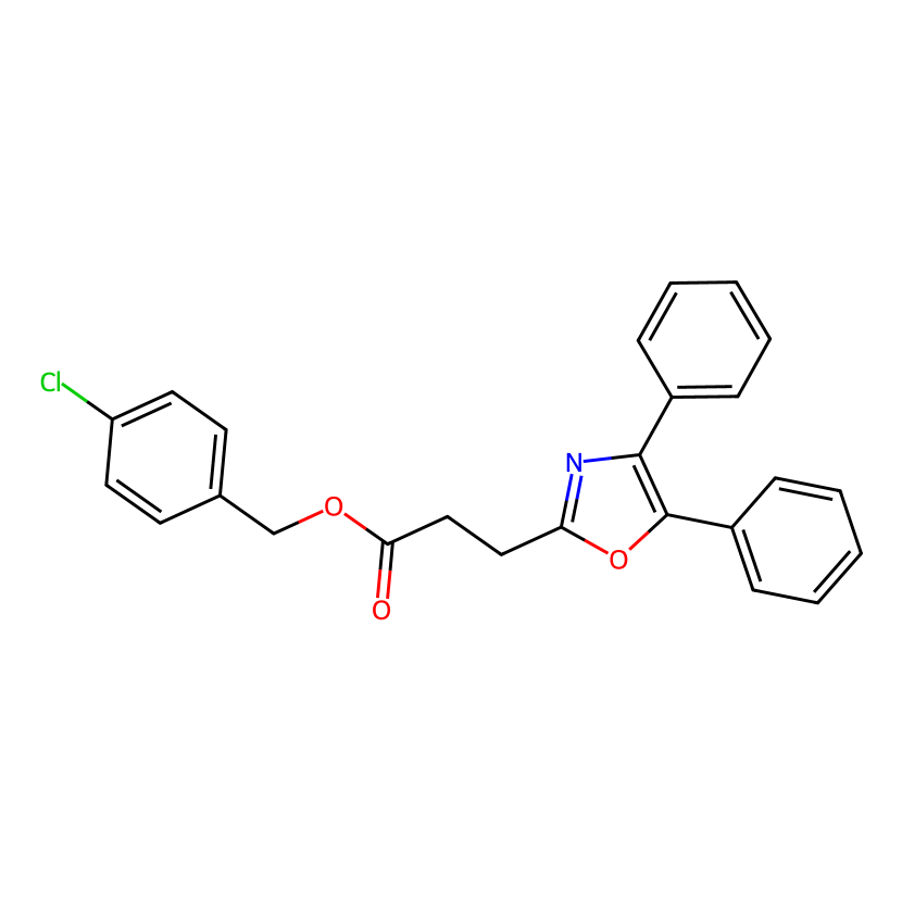
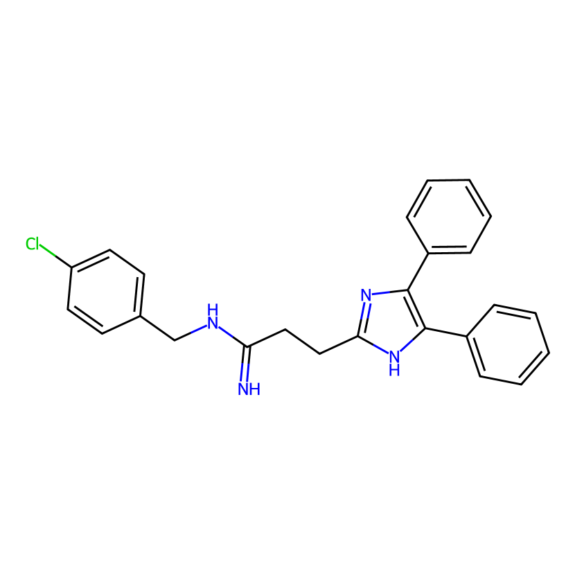
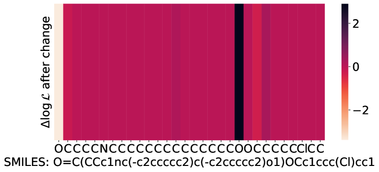
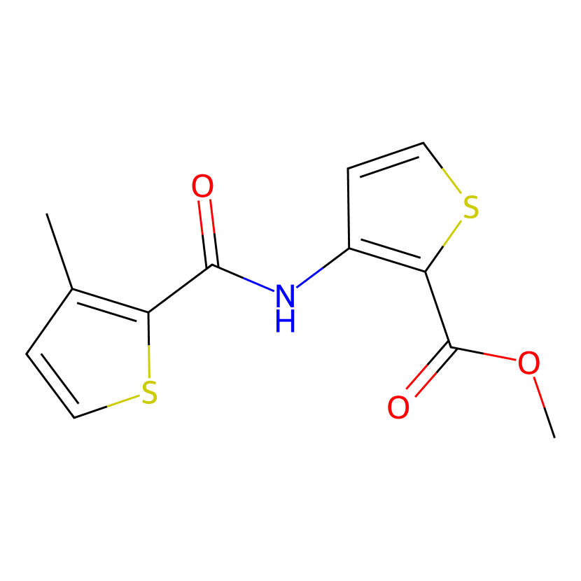
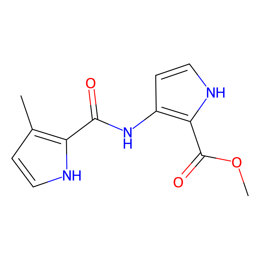
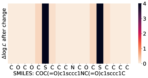
Figure 5: Additional visualizations of randomly picked molecules from ogbg-molpcba for a specific GSPN configuration. The heatmap shows log-likelihood variations in the vertices when operating specific atomic changes (from left to right). Nearby atoms are affected by the change as well, and this allows us to understand which groups are more common, or make more sense, than others.

A.9 Missing Data Experiments: Additional Results

We extend the results of Table 2 with the other chemical datasets with continuous attributes.

Table 8: We report additional results for the missing data experiments, where we show that GSPN can incorporate the graph structure to better model the data distribution under missing data. We report the mean and std NLL across $3$ final (i.e., after model selection) training runs.

	Gaussian	GMM	GSPNU
benzene	$7.27\pm 0.0$	$3.81\pm 0.0$	$\mathbf{3.17}\pm 0.02$
ethanol	$4.57\pm 0.0$	$2.90\pm 0.01$	$\mathbf{2.87}\pm 0.01$
malonaldehyde	$4.70\pm 0.0$	$2.99\pm 0.0$	$\mathbf{2.96}\pm 0.0$
naphthalene	$4.65\pm 0.0$	$2.64\pm 0.06$	$\mathbf{2.56}\pm 0.04$
salicylic acid	$4.55\pm 0.0$	$2.61\pm 0.06$	$\mathbf{2.51}\pm 0.11$
toluene	$4.81\pm 0.0$	$2.85\pm 0.03$	$\mathbf{2.70}\pm 0.02$
uracil	$4.45\pm 0.0$	$\mathbf{2.54}\pm 0.07$	$2.56\pm 0.15$

A.10 Graph Classification Experiments: Ablation and Hyper-parameter Studies

Ablation Study

The following table shows the performance of GSPN_U+DS when removing the use shortcut connections from the hyper-parameter space. The results show that using shortcut connections consistently leads to better mean classification accuracy on these tasks.

Table 9: Impact of shortcut connections on the creation of unsupervised embeddings for graph classification.

	NCI1	REDDIT-B	REDDIT-5K	COLLAB
GSPN${}_{U+DS}\mbox{ (no shortcut)}$	$76.5\pm 1.9$	$88.9\pm 3.9$	$52.3\pm 5.2$	$75.7\pm 2.6$
GSPNU+DS	$76.6\pm 1.9$	$90.5\pm 1.1$	$55.3\pm 2.0$	$78.1\pm 2.5$

Impact of Hyper-parameters

Figure 6 shows how the validation performance of GSPN_S changes for specific hyper-parameters $C$ and $C_{G}$ as we add more layers. Please refer to the main text for a discussion.

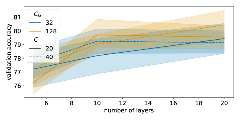
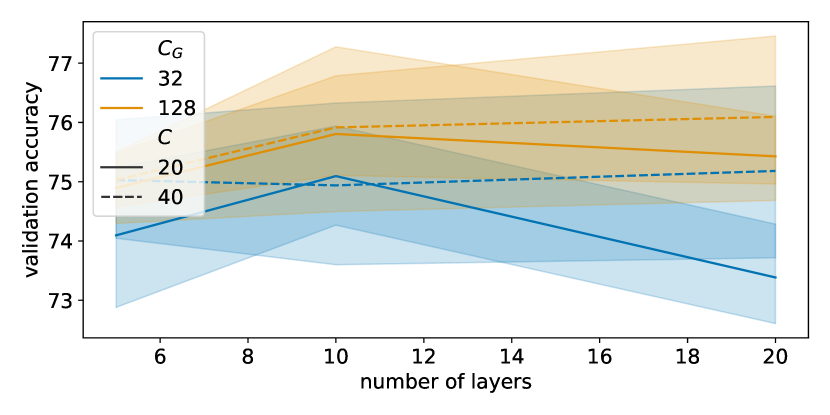
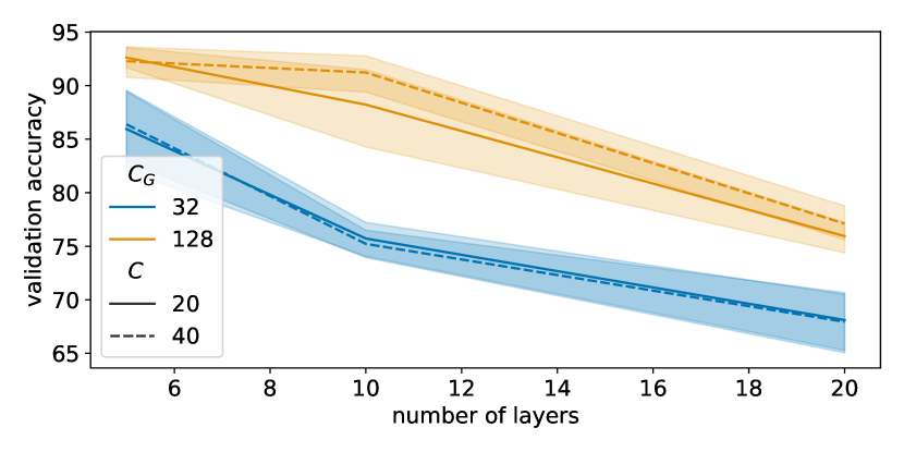
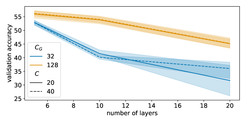
Figure 6: Impact of GSPN_S layers, $C$ and $C_{G}$ on NCI1 (top left), COLLAB (top right), REDDIT-BINARY (bottom left), and REDDIT-5K (bottom right) performances, averaged across all configurations in the 10 outer folds.

A.11 Time Comparison

Table 10 shows the time comparison of forward and backward passes on a batch of size 32 between GSPN and GIN. We used 10 layers for both architectures and adapted the hidden dimensions to obtain a comparable number of parameters. Despite the GIN’s implementation being more sample efficient than GSPN, the table confirms our claims on the asymptotic complexity of GSPN.

Table 10: Time comparison between GSPN and GIN on graph classification tasks.

	# parameters		forward time (ms)		backward time (ms)
	GSPN	GIN	GSPN	GIN	GSPN	GIN
NCI1	36876	36765	30	12	17	14
REDDIT-B	34940	35289	35	14	24	15
REDDIT-5K	34940	35289	35	14	22	15
COLLAB	34940	35289	36	14	21	15

References

- Atzeni et al. [2021] Daniele Atzeni, Davide Bacciu, Federico Errica, and Alessio Micheli. Modeling edge features with deep bayesian graph networks. In Proceedings of the International Joint Conference on Neural Networks (IJCNN), 2021.
- Bacciu et al. [2010] Davide Bacciu, Alessio Micheli, and Alessandro Sperduti. Bottom-up generative modeling of tree-structured data. In Proceedings of the 17th International Conference on Neural Information Processing (ICONIP), 2010.
- Bacciu et al. [2020a] Davide Bacciu, Federico Errica, and Alessio Micheli. Probabilistic learning on graphs via contextual architectures. Journal of Machine Learning Research, 21(134):1–39, 2020a.
- Bacciu et al. [2020b] Davide Bacciu, Federico Errica, Alessio Micheli, and Marco Podda. A gentle introduction to deep learning for graphs. Neural Networks, 129:203–221, 9 2020b.
- Bishop [2006] Christopher M Bishop. Pattern recognition and machine learning. Springer, 2006.
- Bronstein et al. [2017] Michael M. Bronstein, Joan Bruna, Yann LeCun, Arthur Szlam, and Pierre Vandergheynst. Geometric deep learning: going beyond Euclidean data. IEEE Signal Processing Magazine, 34(4):25. 18–42, 2017.
- Castellana et al. [2022] Daniele Castellana, Federico Errica, Davide Bacciu, and Alessio Micheli. The infinite contextual graph Markov model. In Proceedings of the 39th International Conference on Machine Learning (ICML), 2022.
- Chen et al. [2022] Xu Chen, Siheng Chen, Jiangchao Yao, Huangjie Zheng, Ya Zhang, and Ivor W. Tsang. Learning on Attribute-Missing Graphs. IEEE Transactions on Pattern Analysis and Machine Intelligence, 44(2):740–757, 2022.
- Chmiela et al. [2017] Stefan Chmiela, Alexandre Tkatchenko, Huziel E Sauceda, Igor Poltavsky, Kristof T Schütt, and Klaus-Robert Müller. Machine learning of accurate energy-conserving molecular force fields. Science advances, 3(5):e1603015, 2017.
- Choi et al. [2020] YooJung Choi, Antonio Vergari, and Guy Van den Broeck. Probabilistic circuits: A unifying framework for tractable probabilistic models. Preprint, 2020.
- Darwiche [2003] Adnan Darwiche. A differential approach to inference in bayesian networks. Journal of the ACM (JACM), 50(3):280–305, 2003.
- Dempster et al. [1977] Arthur P Dempster, Nan M Laird, and Donald B Rubin. Maximum likelihood from incomplete data via the em algorithm. Journal of the Royal Statistical Society: Series B (Methodological), 39(1):1–22, 1977.
- Erhan et al. [2010] Dumitru Erhan, Aaron Courville, Yoshua Bengio, and Pascal Vincent. Why does unsupervised pre-training help deep learning? In Proceedings of the 13th International Conference on Artificial Intelligence and Statistics (AISTATS), 2010.
- Errica et al. [2020] Federico Errica, Marco Podda, Davide Bacciu, and Alessio Micheli. A fair comparison of graph neural networks for graph classification. In 8th International Conference on Learning Representations (ICLR), 2020.
- Frasconi et al. [1998] Paolo Frasconi, Marco Gori, and Alessandro Sperduti. A general framework for adaptive processing of data structures. IEEE Transactions on Neural Networks, 9(5):768–786, 1998.
- Gens and Domingos [2012] Robert Gens and Pedro Domingos. Discriminative learning of sum-product networks. Proceedings of the 26th Conference on Neural Information Processing Systems (NeurIPS), 2012.
- Gepperth and Pfülb [2021] Alexander Gepperth and Benedikt Pfülb. Gradient-based training of gaussian mixture models for high-dimensional streaming data. Neural Processing Letters, 53(6):4331–4348, 2021.
- Gilmer et al. [2017] Justin Gilmer, Samuel S Schoenholz, Patrick F Riley, Oriol Vinyals, and George E Dahl. Neural message passing for quantum chemistry. In Proceedings of the 34th International Conference on Machine Learning (ICML), pages 1263–1272, 2017.
- Hamilton et al. [2017a] Will Hamilton, Zhitao Ying, and Jure Leskovec. Inductive representation learning on large graphs. In Proceedings of the 31st Conference on Neural Information Processing Systems (NIPS), 2017a.
- Hamilton et al. [2017b] William L. Hamilton, Rex Ying, and Jure Leskovec. Representation learning on graphs: Methods and applications. IEEE Data Engineering Bulletin, 40(3):52–74, 2017b.
- Hao et al. [2020] Zhongkai Hao, Chengqiang Lu, Zhenya Huang, Hao Wang, Zheyuan Hu, Qi Liu, Enhong Chen, and Cheekong Lee. Asgn: An active semi-supervised graph neural network for molecular property prediction. In Proceedings of the 26th International Conference on Knowledge Discovery and Data Mining (SIGKDD, 2020.
- He et al. [2016] Kaiming He, Xiangyu Zhang, Shaoqing Ren, and Jian Sun. Deep residual learning for image recognition. In Proceedings of the 29th IEEE Conference on Computer Vision and Pattern Recognition (CVPR), 2016.
- Holland et al. [1983] Paul W Holland, Kathryn Blackmond Laskey, and Samuel Leinhardt. Stochastic blockmodels: First steps. Social networks, 5(2):109–137, 1983.
- Hu et al. [2020a] Weihua Hu, Matthias Fey, Marinka Zitnik, Yuxiao Dong, Hongyu Ren, Bowen Liu, Michele Catasta, and Jure Leskovec. Open graph benchmark: Datasets for machine learning on graphs. In Proceedings of the 34th Conference on Neural Information Processing Systems (NeurIPS), 2020a.
- Hu et al. [2020b] Weihua Hu, Bowen Liu, Joseph Gomes, Marinka Zitnik, Percy Liang, Vijay Pande, and Jure Leskovec. Strategies for pre-training graph neural networks. In 8th International Conference on Learning Representations (ICLR), 2020b.
- Hüllermeier and Waegeman [2021] Eyke Hüllermeier and Willem Waegeman. Aleatoric and epistemic uncertainty in machine learning: An introduction to concepts and methods. Machine Learning, 110(3):457–506, 2021.
- Hunt and Jorgensen [2003] Lynette Hunt and Murray Jorgensen. Mixture model clustering for mixed data with missing information. Computational statistics & data analysis, 41(3-4):429–440, 2003.
- Kipf and Welling [2016] Thomas N Kipf and Max Welling. Variational graph auto-encoders. In Workshop on Bayesian Deep Learning, Neural Information Processing System (NIPS), 2016.
- Kipf and Welling [2017] Thomas N Kipf and Max Welling. Semi-supervised classification with graph convolutional networks. In 5th International Conference on Learning Representations (ICLR), 2017.
- Koller and Friedman [2009] Daphne Koller and Nir Friedman. Probabilistic graphical models: principles and techniques. MIT press, 2009.
- Malone et al. [2021] Brandon Malone, Alberto Garcia-Duran, and Mathias Niepert. Learning representations of missing data for predicting patient outcomes. In Workshop on Deep Learning on Graphs: Method and Applications (AAAI), 2021.
- Mena et al. [2021] José Mena, Oriol Pujol, and Jordi Vitrià. A survey on uncertainty estimation in deep learning classification systems from a bayesian perspective. ACM Computing Surveys (CSUR), 54(9):1–35, 2021.
- Micheli [2009] Alessio Micheli. Neural network for graphs: A contextual constructive approach. IEEE Transactions on Neural Networks, 20(3):498–511, 2009.
- Mussmann et al. [2015] Stephen Mussmann, John Moore, Joseph Pfeiffer, and Jennifer Neville. Incorporating assortativity and degree dependence into scalable network models. In Proceedings of the 29th AAAI Conference on Artificial Intelligence (AAAI), 2015.
- Niepert et al. [2016] Mathias Niepert, Mohamed Ahmed, and Konstantin Kutzkov. Learning convolutional neural networks for graphs. In Proceedings of the 33th International Conference on Machine Learning (ICML), 2016.
- Palowitch et al. [2022] John Palowitch, Anton Tsitsulin, Brandon Mayer, and Bryan Perozzi. Graphworld: Fake graphs bring real insights for gnns. In Proceedings of the 28th International Conference on Knowledge Discovery and Data Mining (SIGKDD, 2022.
- Pearl [2009] Judea Pearl. Causality. Cambridge university press, 2009.
- Peharz et al. [2016] Robert Peharz, Robert Gens, Franz Pernkopf, and Pedro Domingos. On the latent variable interpretation in sum-product networks. IEEE transactions on pattern analysis and machine intelligence, 39(10):2030–2044, 2016.
- Pfeiffer III et al. [2014] Joseph J Pfeiffer III, Sebastian Moreno, Timothy La Fond, Jennifer Neville, and Brian Gallagher. Attributed graph models: Modeling network structure with correlated attributes. In Proceedings of the 23rd international conference on World Wide Web (WWW), 2014.
- Poon and Domingos [2011] Hoifung Poon and Pedro Domingos. Sum-product networks: A new deep architecture. In IEEE International Conference on Computer Vision (ICCV), Workshops, pages 689–690. IEEE, 2011.
- Qu et al. [2019] Meng Qu, Yoshua Bengio, and Jian Tang. GMNN: Graph Markov Neural Networks. In Proceedings of the 36th International Conference on Machine Learning (ICML), 2019.
- Rossi et al. [2022] Emanuele Rossi, Henry Kenlay, Maria I. Gorinova, Benjamin Paul Chamberlain, Xiaowen Dong, and Michael M. Bronstein. On the unreasonable effectiveness of feature propagation in learning on graphs with missing node features. In Proceedings of the 1st Learning on Graphs Conference (LoG), 2022.
- Saul and Jordan [1999] Lawrence K Saul and Michael I Jordan. Mixed memory Markov models: Decomposing complex stochastic processes as mixtures of simpler ones. Machine Learning, 37(1):75–87, 1999.
- Scarselli et al. [2009] Franco Scarselli, Marco Gori, Ah Chung Tsoi, Markus Hagenbuchner, and Gabriele Monfardini. The graph neural network model. IEEE Transactions on Neural Networks, 20(1):61–80, 2009.
- Shah et al. [2019] Harshay Shah, Suhansanu Kuma, and Hari Sundaram. Growing attributed networks through local processes. In Proceedings of the 28th international conference on World Wide Web (WWW), 2019.
- Shao et al. [2020] Xiaoting Shao, Alejandro Molina, Antonio Vergari, Karl Stelzner, Robert Peharz, Thomas Liebig, and Kristian Kersting. Conditional sum-product networks: Imposing structure on deep probabilistic architectures. In Proceedings of the 9th International Conference on Probabilistic Graphical Models (PGM), 2020.
- Sharir et al. [2016] Or Sharir, Ronen Tamari, Nadav Cohen, and Amnon Shashua. Tensorial mixture models. arXiv preprint arXiv:1610.04167, 2016.
- Simonovsky and Komodakis [2017] Martin Simonovsky and Nikos Komodakis. Dynamic edge-conditioned filters in convolutional neural networks on graphs. In Proceedings of the IEEE Conference on Computer Vision and Pattern Recognition (CVPR), 2017.
- Srivastava et al. [2015] Rupesh Kumar Srivastava, Klaus Greff, and Jürgen Schmidhuber. Highway networks. In Deep Learning Workshop, 32nd International Conference on Machine Learning (ICML), 2015.
- Taguchi et al. [2021] Hibiki Taguchi, Xin Liu, and Tsuyoshi Murata. Graph Convolutional Networks for Graphs Containing Missing Features. Future Generation Computer Systems, 117:155–168, April 2021. ISSN 0167739X. doi: 10.1016/j.future.2020.11.016. URL http://arxiv.org/abs/2007.04583.
- Tajbakhsh et al. [2020] Nima Tajbakhsh, Laura Jeyaseelan, Qian Li, Jeffrey N Chiang, Zhihao Wu, and Xiaowei Ding. Embracing imperfect datasets: A review of deep learning solutions for medical image segmentation. Medical Image Analysis, 63:101693, 2020.
- Trapp et al. [2019] Martin Trapp, Robert Peharz, Hong Ge, Franz Pernkopf, and Zoubin Ghahramani. Bayesian learning of sum-product networks. Proceedings of the 33rd Conference on Neural Information Processing Systems (NeurIPS), 2019.
- Velickovic et al. [2018] Petar Velickovic, Guillem Cucurull, Arantxa Casanova, Adriana Romero, Pietro Lio, and Yoshua Bengio. Graph attention networks. In 6th International Conference on Learning Representations (ICLR), 2018.
- Velickovic et al. [2019] Petar Velickovic, William Fedus, William L. Hamilton, Pietro Liò, Yoshua Bengio, and R. Devon Hjelm. Deep Graph Infomax. In 7th International Conference on Learning Representations (ICLR), New Orleans, LA, USA, May 6-9, 2019, 2019.
- Vergari et al. [2019a] Antonio Vergari, Nicola Di Mauro, and Floriana Esposito. Visualizing and understanding sum-product networks. Machine Learning, 108(4):551–573, 2019a.
- Vergari et al. [2019b] Antonio Vergari, Alejandro Molina, Robert Peharz, Zoubin Ghahramani, Kristian Kersting, and Isabel Valera. Automatic bayesian density analysis. In Proceedings of the 33rd AAAI Conference on Artificial Intelligence (AAAI), pages 5207–5215, 2019b.
- Wale et al. [2008] Nikil Wale, Ian A Watson, and George Karypis. Comparison of descriptor spaces for chemical compound retrieval and classification. Knowledge and Information Systems, 14(3):347–375, 2008.
- Webb et al. [2010] Geoffrey I Webb, Eamonn Keogh, and Risto Miikkulainen. Naïve bayes. Encyclopedia of machine learning, 15:713–714, 2010.
- Wu et al. [2020] Zonghan Wu, Shirui Pan, Fengwen Chen, Guodong Long, Chengqi Zhang, and S Yu Philip. A comprehensive survey on graph neural networks. IEEE Transactions on Neural Networks and Learning Systems, 2020.
- Xu et al. [2019] Keyulu Xu, Weihua Hu, Jure Leskovec, and Stefanie Jegelka. How powerful are graph neural networks? In 7th International Conference on Learning Representations (ICLR), 2019.
- Xu and Jordan [1996] Lei Xu and Michael I Jordan. On convergence properties of the em algorithm for gaussian mixtures. Neural computation, 8(1):129–151, 1996.
- Yamaguchi and Hayashi [2017] Yuto Yamaguchi and Kohei Hayashi. When does label propagation fail? a view from a network generative model. In Proceedings of the 26th International Joint Conference on Artificial Intelligence (IJCAI), 2017.
- Yanardag and Vishwanathan [2015] Pinar Yanardag and SVN Vishwanathan. Deep graph kernels. In Proceedings of the 21th International Conference on Knowledge Discovery and Data Mining (SIGKDD, 2015.
- Ying et al. [2021] Chengxuan Ying, Tianle Cai, Shengjie Luo, Shuxin Zheng, Guolin Ke, Di He, Yanming Shen, and Tie-Yan Liu. Do transformers really perform badly for graph representation? In Proceedings of the 35th Conference on Neural Information Processing Systems (NeurIPS), 2021.
- Ying et al. [2018] Zhitao Ying, Jiaxuan You, Christopher Morris, Xiang Ren, Will Hamilton, and Jure Leskovec. Hierarchical graph representation learning with differentiable pooling. In Proceedings of the 32nd Conference on Neural Information Processing Systems (NeurIPS), 2018.
- Zaheer et al. [2017] Manzil Zaheer, Satwik Kottur, Siamak Ravanbakhsh, Barnabas Poczos, Ruslan R Salakhutdinov, and Alexander J Smola. Deep sets. In Proceedings of the 31st Conference on Neural Information Processing Systems (NIPS), 2017.
- Zhang et al. [2018a] Muhan Zhang, Zhicheng Cui, Marion Neumann, and Yixin Chen. An end-to-end deep learning architecture for graph classification. In Proceedings of the 32nd AAAI Conference on Artificial Intelligence (AAAI), 2018a.
- Zhang et al. [2018b] Ziwei Zhang, Peng Cui, and Wenwu Zhu. Deep learning on graphs: A survey. arXiv preprint arXiv:1812.04202, 2018b.
- Zio et al. [2007] Marco Di Zio, Ugo Guarnera, and Orietta Luzi. Imputation through finite gaussian mixture models. Computational Statistics and Data Analysis, 51(11):5305–5316, 2007. doi: 10.1016/j.csda.2006.10.002.