Iteratively Learning Representations for Unseen Entities with Inter-Rule Correlations

Abstract.

Recent work on knowledge graph completion (KGC) focuses on acquiring embeddings of entities and relations in knowledge graphs. These embedding methods necessitate that all test entities be present during the training phase, resulting in a time-consuming retraining process for out-of-knowledge-graph (OOKG) entities. To tackle this predicament, current inductive methods employ graph neural networks to represent unseen entities by aggregating information of the known neighbors, and enhance the performance with additional information, such as attention mechanisms or logic rules. Nonetheless, Two key challenges continue to persist: (i) identifying inter-rule correlations to further facilitate the inference process, and (ii) capturing interactions among rule mining, rule inference, and embedding to enhance both rule and embedding learning.

In this paper, we propose a virtual neighbor network with inter-rule correlations (VNC) to address the above challenges. VNC consists of three main components: (i) rule mining, (ii) rule inference, and (iii) embedding. To identify useful complex patterns in knowledge graphs, both logic rules and inter-rule correlations are extracted from knowledge graphs based on operations over relation embeddings. To reduce data sparsity, virtual networks for OOKG entities are predicted and assigned soft labels by optimizing a rule-constrained problem. We also devise an iterative framework to capture the underlying interactions between rule and embedding learning. Experimental results on both link prediction and triple classification tasks show that the proposed VNC framework achieves state-of-the-art performance on four widely-used knowledge graphs. Our code and data are available at https://github.com/WZH-NLP/OOKG.

1. Introduction

KG are widely used to store structured information and facilitate a broad range of downstream applications, such as question answering (Lan and Jiang, 2020; Zhang et al., 2019b), dialogue systems (He et al., 2017), recommender systems (Wang et al., 2019b, d; Mu et al., 2021), and information extraction (Wang et al., 2018; Yang et al., 2021). A typical knowledge graph (KG) represents facts as triples in the form of (head entity, relation, tail entity), e.g., (Alice, IsBornIn, France). Despite their size, KGs suffer from incompleteness (Min et al., 2013). Therefore, knowledge graph completion (KGC), which is aimed at automatically predicting missing information, is a fundamental task for KGs. To address the KGC task, knowledge graph embedding (KGE) methods have been proposed and attracted increasing attention (Bordes et al., 2011, 2013; Schlichtkrull et al., 2018; Guo et al., 2018; Ding et al., 2018; Niu et al., 2020; Zhang et al., 2019a).

Previous KGE methods focus on transductive settings, requiring all entities to be observed during training. In real-world scenarios, however, KGs evolve dynamically since out-of-knowledge-graph (OOKG) entities emerge frequently (Graus et al., 2018). For example, about 200 new entities are added to DBPedia on a daily basis (Shi and Weninger, 2018). Fig. 1 shows an example of the OOKG entity problem. Given the observed KG, “sun” is the newly added entity and there exists the auxiliary connection between “sun” and the known entity (i.e., (sun, surroundedBy, planets)). Based on observed and auxiliary facts, our goal is to embed OOKG entities and predict missing facts (e.g., (sun, attract, mass)). So far, to represent newly emerging entities, a time-consuming retraining process over the whole KG is unavoidable for most conventional embedding methods. To address this issue, an inductive KGE framework is needed.

Some previous work (Hamaguchi et al., 2017; Wang et al., 2019a; Dai et al., 2021) represents OOKG entities using their observed neighborhood structures. These frameworks suffer from a data sparsity problem (He et al., 2020; Zhang et al., 2021). To address this sparsity issue, GEN (Baek et al., 2020) and HRFN (Zhang et al., 2021) combine meta-learning frameworks with GNNs to simulate unseen entities during meta-training. But they utilize triples between unseen entities, which may be missing or extremely sparse in real-world scenarios. The VN network (He et al., 2020) alleviates the sparsity problem by inferring additional virtual neighbors (VNs) of the OOKG entities with logic rules and symmetric path rules.

Despite these advances, current inductive knowledge embedding methods face the following two challenges:

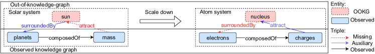
Figure 1. An example of the OOKG entity problem. Our aim is to predict missing facts of the OOKG entities.

Challenge 1: Identifying inter-rule correlations. Previous methods for inductive knowledge embedding mainly focus on modeling one or two hop local neighborhood structures, or mining rules for the OOKG entities. Other complex patterns helpful for the predictions of missing facts, such as inter-rule correlations, are ignored. As shown in Fig. 1, the extracted logic rule $(\mathit{sun},\mathit{surroundedBy},\mathit{planets})$ ${}\land(\mathit{planets},\mathit{composedOf},\mathit{mass})\to(\mathit{sun}$, $\mathit{attract},\mathit{mass})$ describes the principle of the solar system. Given the fact that the solar system, and atom system are correlated (since the “nucleus” is the scale-down “sun” in the atom), the missing fact $(\mathit{nucleus},\mathit{Surround}$- $\mathit{edBy},\mathit{electrons})$ and new rule $(\mathit{nucleus},\mathit{surroundedBy},\mathit{electrons})\land(\mathit{electrons},\mathit{composedOf},\mathit{charges})\to(\mathit{nucleus},\mathit{attract},\mathit{charges})$ are obtained easily through the analogy between the solar and atom system. In this work, such correlations are extracted and modeled to facilitate inductive KGE methods. By identifying inter-rule correlations, our proposed method is able to discover most (more than 80%) of symmetric path (SP) rules used by VN network (He et al., 2020) and other useful patterns in knowledge graphs (KGs) to further improve embedding learning (see §4.1.3).

Challenge 2: Capturing the interactions among rule mining, rule inference, and embedding. LAN (Wang et al., 2019a) utilizes constant logic rule confidences to measure neighboring relations’ usefulness, while VN network (He et al., 2020) employs the heuristic rule mining method (i.e., AMIE+ (Galárraga et al., 2015)). In that case, prior work fails to capture interactions among rule mining, rule inference, and embedding. In fact, these three processes (i.e., rule mining, rule inference, and embedding) benefit and complement each other. Specifically, rules can infer missing facts more accurately with refined embeddings, while predicted facts help to learn the embeddings of higher quality (Guo et al., 2018). Besides, rule learning using KG embeddings can transform the mining process from discrete graph search into calculations in continuous spaces, reducing the search space remarkably (Zhang et al., 2019a). In this work, we design an iterative framework for rule mining, rule inference, and embedding to incorporate the relations among the above three stages, as Fig. 2 illustrates.

To address the two challenges listed above, we propose an inductive knowledge embedding framework, named virtual neighbor network with inter-rule correlations (VNC), to iteratively infer virtual neighbors for the OOKG entities with logic rules and inter-rule correlations. As Fig. 2 illustrates, VNC is composed of three main stages: (i) rule mining, (ii) rule inference, and (iii) embedding. In the rule mining process, to capture useful complex patterns in KG, both logic rules and inter-rule correlations are extracted from KGs, and assigned confidence scores via calculations over relation embeddings. To alleviate the data sparsity problem, virtual neighbors (VNs) of entities are inferred utilizing the deductive capability of rules. By solving a convex rule-constrained problem, soft labels of virtual neighbors are optimized. Next, the KG with softly predicted VNs is input to the GNN-based encoder, which consists of structure-aware and query-aware layers. Moreover, entity embeddings obtained by aggregating neighbors in the encoder are taken as the initialization for the embedding-based decoder. Finally, optimal entity and relation embeddings are derived by minimizing the global loss over observed and softly labeled fact triples. The above three processes are conducted iteratively during training.

Our contributions can be summarized as follows: (i) We propose an inductive knowledge embedding paradigm, named VNC, to address the OOKG entity problem. (ii) We develop an embedding-enhanced rule mining scheme to identify logic rules and inter-rule correlations simultaneously. (iii) We design an iterative framework to explore the interactions among rule mining, rule inference, and embedding. (iv) Experimental results show that the proposed VNC achieves state-of-the-art performance in both link prediction and triple classification tasks.

2. Related Work

Knowledge graph completion. Knowledge graph completion (KGC) methods have been extensively studied and mainly fall under the embedding-based paradigm (Teru et al., 2020; Wang et al., 2021). The aim of knowledge graph embedding (KGE) methods is to map the entities and relations into continuous vector spaces and then measure the plausibility of fact triples using score functions. Early work designs shallow models solely relying on triples in the observed KGs (Bordes et al., 2011, 2013; Nickel et al., 2011). One line of recent works focus on devising more sophisticated triple scoring functions, including TransH (Wang et al., 2014), TransR (Lin et al., 2015b), RotatE (Sun et al., 2019), DistMult (Yang et al., 2015), and Analogy (Liu et al., 2017). Another line of recent methods is to incorporate useful information beyond triples, including relation paths (Neelakantan et al., 2015; Zhang et al., 2018) and logic rules (Guo et al., 2018; Ding et al., 2018; Niu et al., 2020; Zhang et al., 2019a). Besides, deep neural network based methods (Dettmers et al., 2018; Wang et al., 2019c, [n. d.]) and language model based methods (Wang et al., 2021, 2022) also show promising performance.

Inductive knowledge embedding. Despite the success in KGC problem, the above KGE methods still focus on the transductive settings, requiring all the test entities to be seen during training. Motivated by the limitations of traditional KGE methods, recent works (Hamaguchi et al., 2017; Wang et al., 2019a; Dai et al., 2021; Baek et al., 2020) take the known neighbors of the emerging entities as the inputs of inductive models. Hamaguchi et al. (2017) employ the graph neural network (GNN) and aggregate the pretrained representations of the existing neighbors for unseen entities. To exploit information of redundancy and query relations in the neighborhood, LAN (Wang et al., 2019a) utilizes a logic attention network as the aggregator. GEN (Baek et al., 2020) and HRFN (Zhang et al., 2021) design meta-learning frameworks for GNNs to simulate the unseen entities during meta-training. However, they utilize unseen-to-unseen triples, which are unavailable in the OOKG entity problem. VN network (He et al., 2020) alleviates the data sparsity problem by inferring virtual neighbors for the OOKG entities. In addition, InvTransE and InvRotatE (Dai et al., 2021) represent OOKG entities with the optimal estimations of translational assumptions. Another type of inductive methods represent unseen entities via learning entity-independent semantics, including rule based (Sadeghian et al., 2019) and GNN based (Teru et al., 2020; Chen et al., 2021) methods. However, the above methods focus on a different inductive KGC task (i.e., completing an entirely new KG during testing), and are not able to take advantage of embeddings of known entities or inter-rule correlations. In our experiments, we also conduct a comprehensive comparison between our proposed model and entity-independent methods (see §6.3).

The most closely related work is MEAN (Hamaguchi et al., 2017), LAN (Wang et al., 2019a), VN network (He et al., 2020), InvTransE and InvRotatE (Dai et al., 2021). These previous inductive embedding methods ignore inter-rule correlations, and do not capture interactions among rule mining, rule inference, and embedding. In our proposed model VNC, to model useful complex patterns in graphs, logic rules and inter-rule correlations are identified simultaneously. We design an iterative framework to incorporate interactions among rule mining, rule inference, and embedding.

3. Definitions

Definition 3.0 (Knowledge graph).

A knowledge graph $\mathcal{K}$ can be regarded as a multi-relational graph, consisting of a set of observed fact triples, i.e., $\mathcal{O}=\{t_{o}\}$, where $t_{o}=(e_{i},r_{k},e_{j})$. Each fact triple consists of two entities $e_{i},e_{j}\in\mathcal{E}_{o}$, and one type of relation $r_{k}\in\mathcal{R}$, where $\mathcal{E}_{o}$ and $\mathcal{R}$ are the entity and relation sets respectively. For each triple $(e_{i},r_{k},e_{j})\in\mathcal{K}$, we denote the reverse version of relation $r_{k}$ as $r^{-1}_{k}$ and add $(e_{j},r^{-1}_{k},e_{i})$ to the original KG $\mathcal{K}$.

Definition 3.0 (Out-of-knowledge-graph entity problem).

Following (Hamaguchi et al., 2017; Dai et al., 2021), we formulate the out-of-knowledge-graph (OOKG) entity problem as follows. The auxiliary triple set $\mathcal{AUX}$ contains the unseen entities $\mathcal{E}_{u}=\mathcal{E}_{aux}/\mathcal{E}_{o}$, and each triple in $\mathcal{AUX}$ contains exactly one OOKG entity and one observed entity. And $\mathcal{O}$ is observed during training, while the auxiliary triple set $\mathcal{AUX}$ connecting OOKG and observed entities is only accessible at test time. Note that, no additional relations are involved in $\mathcal{AUX}$. Given $\mathcal{AUX}$ and $\mathcal{O}$, the goal is to correctly identify missing fact triples that involve the OOKG entities.

Definition 3.0 (Logic rules).

For logic rules, following (Guo et al., 2018; Ding et al., 2018), we consider a set of first-order logic rules with different confidence values for a give KG, represented as $\mathcal{F}^{\mathit{logic}}=\{(f^{\mathit{logic}}_{m},\lambda^{\mathit{logic}}_{m})\}_{m=1}^{M}$, where $f^{\mathit{logic}}_{m}$ is the $m$-th logic rule. $\lambda^{\mathit{logic}}_{m}\in[0,1]$ denotes its confidence value, and rules with higher confidence values are more likely to hold. Here, $f^{\mathit{logic}}_{m}$ is in the form of $\mathit{body}\rightarrow\mathit{head}$. In this paper, we restrict rules to be Horn clause rules, where the rule head is a single atom, and the rule body is a conjunction of one or more atoms. For example, such kind of logic rule can be:

(1) $$(x,\mathit{surroundedBy},y)\land(y,\mathit{composedOf},z)\rightarrow(x,\mathit{attract},z),$$

where $x$, $y$, $z$ are entity variables. Similar to previous rule learning work (Guo et al., 2018; Galárraga et al., 2013), we focus on closed-path (CP) rules to balance the expressive power of mined rules and the efficiency of rule mining. In a CP rule, the sequence of triples in the rule body forms a path from the head entity variable to the tail entity variable of the rule head. By replacing all variables with concrete entities in the given KG, we obtain a grounding of the rule. For logic rule $f^{\mathit{logic}}_{m}$, we denote the set of its groundings as $\mathcal{G}_{m}^{\mathit{logic}}=\{g^{\mathit{logic}}_{mn}\}_{n=1}^{N_{m}}$.

Definition 3.0 (Inter-rule correlations).

In addition to logic rules, we also consider a set of inter-rule correlations with different confidence levels, denoted as $\mathcal{F}^{\mathit{corr}}=\{(f^{\mathit{corr}}_{v},\lambda^{\mathit{corr}}_{v})\}_{v=1}^{V}$, where $f^{\mathit{corr}}_{v}$ is the $v$-th inter-rule correlation and $\lambda^{\mathit{corr}}_{v}$ is the corresponding confidence value. Based on the logic rule $f^{\mathit{logic}}_{m}$, we define the corresponding inter-rule correlations as:

(2) $$f^{\mathit{corr}}_{v_{\mathit{mpq}}}:f^{\mathit{logic}}_{m}\xrightarrow{\mathit{path}_{q}\left(f^{\mathit{logic}}_{m},f^{\prime\mathit{logic}}_{\mathit{mp}}\right)}f^{\prime\mathit{logic}}_{\mathit{mp}},$$

where $f^{\prime logic}_{mp}$ is the $p$-th “incomplete” logic rule in the same form as $f^{logic}_{m}$ but with one missing triple in the rule body. For example, as Fig. 1 shows, the rule for the atom system are incomplete since $(x,\mathit{surroundedBy},y)$ in the logic rule $(x,\mathit{surroundedBy},y)\land(y,\mathit{composedOf},z)\rightarrow(x,\mathit{attract},z)$ is missing. Note that the rules with only rule head missing are not regarded as the “incomplete” rules, because the missing rule head can be directly inferred by extracted logic rules. The $q$-th inter-rule path between the logic rule $f^{\mathit{logic}}_{m}$ and incomplete rule $f^{\prime\mathit{logic}}_{\mathit{mp}}$ is represented as follows: $\small\mathit{path}_{q}(f^{\mathit{logic}}_{m},f^{\prime}{{}^{\mathit{logic}}}_{\mathit{mp}}):(x_{1},r_{1},x_{2})\land{}(x_{2},r_{2},x_{3})\land{}\cdots\land(x_{k},r_{k},x_{k+1}),$ where $r_{i}\in\mathcal{R}$ denotes a relation in KG and $x_{i}$ is the entity variable. To represent the correlations between rules, we assume that the inter-rule path only exists between entities of the same position in two rules. For example, in Fig. 1, the inter-rule path is $(\mathit{sun},\mathit{scaleDown},\mathit{nucleus})$ indicating that the nucleus is the scaled-down sun in the atom system. Similar to the logic rules, we obtain the set of groundings $\mathcal{G}^{\mathit{corr}}_{v}=\{g^{\mathit{corr}}_{\mathit{vw}}\}_{w=1}^{W_{v}}$ for $f^{\mathit{corr}}_{v}$ by replacing variables with concrete entities.

Definition 3.0 (Virtual neighbors).

To address the data sparsity problem, we introduce virtual neighbors into the original KG. As mentioned above, virtual neighbors are inferred by the extracted rules (i.e., logic rules and inter-rule correlations). Specifically, if a triple $(e^{\prime}_{i},r^{\prime}_{k},e^{\prime}_{j})$ inferred by rules does not exist in either the observed triple set $\mathcal{O}$ or auxiliary triple set $\mathcal{AUX}$, we suppose that $e^{\prime}_{i}$ and $e^{\prime}_{j}$ are the virtual neighbors to each other. In our paper, we denote the set containing such kind of triples as $\mathcal{VN}=\{t_{vn}\}$, where $t_{vn}$ is a triple with the virtual neighbors.

4. Method

In this section, we describe the VNC framework, our proposed method for the OOKG entity problem. As illustrated in Fig. 2, the framework has three stages: rule mining (§4.1), rule inference (§4.2), and embedding (§4.3). In the rule mining stage, Given the knowledge graph, the rule pool is first generated by searching plausible paths, and confidence values are calculated using the current relation embeddings $\mathbf{R}$. Then, in the rule inference stage, a new triple set with virtual neighbors $\mathcal{VN}=\{t_{\mathit{vn}}\}$ is inferred from rule groundings. And each predicted triple $t_{\mathit{vn}}$ is assgined a soft label $s(t_{\mathit{vn}})\in[0,1]$ by solving a rule-constrained optimization problem. The knowledge graph with virtual neighbors is inputted into GNN-based encoder consisting of both structure and query aware layers. Next, with the entity embeddings $\mathbf{E}=\mathbf{H}^{O}$, where $\mathbf{H}^{O}$ is the output of GNN layers, the embedding-based decoder projects relations into embeddings $\mathbf{R}$ and calculate the truth level $\phi(\cdot)$ for each fact triple as follows (take DistMult (Yang et al., 2015) as an example):

(3) $$\phi(e_{i},r_{k},e_{j})=\mathbf{e}_{i}^{T}\mathbf{R}_{k}\mathbf{e}_{j},$$

where $\mathbf{e}_{i},\mathbf{e}_{j}$ are the normalized entity embeddings for entity $e_{i}$ and $e_{j}$ respectively, and $\mathbf{R}_{k}$ is a diagonal matrix for relation $r_{k}$. These three stages are conducted iteratively during training (see §4.4).

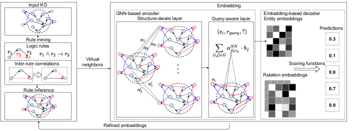
Figure 2. An overview of VNC. VNC has three main stages: rule mining, rule inference, and embedding.

4.1. Rule mining

Given the observed knowledge graph, rule mining stage first generates a pool of logic rules by finding possible paths. Then, based on the complete logic rules, inter-rule correlations are discovered by searching incomplete rules and inter-rule paths. Finally, the confidence values are computed using relation embeddings.

4.1.1. Rule pool generation

Before computing confidence scores, rules should be extracted from the observed KG.

For logic rules, we are only interested in closed-path (CP) rules. Therefore, given the rule head, the search for candidate logic rules is reduced to finding plausible paths for rule bodies. Specifically, one of fact triples in the observed KG $\mathcal{K}$ (e.g., $(e_{1},r,e_{2})\in\mathcal{O}$) is first taken as the candidate rule head, and then the possible paths between the head entity and tail entity of the rule head (e.g., $(e_{1},r_{1},e_{3})\land(e_{3},r_{2},e_{2})$) is extracted. In this way, the candidate logic rule $(x,r_{1},z)\land(z,r_{2},y)\rightarrow(x,r,y)$ is induced from the given KG. For computational efficiency, we restrict the length of paths in rule bodies to at most 2 (i.e., the length of rules is restricted to at most 3). Note that, there may still exist numerous redundant and low quality rules in the above extraction process. Therefore, following (Galárraga et al., 2013; Zhang et al., 2019a), further filtering is conducted, and only rules with $\mathit{support}>1$, $\mathit{head}\ \mathit{coverage}>\alpha_{HC}$, and $\mathit{standard}\ \mathit{confidence}>\alpha_{SC}$ are selected, where $\alpha_{HC}$ and $\alpha_{SC}$ are preset thresholds.

Based on mined logic rules, there are two steps for generating possible inter-rule correlations: (i) Finding incomplete rules. To this end, our aim is to identify all the “incomplete” rules for the mined logic rules. Specifically, given the $m$-th logic rule $f^{\mathit{logic}}_{m}$ in $\mathcal{K}$, a set of “incomplete” logic rules $\{f^{\prime\mathit{logic}}_{mp}\}$ in the same form as $f^{\mathit{logic}}_{m}$ but with one missing triple in the rule body is recognized in this step. For example, for the logic rule of length 2 (e.g., $(x,r_{1},y)\rightarrow(x,r,y)$), there exists only one “incomplete” logic rule (e.g., $(x,r_{1},y)\rightarrow(x,r,y)$ with $(x,r_{1},y)$ missing). (ii) Searching plausible inter-rule paths. To extract inter-rule paths, we first obtain groundings of logic rules and “incomplete” rules by replacing variables with concrete entities. For example, a grounding of logic rule $(x,r_{1},z)\land(z,r_{2},y)\rightarrow(x,r,y)$ can be $(e_{1},r_{1},e_{2})\land(e_{2},r_{2},e_{3})$ $\rightarrow(e_{1},r,e_{3})$, and a grounding of the corresponding “incomplete” rules can be $(e^{\prime}_{1},r_{1},e^{\prime}_{2})\land(e^{\prime}_{2},r_{2},e^{\prime}_{3})\rightarrow(e^{\prime}_{1},r,e^{\prime}_{3})$, where $e_{i},\ e^{\prime}_{i}\in\mathcal{E}_{o}$ and $(e^{\prime}_{1},r_{1},e^{\prime}_{2})\notin\mathcal{O}$. Then, the paths between entities of the same position in logic and “incomplete” rules (e.g., paths between $e_{1}$ and $e^{\prime}_{1}$) are searched. Here, we estimate the reliability of inter-rule paths using the path-constraint resource allocation (PCRA) algorithm (Lin et al., 2015a), and keep paths with $\mathit{Reliability}>\alpha_{PCRA}$, where $\alpha_{PCRA}$ is the threshold for the path reliability. For computational efficiency, the length of inter-rule paths is limited to at most 3. In the next step, similar to mining logic rules, we filter out inter-rule correlations of low quality with $\mathit{support}$, $\mathit{head}\ \mathit{coverage}$, and $\mathit{standard}\ \mathit{confidence}$.

4.1.2. Confidence computation

Given the generated rule pool and current relation embedding $\mathbf{R}$, the confidence computation assigns a score $\lambda_{m}$ for each extracted rule $f_{m}$.

For each logic rule, the rule body and rule head can be considered as two associated paths. Inspiring by previous works (Zhang et al., 2019a; Omran et al., 2018), the confidence level of each logic rule can be measured by the similarity between paths of the rule body and rule head. To be specific, suppose the path of the rule body $\mathit{path}_{\mathit{body}}:(x_{1},r_{1},x_{2})\land(x_{2},r_{2},x_{3})\land\cdots\land(x_{k},r_{k},x_{k+1})$, and the path of the rule head $\mathit{path}_{\mathit{head}}:(x_{1},r,x_{k+1})$, the corresponding confidence level $\lambda^{logic}_{m}$ is calculated as follows:

(4) $$\lambda^{\mathit{logic}}_{m}={\rm sim}(\mathbf{path}_{\mathit{body}},\mathbf{path}_{\mathit{head}}),$$

where $\mathbf{path}_{\mathit{body}}$ and $\mathbf{path}_{\mathit{head}}$ are embeddings for the paths of the rule body and rule head, respectively. And ${\rm sim}(\cdot)$ is the similarity function. In VNC, we consider a variety of methods based on translating or bilinear operations in the embedding stage. Thus, we define two kinds of similarity functions and path representations for different embedding methods. For translational decoders (e.g., TransE), the path representations and similarity function in Eq. 4 are defined as follows:

(5) $$\begin{split}\mathbf{path}_{\mathit{body}}&=\mathbf{r}_{1}+\mathbf{r}_{2}+\cdots+\mathbf{r}_{k},\ \mathbf{path}_{\mathit{head}}=\mathbf{r},\\ \lambda^{\mathit{logic}}_{m}&=||\mathbf{path}_{\mathit{body}}-\mathbf{path}_{\mathit{head}}||_{2},\\ \end{split}$$

where $\mathbf{r}_{i}$ and $\mathbf{r}$ are vector embeddings for relation $r_{i}$ and $r$, and similarity function is defined by the $L_{2}$-norm. For bilinear decoders (e.g., DistMult), the path representations and similarity function in Eq. 4 are defined as follows:

(6) $$\begin{split}\mathbf{path}_{\mathit{body}}&=\mathbf{M}_{r_{1}}+\mathbf{M}_{r_{2}}+\cdots+\mathbf{M}_{r_{k}},\\ \mathbf{path}_{\mathit{head}}&=\mathbf{M}_{r},\\ \lambda^{logic}_{m}&=||\mathbf{path}_{\mathit{body}}-\mathbf{path}_{\mathit{head}}||_{F},\\ \end{split}$$

where $\mathbf{M}_{r_{i}}$ and $\mathbf{M}_{r}$ are matrix embeddings for relation $r_{i}$ and $r$, and similarity function is defined by the Frobenius norm.

On this basis, we calculate confidence scores of inter-rule correlations. Specifically, for inter-rule correlation in Eq. 2, we consider the confidences of logic rule and “incomplete” rule simultaneously, and define the confidence level $\lambda^{\mathit{corr}}_{v_{\mathit{mpq}}}$ for inter-rule correlation $f^{\mathit{corr}}_{v_{\mathit{mpq}}}$ as follows:

(7) $$\lambda^{\mathit{corr}}_{v_{\mathit{mpq}}}=\lambda^{\mathit{logic}}_{m}\cdot\lambda^{\prime\mathit{logic}}_{\mathit{mp}},$$

where $\lambda^{\mathit{logic}}_{m}$ and $\lambda^{\prime\mathit{logic}}_{mp}$ are the confidences of logic rule $f^{\mathit{logic}}_{m}$ and “incomplete” rule $f^{\prime\mathit{logic}}_{mp}$, respectively. The confidence $\lambda^{\prime\mathit{logic}}_{mp}$ of “incomplete” rule $f^{\prime\mathit{logic}}_{mp}$ is regarded as the probability of inferring the missing triple using the observed path (from the head entity to the tail entity of the missing triple). For example, the confidence $\lambda^{\prime\mathit{logic}}_{mp}$ for “incomplete” rule $f^{\prime\mathit{logic}}_{mp}:(x_{1},r_{1},x_{2})\land(x_{2},r_{2},x_{3})\rightarrow(x_{1},r,x_{3})$ (with $(x_{1},r_{1},x_{2})$ missing) is computed as (for bilinear decoders): $\lambda^{\prime\mathit{logic}}_{mp}=\|\mathbf{M}_{r}+\mathbf{M}_{r^{-1}_{2}}-\mathbf{M}_{r_{1}}\|_{F},$ where $\mathbf{M}_{r^{-1}_{i}}$ is the matrix embedding for the reverse version of the relation $r_{i}$. Since unreliable paths are filtered out during rule pool generation, the reliability of inter-rule path is not considered.

4.1.3. Discussion: relation to symmetric path rules

In VN network (He et al., 2020), to capture long-distance semantic similarities between entities, symmetric path (SP) rules in KGs are identified. In fact, many symmetric path rules can be transformed into inter-rule correlations. For example, the SP rule shown in Fig. 3(a) can be represented by the inter-rule correlation in Fig. 3(b), since symmetric paths in the rule body and head share several entities and relations. Motivated by this, as Fig. 3(c) and 3(d) shows, we count the number of the shared rules (blue bars) used by VN network and VNC on FB15K Subject 20 and WN18 Subject 20. The results indicate that the VNC framework is capable of extracting most of the symmetric path rules (more than 80%), and identifying abundant graph patterns to further alleviate the data sparsity problem, and improve the embedding quality.

(a) Symmetric path rule.

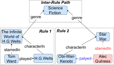
(b) Inter-rule correlation.

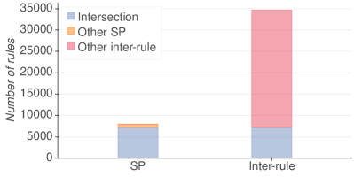
(c) FB15K Subject-20.

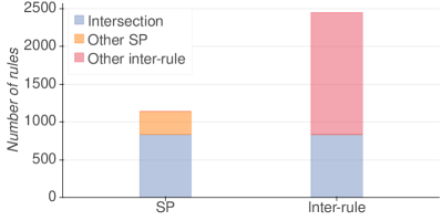
(d) WN18 Subject-20.

Figure 3. (a) and (b) are examples of SP rules and inter-rule correlations, respectively; (c) and (d) demonstrate the intersection between SP rules and inter-rule correlations.

4.2. Rule inference

In the rule inference stage, given the extracted rules, our goal is to infer a new triple set with virtual neighbors $\mathcal{VN}$ and assign a soft label $s(t_{vn})$ to each predicted triple $t_{vn}\in\mathcal{VN}$.

4.2.1. Rule modeling

To predict a new triple $t_{vn}\in\mathcal{VN}$, we replace variables in extracted rules with concrete entities to obtain rule groundings. To model rule groundings, we adopt t-norm based fuzzy logics (Hájek, 1998). The key idea here is to compute the truth level of a grounding rule using the truth levels of its constituent triples and logical connectives (e.g., $\land$ and $\rightarrow$). Following (Guo et al., 2018; Hájek, 1998), logical connectives associated with the logical conjunction ($\land$), disjunction($\lor$), and negation ($\neg$) are defined as follows:

(8) $$\small\begin{split}I(a\land b)&=I(a)\cdot I(b),\\ I(a\lor b)&=I(a)+I(b)-I(a)\cdot I(b),\\ I(\neg a)&=1-I(a),\end{split}$$

where $a$ and $b$ denote logical expressions, which can be the atom triple or multiple triples combined by logical connectives. $I(\cdot)$ is the truth level function. If $a=(e_{1},r_{1},e_{2})$ is a single triple, $I(a)$ is defined by Eq. 3, i.e., $I(a)=\phi(e_{1},r_{1},e_{2})$. For combined multiple triples, we can calculate the truth value using Eq. 8 recursively. For example, for a rule grounding $a\rightarrow b$, the truth value can be computed as: $I(a\rightarrow b)=I(\neg a\lor b)=I(a)\cdot I(b)-I(a)+1$.

4.2.2. Soft label prediction

In this stage, our goal is to assign a soft label $s(x_{vn})\in[0,1]$ for each triple $t_{vn}\in\mathcal{VN}$, using the current KG embeddings (i.e., $\mathbf{E}$ and $\mathbf{R}$) and rule groundings (i.e., $\mathcal{G}^{logic}$ and $\mathcal{G}^{corr}$). To this end, we establish and solve a rule-constrained optimization problem. Here, the optimal soft label $s(t_{\mathit{vn}})$ should keep close to truth level $I(t_{\mathit{vn}})$, while constrained by the rule groundings. For the first characteristic, we minimize a square loss over the soft label $s(t_{vn})$ and truth level $I(t_{\mathit{vn}})$. For the second characteristic, we impose rule constraints on the predicted soft labels $\mathcal{S}=\{s(t_{\mathit{vn}})\}$. To be specific, given a rule $f_{m}$ and soft labels $\mathcal{S}$, rule groundings $g_{\mathit{mn}}$ is expected to be true, i.e., $I(g_{\mathit{mn}}|\mathcal{S})=1$ with confidence $\lambda_{m}$. Here, the conditional truth level $I(g_{mn}|\mathcal{S})$ can be calculated recursively using the logical connectives in Eq. 8. Specifically, for each logic rule grounding $g^{\mathit{logic}}_{mn}:(e_{i},r_{b},e_{j})\rightarrow(e_{i},r_{h},e_{j})$, where $(e_{i},r_{b},e_{j})\in\mathcal{O}$ and $(e_{i},r_{h},e_{j})\in\mathcal{VN}$, the conditional truth level $I(g^{\mathit{logic}}_{mn}|\mathcal{S})$ is calculated as: $I(g^{\mathit{logic}}_{mn}|\mathcal{S})=I(e_{i},r_{b},e_{j})\cdot s(e_{i},r_{h},e_{j})-I(e_{i},r_{b},e_{j})+1,$ where $I(e_{i},r_{b},e_{j})$ is the truth level defined in Eq. 3 computed using the current embedding, while $s(e_{i},r_{h},e_{j})$ is a soft label to infer. Similarly, for each grounding of inter-rule correlations $g^{corr}_{vw}:g^{\mathit{logic}}_{b}\rightarrow g^{\prime}{{}^{\mathit{logic}}}_{h}$, where $g^{logic}_{b}$ is a logic rule grounding and $g^{\prime}{{}^{\mathit{logic}}}_{h}$ is a grounding for the corresponding “incomplete” logic rule, the conditional truth level $I(g^{\mathit{corr}}_{vw}|\mathcal{S})$ can be computed as:

(9) $$I(g^{\mathit{corr}}_{vw}|\mathcal{S})=I(g^{\mathit{logic}}_{b})\cdot I(g^{\prime\mathit{logic}}_{h}|\mathcal{S})-I(g^{\mathit{logic}}_{b})+1,$$

where $I(g^{\mathit{logic}}_{b})$ is the truth level for the logic rule grounding $g^{\mathit{logic}}_{b}$, and $I(g^{\prime logic}_{h}|\mathcal{S})$ denotes the conditional truth level for the “incomplete” logic rule grounding $g^{\prime\mathit{logic}}_{h}$. Since triples in $g^{\mathit{logic}}_{b}$ are observed in KG, we suppose $I(g^{\mathit{logic}}_{b})=1$ for simplicity. Similar to Eq. 4.2.2, the conditional truth level $I(g^{\prime\mathit{logic}}_{h}|\mathcal{S})$ can be computed recursively according to logical connectives.

Combining two characteristics, we introduce the slack variables $\xi^{\mathit{logic}}_{mn}$ and $\xi^{\mathit{corr}}_{\mathit{vws}}$, and establish the following optimization problem to obtain the optimal soft labels:

(10) $$\small\begin{split}\min_{S,\xi}&{\frac{1}{2}\cdot\sum_{t_{vn}\in\mathcal{VN}}{(s(t_{vn})-I(t_{vn}))^{2}}}+C\cdot\left(\sum_{m,n}{\xi^{\mathit{logic}}_{mn}}+\sum_{v,w}{\xi^{\mathit{corr}}_{vw}}\right)\mbox{}\\ &\text{such that }\lambda^{\mathit{logic}}_{m}(1-I(g^{\mathit{logic}}_{mn}|S))\leq\xi^{\mathit{logic}}_{mn}\\ &\phantom{\text{such that }}\lambda^{\mathit{corr}}_{v}(1-I(g^{\mathit{corr}}_{vw}|S))\leq\xi^{\mathit{corr}}_{vw}\\ &\phantom{\text{such that }}\xi^{\mathit{logic}}_{mn}\geq 0,\xi^{\mathit{corr}}_{vw}\geq 0,0\leq s(t_{vn})\leq 1,\end{split}$$

where $C$ is the constant penalty parameter, and $\lambda^{\mathit{logic}}_{m}$ and $\lambda^{\mathit{corr}}_{v}$ are the confidence values for logic rule $f^{\mathit{logic}}_{m}$ and inter-rule correlation $f^{\mathit{corr}}_{v}$ respectively. Note that, for the optimization problem in Eq. 10, all the constraints are linear functions w.r.t $s(t_{\mathit{vn}})$, and this kind of the optimization problem is convex (Guo et al., 2018). Therefore, we can obtain the closed-form solution for this problem:

(11) $$\small\begin{split}s(t_{vn})=&\left[I(t_{\mathit{vn}})+C\cdot\left(\sum_{m,n}{\lambda^{\mathit{logic}}_{m}\nabla_{s(t_{\mathit{vn}})}{I(g^{\mathit{logic}}_{mn}|S)}}\right.\right.\\ &\,\,\,\left.\left.+\sum_{v,w}{\lambda^{\mathit{corr}}_{v}\nabla_{s(t_{\mathit{vn}})}{I(g^{\mathit{corr}}_{vw}|S)}}\right)\right]_{0}^{1},\\ \end{split}$$

where $\nabla_{s(t_{\mathit{vn}})}{I(g^{\mathit{logic}}_{mn}|S)}$ and $\nabla_{s(t_{\mathit{vn}})}{I(g^{\mathit{corr}}_{vw}|S)}$ denote the gradients of $I(g^{\mathit{logic}}_{mn}|S)$ and $I(g^{\mathit{corr}}_{vw}|S)$ w.r.t $s(t_{\mathit{vn}})$ respectively, which are both constants. $[\cdot]_{0}^{1}=\min(\max(x,0),1)$ is a truncation function.

4.3. Embedding

In the embedding stage, the knowledge graph with softly labeled virtual neighbors is inputted into the GNN-based encoder and embedding-based decoder. In this way, entities and relations in KG are projected into embeddings $\mathbf{E}$ and $\mathbf{R}$.

4.3.1. GNN-based encoder

Similar to previous works (Wang et al., 2019a; He et al., 2020), our encoder consists of several structure aware layers and one query aware layer. To model connectivity structures of the given KG, we adopt weighted graph convolutional network (WGCN) (Shang et al., 2019) as the structure aware layers. In each layer, different relation types are assigned distinct attention weights. The $l$-th structure aware layer can be formulated as follows:

(12) $$\small\begin{split}\mathbf{a}_{i}^{(l)}&=\mathbf{W}^{(l)}\cdot\left(\sum_{(e_{i},r,e_{j})\in\mathcal{O}\cup\mathcal{VN}}{\alpha_{r}^{(l)}\mathbf{h}^{(l-1)}_{j}}\right),\\ \mathbf{h}_{i}^{(l)}&=\tanh\left(\mathbf{a}_{i}^{(l)}+\mathbf{h}_{i}^{(l-1)}\mathbf{W}^{(l)}\right),\end{split}$$

where $\alpha_{r}$ are the attention weights for relation $r$. $\mathbf{h}_{i}^{(l)}$ is the embedding of entity $e_{i}$ at the $l$ th layer. $\mathbf{W}^{(l)}$ is the connection matrix for the $l$ th layer. Here, we randomly initialize the input entity embedding $\mathbf{h}^{(0)}_{i}$ during training. Besides the structure information, given the query relation in each inputted triple, an ideal aggregator is able to focus on the relevant facts in the neighborhood. To this end, the importances of neighbors are calculated based on the neural network mechanism (Wang et al., 2019a). Specifically, given a query relation $r_{q}\in\mathcal{R}$, the importance of the neighbor $e_{j}$ to entity $e_{i}$ is calculated as: $\alpha^{\rm NN}_{j|i,q}={\rm softmax}(\beta_{j|i,q})=\frac{{\rm exp}(\beta_{j|i,q})}{\sum_{(e_{i},r_{q},e_{j^{\prime}})\in\mathcal{O}\cup\mathcal{VN}}{{\rm exp}(\beta_{j^{\prime}|i,q})}},$ where the unnormalized attention weight $\beta_{j|i,q}$ can be computed as: $\beta_{j|i,q}={\rm LeakyReLU}(\mathbf{u}\cdot[\mathbf{W}_{e}\mathbf{h}_{i};\mathbf{W}_{q}\mathbf{z}_{q};\mathbf{W}_{e}\mathbf{h}_{j}])$, where $\mathbf{u}$, $\mathbf{W}_{e}$, and $\mathbf{W}_{q}$ are the attention parameters, and $\mathbf{z}_{q}$ is the relation-specific parameter for query relation $r_{q}$. ${\rm LeakyReLU}(\cdot)$ is the activation function of the leaky rectified linear unit (Xu et al., 2015). On this basis, we can formulate the query aware layer as follows:

(13) $$\mathbf{h}^{O}_{i}=\sum_{(e_{i},r,e_{j})\in\mathcal{O}\cup\mathcal{VN}}{\alpha^{\rm NN}_{j|i,q}\cdot\mathbf{h}^{I}_{j}},$$

where $\mathbf{h}^{I}_{j}$ is the input embedding for the entity $e_{j}$ from the last structure aware layer. $\mathbf{h}^{O}_{i}$ is the output embedding for the entity $e_{i}$ for the decoder. Note that, in the testing process, we apply the encoder on the auxiliary triples, and initialize the input representation $\mathbf{h}^{(0)}_{i^{\prime}}$ for the OOKG entity $e_{i^{\prime}}$ as the zero vector.

4.3.2. Embedding-based decoder

Given entity embeddings from the GNN-based encoder (i.e., $\mathbf{E}=\mathbf{H}^{O}$, where $\mathbf{H}^{O}$ is the output of the encoder), the decoder aims to learn relation embeddings $\mathbf{R}$, and compute the truth level $\phi(t)$ for each triple $t$. We evaluate various embedding methods in our experiments, including DistMult (Yang et al., 2015), TransE (Bordes et al., 2013), ConvE (Dettmers et al., 2018), and Analogy (Liu et al., 2017) (see §7.2).

4.4. Training algorithm

To refine the current KG embeddings, a global loss over facts with hard and soft labels is utilized in the VNC framework. In this stage, we randomly corrupt the head or tail entity of an observed triple to form a negative triple. In this way, in addition to triples with soft labels $\mathcal{VN}=\{t_{vn}\}$, we collect the observed and negative fact triples with hard labels, i.e., $\mathcal{L}=\{x_{l},y_{l}\}$, where $y_{l}\in\{0,1\}$ is the hard label of the triples. To learn the optimal KG embeddings $\mathbf{E}$ and $\mathbf{R}$, a global loss function over $\mathcal{L}$ and $\mathcal{VN}$ is:

(14) $$\small\min_{\mathbf{E},\mathbf{R}}{\frac{1}{|\mathcal{L}|}\sum_{\mathcal{L}}{l(I(t_{l}),y_{l})}+\frac{1}{|\mathcal{VN}|}\sum_{\mathcal{VN}}{l(I(t_{vn}),s(t_{vn}))}},$$

where we adopt the cross entropy $l(x,y)=-y\log{x}-(1-y)\log{(1-x)}$. $I(\cdot)$ is the truth level function. We use Adam (Kingma and Ba, 2015) to minimize the global loss function. In this case, the resultant KG embeddings fit the observed facts while constrained by rules. Algorithm 1 summarizes the training process of VNC. Before training, rule pools are generated by finding plausible paths, and rules of low quality are filtered out (line 1). In each training step, we compute rules $\lambda^{\mathit{logic}}$ and $\lambda^{\mathit{corr}}$ using current relation embeddings to form rule sets $\mathcal{F}^{\mathit{logic}}$ and $\mathcal{F}^{\mathit{corr}}$ (line 3). Then, in the rule inference stage, we infer new triples $\mathcal{VN}=\{t_{\mathit{vn}}\}$ using rule groundings, and assign a soft label $s{t_{\mathit{vn}}}$ to each predicted fact triples by solving a rule constrained optimization problem (line 4-6). Next, the knowledge graph with virtual neighbors is inputted into the GNN-based encoder and embedding-based decoder. In this way, relations and entities are mapped into embeddings (line 7). Finally, the overall loss over fact triples with hard and soft labels is obtained (line 8-9), and embeddings as well as model parameters are updated (line 10).

Algorithm 1 Training algorithm of VNC.

1:Triples with hard labels $\mathcal{L}$; randomly initialized entity and relation embeddings $\mathbf{E}$ and $\mathbf{R}$; parameters $\mathbf{\Theta}$ for encoder and decoder.

2:The extracted rule set $\mathcal{F}^{\mathit{logic}}$ and $\mathcal{F}^{\mathit{corr}}$; trained encoder and decoder; optimal embeddings $\mathbf{E}$ and $\mathbf{R}$;

3:Generate rule pools, and filter out rules of low quality;

4:while Training process not terminated do

5:    Compute rule confidences $\lambda^{\mathit{logic}}$ and $\lambda^{\mathit{corr}}$, and form rule sets $\mathcal{F}^{\mathit{logic}}$ and $\mathcal{F}^{\mathit{corr}}$ (Eq. 4 and 7);

6:    Find rule groundings $\mathcal{G}^{\mathit{logic}}$ and $\mathcal{G}^{\mathit{corr}}$;

7:    Infer $\mathcal{VN}=\{t_{\mathit{vn}}\}$ and compute the truth level $I(t_{\mathit{vn}})$ for each triple $t_{\mathit{vn}}$ (Eq. 3);

8:    Calculate the conditional truth level $I(g|\mathcal{S})$ (Eq. 9);

9:    Obtain the optimal soft labels $\mathcal{S}=\{s(t_{\mathit{vn}})\}$ (Eq. 10 and 11);

10:    Obtain embeddings $\mathbf{E}$ and $\mathbf{R}$ (Eq. 3,  12, and  13);

11:    Compute the global loss over $\mathcal{L}$ and $\mathcal{VN}$ (Eq. 14);

12:    Update $\mathbf{E}$, $\mathbf{R}$ and $\mathbf{\Theta}$;

13:end while

5. Experiments

Research questions. We aim to answer the following research questions: (RQ1) Does VNC outperform state-of-the-art methods on the OOKG entity problem? (See §6.1–§6.3.) (RQ2) How do the inter-rule correlations and iterative framework contribute to the performance? (See §7.1.) (RQ3) What is the influence of the decoder, embedding dimension, and penalty parameter on the performance? (See §7.2.) (RQ4) Is VNC able to identify useful inter-rule correlations in the knowledge graph? (See §7.3.)

Datasets. We evaluate VNC on three widely used datasets: YAGO37 (Guo et al., 2018), FB15K (Bordes et al., 2013), and WN11 (Socher et al., 2013). For link prediction, we use three benchmark datasets: YAGO37 and FB15K. We create Subject-R and Object-R from each benchmark dataset, varying OOKG entities’ proportion ($R$) as 5%, 10%, 15%, 20%, and 25% following (Wang et al., 2019a). For triple classification, we directly use the datasets released in (Hamaguchi et al., 2017) based on WN11, including Head-$N$, Tail-$N$ and Both-$N$, where $N=\{1000,3000,5000\}$ testing triples are randomly sampled to construct new datasets. Tab. 1 gives detailed statistics of the datasets.

Baselines. We compare the performance of VNC against the following baselines: (i) MEAN(Hamaguchi et al., 2017)utilizes the graph neural network (GNN) and generates embeddings of OOKG entities with simple pooling functions. (ii) LSTM(Wang et al., 2019a)is a simple extension of MEAN, where the LSTM network (Hamilton et al., 2017) is used due to its large expressive capability. (iii) LAN(Wang et al., 2019a)uses a logic attention network as the aggregator to capture information of redundancy and query relations in the neighborhood. (iv) GEN(Baek et al., 2020)develops a meta-learning framewrok to simulate the unseen entities during meta-training. (v) VN network(He et al., 2020)infers additional virtual neighbors for OOKG entities to alleviate the data sparsity problem. (vi) InvTransEand InvRotatE (Dai et al., 2021) obtain optimal estimations of OOKG entity embeddings with translational assumptions. Besides, we also compare VNC with the following entity-independent embedding methods. (i) DRUM(Sadeghian et al., 2019)designs an end-to-end rule mining framework via the connection between tensor completion and the estimation of confidence scores. (ii) GraIL(Teru et al., 2020)is a GNN framework that reasons over local subgraphs and learns entity-independent relational semantics. (iii) TACT(Chen et al., 2021)incorporates seven types of semantic correlations between relations with the existing inductive methods. For entity-independent methods, the training sets are considered as the original KGs while training sets with auxiliary facts are regarded as the new KGs during testing.

Evaluation metrics. For the link prediction task, we report filtered Mean Rank (MR), Mean Reciprocal Rank (MRR), and Hits at $n$ (Hits@$n$), where filtered metrics are computed after removing all the other positive triples that appear in either training, validation, or test set during ranking. For the triple classification task, models are measured by classifying a fact triple as true or false, and Accuracy is applied to assess the proportion of correct triple classifications.

Implementation details. We fine-tune hyper-parameters based on validation performance. Encoders and decoders have 200 dimensions. Learning rate, dropout, and regularization are set to 0.02, 0.2, and 0.01. $C$ is maintained at 1. The GNN-based encoder comprises two structure-aware layers and one query-aware layer, while DistMult serves as the decoder. For WN18, $\alpha_{HC}$ and $\alpha_{SC}$ are 0.3; for FB15K, they are 0.5. Optimal values for $\alpha_{HC}$ and $\alpha_{SC}$ on YAGO37 and WN11 are 0.01. Across all datasets, $\alpha_{PCRA}$ is set to 0.01.

Table 1. Descriptive statistics of the datasets.

Dataset	Entities	Relations	Training	Validation	Test
YAGO37	123,189	37	989,132	50,000	50,000
FB15K	14,951	1,345	483,142	50,000	59,071
WN11	38,696	11	112,581	2,609	10,544

6. Results

6.1. Link prediction (RQ1)

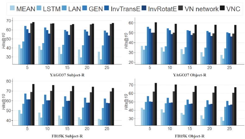
Figure 4. Link prediction results on YAGO37 and FB15K.

Tab. 2 and Fig. 4 show the experimental outcomes for the link prediction task. Based on the experimental results, we have the following observations: (i) Link predictions for OOKG entities are challenging, and for most baselines, the Hits@n and MRR are less than 0.7. In contrast, the proposed VNC is able to effectively infer missing fact triples for unseen entities. (ii) The proposed model VNC consistently outperforms state-of-the-art baselines and VN network over all the datasets. Compared to the baseline models, VNC achieves considerable increases in all metrics, including MR, MRR, Hits@10, Hits@3, and Hits@1. That is, identifying inter-rule correlations and capturing interactions among rule mining, rule inference, and embedding substantially enhance the performance for OOKG entities. (iii) When the ratio of the unseen entities increases and observed KGs become sparser, VNC is still able to accurately predict missing triples for OOKG entities. In Fig. 4, we show the results of link prediction experiments on datasets with different sample rates $R$. As the number of unseen entities increases, VNC still maintains the highest Hits@10 scores, indicating its robustness on sparse KGs. In summary, recognizing inter-rule correlations in KGs and designing an iterative framework for rule and embedding learning is able to strengthen the performance.

6.2. Triple classification (RQ1)

To further evaluate VNC, we conduct triple classification on the WN11 dataset. Based on the evaluation results in Tab. 3, we observe that VNC achieves state-of-the-art results on the triple classification task. With shallow pooling functions, MEAN and LSTM lead to the lowest accuracy. Meanwhile, other baseline models are hindered by the data sparsity problem, and ignoring complex patterns in graphs and interactions between rule and embedding learning. In contrast, VNC infers virtual neighbors for OOKG entities and mine logic rules and inter-rule correlations from KGs in an iterative manner, which results in the highest accuracies over all the datasets.

6.3. Comparisons with entity-independent methods (RQ1)

In addition to the entity-specific baselines, we compare VNC against entity-independent methods . Tab. 4 shows the evaluation results on FB15K Subject-10. We draw the following conclusions: (i) In comparison with entity-independent methods, the state-of-the-art entity-specific frameworks perform better, demonstrating the importance of embeddings of known entities. Compared to DRUM, GraIL, and TACT, entity-specific embedding models, including GEN, InvTransE, InvRotatE, VN network, and VNC, utilize pretrained embeddings of observed entities and attain huge performance enhancements. (ii) VNCoutperforms both entity-independent and entity-specific embedding methods, and achieves the best performance. This is, for OOKG entities, identifying inter-rule correlations in KGs and aggregating embeddings of neighborhood entities facilitate predictions of missing facts. In summary, extracting inter-rule correlations iteratively and integrating with embeddings of observed entities benefits the OOKG entity problem.

Table 2. Link prediction results on YAGO37 and FB15K. Significant improvements over the best baseline are marked with $\ast$ (t-test, $p<0.05$).

	YAGO37										FB15K
	Subject-10					Object-10					Subject-10					Object-10
Model	MR	MRR	Hits@10	Hits@3	Hits@1	MR	MRR	Hits@10	Hits@3	Hits@1	MR	MRR	Hits@10	Hits@3	Hits@1	MR	MRR	Hits@10	Hits@3	Hits@1
MEAN	2393	21.5	42.0	24.2	17.8	4763	17.8	35.2	17.5	12.1	293	31.0	48.0	34.8	22.2	353	25.1	41.0	28.0	17.1
LSTM	3148	19.4	37.9	20.3	15.9	5031	14.2	30.9	16.1	11.8	353	25.4	42.9	29.6	16.2	504	21.9	37.3	24.6	14.3
LAN	1929	24.7	45.4	26.2	19.4	4372	19.7	36.2	19.3	13.2	263	39.4	56.6	44.6	30.2	461	31.4	48.2	35.7	22.7
GEN	2259	46.9	62.5	52.5	39.3	4258	36.2	54.5	42.3	27.7	165	47.5	66.2	54.3	38.7	201	44.1	54.7	43.8	31.8
InvTransE	2308	44.9	59.7	50.2	37.7	4438	35.0	52.6	40.9	26.8	218	46.2	60.4	50.3	38.5	315	35.7	48.7	38.4	29.0
InvRotatE	2381	42.1	55.7	47.1	35.3	4518	32.5	48.7	37.6	24.9	233	45.3	60.4	50.2	36.9	276	36.2	49.1	38.6	29.3
VN network	1757	46.5	66.8	53.8	35.7	3145	27.4	50.1	36.4	19.5	175	46.3	70.1	52.6	34.5	212	42.3	62.7	44.6	28.2
VNC	1425∗	50.6∗	67.1	56.5∗	42.3∗	2638∗	39.1∗	59.1∗	45.8∗	30.1∗	151∗	54.3∗	75.9∗	60.8∗	41.6∗	183∗	48.2∗	70.5∗	52.9∗	36.3∗

Table 3. Triple classification results on WN11. Significant improvements over the best baseline are marked with $\ast$ (t-test, $p<0.05$).

	Subject			Object			Both
Model	1000	3000	5000	1000	3000	5000	1000	3000	5000
MEAN	87.3	84.3	83.3	84.0	75.2	69.2	83.0	73.3	68.2
LSTM	87.0	83.5	81.8	82.9	71.4	63.1	78.5	71.6	65.8
LAN	88.8	85.2	84.2	84.7	78.8	74.3	83.3	76.9	70.6
GEN	88.6	85.1	84.6	84.1	77.9	74.4	85.1	76.2	73.9
InvTransE	88.2	87.8	83.2	84.4	80.1	74.4	86.3	78.4	74.6
InvRotatE	88.4	86.9	84.1	84.6	80.1	74.9	84.2	75.0	70.6
VN network	89.1	85.9	85.4	85.5	80.6	76.8	84.1	78.5	73.1
VNC	90.6∗	88.9∗	86.7∗	86.9∗	82.3∗	78.3∗	87.7∗	79.6∗	76.2∗

Table 4. Link prediction results on FB15K Subject-10. Significant improvements over the best baseline are marked with $\ast$ (t-test, $p<0.05$).

Model	MR	MRR	Hits@10	Hits@3	Hits@1
DRUM	249	41.6	59.4	46.8	31.7
GraIL	241	41.9	60.1	47.3	32.1
TACT	238	42.6	60.2	47.1	32.9
VNC	151∗	54.3∗	75.9∗	60.8∗	41.6∗

7. Analysis

7.1. Ablation studies (RQ2)

To evaluate the effectiveness of each component in the VNC framework, we conduct ablation studies on the link prediction task. The results are shown in Tab. 5. When only employing the GNN-based encoder and embedding-based decoder (“no rules”), all metrics suffer a severe drop. In the “hard rules” setting, virtual neighbors are directly inferred by logic rules instead of soft label predictions. Compared to the “no rules” settings, predicting virtual neighbors with hard logic rules effectively alleviates the data sparsity problem. To examine the necessity of the iterative framework, we extract logic rules and learn knowledge embeddings simultaneously in the “soft rules” setting. The results show that the iterative framework captures interactions among rule mining, rule inference, and embedding, and gains considerable improvements over the model with hard logic rules. Moreover, compared with the “soft rules” setting, VNC further improves the performance by identifying inter-rule correlations in KG. In short, both inter-rule correlations and the iterative framework contribute to the improvements in performance. We also consider two model variants, VNC (AMIE+) and VNC (IterE), with different rule mining frameworks AMIE+ (Galárraga et al., 2015) and IterE (Zhang et al., 2019a), respectively. VNC (AMIE+) mines logic rules with AMIE+, and keeps confidence scores of logic rules unchanged during the training process. VNC (IterE) assumes the truth values of triples existing in KGs to be 1, and then calculates soft labels recursively using Eq. 8 instead of solving the optimization problem in Eq. 10. The results in Tab. 5 show that the proposed iterative framework in VNC outperforms other rule mining methods, indicating the effectiveness of VNC.

7.2. Influence of decoder (RQ3)

To assess the impact of various decoders on performance, we examine four types of embedding-based decoders, including TransE (Bordes et al., 2013), ConvE (Dettmers et al., 2018), Analogy (Liu et al., 2017), and DistMult (Yang et al., 2015), regarding their effectiveness in the link prediction task. According to the results in Tab. 6, VNC using the TransE decoder demonstrates the lowest performance, while VNC with DistMult achieves the highest performance. In comparison to translational models, the bilinear scoring function-based decoder is more compatible with our framework.

7.3. Case studies (RQ4)

For RQ4, we conduct case studies on VNC, and Tab. 7 shows examples of the inter-rule correlations on YAGO37. In the first example, from the logic rule and inter-rule path, it is easy to find that “George” is the director and producer of “Young Bess” and “Cass Timberlane”. Similarly, the second example shows that the children usually have the same citizenship as their parents. Note that, the above missing facts can not be directly inferred by either logic rules or symmetric path rules (He et al., 2020). Thus, by identifying useful inter-rule correlations, VNC is able to model complex patterns in the knowledge graph and facilitate embedding learning.

Table 5. Ablation studies on FB15K Subject-10.

Model	MR	MRR	Hits@10	Hits@3	Hits@1
VNC	151	54.3	75.9	60.8	41.6
No rules	251	40.9	61.9	47.3	31.5
Hard rules	192	45.2	67.6	52.6	35.4
Soft rules	164	53.3	74.2	58.5	40.1
VNC (AMIE+)	191	48.9	71.3	55.6	37.2
VNC (IterE)	172	52.5	73.7	58.8	39.7

Table 6. Influence of the decoders on FB15K Subject-10.

Decoder	MR	MRR	Hits@10	Hits@3	Hits@1
VN network	175	46.3	70.1	52.6	34.5
VNC (TransE)	204	47.4	71.2	53.6	34.5
VNC (ConvE)	171	53.1	74.6	59.8	41.2
VNC (Analogy)	163	52.9	74.8	60.1	40.7
VNC (DistMult)	151	54.3	75.9	60.8	41.6

Table 7. Examples of inter-rule correlations on YAGO37.

Soft label	$s($George, directed, Cass Timberlane$)=0.98$
Logic rule	$($George, directed, Young Bess$)\rightarrow$
	$($George, created, Young Bess$)$
Incomplete rule	$($George, directed, Cass Timberlane$)\rightarrow$
	$($George, created, Cass Timberlane$)$
Inter-rule path	$($Young Bess, isLocatedIn, United States$)\land$
	$($United States, isLocatedIn-1, Cass Timberlane$)$
Soft label	$s($Sigmar, isCitizenOf, Germany$)=0.92$
Logic rule	$($Thorbjørn, hasChild, Kjell$)\land($Kjell, isCitizenOf,
	Norway$)\rightarrow($Thorbjørn, isCitizenOf, Norway$)$
Incomplete rule	$($Franz, hasChild, Sigmar$)\land($Sigmar, isCitizenOf,
	Germany$)\rightarrow($Franz, isCitizenOf, Germany$)$
Inter-rule path	$($Germany, hasNeighbor, Denmark)
	${}\land($Denmark, dealWith, Norway$)$

8. Conclusion and future Work

In this paper, we focus on predicting missing facts for out-of-knowledge-graph (OOKG) entities. Previous work for this task still suffers from two key challenges: identifying inter-rule correlations, and capturing the interactions within rule and embedding learning. To address these problems, we propose a novel framework, named VNC, that infers virtual neighbors for OOKG entities by iteratively extracting logic rules and inter-rule correlations from knowledge graphs. We conduct both link prediction and triple classification, and experimental results show that the proposed VNC achieves state-of-the-art performance on four widely-used knowledge graphs. Besides, the VNC framework effectively alleviates the data sparsity problem, and is highly robust to the proportion of the unseen entities.

For future work, we plan to incorporate more kinds of complex patterns in knowledge graphs. In addition, generalizing the VNC framework to the unseen relations is also a promising direction.

- (1)
- Baek et al. (2020) Jinheon Baek, Dong Bok Lee, and Sung Ju Hwang. 2020. Learning to Extrapolate Knowledge: Transductive Few-shot Out-of-Graph Link Prediction. In NeurIPS.
- Bordes et al. (2013) Antoine Bordes, Nicolas Usunier, Alberto García-Durán, Jason Weston, and Oksana Yakhnenko. 2013. Translating Embeddings for Modeling Multi-relational Data. In NeurIPS. 2787–2795.
- Bordes et al. (2011) Antoine Bordes, Jason Weston, Ronan Collobert, and Yoshua Bengio. 2011. Learning Structured Embeddings of Knowledge Bases. In AAAI.
- Chen et al. (2021) Jiajun Chen, Huarui He, Feng Wu, and Jie Wang. 2021. Topology-Aware Correlations Between Relations for Inductive Link Prediction in Knowledge Graphs. In AAAI-IAAI. 6271–6278.
- Dai et al. (2021) Damai Dai, Hua Zheng, Fuli Luo, Pengcheng Yang, Tianyu Liu, Zhifang Sui, and Baobao Chang. 2021. Inductively Representing Out-of-Knowledge-Graph Entities by Optimal Estimation Under Translational Assumptions. In Proceedings of the 6th Workshop on Representation Learning for NLP, RepL4NLP@ACL-IJCNLP 2021, Online, August 6, 2021. 83–89.
- Dettmers et al. (2018) Tim Dettmers, Pasquale Minervini, Pontus Stenetorp, and Sebastian Riedel. 2018. Convolutional 2D Knowledge Graph Embeddings. In AAAI. 1811–1818.
- Ding et al. (2018) Boyang Ding, Quan Wang, Bin Wang, and Li Guo. 2018. Improving Knowledge Graph Embedding Using Simple Constraints. In ACL. 110–121.
- Galárraga et al. (2015) Luis Galárraga, Christina Teflioudi, Katja Hose, and Fabian M. Suchanek. 2015. Fast rule mining in ontological knowledge bases with AMIE+. VLDB J. 24, 6 (2015), 707–730.
- Galárraga et al. (2013) Luis Antonio Galárraga, Christina Teflioudi, Katja Hose, and Fabian M. Suchanek. 2013. AMIE: association rule mining under incomplete evidence in ontological knowledge bases. In WWW. 413–422.
- Graus et al. (2018) David Graus, Daan Odijk, and Maarten de Rijke. 2018. The Birth of Collective Memories: Analyzing Emerging Entities in Text Streams. Journal of the Association for Information Science and Technology 69, 6 (June 2018), 773–786.
- Guo et al. (2018) Shu Guo, Quan Wang, Lihong Wang, Bin Wang, and Li Guo. 2018. Knowledge Graph Embedding With Iterative Guidance From Soft Rules. In AAAI. 4816–4823.
- Hájek (1998) Petr Hájek. 1998. Metamathematics of Fuzzy Logic. Trends in Logic, Vol. 4.
- Hamaguchi et al. (2017) Takuo Hamaguchi, Hidekazu Oiwa, Masashi Shimbo, and Yuji Matsumoto. 2017. Knowledge Transfer for Out-of-Knowledge-Base Entities : A Graph Neural Network Approach. In IJCAI. 1802–1808.
- Hamilton et al. (2017) William L. Hamilton, Zhitao Ying, and Jure Leskovec. 2017. Inductive Representation Learning on Large Graphs. In NeurIPS. 1024–1034.
- He et al. (2017) He He, Anusha Balakrishnan, Mihail Eric, and Percy Liang. 2017. Learning Symmetric Collaborative Dialogue Agents with Dynamic Knowledge Graph Embeddings. In ACL. 1766–1776.
- He et al. (2020) Yongquan He, Zhihan Wang, Peng Zhang, Zhaopeng Tu, and Zhaochun Ren. 2020. VN Network: Embedding Newly Emerging Entities with Virtual Neighbors. In CIKM. 505–514.
- Kingma and Ba (2015) Diederik P. Kingma and Jimmy Ba. 2015. Adam: A Method for Stochastic Optimization. In ICLR.
- Lan and Jiang (2020) Yunshi Lan and Jing Jiang. 2020. Query Graph Generation for Answering Multi-hop Complex Questions from Knowledge Bases. In ACL. 969–974.
- Lin et al. (2015a) Yankai Lin, Zhiyuan Liu, Huan-Bo Luan, Maosong Sun, Siwei Rao, and Song Liu. 2015a. Modeling Relation Paths for Representation Learning of Knowledge Bases. In EMNLP. 705–714.
- Lin et al. (2015b) Yankai Lin, Zhiyuan Liu, Maosong Sun, Yang Liu, and Xuan Zhu. 2015b. Learning Entity and Relation Embeddings for Knowledge Graph Completion. In AAAI. 2181–2187.
- Liu et al. (2017) Hanxiao Liu, Yuexin Wu, and Yiming Yang. 2017. Analogical Inference for Multi-relational Embeddings. In ICML (Proceedings of Machine Learning Research, Vol. 70). 2168–2178.
- Min et al. (2013) Bonan Min, Ralph Grishman, Li Wan, Chang Wang, and David Gondek. 2013. Distant Supervision for Relation Extraction with an Incomplete Knowledge Base. In ACL. 777–782.
- Mu et al. (2021) Shanlei Mu, Yaliang Li, Wayne Xin Zhao, Siqing Li, and Ji-Rong Wen. 2021. Knowledge-Guided Disentangled Representation Learning for Recommender Systems. ACM Trans. Inf. Syst. 40, 1 (2021), 1–26.
- Neelakantan et al. (2015) Arvind Neelakantan, Benjamin Roth, and Andrew McCallum. 2015. Compositional Vector Space Models for Knowledge Base Completion. In ACL-IJCNLP. 156–166.
- Nickel et al. (2011) Maximilian Nickel, Volker Tresp, and Hans-Peter Kriegel. 2011. A Three-Way Model for Collective Learning on Multi-Relational Data. In ICML. 809–816.
- Niu et al. (2020) Guanglin Niu, Yongfei Zhang, Bo Li, Peng Cui, Si Liu, Jingyang Li, and Xiaowei Zhang. 2020. Rule-Guided Compositional Representation Learning on Knowledge Graphs. In AAAI-IAAI. 2950–2958.
- Omran et al. (2018) Pouya Ghiasnezhad Omran, Kewen Wang, and Zhe Wang. 2018. Scalable Rule Learning via Learning Representation. In IJCAI. 2149–2155.
- Sadeghian et al. (2019) Ali Sadeghian, Mohammadreza Armandpour, Patrick Ding, and Daisy Zhe Wang. 2019. DRUM: End-To-End Differentiable Rule Mining On Knowledge Graphs. In NeurIPS. 15321–15331.
- Schlichtkrull et al. (2018) Michael Sejr Schlichtkrull, Thomas N. Kipf, Peter Bloem, Rianne van den Berg, Ivan Titov, and Max Welling. 2018. Modeling Relational Data with Graph Convolutional Networks. In ESWC, Vol. 10843. 593–607.
- Shang et al. (2019) Chao Shang, Yun Tang, Jing Huang, Jinbo Bi, Xiaodong He, and Bowen Zhou. 2019. End-to-End Structure-Aware Convolutional Networks for Knowledge Base Completion. In AAAI. 3060–3067.
- Shi and Weninger (2018) Baoxu Shi and Tim Weninger. 2018. Open-World Knowledge Graph Completion. In AAAI-IAAI. 1957–1964.
- Socher et al. (2013) Richard Socher, Danqi Chen, Christopher D. Manning, and Andrew Y. Ng. 2013. Reasoning With Neural Tensor Networks for Knowledge Base Completion. In NeurIPS. 926–934.
- Sun et al. (2019) Zhiqing Sun, Zhi-Hong Deng, Jian-Yun Nie, and Jian Tang. 2019. RotatE: Knowledge Graph Embedding by Relational Rotation in Complex Space. In ICLR.
- Teru et al. (2020) Komal K. Teru, Etienne Denis, and Will Hamilton. 2020. Inductive Relation Prediction by Subgraph Reasoning. In ICML. 9448–9457.
- Wang et al. (2018) Guanying Wang, Wen Zhang, Ruoxu Wang, Yalin Zhou, Xi Chen, Wei Zhang, Hai Zhu, and Huajun Chen. 2018. Label-Free Distant Supervision for Relation Extraction via Knowledge Graph Embedding. In EMNLP. 2246–2255.
- Wang et al. (2019d) Hongwei Wang, Fuzheng Zhang, Jialin Wang, Miao Zhao, Wenjie Li, Xing Xie, and Minyi Guo. 2019d. Exploring High-Order User Preference on the Knowledge Graph for Recommender Systems. ACM Trans. Inf. Syst. 37, 3 (2019), 32:1–32:26.
- Wang et al. (2022) Liang Wang, Wei Zhao, Zhuoyu Wei, and Jingming Liu. 2022. SimKGC: Simple Contrastive Knowledge Graph Completion with Pre-trained Language Models. In ACL. 4281–4294.
- Wang et al. (2019a) Peifeng Wang, Jialong Han, Chenliang Li, and Rong Pan. 2019a. Logic Attention Based Neighborhood Aggregation for Inductive Knowledge Graph Embedding. In AAAI-IAAI. 7152–7159.
- Wang et al. ([n. d.]) Shen Wang, Xiaokai Wei, Cícero Nogueira dos Santos, Zhiguo Wang, Ramesh Nallapati, Andrew O. Arnold, Bing Xiang, Philip S. Yu, and Isabel F. Cruz. [n. d.]. Mixed-Curvature Multi-Relational Graph Neural Network for Knowledge Graph Completion. In WWW. 1761–1771.
- Wang et al. (2021) Xiaozhi Wang, Tianyu Gao, Zhaocheng Zhu, Zhengyan Zhang, Zhiyuan Liu, Juanzi Li, and Jian Tang. 2021. KEPLER: A Unified Model for Knowledge Embedding and Pre-trained Language Representation. Trans. Assoc. Comput. Linguistics 9 (2021), 176–194.
- Wang et al. (2019b) Xiang Wang, Xiangnan He, Yixin Cao, Meng Liu, and Tat-Seng Chua. 2019b. KGAT: Knowledge Graph Attention Network for Recommendation. In SIGKDD. 950–958.
- Wang et al. (2019c) Zihan Wang, Zhaochun Ren, Chunyu He, Peng Zhang, and Yue Hu. 2019c. Robust Embedding with Multi-Level Structures for Link Prediction. In IJCAI. 5240–5246.
- Wang et al. (2014) Zhen Wang, Jianwen Zhang, Jianlin Feng, and Zheng Chen. 2014. Knowledge Graph Embedding by Translating on Hyperplanes. In AAAI. 1112–1119.
- Xu et al. (2015) Bing Xu, Naiyan Wang, Tianqi Chen, and Mu Li. 2015. Empirical Evaluation of Rectified Activations in Convolutional Network. CoRR abs/1505.00853 (2015).
- Yang et al. (2015) Bishan Yang, Wen-tau Yih, Xiaodong He, Jianfeng Gao, and Li Deng. 2015. Embedding Entities and Relations for Learning and Inference in Knowledge Bases. In ICLR.
- Yang et al. (2021) Tianchi Yang, Linmei Hu, Chuan Shi, Houye Ji, Xiaoli Li, and Liqiang Nie. 2021. HGAT: Heterogeneous Graph Attention Networks for Semi-supervised Short Text Classification. ACM Trans. Inf. Syst. 39, 3 (2021), 32:1–32:29.
- Zhang et al. (2018) Maoyuan Zhang, Qi Wang, Wukui Xu, Wei Li, and Shuyuan Sun. 2018. Discriminative Path-Based Knowledge Graph Embedding for Precise Link Prediction. In ECIR (Lecture Notes in Computer Science, Vol. 10772). 276–288.
- Zhang et al. (2019b) Richong Zhang, Yue Wang, Yongyi Mao, and Jinpeng Huai. 2019b. Question Answering in Knowledge Bases: A Verification Assisted Model with Iterative Training. ACM Trans. Inf. Syst. 37, 4 (2019), 40:1–40:26.
- Zhang et al. (2019a) Wen Zhang, Bibek Paudel, Liang Wang, Jiaoyan Chen, Hai Zhu, Wei Zhang, Abraham Bernstein, and Huajun Chen. 2019a. Iteratively Learning Embeddings and Rules for Knowledge Graph Reasoning. In WWW. 2366–2377.
- Zhang et al. (2021) Yufeng Zhang, Weiqing Wang, Wei Chen, Jiajie Xu, An Liu, and Lei Zhao. 2021. Meta-Learning Based Hyper-Relation Feature Modeling for Out-of-Knowledge-Base Embedding. In CIKM. 2637–2646.