Edge Directionality Improves Learning on Heterophilic Graphs

Abstract

Graph Neural Networks (GNNs) have become the de-facto standard tool for modeling relational data. However, while many real-world graphs are directed, the majority of today’s GNN models discard this information altogether by simply making the graph undirected. The reasons for this are historical: 1) many early variants of spectral GNNs explicitly required undirected graphs, and 2) the first benchmarks on homophilic graphs did not find significant gain from using direction. In this paper, we show that in heterophilic settings, treating the graph as directed increases the effective homophily of the graph, suggesting a potential gain from the correct use of directionality information. To this end, we introduce Directed Graph Neural Network (Dir-GNN), a novel general framework for deep learning on directed graphs. Dir-GNN can be used to extend any Message Passing Neural Network (MPNN) to account for edge directionality information by performing separate aggregations of the incoming and outgoing edges. We prove that Dir-GNN matches the expressivity of the Directed Weisfeiler-Lehman test, exceeding that of conventional MPNNs. In extensive experiments, we validate that while our framework leaves performance unchanged on homophilic datasets, it leads to large gains over base models such as GCN, GAT and GraphSage on heterophilic benchmarks, outperforming much more complex methods and achieving new state-of-the-art results. The code for the paper can be found at https://github.com/emalgorithm/directed-graph-neural-network.

1 Introduction

Graph Neural Networks (GNNs) have demonstrated remarkable success across a wide range of problems and fields [1]. Most GNN models, however, assume that the input graph is undirected [2, 3, 4], despite the fact that many real-world networks, such as citation and social networks, are inherently directed. Applying GNNs to directed graphs often involves either converting them to undirected graphs or only propagating information over incoming (or outgoing) edges, both of which may discard valuable information crucial for downstream tasks.

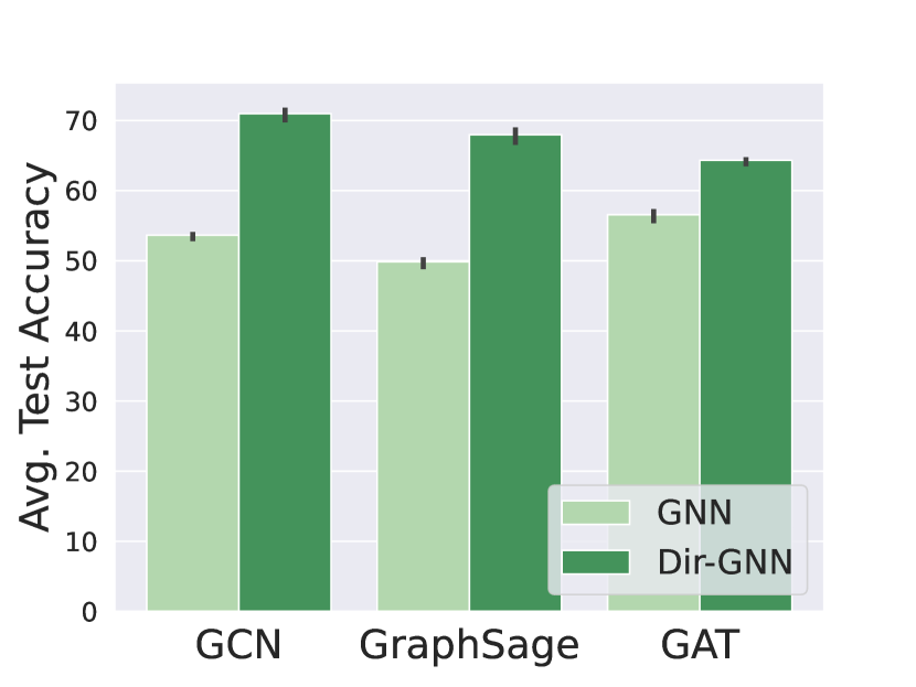
(a) Heterophilic Graphs

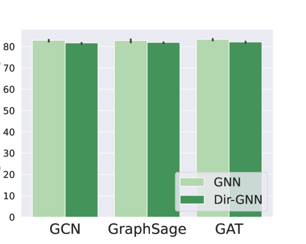
(b) Homophilic Graphs

Figure 1: Extending popular GNN architectures with our Dir-GNN framework to incorporate edge-directionality information brings large gains ($10\%$ to $15\%$) on heterophilic datasets (left), while leaving performance mostly unchanged on homophilic datasets (right). The plots illustrate the average performance over all datasets, while the full results are presented in Tab. 2.

We believe the dominance of undirected graphs in the field is rooted in two “original sins” of GNNs. First, undirected graphs have symmetric Laplacians which admit orthogonal eigendecomposition. Orthogonal Laplacian eigenvectors act as a natural generalization of the Fourier transform and allow to express graph convolution operations in the Fourier domain. Since some of the early graph neural networks originated from the field of graph signal processing [5, 6], the undirected graph assumption was necessary for spectral GNNs [7, 8, 2] to be properly defined. With the emergence of spatial GNNs, unified with the message-passing framework (MPNNs [9]), this assumption was not strictly required anymore, as MPNNs can easily be applied to directed graphs by propagating over the directed adjacency, resulting however in information being propagated only in a single direction, at the risk of discarding useful information from the opposite one. However, early works empirically observed that making the graph undirected consistently leads to better performance on established node-classification benchmarks, which historically have been mainly homophilic graphs such as Cora and Pubmed [10], where neighbors tend to share the same label. Consequently, converting input graphs to undirected ones has become a standard part of the dataset preprocessing pipeline, to the extent that the popular GNN library PyTorch-Geometric [11] includes a general utility function that automatically makes graphs undirected when loading datasets.

The key observation in this paper is that while accounting for edge directionality indeed does not help in homophilic graphs, it can bring extensive gains in heterophilic settings (Fig. 1), where neighbors tend to have different labels. In the rest of the paper, we study why and how to use directionality to improve learning on heterophilic graphs.

Contributions. Our contributions are the following:

• We show that considering the directionality of a graph substantially increases its effective homophily in heterophilic settings, with negligible or no impact on homophilic settings (see Sec. 3).

• We propose a novel and generic Directed Graph Neural Network framework (Dir-GNN) which extends any MPNN to work on directed graphs by performing separate aggregations of the incoming and outgoing edges. Moreover, we show that Dir-GNN leads to more homophilic aggregations compared to their undirected counterparts (see Sec. 4).

• Our theoretical analysis establishes that Dir-GNN is as expressive as the Directed Weisfeiler-Lehman test, while being strictly more expressive than MPNNs (see  Sec. 4.1).

• We empirically validate that augmenting popular GNN architectures with the Dir-GNN framework yields large improvements on heterophilic benchmarks, achieving state-of-the-art results and outperforming even more complex methods specifically designed for such settings. Moreover, this enhancement does not negatively impact the performance on homophilic benchmarks (see Sec. 6).

2 Background

We consider a directed graph $G=(V,E)$ with a node set $V$ of $n$ nodes, and an edge set $E$ of $m$ edges. We define its respective directed adjacency matrix $\mathbf{A}\in\{0,1\}^{n\times n}$ where $a_{ij}=1$ if $(i,j)\in E$ and zero otherwise, its respective undirected adjacency matrix $\mathbf{A}_{u}$ where $(a_{u})_{ij}=1$ if $(i,j)\in E$ or $(j,i)\in E$ and zero otherwise. In this paper, we focus on the task of (semi-supervised) node classification on an attributed graph $G$ with node features arranged into the $n\times d$ matrix $\mathbf{X}$ and node labels $y_{i}\in\{1,...,C\}$.

2.1 Homophily and Heterophily in Undirected Graphs

In this Section, we first review the heterophily metrics for undirected graphs, while in Sec. 3 we propose heterophily metrics adapted to directed graphs. Most GNNs are based on the homophily assumption for undirected graphs, i.e., that neighboring nodes tend to share the same labels. While a reasonable assumption in some settings, it turns out not to be true in many important applications such as gender classification on social networks or fraudster detection on e-commerce networks.

Homophily metrics. Several metrics have been proposed to measure homophily on undirected graphs. Node homophily is defined as

$$h=\frac{1}{|V|}\sum_{i\in V}\frac{\sum_{j:(i,j)\in E}I[y_{i}=y_{j}]}{d_{i}}$$ (1)

where $I[y_{i}=y_{j}]$ is the indicator function with value 1 if $y_{i}=y_{j}$ or zero otherwise. Intuitively, node homophily measures the fraction of neighbors with the same label as the node itself, averaged across all nodes. However, since heterophily is a complex phenomenon which is hard to capture with only a single scalar, a better representation of a graph’s homophily is the $C\times C$ class compatibility matrix $\mathbf{H}$ [12], capturing the fraction of edges from nodes with label $k$ to nodes with label $l$:

$$h_{kl}=\frac{|(i,j)\in E:y_{i}=k\land y_{j}=l|}{|(i,j)\in E:y_{i}=k|}.$$

Homophilic datasets are expected to have most of the mass of their compatibility matrices concentrated in the diagonal, as most of the edges are between nodes of the same class (e.g. see Citeseer-Full in Fig. 3). Conversely, heterophilic datasets will have most of the mass away from the diagonal of the compatibility matrix (e.g. see Chameleon in Fig. 3).

2.2 Message Passing Neural Network

In this Section, we first review the Message Passing Neural Network (MPNN) paradigm for undirected graphs, while in Sec. 4 we extend this formalism to directed graphs. An MPNN is a parametric model which iteratively applies aggregation maps $\mathrm{AGG}^{(k)}$ and combination maps $\mathrm{COM}^{(k)}$ to compute embeddings $\mathbf{x}_{i}^{(k)}$ for node $i$ based on messages $\mathbf{m}^{(k)}_{i}$ containing information on its neighbors. Namely, the $k$-th layer of an MPNN is given by

$$\begin{split}\mathbf{m}^{(k)}_{i}&=\mathrm{AGG}^{(k)}\left(\{\mskip-6.0mu\{(\mathbf{x}_{j}^{(k-1)},\mathbf{x}_{i}^{(k-1)}):\,(i,j)\in E\}\mskip-6.0mu\}\right)\\ \mathbf{x}_{i}^{(k)}&=\mathrm{COM}^{(k)}\left(\mathbf{x}_{i}^{(k-1)},\mathbf{m}^{(k)}_{i}\right)\end{split}$$ (2)

where $\{\mskip-6.0mu\{\cdot\}\mskip-6.0mu\}$ is a multi-set. The aggregation maps $\mathrm{AGG}^{(k)}$ and the combination maps $\mathrm{COM}^{(k)}$ are learnable (usually a small neural network) and their different implementations result in specific architectures (e.g. graph convolutional neural networks (GCN) use linear aggregation, graph attention networks (GAT) use attentional layers, etc.). After the last layer $K$, the node representation $\mathbf{x}_{i}^{(K)}$ is mapped into the $C$-probability simplex via a (learnable) decoding step, often given by an MLP. Independent of the choice of $\mathrm{AGG}$ and $\mathrm{COM}$, all MPNNs only send messages along the edges of the graph, which make them particularly suitable for tasks where edges do encode a notion of similarity – as it is the case when adjacent nodes in the graph often share the same label (homophilic). Conversely, MPNNs tend to struggle in the scenario where they need to separate a node embedding from that of its neighbours [13], often a challenging problem that has gained attention in the community and which we discuss in detail next.

3 Heterophily in Directed Graphs

In this Section, we discuss how accounting for directionality can be particularly helpful for dealing with heterophilic graphs. By leveraging the directionality information, we argue that even standard MPNNs that are traditionally thought to struggle in the heterophilic regime, can in fact perform extremely well.

Weighted homophily metrics. First, we extend the homophily metrics introduced in Section 2.1 to account for directed edges and higher-order neighborhoods. Given a possibly directed and weighted $n\times n$ message-passing matrix $\mathbf{S}$, we define the weighted node homophily as

$$h(\mathbf{S})=\frac{1}{|V|}\sum_{i\in V}\frac{\sum_{j\in V}s_{ij}I[y_{i}=y_{j}]}{\sum_{j\in V}s_{ij}}$$ (3)

Accordingly, by taking $\mathbf{S}=\mathbf{A}$ and $\mathbf{S}=\mathbf{A}^{\top}$ respectively, we can compute the node homophily based on outgoing or incoming edges. Similarly, we can also take $\mathbf{S}$ to be any weighted 2-hop matrix associated with a directed graph (see details below) and compute its node homophily.

We can also extend the construction to edge-computations by defining the $C\times C$ weighted compatibility matrix $\mathbf{H}(\mathbf{S})$ of a message-passing matrix $\mathbf{S}$ as

$$h_{kl}(\mathbf{S})=\frac{\sum_{i,j\in V:y_{i}=k\land y_{j}=l}s_{ij}}{\sum_{i,j\in V:y_{i}=k}s_{ij}}$$ (4)

As above, one can take $\mathbf{S}=\mathbf{A}$ or $\mathbf{S}=\mathbf{A}^{\top}$ to derive the compatibility matrix associated with the out and in-edges, respectively.

Effective homophily. Stacking multiple layers of a GNN effectively corresponds to taking powers of diffusion matrices, resulting in message propagation over higher-order hops. Zhu et al. [12] noted that for heterophilic graphs, the 2-hop tends to be more homophilic than the 1-hop. This phenomenon of similarity within “friends-of-friends” has been widely observed and is commonly referred to as monophily [14]. If higher-order hops exhibit increased homophily, exploring the graph through layers can prove beneficial for the task. Consequently, we introduce the concept of effective homophily as the maximum weighted node homophily observable at any hop of the graph.

For directed graphs, there exists an exponential number of $k$-hops. For instance, four 2-hop matrices can be considered: the squared operators $\mathbf{A}^{2}$ and $(\mathbf{A}^{\top})^{2}$, which correspond to following the same forward or backward edge direction twice, as well as the non-squared operators $\mathbf{A}\mathbf{A}^{\top}$ and $\mathbf{A}^{\top}\mathbf{A}$, representing the forward/backward and backward/forward edge directions. Given a graph $G$, we define its effective homophily as follows:

$$h^{(\text{eff})}=\max_{k\geq 1}\max_{\mathbf{C}\in\mathcal{B}^{k}}h(\mathbf{C})$$ (5)

where $\mathcal{B}^{k}$ denotes the set of all $k$-hop matrices for a graph. If $G$ is undirected, $\mathcal{B}^{k}$ contains only $\mathbf{A}^{k}$. In our empirical analysis, we will focus on the 2-hop matrices, as computing higher-order $k$-hop matrices becomes intractable for all but the smallest graphs .

		$\mathbf{A}_{u}$	$\mathbf{A}_{u}^{2}$	$h^{(\text{eff})}_{u}$	$\mathbf{A}$	$\mathbf{A}^{\top}$	$\mathbf{A}^{\top}\mathbf{A}$	$\mathbf{A}\mathbf{A}^{\top}$	$h^{(\text{eff})}_{d}$	$h^{(\text{eff})}_{\text{gain}}$
Homophilic	citeseer-full	0.958	0.951	0.958	0.954	0.959	0.971	0.951	0.971	1.36%
	cora-ml	0.810	0.767	0.810	0.808	0.833	0.803	0.779	0.833	2.84%
	ogbn-arxiv	0.635	0.548	0.635	0.632	0.675	0.658	0.556	0.675	6.3%
Heterophilic	chameleon	0.248	0.331	0.331	0.249	0.274	0.383	0.335	0.383	15.71%
	squirrel	0.218	0.252	0.252	0.219	0.210	0.257	0.258	0.258	2.38%
	arxiv-year	0.289	0.397	0.397	0.310	0.403	0.487	0.431	0.487	22.67%
	snap-patents	0.221	0.372	0.372	0.266	0.271	0.478	0.522	0.522	40.32%
	roman-empire	0.046	0.365	0.365	0.045	0.042	0.535	0.609	0.609	66.85%

Table 1: Weighted node homophily for different diffusion matrices, and effective homophily for both undirected ($h^{(\text{eff})}_{u}$) and directed graph ($h^{(\text{eff})}_{d}$). The last column reports the gain in effective homophily obtained by using the directed graph as opposed to the undirected graph.

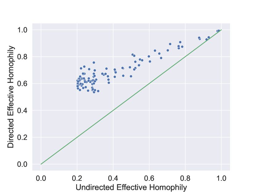
(a)

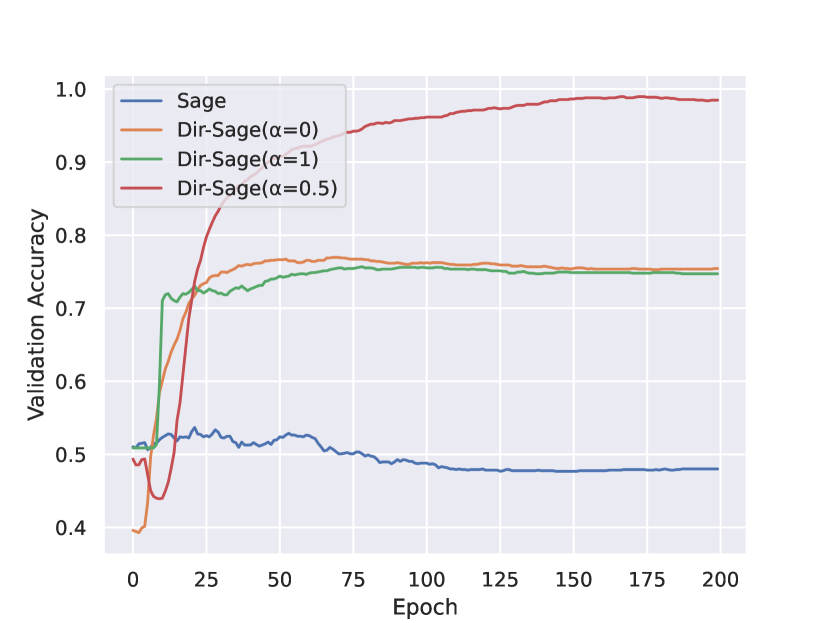
(b)

Figure 2: In our synthetic experiments, we observe the following: (a) the effective homophily of directed graphs is consistently higher compared to their undirected counterparts. Interestingly, this gap widens for graphs that are less homophilic. (b) When examining the performance of GraphSage and its Dir-GNN extensions on a synthetic task requiring directionality information, only Dir-Sage($\alpha$=0.5), which utilizes information from both directions, is capable of solving the task.

Leveraging directionality to enhance effective homophily. We observe that converting a graph from directed to undirected results in lower effective homophily for heterophilic graphs, while the impact on homophilic graphs is negligible (refer to the last column of Tab. 1). Specifically, $\mathbf{A}\mathbf{A}^{\top}$ and $\mathbf{A}^{\top}\mathbf{A}$ emerge as the most homophilic diffusion matrices for heterophilic graphs. In fact, the average relative gain of effective homophily, $h^{(\text{eff})}_{\text{gain}}$, when using directed graphs compared to undirected ones is only around $3\%$ for homophilic datasets, while it is almost $30\%$ for heterophilic datasets. We further validate this observation on synthetic directed graphs exhibiting various levels of homophily, generated through a modified preferential attachment process (see Sec. H.1 for more details). Fig. 2(a) displays the results: the directed graph consistently demonstrates higher effective homophily compared to its undirected counterpart, with the gap being particularly prominent for lower node homophily levels. The minimal effective homophily gain on homophilic datasets further substantiates the traditional practice of using undirected graphs for benchmarking GNNs, as the datasets were predominantly homophilic until recently.

Real-world example. We illustrate the concept of effective homophily in heterophilic directed graphs by taking the concrete task of predicting the publication year of papers based on a directed citation network such as Arxiv-Year [15]. In this case, the different 2-hop neighbourhoods have very different semantics: the diffusion operator $(\mathbf{A}^{2})_{i}$ represents papers that are cited by those papers that paper $i$ cites. As these 2-hop neighboring papers were published further in the past relative to paper $i$, they do not offer much information about the publication year of $i$. On the other hand, $(\mathbf{A}^{\top}\mathbf{A})_{i}$ represents papers that share citations with paper $i$. Papers cited by the same sources are more likely to have been published in the same period, so the diffusion operator $\mathbf{A}^{\top}\mathbf{A}$ is expected to be more homophilic. The undirected 2-hop operator $\mathbf{A}_{u}^{2}=(\frac{1}{2}(\mathbf{A}+\mathbf{A}^{\top}))^{2}=\frac{1}{4}(\mathbf{A}^{2}+(\mathbf{A}^{\top})^{2}+\mathbf{A}\mathbf{A}^{\top}+\mathbf{A}\mathbf{A}^{\top})$ is the average of the four directed 2-hops. Therefore, the highly homophilic matrix $\mathbf{A}^{\top}\mathbf{A}$ is diluted by the inclusion of $(\mathbf{A}^{2})$, leading to a less homophilic operator overall.

4 Directed Graph Neural Network

In this Section, we extend the class of MPNNs to directed graphs, and refer to such generalization as Directed Graph Neural Network (Dir-GNN). We follow the scheme in Eq. 2, meaning that the update of a node feature is the result of a combination of its previous state and an aggregation over its neighbours. Crucially though, the characterization of neighbours now has to account for the edge-directionality. Accordingly, given a node $i\in V$, we perform separate aggregations over the in-neighbours ($j\rightarrow i$) and the out-neighbours ($i\rightarrow j$) respectively:

$$\begin{split}\mathbf{m}^{(k)}_{i,\leftarrow}&=\mathrm{AGG}^{(k)}_{\leftarrow}\left(\{\mskip-6.0mu\{(\mathbf{x}_{j}^{(k-1)},\mathbf{x}_{i}^{(k-1)}):\,(j,i)\in E\}\mskip-6.0mu\}\right)\\ \mathbf{m}^{(k)}_{i,\rightarrow}&=\mathrm{AGG}^{(k)}_{\rightarrow}\left(\{\mskip-6.0mu\{(\mathbf{x}_{j}^{(k-1)},\mathbf{x}_{i}^{(k-1)}):\,(i,j)\in E\}\mskip-6.0mu\}\right)\\ \mathbf{x}_{i}^{(k)}&=\mathrm{COM}^{(k)}\left(\mathbf{x}_{i}^{(k-1)},\mathbf{m}^{(k)}_{i,\leftarrow},\mathbf{m}^{(k)}_{i,\rightarrow}\right).\end{split}$$ (6)

The idea behind our framework is that given any MPNN, we can readily adapt it to the directed case by choosing how to aggregate over both directions. For this purpose, we replace the neighbour aggregator $\mathrm{AGG}^{(k)}$ with two separate in- and out-aggregators $\mathrm{AGG}^{(k)}_{\leftarrow}$ and $\mathrm{AGG}^{(k)}_{\rightarrow}$, which can have independent sets of parameters for the two aggregation phases and, possibly, different normalizations as discussed below – however the functional expression in both cases stays the same. As we will show, accounting for both directions separately is fundamental for both the expressivity of the model (see Sec. 4.1) and its empirical performance (see Sec. 6.1).

Extension of common architectures. To make our discussion more explicit, we describe extensions of popular MPNNs where the aggregation map is computed by $\mathbf{m}^{(k)}_{i}=(\mathbf{S}\mathbf{x}^{(k-1)})_{i}$, where $\mathbf{S}\in\mathbb{R}^{n\times n}$ is a message-passing matrix. In GCN [2], $\mathbf{S}=\mathbf{D}^{-1/2}\mathbf{A}_{u}\mathbf{D}^{-1/2}$, where $\mathbf{D}$ is the degree matrix of the undirected graph. In the case of directed graphs, two message-passing matrices $\mathbf{S}_{\leftarrow}$ and $\mathbf{S}_{\rightarrow}$ are required for in- and out-neighbours respectively. Additionally, the normalization is slightly more subtle, since we now have two different diagonal degree matrices $\mathbf{D}_{\leftarrow}$ and $\mathbf{D}_{\rightarrow}$ containing the in-degrees and out-degrees respectively. Accordingly, we propose a normalization of the form $\mathbf{S}_{\rightarrow}=\mathbf{D}_{\rightarrow}^{-1/2}\mathbf{A}\mathbf{D}_{\leftarrow}^{-1/2}$ i.e. $(\mathbf{S}_{\rightarrow})_{ij}=a_{ij}/\sqrt{d^{\rightarrow}_{i}d^{\leftarrow}_{j}}$. To motivate this choice, note that the normalization modulates the aggregation based on the out-degree of $i$ and the in-degree of $j$ as one would expect given that we are computing a message going from $i$ to $j$. We can then take $\mathbf{S}_{\leftarrow}=\mathbf{S}_{\rightarrow}^{\top}$ and write the update at layer $k$ of Dir-GCN as

$$\mathbf{X}^{(k)}=\sigma\left(\mathbf{S}_{\rightarrow}\mathbf{X}^{(k-1)}\mathbf{W}^{(k)}_{\rightarrow}+\mathbf{S}^{\top}_{\rightarrow}\mathbf{X}^{(k-1)}\mathbf{W}^{(k)}_{\leftarrow}\right),$$ (7)

for learnable channel-mixing matrices $\mathbf{W}^{(k)}_{\rightarrow},\mathbf{W}^{(k)}_{\leftarrow}$ and with $\sigma$ a pointwise activation map. Finally, we note that in our implementation of Dir-GNN we use an additional learnable or tunable parameter $\alpha$ allowing the framework to weight one direction more than the other (a convex combination), depending on the dataset. Dir-GNN extensions of GAT [3] and GraphSAGE [4] can be found in Appendix C.

Dir-GNN leads to more homophilic aggregations. Since our main application amounts to relying on the graph-directionality to mitigate heterophily, here we comment on how information is iteratively propagated in a Dir-GNN, generally leading to an aggregation scheme beneficial on most real-world directed heterophilic graphs. We focus on the Dir-GCN formulation, however the following applies to any other Dir-GNN up to changing the message-passing matrices. Consider a 2-layer Dir-GCN as in Eq. 7, and let us remove the pointwise activation $\sigma$ . Then, the node representation can be written as

We observe that when we aggregate information over multiple layers, the final node representation is derived by also computing convolutions over 2-hop matrices $\mathbf{A}_{\rightarrow}^{\top}\mathbf{A}_{\rightarrow}$ and $\mathbf{A}_{\rightarrow}\mathbf{A}^{\top}_{\rightarrow}$. From the discussion in Sec. 3, we deduce that this framework may be more suited to handle heterophilic graphs since generally such 2-hop matrices are more likely to encode similarity than $\mathbf{A}_{\rightarrow}^{2}$, $(\mathbf{A}_{\rightarrow}^{\top})^{2}$ or $\mathbf{A}_{u}^{2}$ – this is validated empirically on real-world datasets in Sec. 6.

Advantages of two-directional updates. We discuss the benefits of incorporating both directions in the layer update, as opposed to using a single direction. Although spatial MPNNs can be adapted to directed graphs by simply utilizing $\mathbf{A}$ instead of $\mathbf{A}_{u}$—resulting in message propagation only along out-edges—relying on a single direction presents three primary drawbacks. First, if the layer update only considers one direction, the exploration of the multi-hop neighbourhoods through powers of diffusion operators would not include the mixed terms $\mathbf{A}\mathbf{A}^{\top}$ and $\mathbf{A}^{\top}\mathbf{A}$, which have been shown to be particularly beneficial for heterophilic graphs in Sec. 3. Second, by using only one direction we disregard the graph entirely for nodes where the out-degree is zero . This phenomenon frequently occurs in real-world graphs, as reported in Tab. 9. Incorporating both directions in the layer update helps mitigate this problem, as it is far less common for a node to have both in- and out-degree to be zero, as also illustrated in Tab. 9. Third, limiting the update to a single direction reduces expressivity, as we discuss in Sec. 4.1.

Complexity. The complexity of Dir-GNN depends on the specific instantiation of the framework. Dir-GCN, Dir-Sage, and Dir-GAT maintain the same per-layer computational complexity as their undirected counterparts ($\mathcal{O}(md+nd^{2})$ for GCN and GraphSage, and $\mathcal{O}(md^{2})$ for GAT). However, they have twice as many parameters, owing to their separate weight matrices for in- and out-neighbors.

4.1 Expressive power of Dir-GNN

It is a well known result that MPNNs are bound in expressivity by the 1-WL test, and that it is possible to construct MPNN models which are as expressive as the 1-WL test [17]. In this section, we show that Dir-GNN is the optimal way to extend MPNNs to directed graphs. We do so by proving that Dir-GNN models can be constructed to be as expressive as an extension of the 1-WL test to directed graphs [18], referred to as D-WL (for a formal definition, see Sec. D.1). Additionally, we illustrate its greater expressivity over more straightforward approaches, such as converting the graph to its undirected form and utilizing a standard MPNN (MPNN-U) or applying an MPNN that propagates solely along edge direction (MPNN-D). Formal statements for the theorems in this section along with their proofs can be found in Appendix D.

Theorem 4.1 (Informal).

Dir-GNN is as expressive as D-WL if $\mathrm{AGG}^{(k)}_{\rightarrow}$, $\mathrm{AGG}^{(k)}_{\leftarrow}$, and $\mathrm{COM}^{(k)}$ are injective for all $k$.

A discussion of how a Dir-GNN can be parametrized to meet these conditions (similarly to what is done in Xu et al. [17]) can be found in Sec. D.4.

Theorem 4.2 (Informal).

Dir-GNN is strictly more expressive than both MPNN-U and MPNN-D.

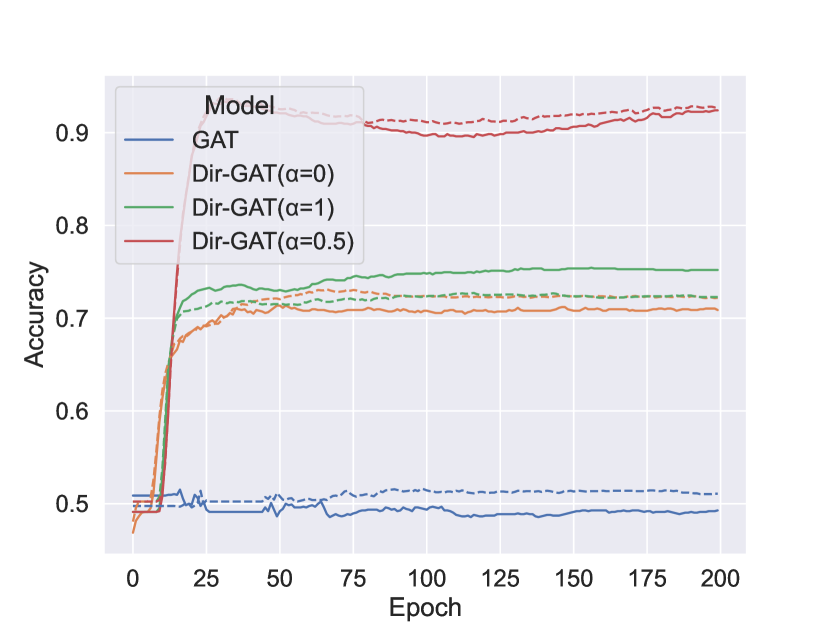
Figure 9: Validation accuracy (solid lines) and training accuracy (dashed lines) of GCN (left) and GAT (right), as well as their respective extensions using our Dir-GNN framework, on a synthetic task which requires directionality information in order to be solved.

Intuitively, the theorem states that while all directed graphs distinguished by MPNNs are also separated by Dir-GNNs, there also exist directed graphs separated by the latter but not by the former. This holds true for MPNNs applied both on the directed and undirected graph. We observe these theoretical findings to be in line with the empirical results detailed in Fig. 9 and Tab. 10, where Dir-GNN performs comparably or better (typically in the case of heterophily) than MPNNs.

5 Related Work

GNNs for directed graphs. While several classical papers have alluded to the extension of their spatial models to directed graphs, empirical validation has not been conducted [19, 20, 9]. GatedGCN [21] deals with directed graphs, however it aggregates information only from out-neighbors, neglecting potentially valuable information from in-neighbors. More recently, Vrček et al. [22] tackle the genome assembly problem by employing a GatedGCN with separate aggregations for in- and out-neighbors. Various approaches have been developed to generalize spectral convolutions for directed graphs [23, 24]. Of particular interest are DGCN [25], which leverages $\mathbf{A}^{\top}\mathbf{A}$ and $\mathbf{A}\mathbf{A}^{\top}$ for its convolution (see Appendix G for a more detailed comparison with Dir-GNN), DiGCN [26], which uses Personalized Page Rank matrix as a generalized Laplacian and incorporates $k$-hop diffusion matrices, and MagNet [27], which adopts a complex matrix for graph diffusion where the real and imaginary parts represent the undirected adjacency and edge direction respectively. The above spectral methods share the following limitations: 1) in-neighbors and out-neighbors share the same weight matrix, which restricts expressivity; 2) they are specialized models, often inspired by GCN, as opposed to broader frameworks; 3) their scalability is severely limited due to their spectral nature. Concurrently to our work, Geisler et al. [28] extend transformers to directed graph for the task of graph classification, while Maskey et al. [29] generalize the concept of oversmoothing to directed graphs.

GNNs for relational graphs. While counter intuitive at first, a directed graph cannot be equivalently represented by an undirected relational graph (see Appendix E for more details). However, our Dir-GCN model can be considered as a Relational Graph Convolutional Network (R-GCN) [30] applied to an augmented directed relational graph that incorporates two relation types: one for the original edges and another for the inverse edges added to the graph. Several papers handle multi-relational directed graphs by adding inverse relations [30, 31, 32, 33]. Similarly to the above, directionality can be addressed using an MPNN [9] combined with binary edge features, although at the cost of increased memory usage (see Appendix F for more details). In our work, however, we are the first to perform an in-depth investigation of the role of directionality in graph learning and its relation with homophily of the graph.

Heterophilic GNNs. Several GNN architectures have been proposed to handle heterophily. One way amounts to effectively allow the model to enhance the high-frequency components by learning ‘generalized’ negative weights on the graph [34, 35, 36, 37, 38]. A different approach tries to enlarge the neighbourhood aggregation to take advantage of the fact that on heterophilic graphs, the likelihood of finding similar nodes increases beyond the 1-hop [39, 12, 15, 40, 41].

6 Experiments

6.1 Synthetic Task

Setup. In order to show the limits of current MPNNs, we design a synthetic task where the label of a node depends on both its in- and out-neighbors: it is one if the mean of the scalar features of their in-neighbors is greater than the mean of the features of their out-neighbors, or zero otherwise (more details in Sec. H.2). We report the results using GraphSage as base MPNN, but similar results were obtained with GCN and GAT and reported in Fig. 9 of the Appendix. We compare GraphSage on the undirected version of the graph (Sage), with three Dir-GNN extensions of GraphSage using different convex combination coefficients $\alpha$: Dir-Sage($\alpha=0$) (only considering in-edges), Dir-Sage($\alpha=1$) (only considering out-edges) and Dir-Sage($\alpha=0.5$) (considering both in- and out-edges equally).

Results. The results in Fig. 2(b) show that only Dir-Sage($\alpha$=0.5), which accounts for both directions, is able to almost perfectly solve the task. Using only in- or out-edges results in around 75% accuracy, whereas GraphSage on the undirected graph is no better than a random classifier.

	Homophilic			Heterophilic
	citeseer_full	cora_ml	ogbn-arxiv	chameleon	squirrel	arxiv-year	snap-patents	roman-empire
hom.	0.949	0.792	0.655	0.235	0.223	0.221	0.218	0.05
hom. gain	1.36%	2.84%	6.30%	15.71%	2.38%	22.67%	40.32%	66.85%
gcn	93.37 $\pm$ 0.22	84.37 $\pm$ 1.52	68.39 $\pm$ 0.01	71.12 $\pm$ 2.28	62.71 $\pm$ 2.27	46.28 $\pm$ 0.39	51.02 $\pm$ 0.07	56.23 $\pm$ 0.37
dir-gcn	93.44 $\pm$ 0.59	84.45 $\pm$ 1.69	66.66 $\pm$ 0.02	78.77 $\pm$ 1.72	74.43 $\pm$ 0.74	59.56 $\pm$ 0.16	71.32 $\pm$ 0.06	74.54 $\pm$ 0.71
sage	94.15 $\pm$ 0.61	86.01 $\pm$ 1.56	67.78 $\pm$ 0.07	61.14 $\pm$ 2.00	42.64 $\pm$ 1.72	44.05 $\pm$ 0.02	52.55 $\pm$ 0.10	72.05 $\pm$ 0.41
dir-sage	94.14 $\pm$ 0.65	85.84 $\pm$ 2.09	65.14 $\pm$ 0.03	64.47 $\pm$ 2.27	46.05 $\pm$ 1.16	55.76 $\pm$ 0.10	70.26 $\pm$ 0.14	79.10 $\pm$ 0.19
gat	94.53 $\pm$ 0.48	86.44 $\pm$ 1.45	69.60 $\pm$ 0.01	66.82 $\pm$ 2.56	56.49 $\pm$ 1.73	45.30 $\pm$ 0.23	OOM	49.18 $\pm$ 1.35
dir-gat	94.48 $\pm$ 0.52	86.21 $\pm$ 1.40	66.50 $\pm$ 0.16	71.40 $\pm$ 1.63	67.53 $\pm$ 1.04	54.47 $\pm$ 0.14	OOM	72.25 $\pm$ 0.04

Table 2: Ablation study comparing base MPNNs on the undirected graphs versus their Dir-GNN extension on the directed graphs. Homophilic datasets, located to the left of the dashed line, show little to no improvement when incorporating directionality, sometimes even experiencing a minor decrease in performance. Conversely, heterophilic datasets, found to the right of the dashed line, demonstrate large accuracy improvements when directionality is incorporated into the model.

6.2 Extending Popular GNNs with Dir-GNN

Datasets. We evaluate on the task of node classification on several directed benchmark datasets with varying levels of homophily: Citesee-Full, Cora-ML [42], OGBN-Arxiv [43], Chameleon, Squirrel [44], Arxiv-Year, Snap-Patents [15] and Roman-Empire [45] (refer to Tab. 7 for dataset statistics). While the first three are mainly homophilic (edge homophily greater than 0.65), the last five are highly heterophilic (edge homophily smaller than 0.24). Refer to Sec. H.3 for more details on the experimental setup and on dataset splits.

Setup. We evaluate the gain of extending popular undirected GNN architectures (GCN [2], GraphSage [4] and GAT [3]) with our framework. For this ablation, we use the same hyperparameters (provided in Sec. H.4) for all models and datasets. The aggregated results are plotted in Fig. 1, while the raw numbers are reported in Tab. 2. For Dir-GNN, we take the best results out of $\alpha\in\{0,0.5,1\}$ (see Tab. 10 for the full results).

Results. We report aggregated results in Fig. 1, while Tab. 2 shows the results for each dataset. On heterophilic datasets, using directionality brings exceptionally large gains (10% to 20% absolute) in accuracy across all three base GNN models. On the other hand, on homophilic datasets using directionality leaves the performance unchanged or slightly hurts. This is in line with the findings of Tab. 1, which shows that using directionality as in our framework generally increases the effective homophily of heterophilic datasets, while leaving it almost unchanged for homophilic datasets. The inductive bias of undirected GNNs to propagate information in the same way in both directions is beneficial on homophilic datasets where edges encode a notion of class similarity. Moreover, averaging information across all your neighbors, independent of direction, leads to a low-pass filtering effect that is indeed beneficial on homophilic graphs [13]. In contrast, Dir-GNN has to learn to align in- and out-convolutions since they have independent weights.

6.3 Comparison with State-of-the-Art Models

	Squirrel	Chameleon	Arxiv-year	Snap-patents	Roman-Empire
MLP	28.77 $\pm$ 1.56	46.21 $\pm$ 2.99	36.70 $\pm$ 0.21	31.34 $\pm$ 0.05	64.94 $\pm$ 0.62
GCN	53.43 $\pm$ 2.01	64.82 $\pm$ 2.24	46.02 $\pm$ 0.26	51.02 $\pm$ 0.06	73.69 $\pm$ 0.74
H2GCN	37.90 $\pm$ 2.02	59.39 $\pm$ 1.98	49.09 $\pm$ 0.10	OOM	60.11 $\pm$ 0.52
GPR-GNN	54.35 $\pm$ 0.87	62.85 $\pm$ 2.90	45.07 $\pm$ 0.21	40.19 $\pm$ 0.03	64.85 $\pm$ 0.27
LINKX	61.81 $\pm$ 1.80	68.42 $\pm$ 1.38	56.00 $\pm$ 0.17	61.95 $\pm$ 0.12	37.55 $\pm$ 0.36
FSGNN	74.10 $\pm$ 1.89	78.27 $\pm$ 1.28	50.47 $\pm$ 0.21	65.07 $\pm$ 0.03	79.92 $\pm$ 0.56
ACM-GCN	67.40 $\pm$ 2.21	74.76 $\pm$ 2.20	47.37 $\pm$ 0.59	55.14 $\pm$ 0.16	69.66 $\pm$ 0.62
GloGNN	57.88 $\pm$ 1.76	71.21 $\pm$ 1.84	54.79 $\pm$ 0.25	62.09 $\pm$ 0.27	59.63 $\pm$ 0.69
Grad. Gating	64.26 $\pm$ 2.38	71.40 $\pm$ 2.38	63.30 $\pm$ 1.84	69.50 $\pm$ 0.39	82.16 $\pm$ 0.78
DiGCN	37.74 $\pm$ 1.54	52.24 $\pm$ 3.65	OOM	OOM	52.71 $\pm$ 0.32
MagNet	39.01 $\pm$ 1.93	58.22 $\pm$ 2.87	60.29 $\pm$ 0.27	OOM	88.07 $\pm$ 0.27
Dir-GNN	75.31 $\pm$ 1.92	79.71 $\pm$ 1.26	64.08 $\pm$ 0.26	73.95 $\pm$ 0.05	91.23 $\pm$ 0.32

Table 3: Results on real-world directed heterophilic datasets. OOM indicates out of memory.

Setup. Given the importance of directionality on heterophilic tasks, we compare Dir-GNN with state-of-the-art models on heterophilic benchmarks Chameleon, Squirrel [44], Arxiv-Year, Snap-Patents [15] and Roman-Empire [45]. In particular, we compare to simple baselines: MLP and GCN [2], heterophilic state-of-the-art models: H₂GCN [12], GPR-GNN [34], LINKX [15], FSGNN [40], ACM-GCN [36], GloGNN [41], Gradient Gating [46], and state-of-the-art models for directed graphs: DiGCN [26] and MagNet [27]. Sec. H.6 contains more details on how baseline results were obtained. Differently from the results in Tab. 2, we now tune the hyperparameters of our model using a grid search (see Sec. H.5 for the exact ranges).

Results. In Tab. 3 we observe that Dir-GNN obtains new state-of-the-art results on all five heterophilic datasets, outperforming complex methods which were specifically designed to tackle heterophily. These results suggest that, when present, using the edge direction can significantly improve learning on heterophilic graphs, justifying the title of the paper. In contrast, discarding it is so harmful that not even complex architectures can make up for this loss of information. We further note that DiGCN and MagNet, despite being specifically designed for directed graphs, struggle on Squirrel and Chameleon. This is due to their inability to selectively aggregate from one direction while disregarding the other, a strategy that proves particularly advantageous for these two datasets (see Tab. 10). Our proposed Dir-GNN framework overcomes this limitation thanks to its distinct weight matrices and the flexibility provided by the $\alpha$ parameter, enabling selective directional aggregation.

7 Conclusion

We introduced Dir-GNN, a generic framework to extend any spatial graph neural network to directed graphs, which we prove to be strictly more expressive than MPNNs. We showed that treating the graph as directed improves the effective homophily of heterophilic datasets, and validated empirically that augmenting popular GNN architectures with our framework results in large improvements on heterophilic benchmarks, while leaving performance almost unchanged on homophilic benchmarks. Surprisingly, we found simple instantiations of our framework to obtain state-of-the-art results on the five directed heterophilic benchmarks we experimented on, outperforming recent architectures developed specifically for heterophilic settings as well as previously proposed methods for directed graphs.

Limitations. Our research has several areas that could be further refined and explored. First, the theoretical exploration of the conditions that lead to a higher effective homophily in directed graphs compared to their undirected counterparts is still largely unexplored. Furthermore, we have yet to investigate the expressivity advantage of Dir-GNN in the specific context of heterophilic graphs, where empirical gains were most pronounced. Finally, we haven’t empirically investigated different functional forms for aggregating in- and out-edges. These aspects mark potential areas for future enhancements and investigations.

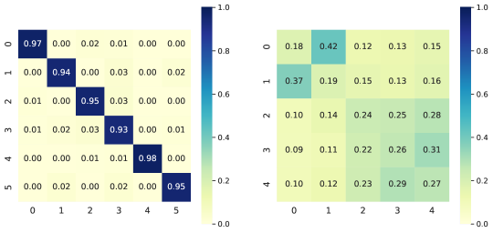
Figure 3: Compatibility matrices for the undirected version of Citeseer-Full (homophilic, left) and Chameleon (heterophilic, right).

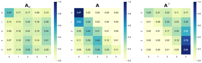
Figure 4: Weighted compatibility matrices of the undirected diffusion operator $\mathbf{A}_{u}$ and the two directed diffusion operators $\mathbf{A}$ and $\mathbf{A}^{\top}$ for Arxiv-Year. The last two have rows (classes) which are much more distinguishable then the first, despite still being heterophilic.

Appendix A Compatibility Matrices

Fig. 3 shows the compatibility matrices for both Citeseer-Full (homophilic) and Chameleon (heterophilic). Additionally,  Fig. 4 presents the weighted compatibility matrices of the undirected diffusion operator $\mathbf{A}_{u}$ and the two directed diffusion operators $\mathbf{A}$ and $\mathbf{A}^{\top}$ for Arxiv-Year. The last two have rows (classes) which are much more distinguishable then the first, despite still being heterophilic. This phenomen, called harmless heterophily, is discussed in Sec. 3.

Appendix B Harmless Heterophily Through Directions

It has been recently shown that heterophily is not necessarily harmful for GNNs, as long as nodes with the same label share similar neighborhood patterns, and different classes have distinguishable patterns [47, 48] . We find that some directed datasets, such as Arxiv-Year and Snap-Patents, show this form of harmless heterophily when treated as directed, and instead manifest harmful heterophily when made undirected (see Fig. 4 in the Appendix). This suggests that using directionality can be beneficial also when using only one layer, as we confirm empirically (see Fig. 10 in the Appendix).

Toy example. We further illustrate the concepts presented in this Section with the toy example in Fig. 5, which shows a directed graph with three classes (blue, orange, green). Despite the graph being maximally heterophilic, it presents harmless heterophily, since different classes have very different neighborhood patterns that can be observed clearly from the compatibility matrix of $\mathbf{A}$ (b). When the graph is made undirected (c), we are corrupting this information, and the classes become less distinguishable, making the task harder. We also note that both $\mathbf{A}^{\top}\mathbf{A}$ and $\mathbf{A}\mathbf{A}^{\top}$ presents perfect homophily (d), while $\mathbf{A}_{u}^{2}$ does not, in line with the discussion in previous paragraphs.

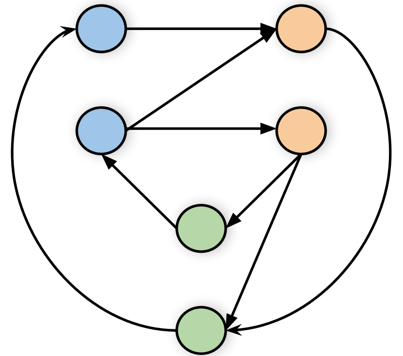
(a)

(b)

(c)

(d)

(e)

Figure 5: (a) A toy directed graph with three classes showcasing harmless heterophily. (b) Compatibility matrix of $\mathbf{A}$ showing that classes (blue, orange and green) have very different neighborhoods and can be easily distinguished. (c) Making the graph undirected makes the classes harder to distinguish, making the task harder to solve. (d) The mixed directed 2-hops ($\mathbf{A}^{\top}\mathbf{A}$ and $\mathbf{A}\mathbf{A}^{\top}$) have perfect homophily, while (e) this is not the case for the undirected 2-hop.

Appendix C Extension of Popular GNNs

We first consider an extension of GraphSAGE [4] using our Dir-GNN framework. The main choice reduces to that of normalization. In the spirit of GraphSAGE, we require the message-passing matrices $\mathbf{A}_{\leftarrow}$ and $\mathbf{A}_{\rightarrow}$ to both be row-stochastic. This is done by taking $\mathbf{A}_{\rightarrow}=\mathbf{D}_{\rightarrow}^{-1}\mathbf{A}$ and $\mathbf{A}_{\leftarrow}=\mathbf{D}_{\leftarrow}^{-1}\mathbf{A}^{\top}$, respectively. In this case, the directed version of GraphSAGE becomes

$$\mathbf{X}^{(k)}=\sigma(\mathbf{X}^{(k-1)}\mathbf{\Omega}^{(k)}+\mathbf{D}_{\rightarrow}^{-1}\mathbf{A}\mathbf{X}^{(k-1)}\mathbf{W}^{(k)}_{\rightarrow}+\mathbf{D}_{\leftarrow}^{-1}\mathbf{A}^{\top}\mathbf{X}^{(k-1)}\mathbf{W}^{(k)}_{\leftarrow}).$$

Finally, we consider the generalization of GAT [3] to the directed case. Here we simply compute attention coefficients over the in- and out-neighbours separately. If we denote the attention coefficient over the edge $(i,j)$ by $\beta_{ij}$, then the update of node $i$ at layer $k$ can be computed as

$$\mathbf{h}_{i}^{(k)}=\sigma(\sum_{(i,j)\in E}\beta_{ij}^{\rightarrow}\mathbf{W}^{(k)}_{\rightarrow}\mathbf{h}_{j}^{(k)}+\sum_{(j,i)\in E}\beta_{ji}^{\leftarrow}\mathbf{W}^{(k)}_{\leftarrow}\mathbf{h}_{j}^{(k)}),$$

where $\beta^{\rightarrow},\beta^{\leftarrow}$ are both row-stochastic matrices with support given by $\mathbf{A}$ and $\mathbf{A}^{\top}$, respectively.

Appendix D Analysis of Expressivity

In this appendix we prove the expressivity results reported in Sec. 4.1, after restating them more formally. It is important to note that we cannot build on the expressivity results from Barcelo et al. [49], since their scope is limited to undirected relational graphs, and (perhaps surprisingly) it is not possible to equivalently represent a directed graph with an undirected relational graphs, as we show in Appendix E.

We start by introducing useful concepts which will be instrumental to our discussion. As commonly done, we will assume in our analysis that all nodes have constant scalar node features $c$.

D.1 (Directed) Weisfeiler-Lehman Test

The 1-dimensional Weisfeiler-Lehman algorithm (1-WL), or color refinement, is a heuristic approach to the graph isomorphism problem, initially proposed by Weisfeiler and Leman [50]. This algorithm is essentially an iterative process of vertex labeling or coloring, aimed at identifying whether two graphs are non-isomorphic.

Starting with an identical coloring of the vertices in both graphs, the algorithm proceeds through multiple iterations. In each round, vertices with identical colors are assigned different colors if their respective sets of equally-colored neighbors are unequal in number. The algorithm continues this process until it either reaches a point where the distribution of vertices colors is different in the two graphs or converges to the same distribution. In the former case, the algorithm concludes that the graphs are not isomorphic and halts. Alternatively, the algorithm terminates with an inconclusive result: the two graphs are ‘possibly isomorphic’. It has been shown that this algorithm cannot distinguish all non-isomorphic graphs [51].

Formally, given an undirected graph $G=(V,E)$, the 1-WL algorithm calculates a node coloring $C^{(t)}:V(G)\rightarrow\mathbb{N}$ for each iteration $t>0$, as follows:

$$C^{(t)}(i)=\mathrm{RELABEL}\left(C^{(t-1)}(i),\{\mskip-6.0mu\{C^{(t-1)}(j):j\in N(i)\}\mskip-6.0mu\}\right)$$ (8)

where $\mathrm{RELABEL}$ is a function that injectively assigns a unique color, not used in previous iterations, to the pair of arguments. The function $N(i)$ represents the set of neighbours of $i$.

Since we deal with directed graphs, it is necessary to extend the 1-WL test to accommodate directed graphs. We note that a few variants have been proposed in the literature [18, 32, 52]. Here, we focus on a variant whereby in- and out-neighbours are treated separately, as discussed in [18]. This variant, which we refer to as D-WL, refines colours as follows:

$$D^{(t)}(i)=\mathrm{RELABEL}\left(D^{(t-1)}(i),\{\mskip-6.0mu\{D^{(t-1)}(j):j\in N_{\rightarrow}(i)\}\mskip-6.0mu\},\{\mskip-6.0mu\{D^{(t-1)}(j):j\in N_{\leftarrow}(i)\}\mskip-6.0mu\}\right)$$ (9)

where $N_{\rightarrow}(i)$ and $N_{\leftarrow}(i)$ are the set of out- and in-neighbors of $i$, respectively. Our first objective is to demonstrate that Dir-GNN is as expressive as D-WL. Establishing this will enable us to further show that Dir-GNN is strictly more expressive than an MPNN operating on either the directed or undirected version of a graph. Let us start by introducing some further auxiliary tools that will be used in our analysis.

D.2 Expressiveness and color refinements

A way to compare graph models (or algorithms) in their expressiveness is by contrasting their discriminative power, that is the ability they have to disambiguate between non-isomorphic graphs.

Two graphs are called isomorphic whenever there exists a graph isomorphism between the two:

Definition D.1 (Graph isomorphism).

Let $G_{1}=(V_{1},E_{1})$, $G_{2}=(V_{2},E_{2})$ be two (directed) graphs. An isomorphism between $G_{1},G_{2}$ is a bijective map $\varphi:V_{1}\rightarrow V_{2}$ which preserves adjacencies, that is: $\forall u,v\in V_{1}:(u,v)\in E_{1}\Longleftrightarrow(\varphi(u),\varphi(v))\in E_{2}$.

On the contrary, they are deemed non-isomorphic when such a bijection does not exist. A model that is able to discriminate between two non-isomorphic graphs assigns them distinct representations. This concept is extended to families of models as follows:

Definition D.2 (Graph discrimination).

Let $G=(V,E)$ be any (directed) graph and $M$ a model belonging to some family $\mathcal{M}$. Let $G_{1}$ and $G_{2}$ be two graphs. We say $M$ discriminates $G_{1}$, $G_{2}$ iff $M(G_{1})\neq M(G_{2})$. We write $G_{1}\neq_{M}G_{2}$. If there exists such a model $M\in\mathcal{M}$, then family $\mathcal{M}$ distinguishes between the two graphs and we write $G_{1}\neq_{\mathcal{M}}G_{2}$.

Families of models can be compared in their expressive power in terms of graph disambiguation:

Definition D.3 (At least as expressive).

Let $\mathcal{M}_{1},\mathcal{M}_{2}$ be two model families. We say $\mathcal{M}_{1}$ is at least as expressive as $\mathcal{M}_{2}\ \mathrm{iff}\ \forall G_{1}=(V_{1},E_{1}),G_{2}=(V_{2},E_{2}),G_{1}\neq_{\mathcal{M}_{2}}G_{2}\implies G_{1}\neq_{\mathcal{M}_{1}}G_{2}$. We write $\mathcal{M}_{1}\sqsubseteq\mathcal{M}_{2}$.

Intuitively, $\mathcal{M}_{1}$ is at least as expressive as $\mathcal{M}_{2}$ if when $\mathcal{M}_{2}$ discriminates a pair of graphs, also $\mathcal{M}_{1}$ does. Additionally, a family can be strictly more expressive than another:

Definition D.4 (Strictly more expressive).

Let $\mathcal{M}_{1},\mathcal{M}_{2}$ be two model families. We say $\mathcal{M}_{1}$ is strictly more expressive than $\mathcal{M}_{2}\ \mathrm{iff}\ \mathcal{M}_{1}\sqsubseteq\mathcal{M}_{2}\land\mathcal{M}_{2}\not\sqsubseteq\mathcal{M}_{1}$. Equivalently, $\mathcal{M}_{1}\sqsubseteq\mathcal{M}_{2}\land\exists G_{1}=(V_{1},E_{1}),G_{2}=(V_{2},E_{2}),\ \mathrm{s.t.}\ G_{1}\neq_{\mathcal{M}_{1}}G_{2}\land G_{1}=_{\mathcal{M}_{2}}G_{2}$.

Intuitively, $\mathcal{M}_{1}$ is strictly more expressive than $\mathcal{M}_{2}$ if $\mathcal{M}_{1}$ is at least as expressive as $\mathcal{M}_{2}$ and there exist pairs of graphs that $\mathcal{M}_{1}$ distinguishes but $\mathcal{M}_{1}$ does not.

Many graph algorithms and models operate by generating node colorings or representations. These can be gathered into multisets of colors that are compared to assess whether two graphs are non-isomorphic. Other than convenient, in these cases it is interesting to characterise the discriminative power at the level of nodes by means of the concept of color refinement [53, 37, 54].

Definition D.5 (Color refinement).

Let $G=(V,E)$ be a graph and $C,D$ two coloring functions. Coloring $D$ refines colouring $C$ when $\forall v,w\in V,D(v)=D(w)\implies C(v)=C(w)$.

Essentially, when $D$ refines $C$, if any two nodes are assigned the same color by $D$, the same holds for $C$. Equivalently, if two nodes are distinguished by $C$ (because they are assigned different colors), then they are also distinguished by $D$. When, for any graph, $D$ refines $C$, then we write $D\sqsubseteq C$ and, when also the opposite holds, ($C\sqsubseteq D$), we then write $D\equiv C$. As an example, for any $t\geq 0$ it can be shown that, on any graph, the coloring generated by the 1-WL algorithm at round $t+1$ refines that at round $t$, that is $C^{(t+1)}\sqsubseteq C^{(t)}$; this being essentially due to the injectivity property of the $\mathrm{RELABEL}$ function.

Importantly, as we were anticipating above, this concept can be directly translated into graph discrimination as long as graphs are represented by the multiset of their vertices’ colors, or an injection thereof. This link, which explains the use of the same symbol to refer to the concepts of color refinement and discriminative power, is explicitly shown, for example, in Bodnar et al. [55], Bevilacqua et al. [54]. More concretely, it can be shown that, if coloring $D$ refines coloring $C$, then the algorithm which generates $D$ is at least as expressive as the one generating $C$, as long as multisets of node colours are directly compared to discriminate between graphs, or they are first encoded by a multiset injection before the comparison is carried out. In the following we will resort to the concept of color refinement to prove some of our theoretical results. This approach is not only practically convenient for the required derivations, but it also informs us on the discriminative power models have at the level of nodes, something which is of relevance to us given our focus on node-classification tasks.

Furthermore, even though Dir-GNN outputs node-wise embeddings, it can be augmented with a global readout function to generate a single graph-wise embeddings $\mathbf{x}_{G}=\mathrm{READOUT}\left(\{\mskip-6.0mu\{\mathbf{x}_{i}^{(K)}:i\in V\}\mskip-6.0mu\}\right)$. We will assume that all models discussed in this section are augmented with a global readout function.

D.3 MPNNs on Directed Graphs

Before moving forward to prove our expressiveness results, let us introduce the families of architectures we compare with. These embody straightforward approaches to adapt MPNNs to directed graphs.

Let MPNN-D be a model that performs message-passing by only propagating messages in accordance with the directionality of edges. Its layers can be defined as follows:

$$\begin{split}\mathbf{m}^{(k)}_{i}&=\mathrm{AGG}^{(k)}\left(\{\mskip-6.0mu\{(\mathbf{x}_{j}^{(k-1)},\mathbf{x}_{i}^{(k-1)}):\,j\in N_{\rightarrow}(i)\}\mskip-6.0mu\}\right)\\ \mathbf{x}_{i}^{(k)}&=\mathrm{COM}^{(k)}\left(\mathbf{x}_{i}^{(k-1)},\mathbf{m}^{(k)}_{i}\right)\end{split}$$ (10)

Instead, let MPNN-U be a model which propagates messages equally along any incident edge, independent of their directionality. Its layers can be defined as follows:

$$\begin{split}\mathbf{m}^{(k)}_{i}&=\mathrm{AGG}^{(k)}\left(\{\mskip-6.0mu\{(\mathbf{x}_{j}^{(k-1)},\mathbf{x}_{i}^{(k-1)}):\,j\in N_{\rightarrow}(i)\}\mskip-6.0mu\}\cup\{\mskip-6.0mu\{(\mathbf{x}_{j}^{(k-1)},\mathbf{x}_{i}^{(k-1)}):\,j\in N_{\leftarrow}(i)\}\mskip-6.0mu\}\right)\\ \mathbf{x}_{i}^{(k)}&=\mathrm{COM}^{(k)}\left(\mathbf{x}_{i}^{(k-1)},\mathbf{m}^{(k)}_{i}\right)\end{split}$$ (11)

Note that if there are no bi-directional edges, MPNN-U is equivalent to first converting the graph to its undirected form (where the edge set is redefined as $E^{(u)}=\{(i,j):(i,j)\in E\lor(j,i)\in E\}$) and then running an undirected MPNN( Eq. 2). In practice, we observe that the number of bi-directional edges is generally small on average, while extremely small on specific datasets (see Tab. 7). In these cases, we expect the empirical performance of the two approaches to be close to each other. We remark that, in our experiments, we opt for the latter strategy as it is easier and more efficient to implement.

We can now formally define families for the models we will be comparing.

Definition D.6 (Model families).

Let $\mathcal{M}_{\mathrm{MPNN-D}}$ be the family of Message Passing Neural Networks on the directed graph (Eq. 10), $\mathcal{M}_{\mathrm{MPNN-U}}$ that of Message Passing Neural Networks on the undirected form of the graph (Eq. 11), and $\mathcal{M}_{\mathrm{Dir-GNN{}}}$ that of Dir-GNN models (Eq. 6).

D.4 Comparison with D-WL

We start by restating Theorem 4.1 more formally:

Theorem D.7.

$\mathcal{M}_{Dir-GNN{}}$ is as expressive as D-WL if $\mathrm{AGG}^{(k)}_{\rightarrow}$, $\mathrm{AGG}^{(k)}_{\leftarrow}$, and $\mathrm{COM}^{(k)}$ are injective for all $k$ and node representations are aggregated via an injective $\mathrm{READOUT}$ function.

We now prove the theorem by showing that D-WL and Dir-GNN (under the hypotheses of the theorem) are equivalent in their expressive power. We will show this in terms of color refinement and, in particular, by showing that, not only the D-WL coloring at any round $t$ refines that induced by any Dir-GNN at the same time step, but also that, when Dir-GNN’s components are injective, the opposite holds.

Proof of Theorem D.7.

Let us begin by showing that Dir-GNN is upper-bounded in expressive power by the D-WL test. We do this by showing that, at any $t\geq 0$, the D-WL coloring $D^{(t)}$ refines the coloring induced by the representations of any Dir-GNN, that is, on any graph $G=(V,E)$, $\forall v,w\in V,\quad D^{(t)}(v)=D^{(t)}(w)\implies h^{(t)}_{v}=h^{(t)}_{w}$, where $h^{(t)}_{v}$ refers to the representation of node $v$ in output from any Dir-GNN at layer $t>0$. For $t=0$ nodes are populated with a constant color: $\forall v\in V:D^{(0)}_{v}=\bar{c}$, or an appropriate encoding thereof in the case of the Dir-GNN $h^{(0)}_{v}=\textrm{enc}(\bar{c})$.

We proceed by induction. The base step trivially holds for $t=0$ given how nodes are initialised. As for the recursion step, let us assume the thesis hold for $t>0$; we seek to prove it also hold for $t+1$, showing that $\forall v,w\in V,\quad D^{(t+1)}(v)=D^{(t+1)}(w)\implies h^{(t+1)}_{v}=h^{(t+1)}_{w}$. $D^{(t+1)}(v)=D^{(t+1)}(w)$ implies the equality of the inputs of the RELABEL function given it is injective. That is: $D^{(t)}(v)=D^{(t)}(w)$, $\{\mskip-6.0mu\{D^{(t)}(u):u\in N_{\rightarrow}(v)\}\mskip-6.0mu\}=\{\mskip-6.0mu\{D^{(t)}(u):u\in N_{\rightarrow}(w)\}\mskip-6.0mu\}$, and $\{\mskip-6.0mu\{D^{(t)}(u):u\in N_{\leftarrow}(v)\}\mskip-6.0mu\}=\{\mskip-6.0mu\{D^{(t)}(u):u\in N_{\leftarrow}(w)\}\mskip-6.0mu\}$. By the induction hypothesis, we immediately get $h^{(t)}_{v}=h^{(t)}_{w}$. Also, the induction hypothesis, along with [54, Lemma 2], gives us: $\{\mskip-6.0mu\{h^{(t)}_{u}:u\in N_{\rightarrow}(v)\}\mskip-6.0mu\}=\{\mskip-6.0mu\{h^{(t)}_{u}:u\in N_{\rightarrow}(w)\}\mskip-6.0mu\}$, and $\{\mskip-6.0mu\{h^{(t)}_{u}:u\in N_{\leftarrow}(v)\}\mskip-6.0mu\}=\{\mskip-6.0mu\{h^{(t)}_{u}:u\in N_{\leftarrow}(w)\}\mskip-6.0mu\}$. Given that $h^{(t)}_{v}=h^{(t)}_{w}=\bar{h}$, we also have $\{\mskip-6.0mu\{(h^{(t)}_{u},h^{(t)}_{v}):u\in N_{\rightarrow}(v)\}\mskip-6.0mu\}=\{\mskip-6.0mu\{(h^{(t)}_{u},h^{(t)}_{w}):u\in N_{\rightarrow}(w)\}\mskip-6.0mu\}$, and $\{\mskip-6.0mu\{(h^{(t)}_{u},h^{(t)}_{v}):u\in N_{\leftarrow}(v)\}\mskip-6.0mu\}=\{\mskip-6.0mu\{(h^{(t)}_{u},h^{(t)}_{w}):u\in N_{\leftarrow}(w)\}\mskip-6.0mu\}$: it would be sufficient, for example, to construct the well-defined function $\varphi:h\mapsto(h,\bar{h})$ and invoke [54, Lemma 3]. These all represents the only inputs to a Dir-GNN layer – the two $\textrm{AGG}^{(t)}$ and the $\textrm{COM}^{(t)}$ function in particular. Being well defined functions, they must return equal outputs for equal inputs, so that $h^{(t+1)}_{v}=h^{(t+1)}_{w}$.

In a similar way, we show that, when AGG and COM functions are injective, the opposite hold, that is, $\forall v,w\in V,h^{(t)}_{v}=h^{(t)}_{w}\implies D^{(t)}(v)=D^{(t)}(w)$. The base step holds for $t=0$ for the same motivations above. Let us assume the thesis holds for $t>0$ and seek to show that for $t+1,\forall v,w\in V,h^{(t+1)}_{v}=h^{(t+1)}_{w}\implies D^{(t+1)}(v)=D^{(t+1)}(w)$. If $h^{(t+1)}_{v}=h^{(t+1)}_{w}$, then $\mathrm{COM}^{(t)}\left(\mathbf{h}_{v}^{(t)},\mathbf{m}^{(t)}_{v,\rightarrow},\mathbf{m}^{(t)}_{v,\leftarrow}\right)=\mathrm{COM}^{(t)}\left(\mathbf{h}_{w}^{(t)},\mathbf{m}^{(t)}_{w,\rightarrow},\mathbf{m}^{(t)}_{w,\leftarrow}\right)$. As $\mathrm{COM}^{(t)}$ is injective, it must also hold $\mathbf{h}_{v}^{(t)}=\mathbf{h}_{w}^{(t)}$, which, by the induction hypothesis, gives $D^{(t)}(v)=D^{(t)}(w)$. Furthermore, by the same argument, we must also have $\mathbf{m}^{(t)}_{v,\rightarrow}=\mathbf{m}^{(t)}_{w,\rightarrow}$, and $\mathbf{m}^{(t)}_{v,\leftarrow}=\mathbf{m}^{(t)}_{w,\leftarrow}$. At this point we recall that, for any node $v$, $\mathbf{m}^{(t)}_{v,\rightarrow}=\textrm{AGG}^{(t)}_{\rightarrow}(\{\mskip-6.0mu\{(h^{(t)}_{u},h^{(t)}_{v}):u\in N_{\rightarrow}(v)\}\mskip-6.0mu\})$ and $\mathbf{m}^{(t)}_{v,\leftarrow}=\textrm{AGG}^{(t)}_{\leftarrow}(\{\mskip-6.0mu\{(h^{(t)}_{u},h^{(t)}_{v}):u\in N_{\leftarrow}(v)\}\mskip-6.0mu\})$, where, by our assumption, $\textrm{AGG}^{(t)}_{\leftarrow}$, $\textrm{AGG}^{(t)}_{\rightarrow}$ are injective. This implies the equality between the multisets in input, i.e. $\{\mskip-6.0mu\{(h^{(t)}_{u},h^{(t)}_{v}):u\in N_{\rightarrow}(v)\}\mskip-6.0mu\}=\{\mskip-6.0mu\{(h^{(t)}_{u},h^{(t)}_{w}):u\in N_{\rightarrow}(w)\}\mskip-6.0mu\}$, and $\{\mskip-6.0mu\{(h^{(t)}_{u},h^{(t)}_{v}):u\in N_{\leftarrow}(v)\}\mskip-6.0mu\}=\{\mskip-6.0mu\{(h^{(t)}_{u},h^{(t)}_{w}):u\in N_{\leftarrow}(w)\}\mskip-6.0mu\}$. From these equalities it clearly follows $\{\mskip-6.0mu\{h^{(t)}_{u}:u\in N_{\rightarrow}(v)\}\mskip-6.0mu\}=\{\mskip-6.0mu\{h^{(t)}_{u}:u\in N_{\rightarrow}(w)\}\mskip-6.0mu\}$, and $\{\mskip-6.0mu\{h^{(t)}_{u}:u\in N_{\leftarrow}(v)\}\mskip-6.0mu\}=\{\mskip-6.0mu\{h^{(t)}_{u}:u\in N_{\leftarrow}(w)\}\mskip-6.0mu\}$ – one can invoke [54, Lemma 3] with the well defined function $\varphi:(h_{1},h_{2})\mapsto h_{1}$. Again, by the induction hypothesis, and [54, Lemma 2], we have $\{\mskip-6.0mu\{D^{(t)}(u):u\in N_{\leftarrow}(v)\}\mskip-6.0mu\}=\{\mskip-6.0mu\{D^{(t)}(u):u\in N_{\leftarrow}(w)\}\mskip-6.0mu\}$ and $\{\mskip-6.0mu\{D^{(t)}(u):u\in N_{\rightarrow}(v)\}\mskip-6.0mu\}=\{\mskip-6.0mu\{D^{(t)}(u):u\in N_{\rightarrow}(w)\}\mskip-6.0mu\}$. Finally, as all and only inputs to the RELABEL function are equal, $D^{(t+1)}(v)=D^{(t+1)}(w)$. The proof then terminates: as the READOUT function is assumed to be injective, having proved the refinement holds at the level of nodes, this is enough to also state that, if two graphs are distinguished by D-WL they are also distinguished by a Dir-GNN satisfying the injectivity assumptions above. ∎

As for the existence and implementation of these injective components, constructions can be found in Xu et al. [17] and Corso et al. [56]. In particular, in [17, Lemma 5], the authors show that, for a countable $\mathcal{X}$, there exist maps $f:\mathcal{X}\rightarrow\mathbb{R}^{n}$ such that function $h:X\mapsto\sum_{x\in X}f(x)$ is injective for subsets $X\subset\mathcal{X}$ of bounded cardinality, and any multiset function $g$ can be decomposed as $g(X)=\varphi\big{(}\sum_{x\in X}f(x)\big{)}$ for some function $\varphi$. As $\mathcal{X}$ is countable, there always exists an injection $Z:x\rightarrow\mathbb{N}$, and function $f$ can be constructed, for example, as $f(x)=N^{-Z(x)}$, with $N$ being the maximum (bounded) cardinality of subsets $X\subset\mathcal{X}$. These constructions are used to build multiset aggregators in the GIN architecture [17] when operating on features from a countable set and neighbourhoods of bounded size. Under the same assumptions, the same constructions can be readily adapted to express the aggregators $\text{AGG}^{(k)}_{\rightarrow},\text{AGG}^{(k)}_{\leftarrow}$ as well as READOUT in our Dir-GNN. Similarly to the above, under the same assumptions, injective maps for elements $(c,X),c\in\mathcal{X},X\subset\mathcal{X}$ can be constructed as $h(c,X)=(1+\epsilon)f(c)+\sum_{x\in X}f(x)$ for infinitely many choice of $\epsilon$, including all irrational numbers, and any function $g$ on couples $(c,X)$ can be decomposed as $g(c,X)=\varphi\big{(}(1+\epsilon)f(c)+\sum_{x\in X}f(x)\big{)}$ [17, Corollary 6]. The same approach can be extended to our use-case. In fact, for irrationals $\epsilon_{X},\epsilon_{Y}$, an injection on triple $(c,X,Y)$ (with $c\in\mathcal{X},X,Y\subset\mathcal{X}$ of bounded size and $\mathcal{X}$ countable) can be built as $h(c,X,Y)=\ell\big{(}(1+\epsilon_{X})f_{X}(c)+\sum_{x\in X}f_{X}(x),(1+\epsilon_{Y})f_{Y}(c)+\sum_{y\in Y}f_{Y}(y)\big{)}$, where $\ell$ is an injection on a countable set and $(1+\epsilon_{X})f_{X}(c)+\sum_{x\in X}f_{X}(x),(1+\epsilon_{Y})f_{Y}(c)+\sum_{y\in Y}f_{Y}(y)$ realise injections over couples $(c,X),(c,Y)$ as described above. This construction can be used to express the $\text{COM}^{(k)}$ components of Dir-GNN. In practice, in view of the Universal Approximation Theorem (UAT) [57], Xu et al. [17] propose to use Multi-Layer Perceptrons (MLPs) to learn the required components described above, functions $f$ and $\varphi$ in particular. We note that, in order to resort to the original statement of the UAT, this approach additionally requires boundedness of set $\mathcal{X}$ itself. Similar practical parameterizations can be used to build our desired Dir-GNN layers. Last, we refer readers to [56] for constructions which can be adopted in the case where initial node features have a continuous, uncountable support.

D.5 Comparison with MPNNs

In this subsection we prove Theorem 4.2, which we restate more formally and split into two separate parts, one regarding MPNN-D and the other regarding MPNN-U. We start by proving that Dir-GNN is stricly more expressive than MPNN-D, i.e an MPNN which operates on directed graphs by only propagating messages according to the directionality of edges:

Theorem D.8.

$\mathcal{M}_{\mathrm{Dir-GNN{}}}$ is strictly more powerful than $\mathcal{M}_{\mathrm{MPNN-D}}$.

We begin by first proving the following lemmas:

Lemma D.9.

$\mathcal{M}_{\mathrm{Dir-GNN{}}}$ is at least as expressive as $\mathcal{M}_{\mathrm{MPNN-D}}$ ($\mathcal{M}_{\mathrm{Dir-GNN{}}}\sqsubseteq\mathcal{M}_{\mathrm{MPNN-D}}$).

Proof of Lemma D.9.

We prove this Lemma by noting that the Dir-GNN architecture generalizes that of an MPNN-D, so that a Dir-GNN model can (learn to) simulate a standard MPNN-D by adopting particular weights. Specifically, Dir-GNN defaults to MPNN-D (which only sends messages along the out edges) if $\mathrm{COM}^{(k)}\left(\mathbf{x}_{i}^{(k-1)},\mathbf{m}^{(k)}_{i,\leftarrow},\mathbf{m}^{(k)}_{i,\rightarrow}\right)=\mathrm{COM}^{(k)}\left(\mathbf{x}_{i}^{(k-1)},\mathbf{m}^{(k)}_{i,\rightarrow}\right)$, i.e. $\mathrm{COM}$ ignores in-messages, and the two readout modules coincide. Importantly, the direct implication of the above is that whenever an MPNN-D model distinguishes two graphs, then there exists a Dir-GNN which can implement such a model and then discriminate the two graphs as well. ∎

Figure 6: Two non-isomorphic directed graphs that cannot be distinguished by any MPNN-D model but can be distinguished by Dir-GNN.

Lemma D.10.

There exist graph pairs discriminated by a Dir-GNN model which are not discriminated by any MPNN-D model.

Proof of Lemma D.10.

Let $G_{1}$ and $G_{2}$ be the non-isomorphic graphs illustrated in Fig. 6. To confirm that they are not isomorphic, simply note that node $1$ in $G_{1}$ has an in-degree of two, while no node in $G_{2}$ has an in-degree of two.

To prove that no MPNN-D model can distinguish between the two graphs, we will show that any MPNN-D induce the same coloring for the two graphs. In particular, we will show that, if $C^{(t)}(v)$ refers to the representation a MPNN-D computes for node $v$ at time step $t$, then $C^{(t)}(1)=C^{(t)}(2)=C^{(t)}(5)=C^{(t)}(6)$ and $C^{(t)}(3)=C^{(t)}(4)=C^{(t)}(7)=C^{(t)}(8)$ for any $t\geq 0$.

We proceed by induction. The base step trivially holds for $t=0$ given that nodes are all initialised with the same color. As for the inductive step, let us assume that the statement holds for $t$ and prove that it also holds for $t+1$. Assume $C^{(t)}(1)=C^{(t)}(2)=C^{(t)}(5)=C^{(t)}(6)$ and $C^{(t)}(3)=C^{(t)}(4)=C^{(t)}(7)=C^{(t)}(8)$ (induction hypothesis). Then we have:

$$C^{(t+1)}(1) =\mathrm{COM}^{(t)}\left(C^{(t)}(1),\mathrm{AGG}^{(t)}(\{\mskip-6.0mu\{\}\mskip-6.0mu\})\right)$$

$$C^{(t+1)}(2) =\mathrm{COM}^{(t)}\left(C^{(t)}(2),\mathrm{AGG}^{(t)}(\{\mskip-6.0mu\{\}\mskip-6.0mu\})\right)$$

$$C^{(t+1)}(5) =\mathrm{COM}^{(t)}\left(C^{(t)}(5),\mathrm{AGG}^{(t)}(\{\mskip-6.0mu\{\}\mskip-6.0mu\})\right)$$

$$C^{(t+1)}(6) =\mathrm{COM}^{(t)}\left(C^{(t)}(6),\mathrm{AGG}^{(t)}(\{\mskip-6.0mu\{\}\mskip-6.0mu\})\right)$$

The induction hypothesis then gives us that $C^{(t+1)}(1)=C^{(t+1)}(2)=C^{(t+1)}(5)=C^{(t+1)}(6)$. As for the other nodes, we have:

$$C^{(t+1)}(3) =\mathrm{COM}^{(t)}\left(C^{(t)}(3),\mathrm{AGG}^{(t)}(\{\mskip-6.0mu\{(C^{(t)}(3),C^{(t)}(1))\}\mskip-6.0mu\})\right)$$

$$C^{(t+1)}(4) =\mathrm{COM}^{(t)}\left(C^{(t)}(4),\mathrm{AGG}^{(t)}(\{\mskip-6.0mu\{(C^{(t)}(4),C^{(t)}(1))\}\mskip-6.0mu\})\right)$$

$$C^{(t+1)}(7) =\mathrm{COM}^{(t)}\left(C^{(t)}(7),\mathrm{AGG}^{(t)}(\{\mskip-6.0mu\{(C^{(t)}(7),C^{(t)}(5))\}\mskip-6.0mu\})\right)$$

$$C^{(t+1)}(8) =\mathrm{COM}^{(t)}\left(C^{(t)}(8),\mathrm{AGG}^{(t)}(\{\mskip-6.0mu\{(C^{(t)}(8),C^{(t)}(6))\}\mskip-6.0mu\})\right)$$

The induction hypothesis then gives us that $C^{(t+1)}(3)=C^{(t+1)}(4)=C^{(t+1)}(7)=C^{(t+1)}(8)$. Importantly, the above holds for any parameters of the $\textrm{COM}^{(t)}$ and $\textrm{AGG}^{(t)}$ functions. As any MPNN-D will always compute the same set of node representations for the two graphs, it follows that no MPNN-D can disambiguate between the two graphs, no matter the way they are aggregated. To conclude our proof, we show that there exists Dir-GNN models that can discriminate the two graphs. In view of Theorem 4.1, it is enough to show that the two graphs are disambiguated by D-WL. Applying D-WL to the two graphs leads to different colorings after two iterations (see Tab. 4), so the D-WL algorithm terminates deeming the two graphs non-isomorphic. Then, by Theorem 4.1, there exist Dir-GNNs which distinguish them. In fact, it is easy to even construct simple 1-layer architecture that can assign the two graphs distinct representations, an exercise which we leave to the reader. Importantly, note how Dir-GNN can distinguish between the two graphs hinging on the discrimination of non-isomorphic nodes such as 1, 2, something no MPNN-D is capable of doing. ∎

Iteration	Node 1	Node 2	Node 3	Node 4	Node 5	Node 6	Node 7	Node 8
1	$A$	$A$	$A$	$A$	$A$	$A$	$A$	$A$
2	$B$	$C$	$C$	$D$	$E$	$E$	$C$	$C$

$M(v)$	$\mathrm{RELABEL(M(v))}$
initialize	$A$
$(A,\{\mskip-6.0mu\{\}\mskip-6.0mu\},\{\mskip-6.0mu\{(A,A),(A,A)\}\mskip-6.0mu\})$	$B$
$(A,\{\mskip-6.0mu\{(A,A)\}\mskip-6.0mu\},\{\mskip-6.0mu\{\}\mskip-6.0mu\})$	$C$
$(A,\{\mskip-6.0mu\{\}\mskip-6.0mu\},\{\mskip-6.0mu\{\}\mskip-6.0mu\})$	$D$
$(A,\{\mskip-6.0mu\{\}\mskip-6.0mu\},\{\mskip-6.0mu\{(A,A)\}\mskip-6.0mu\})$	$E$

Table 4: Node colorings at different iterations, as well as the $\mathrm{RELABEL}$ hash function, when applying D-WL to the two graphs in Fig. 6.

With the two results above prove Theorem D.8.

Proof of Theorem D.8.

The theorem follows directly from Lemmas D.9 and D.10. ∎

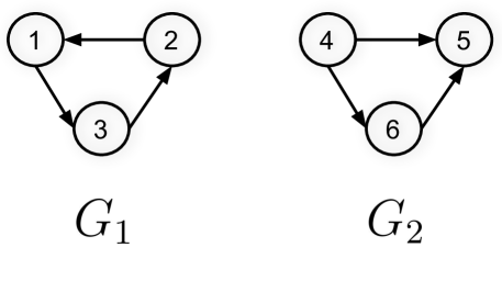
Figure 7: Two non-isomorphic directed graphs that cannot be distinguished by any MPNN-U model but can be distinguished by Dir-GNN.

Iteration	Node 1	Node 2	Node 3	Node 4	Node 5	Node 6
1	$A$	$A$	$A$	$A$	$A$	$A$
2	$B$	$B$	$B$	$C$	$B$	$D$

$M(v)$	$\mathrm{RELABEL(M(v))}$
initialize	$A$
$(A,\{\mskip-6.0mu\{(A,A)\}\mskip-6.0mu\},\{\mskip-6.0mu\{(A,A)\}\mskip-6.0mu\})$	$B$
$(A,\{\mskip-6.0mu\{(A,A),(A,A)\}\mskip-6.0mu\},\{\mskip-6.0mu\{\}\mskip-6.0mu\})$	$C$
$(A,\{\mskip-6.0mu\{\}\mskip-6.0mu\},\{\mskip-6.0mu\{(A,A),(A,A)\}\mskip-6.0mu\})$	$D$

Table 5: Node colorings at different iterations, , as well as the $\mathrm{RELABEL}$ hash function, when applying D-WL to the two graphs in Fig. 7.

Next, we focus on the comparison with MPNN-U, i.e. an MPNN on the undirected form of the graph:

Theorem D.11.

$\mathcal{M}_{\mathrm{Dir-GNN{}}}$ is strictly more expressive than $\mathcal{M}_{\mathrm{MPNN-U}}$.

Instrumental to us is to consider a variant of the 1-WL test MPNN-U can be regarded as the neural counterpart of. In the following we will show that such a variant, which we call U-WL, generates colorings which refine the ones induced by any MPNN-U and that, in turn, are refined by the D-WL test. In view of Theorem 4.1, this will be enough to show that there exists Dir-GNNs refining any MPNN-U instantiation, so that, ultimately, $\mathcal{M}_{\textrm{Dir-GNN}}\sqsubseteq\mathcal{M}_{\textrm{MPNN-U}}$.

Lemma D.12.

$\mathcal{M}_{\mathrm{Dir-GNN{}}}$ is at least as expressive as $\mathcal{M}_{\mathrm{MPNN-U}}$ ($\mathcal{M}_{\mathrm{Dir-GNN{}}}\sqsubseteq\mathcal{M}_{\mathrm{MPNN-U}}$).

Proof of Lemma D.12.

Let us start by introducing the U-WL test, which, on an undirected graph, refines node colors as:

$$A^{(t+1)}(v)=\textrm{RELABEL}\big{(}A^{(t)}(v),\{\mskip-6.0mu\{A^{(t)}(u):u\in N_{\rightarrow}(v)\}\mskip-6.0mu\}\cup\{\mskip-6.0mu\{A^{(t)}(u):u\in N_{\leftarrow}(v)\}\mskip-6.0mu\}\big{)},$$

that is, by the gathering neighbouring colors from each incident edge, independent of its direction. It is easy to show that U-WL generates a coloring that, at any round $t\geq 0$ is refined by the coloring generated by D-WL, i.e., for any graph $G=(V,E)$ it holds that $\forall v,w\in V,D^{(t)}(v)=D^{(t)}(w)\implies A^{(t)}(v)=A^{(t)}(w)$, where $D$ refers to the coloring of D-WL. Again, proceeding by induction, we have the following. First, the base step hold trivially for $t=0$. We assume the thesis holds true for $t$ and seek to show it also holds for $t+1$. If $D^{(t+1)}(v)=D^{(t+1)}(w)$ then, by the injectivity of RELABEL we must have $D^{(t)}(v)=D^{(t)}(w)$, which implies $A^{(t)}(v)=A^{(t)}(w)$ via the induction hypothesis. Additionally, we have $\{\mskip-6.0mu\{D^{(t)}(u):u\in N_{\rightarrow}(v)\}\mskip-6.0mu\}=\{\mskip-6.0mu\{D^{(t)}(u):u\in N_{\rightarrow}(w)\}\mskip-6.0mu\}$, and $\{\mskip-6.0mu\{D^{(t)}(u):u\in N_{\leftarrow}(v)\}\mskip-6.0mu\}=\{\mskip-6.0mu\{D^{(t)}(u):u\in N_{\leftarrow}(w)\}\mskip-6.0mu\}$ which, by the induction hypothesis and [54, Lemma 2], gives $\mathcal{A}^{(t)}_{\rightarrow,v}=\{\mskip-6.0mu\{A^{(t)}(u):u\in N_{\rightarrow}(v)\}\mskip-6.0mu\}=\{\mskip-6.0mu\{A^{(t)}(u):u\in N_{\rightarrow}(w)\}\mskip-6.0mu\}=\mathcal{A}^{(t)}_{\rightarrow,w}$, and $\mathcal{A}^{(t)}_{\leftarrow,v}=\{\mskip-6.0mu\{A^{(t)}(u):u\in N_{\leftarrow}(v)\}\mskip-6.0mu\}=\{\mskip-6.0mu\{A^{(t)}(u):u\in N_{\leftarrow}(w)\}\mskip-6.0mu\}=\mathcal{A}^{(t)}_{\leftarrow,w}$. From these equalities we then derive $\mathcal{A}^{(t)}_{\rightarrow,v}\cup\mathcal{A}^{(t)}_{\leftarrow,v}=\mathcal{A}^{(t)}_{\rightarrow,w}\cup\mathcal{A}^{(t)}_{\leftarrow,w}$. Indeed, let us suppose that, instead, $\mathcal{A}^{(t)}_{\rightarrow,v}\cup\mathcal{A}^{(t)}_{\leftarrow,v}\neq\mathcal{A}^{(t)}_{\rightarrow,w}\cup\mathcal{A}^{(t)}_{\leftarrow,w}$ and that, w.l.o.g., this is due by the existence of a color $\bar{a}$ such that its number of appearances in $\mathcal{A}^{(t)}_{\rightarrow,w}\cup\mathcal{A}^{(t)}_{\leftarrow,w}$ is larger than that in $\mathcal{A}^{(t)}_{\rightarrow,v}\cup\mathcal{A}^{(t)}_{\leftarrow,v}$. We write $\#^{\mathcal{A}^{(t)}_{\rightarrow,w}\cup\mathcal{A}^{(t)}_{\leftarrow,w}}(\bar{a})>\#^{\mathcal{A}^{(t)}_{\rightarrow,v}\cup\mathcal{A}^{(t)}_{\leftarrow,v}}(\bar{a})$. Then, as these are all multisets, we can rewrite $\#^{\mathcal{A}^{(t)}_{\rightarrow,w}}(\bar{a})+\#^{\mathcal{A}^{(t)}_{\leftarrow,w}}(\bar{a})>\#^{\mathcal{A}^{(t)}_{\rightarrow,v}}(\bar{a})+\#^{\mathcal{A}^{(t)}_{\leftarrow,v}}(\bar{a})$. Since $\mathcal{A}^{(t)}_{\rightarrow,w}=\mathcal{A}^{(t)}_{\rightarrow,v}$, we must have that $\#^{\mathcal{A}^{(t)}_{\rightarrow,w}}(\bar{a})=\#^{\mathcal{A}^{(t)}_{\rightarrow,v}}(\bar{a})$, which leads to necessarily having $\#^{\mathcal{A}^{(t)}_{\leftarrow,w}}(\bar{a})\neq\#^{\mathcal{A}^{(t)}_{\leftarrow,v}}(\bar{a})$. However, this entails a contradiction, because by hypothesis we had that $\mathcal{A}^{(t)}_{\leftarrow,w}=\mathcal{A}^{(t)}_{\leftarrow,v}$. Last, given that $A^{(t)}(v)=A^{(t)}(w)$, and $\mathcal{A}^{(t)}_{\rightarrow,v}\cup\mathcal{A}^{(t)}_{\leftarrow,v}=\mathcal{A}^{(t)}_{\rightarrow,w}\cup\mathcal{A}^{(t)}_{\leftarrow,w}$, being the only inputs to the RELABEL function in U-WL, then we also have that $A^{(t+1)}(v)=A^{(t+1)}(w)$, concluding the proof of the refinement.

Now, in view of Theorem 4.1, it is sufficient to show that U-WL refines the coloring induced by any MPNN-U; the lemma will then follow by transitivity. We want to show that $t\geq 0$, the U-WL coloring $A^{(t)}$ refines the coloring induced by the representations of any MPNN-U, that is, on any graph $G=(V,E)$, $\forall v,w\in V,\quad A^{(t)}(v)=A^{(t)}(w)\implies h^{(t)}_{v}=h^{(t)}_{w}$, with $h^{(t)}_{v}$ referring to the representation an MPNN-U assigns to node $v$ at time step $t$. The thesis is easily proved. It clearly holds for $t=0$ if initial node representations are produced by a well-defined function $\textrm{enc}:\bar{c}\mapsto\textrm{enc}(\bar{c})$. Then, if we assume the thesis holds for $t>0$, we can show it also holds for $t+1$. Indeed, if $A^{(t+1)}(v)=A^{(t+1)}(w)$, from the injectivity of RELABEL, it follows that $A^{(t)}(v)=A^{(t)}(w)$ and $\mathcal{A}^{(t)}_{\rightarrow,v}\cup\mathcal{A}^{(t)}_{\leftarrow,v}=\mathcal{A}^{(t)}_{\rightarrow,w}\cup\mathcal{A}^{(t)}_{\leftarrow,w}$. By the induction hypothesis, we have $h^{(t)}_{v}=h^{(t)}_{w}$ and, jointly due to [54, Lemma 2], $\{\mskip-6.0mu\{h^{(t)}_{u}:u\in N_{\rightarrow}(v)\}\mskip-6.0mu\}\cup\{\mskip-6.0mu\{h^{(t)}_{u}:u\in N_{\leftarrow}(v)\}\mskip-6.0mu\}=\{\mskip-6.0mu\{h^{(t)}_{u}:u\in N_{\rightarrow}(w)\}\mskip-6.0mu\}\cup\{\mskip-6.0mu\{h^{(t)}_{u}:u\in N_{\leftarrow}(w)\}\mskip-6.0mu\}$. Given that $h^{(t)}_{v}=h^{(t)}_{w}=\bar{h}$, it also clearly holds that $\{\mskip-6.0mu\{(h^{(t)}_{u},h^{(t)}_{v}):u\in N_{\rightarrow}(v)\}\mskip-6.0mu\}\cup\{\mskip-6.0mu\{(h^{(t)}_{u},h^{(t)}_{v}):u\in N_{\leftarrow}(v)\}\mskip-6.0mu\}=\{\mskip-6.0mu\{(h^{(t)}_{u},h^{(t)}_{w}):u\in N_{\rightarrow}(w)\}\mskip-6.0mu\}\cup\{\mskip-6.0mu\{(h^{(t)}_{u},h^{(t)}_{w}):u\in N_{\leftarrow}(w)\}\mskip-6.0mu\}$ – it is sufficient to construct the well-defined function $\varphi:h\mapsto(h,\bar{h})$ and invoke [54, Lemma 3]. These are the inputs to the well-defined functions constituting the update equations of an MPNN-U architecture, eventually entailing $h^{(t+1)}_{v}=h^{(t+1)}_{w}$. ∎

Now, with the following lemma we show that, not only $\mathcal{M}_{\mathrm{Dir-GNN{}}}$ is at least as expressive as $\mathcal{M}_{\mathrm{MPNN-U}}$, there actually exist pairs of graphs distinguished by former family but not by the latter.

Lemma D.13.

There exist graph pairs distinguished by a Dir-GNN model which are not distinguished by any MPNN-U model.

Proof of Lemma D.13.

Let $G_{1}$ and $G_{2}$ be the non-isomorphic graphs illustrated in Fig. 7. From Tab. 6 we observe that U-WL is not able to distinguish between the two graphs, as after the first iteration all nodes still have the same color: the U-WL is at convergence and terminates concluding that the two graphs are possibly isomorphic. From Lemma D.12, we conclude that no MPNN-U can distinguish between the two graphs. On the other hand, applying D-WL to the two graphs leads to different colorings after two iterations (see Tab. 5, so the D-WL algorithm terminates deeming the two graphs non-isomorphic. Then, by Theorem 4.1, there exists Dir-GNNs which distinguish them. In fact, simple Dir-GNN architectures which distinguish the two graphs are easy to construct. Importantly, we note, again, how these architectures distinguish between the two graphs by disambiguating non-isomorphic nodes such as 4, 6, something no MPNN-U is capable of doing. ∎

Last, the two results above are sufficient to prove Theorem D.11.

Proof of Theorem D.11.

The theorem follows directly from Lemmas D.12 and D.13. ∎

Iteration	Node 1	Node 2	Node 3	Node 4	Node 5	Node 6	Node 7	Node 8
1	$A$	$A$	$A$	$A$	$A$	$A$	$A$	$A$
2	$E$	$E$	$E$	$E$	$E$	$E$	$E$	$E$

$M(v)$	$\mathrm{RELABEL(M(v))}$
initialize	$A$
$(A,\{\mskip-6.0mu\{(A,A)\}\mskip-6.0mu\},\{\mskip-6.0mu\{(A,A),(A,A)\}\mskip-6.0mu\})$	$E$

Table 6: Node colorings at different iterations, as well as the $\mathrm{RELABEL}$ hash function, when applying U-WL to the two graphs in Fig. 7.

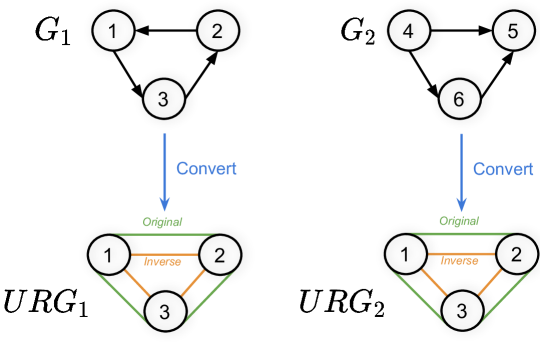
Figure 8: The two non-isomorphic directed graphs $G_{1}$ and $G_{2}$ become isomorphic when converted to an undirected relational graph. This shows that is not possible to represent directed graphs with undirected relational graphs without losing information.

Appendix E Exploring Alternative Representations for Directed Graphs

One might intuitively consider the possibility of representing a directed graph equivalently through an undirected relational graph, having two relations for original and inverse edges. However, this assumption proves to be erroneous, as illustrated by the following counterexample. Take the two non-isomorphic directed graphs illustrated in Fig. 8. Surprisingly, these two directed graphs share an identical representation as an undirected relational graph, as depicted in Fig. 8.

Kollias et al. [52] showed that it is however possible to equivalently represent a directed graph with an undirected graph having two nodes for each node in the original graph, representing the source and destination role of the node respectively.

Appendix F MPNN with Binary Edge Features

A possible alternative approach to address directed graphs involves using an MPNN [9] combined with binary edge features. In this case, the original directed graph is augmented with inverse edges, which are assigned a distinct binary feature compared to the original ones. Given the original directed graph $G=(V,E)$, we define the augmented graph as $G_{a}=(V,E_{a})$ with $E_{a}=\{((i,j),\begin{bmatrix}0\ 1\end{bmatrix}):(i,j)\in E\}\cup\{((j,i),\begin{bmatrix}1\ 0\end{bmatrix}):(i,j)\in E\}$.

An MPNN with edge features can be defined as:

$$\mathbf{m}^{(k)}_{i} =\mathrm{AGG}^{(k)}\left(\{\mskip-6.0mu\{(\mathbf{x}_{i}^{(k)},\mathbf{x}_{j}^{(k)},\mathbf{e}_{ij}):\,(i,j)\in E\}\mskip-6.0mu\}\right)$$

$$\mathbf{x}_{i}^{(k)} =\mathrm{COM}^{(k)}\left(\mathbf{x}_{i}^{(k-1)},\mathbf{m}^{(k)}_{i}\right)$$

However, since messages do not depend only on the source nodes but also on the destination node (through the edge features), this approach necessitates the materialization of explicit edge messages [58]. Given that there are $m$ such messages (one per edge) with dimension $d$, the memory complexity amounts to $\mathcal{O}(m\times d)$. This is significantly higher than the $\mathcal{O}(n\times d)$ memory complexity achieved by instantiations of Dir-GNN such as Dir-GCN or Dir-SAGE, and could lead to out-of-memory issues for even moderately sized datasets. Therefore, while having the same expressivity, our model has better memory complexity.

Appendix G Relation with Existing Methods for Directed Graphs

DGCN [25] directly employs $\mathbf{A}^{\top}\mathbf{A}$ and $\mathbf{A}\mathbf{A}^{\top}$ for spectral convolution, alongside $\mathbf{A}_{u}$. They observe that these 2-hop matrices enhance feature and label smoothness, a finding that aligns with our observations in Sec. 3. However, DGCN limits its experiments to homophilic datasets, thereby limiting the applicability of their insights. Furthermore, the model encounters several limitations: it does not provide access to directed 1-hop edges ($\mathbf{A}$ and $\mathbf{A}^{\top}$); it is constrained to the 2-hop, without the capability to access higher hops—contrastingly, our model consistently benefits from utilizing 5 or 6 layers (see Tab. 8); it is limited to a specific, GCN-like architecture, rather than a more general framework; and it lacks scalability due to the explicit computation of $\mathbf{A}^{\top}\mathbf{A}$ and $\mathbf{A}\mathbf{A}^{\top}$.

Appendix H Experimental Details

Dataset	# Nodes	# Edges	# Feat.	# C	Unidirectional Edges	Edge hom.
citeseer-full	4,230	5,358	602	6	99.61%	0.949
cora-ml	2,995	8,416	2,879	7	96.84%	0.792
ogbn-arxiv	169,343	1,166,243	128	40	99.27%	0.655
chameleon	2,277	36,101	2,325	5	85.01%	0.235
squirrel	5,201	217,073	2,089	5	90.60%	0.223
arxiv-year	169,343	1,166,243	128	40	99.27%	0.221
snap-patents	2,923,922	13,975,791	269	5	99.98%	0.218
roman-empire	22,662	44,363	300	18	65.24%	0.050

Table 7: Statistics of the datasets used in this paper.

Dataset	model_type	lr	# hidden_dim	# num_layers	jk	norm	dropout	$\alpha$
chameleon	Dir-GCN	0.005	128	5	max	True	0	1.
squirrel	Dir-GCN	0.01	128	4	max	True	0	1.
arxiv-year	Dir-GCN	0.005	256	6	cat	False	0	0.5
snap-patents	Dir-GCN	0.01	32	5	max	True	0	0.5
roman-empire	Dir-SAGE	0.01	256	5	cat	False	0.2	0.5

Table 8: Best hyperparameters for each dataset, determined through grid search, for our model.

H.1 Effective Homophily of Synthetic Graphs

For the results in Fig. 2(a), we generate directed synthetic graphs with various homophily levels using a modified preferential attachment process [59], inspired by Zhu et al. [12]. New nodes are incrementally added to the graphs until the desired number of nodes is achieved. Each node is assigned a class label, chosen uniformly at random among $C$ classes, and forms out-edges with exactly $m$ pre-existing nodes, where $m$ is a parameter of the process. The $m$ out-neighbors are sampled without replacement from a distribution that is proportional to both their in-degree and the class compatibility of the two nodes. Consequently, nodes with higher in-degree are more likely to receive new edges, leading to a "rich get richer" effect where a small number of highly connected "hub" nodes emerge. This results in the in-degree distribution of the generated graphs following a power-law, with heterophily controlled by the class compatibility matrix $\mathbf{H}$. In our experiments, we generate graphs comprising 1000 nodes and set $C=5$, $m=2$. Note that by construction, the generated graphs will not have any bidirectional edge.

H.2 Synthetic Experiment

For the results in Fig. 2(b), we construct an Erdos-Renyi graph with $5000$ nodes and edge probability of $0.001$, where each node has a scalar feature sampled uniformly at random from $[-1,1]$. The label of a node is set to 1 if the mean of the features of their in-neighbors is greater than the mean of the features of their out-neighbors, or zero otherwise.

H.3 Experimental Setup

Real-World datasets statistics are reported in table 7. All experiments are conducted on a GCP machine with 1 NVIDIA V100 GPU with 16GB of memory, apart from experiments on snap-patents which have been performed on a machine with 1 NVIDIA A100 GPU with 40GB of memory. The total GPU time required to conduct all the experiments presented in this paper is approximately two weeks. In all experiments, we use the Adam optimizer and train the model for 10000 epochs, using early stopping on the validation accuracy with a patience of 200 for all datasets apart from Chameleon and Squirrel, for which we use a patience of 400. We do not use regularization as it did not help on heterophilic datasets. For Citeseer-Full and Cora-ML we use random 50/25/25 splits, for OGBN-Arxiv we use the fixed split provided by OGB [43], for Chameleon and Squirrel we use the fixed GEOM-GCN splits [44], for Arxiv-Year and Snap-Patents we use the splits provided in Lim et al., while for Roman-Empire we use the splits from Platonov et al. [45]. We report the mean and standard deviation of the test accuracy, computed over 10 runs in all experiments.

H.4 Directionality Ablation Hyperparameters

For the ablation study in Sec. 6.2, we use the same hyperparameters for all models and datasets: $\mathrm{learning\_rate}=0.001$, $\mathrm{hidden\_dimension}=64$, $\mathrm{num\_layers}=3$, $\mathrm{norm}=True$, $\mathrm{jk}=max$. $\mathrm{norm}$ refers to applying L2 normalization after each convolutional layer, which we found to be generally useful, while $\mathrm{jk}$ refers to the type of jumping knowledge [60] used.

H.5 Comparison with State-of-the-Art Results

To obtain the results for Dir-GNN in Tab. 3, we perform a grid search over the following hyperparameters: $\mathrm{model\_type}\in\{$Dir-GCN, Dir-SAGE$\}$, $\mathrm{learning\_rate}\in\{0.01,0.005,0.001,0.0005\}$, $\mathrm{hidden\_dimensio}n\in\{32,64,128,256,512\}$, $\mathrm{num\_layers}\in\{2,3,4,5,6\}$, $\mathrm{jk}\in\{max,cat,none\}$, $\mathrm{norm}\in\{True,False\}$, $\mathrm{dropout}\in\{0,0.2,0.4,0.6,0.8,1\}$ and $\alpha\in\{0,0.5,1\}$. The best hyperparameters for each dataset are reported in table 8.

H.6 Baseline Results

GNNs for Heterophily

Results for H₂GCN, GPR-GNN and LINKX were taken from Lim et al.. Results for Gradient Gating are taken from their paper [46]. Results for FSGNN are taken from their paper [40] for Actor, Squirrel and Chameleon, whereas we re-implement it to generate results on Arxiv-year and Snap-Patents, performing the same gridsearch outlined in Sec. H.5. Results for GloGNN as well as MLP and GCN are taken from Li et al.. Results on Roman-Empire are taken from Platonov et al. [45] for GCN, H₂GCN, GPR-GNN, FSGNN and GloGNN whereas we re-implement and generate results for MLP, LINKX, ACM-GCN and Gradient Gating performing the same gridsearch outlined in Sec. H.5.

Directed GNNs

For DiGCN and MagNet, we used the classes provided by PyTorch Geometric Signed Directed library [61]. For MagNet, we tuned the $\mathrm{learning\_rate}\in\{0.01,0.005,0.001,0.0005\}$, the $\mathrm{hidden\_dim}\in\{32,64,128,256,512\}$, the $\mathrm{num\_layers}\in\{2,3,4,5,6\}$, the $K$ parameter for its chebyshev convolution to $\in\{1,2\}$, and its $q$ hyperparameter $\in\{0,0.05,0.10,0.15,0.20\}$. For DiGCN, we tune the $\mathrm{learning\_rate}\in\{0.01,0.005,0.001,0.0005\}$, the $\mathrm{hidden\_dim}\in\{32,64,128,256,512\}$, the $\mathrm{num\_layers}\in\{2,3,4,5,6\}$, and the $\alpha$ $\in\{0.05,0.10,0.15,0.20\}$.

	in_degree	out_degree	total_degree
cora_ml	41.70%	11.65%	0.00%
citeseer_full	63.45%	21.35%	0.00%
ogbn-arxiv	36.62%	10.30%	0.00%
chameleon	62.06%	0.00%	0.00%
squirrel	57.60%	0.00%	0.00%
arxiv-year	36.62%	10.30%	0.00%
snap-patents	23.38%	30.16%	6.09%
directed-roman-empire	0.00%	0.00%	0.00%

Table 9: Percentage of nodes with either in-, out- or total-degree equal to zero.

	citeseer_full	cora_ml	ogbn-arxiv	chameleon	squirrel	arxiv-year	snap-patents	roman-empire
hom.	0.949	0.792	0.655	0.235	0.223	0.221	0.218	0.050
gcn	93.37$\pm$0.22	84.37$\pm$1.52	68.39$\pm$0.01	71.12$\pm$2.28	62.71$\pm$2.27	46.28$\pm$0.39	51.02$\pm$0.07	56.23$\pm$0.37
dir-gcn($\alpha$=0.0)	93.21$\pm$0.41	84.45$\pm$1.69	23.70$\pm$0.20	29.78$\pm$1.27	33.03$\pm$0.78	50.51$\pm$0.45	51.71$\pm$0.06	42.69$\pm$0.41
dir-gcn($\alpha$=1.0)	93.44$\pm$0.59	83.81$\pm$1.44	62.93$\pm$0.21	78.77$\pm$1.72	74.43$\pm$0.74	50.52$\pm$0.09	62.24$\pm$0.04	45.52$\pm$0.14
dir-gcn($\alpha$=0.5)	92.97$\pm$0.31	84.21$\pm$2.48	66.66$\pm$0.02	72.37$\pm$1.50	67.82$\pm$1.73	59.56$\pm$0.16	71.32$\pm$0.06	74.54$\pm$0.71
sage	94.15$\pm$0.61	86.01$\pm$1.56	67.78$\pm$0.07	61.14$\pm$2.00	42.64$\pm$1.72	44.05$\pm$0.02	52.55$\pm$0.10	72.05$\pm$0.41
dir-sage($\alpha$=0.0)	94.05$\pm$0.25	85.84$\pm$2.09	52.08$\pm$0.17	48.33$\pm$2.40	35.31$\pm$0.52	47.45$\pm$0.32	52.53$\pm$0.03	76.47$\pm$0.14
dir-sage($\alpha$=1.0)	93.97$\pm$0.67	85.73$\pm$0.35	65.14$\pm$0.03	64.47$\pm$2.27	46.05$\pm$1.16	50.37$\pm$0.09	61.59$\pm$0.05	68.81$\pm$0.48
dir-sage($\alpha$=0.5)	94.14$\pm$0.65	85.81$\pm$1.18	65.06$\pm$0.28	60.22$\pm$1.16	43.29$\pm$1.04	55.76$\pm$0.10	70.26$\pm$0.14	79.10$\pm$0.19
gat	94.53$\pm$0.48	86.44$\pm$1.45	69.60$\pm$0.01	66.82$\pm$2.56	56.49$\pm$1.73	45.30$\pm$0.23	OOM	49.18$\pm$1.35
dir-gat($\alpha$=0.0)	94.48$\pm$0.52	86.13$\pm$1.58	52.57$\pm$0.05	40.44$\pm$3.11	28.28$\pm$1.02	46.01$\pm$0.06	OOM	53.58$\pm$2.51
dir-gat($\alpha$=1.0)	94.08$\pm$0.69	86.21$\pm$1.40	66.50$\pm$0.16	71.40$\pm$1.63	67.53$\pm$1.04	51.58$\pm$0.19	OOM	56.24$\pm$0.41
dir-gat($\alpha$=0.5)	94.12$\pm$0.49	86.05$\pm$1.71	66.44$\pm$0.41	55.57$\pm$1.02	37.75$\pm$1.24	54.47$\pm$0.14	OOM	72.25$\pm$0.04

Table 10: Ablation study comparing base MPNNs on the undirected graph versus their Dir-GNN extensions on the directed graph. We conducted experiments with $\alpha=0$ (only in-edges), $\alpha=1$ (only out-edges), and $\alpha=0.5$ (both in- and out-edges, but with different weight matrices). For homophilic datasets (to the left of the dashed line), incorporating directionality does not significantly enhance or may slightly impair performance. However, for heterophilic datasets (to the right of the dashed line), the inclusion of directionality substantially improves accuracy.

Appendix I Additional Results

I.1 Synthetic Experiment

We also evaluate GCN and GAT (and their Dir-GNN extensions) on the synthetic task outlined in Sec. H.2. Similarly to what observed for GraphSage (Fig. 2(b)), the Dir-GNN variant using both directions ($\alpha=0.5$) significantly outperforms the other configurations, despite not reaching 100% accuracy. The undirected models are akin to a random classifier, whereas the models using only one directions obtain between 70% and 75% of accuracy.

I.2 Ablation Study on Using Directionality

Table 10 compares using the undirected graph vs using the directed graph with our framework with different $\alpha$. We observe that only on Chameleon and Squirrel, using only one direction of the edges, in particular the out direction, performs better than using both direction. Moreover, for these two datasets, the gap between the two directions ($\alpha=0$ vs $\alpha=1$) is extremely large (more than 40% absolute accuracy). We find that this is likely due to the high number of nodes with zero in neighbors, as reported in Table 9. Chameleon and Squirrel have respectively about 62% and 57% of nodes with no in-edges: when propagating only over in edges, these nodes would get zero features. We observe a similar trend for other datasets, where $\alpha=1$ performs generally better than $\alpha=0$, in line with the fact that all these datasets have more nodes with zero in edges than out edges (Table 9). In general, using both in- and out- edges is the preferred solution.

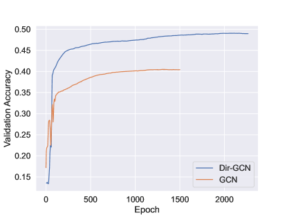
Figure 10: Performance of GCN (on the undirected version of the graph) and Dir-GCN on Arxiv-Year when using only one layer. Remarkably, directionality yields significant benefits, even in the absence of access to the homophilic directed 2-hop. This is largely attributable to the harmless heterophily exhibited by the directed graph.

I.3 Ablation Study on Using a Single Layer

In Sec. 3 we discuss how Arxiv-Year and Snap-Patents exhibit harmless heterophily when treating as directed. This suggest that even a 1-layer Dir-GNN model should be able to perform much better of its undirected counterpart, despite not being able to access the much more homophilic 2-hop. We verify this empirically by comparing a 1-layer GCN (on the undirected version of the graph) with a 1-layer Dir-GCN on Arxiv-Year. Fig. 10 presents the results, showing that Dir-GCN does indeed significantly outperform GCN.

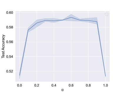
Figure 11: Dir-GNN test accuracy on Arxiv-Year for different values of the hyperparameter $\alpha$.

I.4 Ablation Study on Different Values of $\alpha$

We train Dir-GNN models on Arxiv-Year with varying values of $\alpha$, using the hyperparameters outlined in Sec. H.4. Fig. 11 presents the results: while a large drop is observed for $\alpha=0$ and $\alpha=1$, i.e. propagating messages only along one direction, the results for other values of $\alpha$ are largely similar.

I.5 Runtime Analysis

We assess the runtime of Dir-GNN by comparing it with its undirected counterpart. Specifically, in Fig. 12, we illustrate a comparison between the validation accuracies of Dir-Sage and Sage over time, measured in seconds. Both models were executed on a single NVIDIA V100 GPU with 16GB of memory. Notably, despite employing two separate weight matrices—which enhances its performance—Dir-Sage exhibits only a marginal increase in runtime. The respective runtimes per epoch are $0.71\pm 0.59$ seconds for Dir-Sage and $0.57\pm 0.48$ seconds for Sage.

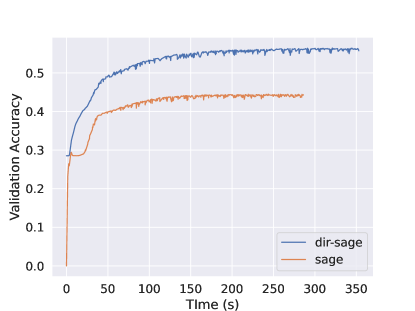
Figure 12: Validation Accuracy of Dir-Sage and Sage, displayed as a function of time (seconds).

References

- Zhou et al. [2018] Jie Zhou, Ganqu Cui, Shengding Hu, Zhengyan Zhang, Cheng Yang, Zhiyuan Liu, Lifeng Wang, Changcheng Li, and Maosong Sun. Graph neural networks: A review of methods and applications, 2018.
- Kipf and Welling [2016] Thomas N Kipf and Max Welling. Semi-supervised classification with graph convolutional networks. In ICLR, 2016.
- Veličković et al. [2017] Petar Veličković, Guillem Cucurull, Arantxa Casanova, Adriana Romero, Pietro Lio, and Yoshua Bengio. Graph attention networks. In ICLR, 2017.
- Hamilton et al. [2017] Will Hamilton, Zhitao Ying, and Jure Leskovec. Inductive representation learning on large graphs. NeurIPS, 2017.
- Shuman et al. [2013] David I Shuman, Sunil K Narang, Pascal Frossard, Antonio Ortega, and Pierre Vandergheynst. The emerging field of signal processing on graphs: Extending high-dimensional data analysis to networks and other irregular domains. IEEE Signal Processing Magazine, 2013.
- Sandryhaila and Moura [2013] Aliaksei Sandryhaila and José MF Moura. Discrete signal processing on graphs. IEEE Trans. Signal Processing, 2013.
- Bruna et al. [2014] Joan Bruna, Wojciech Zaremba, Arthur Szlam, and Yann LeCun. Spectral networks and locally connected networks on graphs. In ICLR, 2014.
- Defferrard et al. [2016] Michaël Defferrard, Xavier Bresson, and Pierre Vandergheynst. Convolutional neural networks on graphs with fast localized spectral filtering. In NeurIPS, 2016.
- Gilmer et al. [2017] Justin Gilmer, Samuel S Schoenholz, Patrick F Riley, Oriol Vinyals, and George E Dahl. Neural message passing for quantum chemistry. In ICML, 2017.
- Sen et al. [2008] Prithviraj Sen, Galileo Namata, Mustafa Bilgic, Lise Getoor, Brian Gallagher, and Tina Eliassi-Rad. Collective classification in network data. AI Magazine, 2008.
- Fey and Lenssen [2019] Matthias Fey and Jan Eric Lenssen. Fast graph representation learning with pytorch geometric, 2019.
- Zhu et al. [2020] Jiong Zhu, Yujun Yan, Lingxiao Zhao, Mark Heimann, Leman Akoglu, and Danai Koutra. Beyond homophily in graph neural networks: Current limitations and effective designs. In NeurIPS, 2020.
- Nt and Maehara [2019] Hoang Nt and Takanori Maehara. Revisiting graph neural networks: All we have is low-pass filters. arXiv, 2019.
- Altenburger and Ugander [2018] Kristen M. Altenburger and Johan Ugander. Monophily in social networks introduces similarity among friends-of-friends. Nature Human Behaviour, 2(4):284–290, April 2018. doi: 10.1038/s41562-018-0321-8. URL https://ideas.repec.org/a/nat/nathum/v2y2018i4d10.1038_s41562-018-0321-8.html.
- Lim et al. [2021] Derek Lim, Felix Matthew Hohne, Xiuyu Li, Sijia Linda Huang, Vaishnavi Gupta, Omkar Prasad Bhalerao, and Ser-Nam Lim. Large scale learning on non-homophilous graphs: New benchmarks and strong simple methods. In NeurIPS, 2021.
- Topping et al. [2022] Jake Topping, Francesco Di Giovanni, Benjamin Paul Chamberlain, Xiaowen Dong, and Michael M Bronstein. Understanding over-squashing and bottlenecks on graphs via curvature. ICLR, 2022.
- Xu et al. [2019] Keyulu Xu, Weihua Hu, Jure Leskovec, and Stefanie Jegelka. How powerful are graph neural networks? In 7th International Conference on Learning Representations, ICLR 2019, New Orleans, LA, USA, May 6-9, 2019. OpenReview.net, 2019.
- Grohe et al. [2021] Martin Grohe, Kristian Kersting, Martin Mladenov, and Pascal Schweitzer. Color refinement and its applications. In An Introduction to Lifted Probabilistic Inference. The MIT Press, 2021.
- Scarselli et al. [2009] Franco Scarselli, Marco Gori, Ah Chung Tsoi, Markus Hagenbuchner, and Gabriele Monfardini. The Graph Neural Network Model. IEEE Transactions on Neural Networks (TNN), 2009.
- Li et al. [2015] Yujia Li, Daniel Tarlow, Marc Brockschmidt, and Richard Zemel. Gated graph sequence neural networks, 2015.
- Li et al. [2016] Yujia Li, Daniel Tarlow, Marc Brockschmidt, and Richard S. Zemel. Gated graph sequence neural networks. In Yoshua Bengio and Yann LeCun, editors, 4th International Conference on Learning Representations, ICLR 2016, San Juan, Puerto Rico, May 2-4, 2016, Conference Track Proceedings, 2016. URL http://arxiv.org/abs/1511.05493.
- Vrček et al. [2022] Lovro Vrček, Xavier Bresson, Thomas Laurent, Martin Schmitz, and Mile Šikić. Learning to untangle genome assembly with graph convolutional networks. arXiv preprint arXiv:2206.00668, 2022.
- Ma et al. [2019] Yi Ma, Jianye Hao, Yaodong Yang, Han Li, Junqi Jin, and Guangyong Chen. Spectral-based graph convolutional network for directed graphs, 2019.
- Monti et al. [2018] Federico Monti, Karl Otness, and Michael M. Bronstein. Motifnet: A motif-based graph convolutional network for directed graphs. In IEEE Data Science Workshop (DSW), 2018.
- Tong et al. [2020a] Zekun Tong, Yuxuan Liang, Changsheng Sun, David S. Rosenblum, and Andrew Lim. Directed graph convolutional network. arXiv, 2020a.
- Tong et al. [2020b] Zekun Tong, Yuxuan Liang, Changsheng Sun, Xinke Li, David Rosenblum, and Andrew Lim. Digraph inception convolutional networks. In NeurIPS, 2020b.
- Zhang et al. [2021] Xitong Zhang, Yixuan He, Nathan Brugnone, Michael Perlmutter, and Matthew Hirn. Magnet: A neural network for directed graphs. In NeurIPS, 2021.
- Geisler et al. [2023] Simon Geisler, Yujia Li, Daniel J Mankowitz, Ali Taylan Cemgil, Stephan Günnemann, and Cosmin Paduraru. Transformers meet directed graphs. In Andreas Krause, Emma Brunskill, Kyunghyun Cho, Barbara Engelhardt, Sivan Sabato, and Jonathan Scarlett, editors, Proceedings of the 40th International Conference on Machine Learning, volume 202 of Proceedings of Machine Learning Research, pages 11144–11172. PMLR, 23–29 Jul 2023. URL https://proceedings.mlr.press/v202/geisler23a.html.
- Maskey et al. [2023] Sohir Maskey, Raffaele Paolino, Aras Bacho, and Gitta Kutyniok. A fractional graph laplacian approach to oversmoothing, 2023.
- Schlichtkrull et al. [2018] Michael Schlichtkrull, Thomas N. Kipf, Peter Bloem, Rianne van den Berg, Ivan Titov, and Max Welling. Modeling relational data with graph convolutional networks. In The Semantic Web. Springer International Publishing, 2018.
- Marcheggiani and Titov [2017] Diego Marcheggiani and Ivan Titov. Encoding sentences with graph convolutional networks for semantic role labeling. In Proceedings of the 2017 Conference on Empirical Methods in Natural Language Processing. Association for Computational Linguistics, 2017.
- Jaume et al. [2019] Guillaume Jaume, An-phi Nguyen, María Rodríguez Martínez, Jean-Philippe Thiran, and Maria Gabrani. edgnn: a simple and powerful GNN for directed labeled graphs. CoRR, 2019.
- Vashishth et al. [2020] Shikhar Vashishth, Soumya Sanyal, Vikram Nitin, and Partha Talukdar. Composition-based multi-relational graph convolutional networks. In International Conference on Learning Representations, 2020.
- Chien et al. [2020] Eli Chien, Jianhao Peng, Pan Li, and Olgica Milenkovic. Adaptive universal generalized pagerank graph neural network. In ICLR, 2020.
- Bo et al. [2021] Deyu Bo, Xiao Wang, Chuan Shi, and Huawei Shen. Beyond low-frequency information in graph convolutional networks. AAAI, 2021.
- Luan et al. [2022] Sitao Luan, Chenqing Hua, Qincheng Lu, Jiaqi Zhu, Mingde Zhao, Shuyuan Zhang, Xiao-Wen Chang, and Doina Precup. Revisiting heterophily for graph neural networks. In NeurIPS, 2022.
- Bodnar et al. [2022] Cristian Bodnar, Francesco Di Giovanni, Benjamin Paul Chamberlain, Pietro Liò, and Michael M Bronstein. Neural sheaf diffusion: A topological perspective on heterophily and oversmoothing in gnns. In NeurIPS, 2022.
- Di Giovanni et al. [2022] Francesco Di Giovanni, James Rowbottom, Benjamin P Chamberlain, Thomas Markovich, and Michael M Bronstein. Graph neural networks as gradient flows. arXiv, 2022.
- Abu-El-Haija et al. [2019] Sami Abu-El-Haija, Bryan Perozzi, Amol Kapoor, Nazanin Alipourfard, Kristina Lerman, Hrayr Harutyunyan, Greg Ver Steeg, and Aram Galstyan. MixHop: Higher-Order Graph Convolutional Architectures via Sparsified Neighborhood Mixing. In ICML, 2019.
- Maurya et al. [2021] Sunil Kumar Maurya, Xin Liu, and Tsuyoshi Murata. Improving graph neural networks with simple architecture design. arXiv, 2021.
- Li et al. [2022] Xiang Li, Renyu Zhu, Yao Cheng, Caihua Shan, Siqiang Luo, Dongsheng Li, and Weining Qian. Finding global homophily in graph neural networks when meeting heterophily. In ICML, 2022.
- Bojchevski and Günnemann [2018] Aleksandar Bojchevski and Stephan Günnemann. Deep gaussian embedding of graphs: Unsupervised inductive learning via ranking. In ICLR, 2018.
- Hu et al. [2020] Weihua Hu, Matthias Fey, Marinka Zitnik, Yuxiao Dong, Hongyu Ren, Bowen Liu, Michele Catasta, and Jure Leskovec. Open graph benchmark: Datasets for machine learning on graphs. In NeurIPS, 2020.
- Pei et al. [2020] Hongbin Pei, Bingzhe Wei, Kevin Chen-Chuan Chang, Yu Lei, and Bo Yang. Geom-gcn: Geometric graph convolutional networks. In ICLR, 2020.
- Platonov et al. [2023] Oleg Platonov, Denis Kuznedelev, Michael Diskin, Artem Babenko, and Liudmila Prokhorenkova. A critical look at the evaluation of GNNs under heterophily: Are we really making progress? In The Eleventh International Conference on Learning Representations, 2023.
- Rusch et al. [2023] T Konstantin Rusch, Benjamin P Chamberlain, Michael W Mahoney, Michael M Bronstein, and Siddhartha Mishra. Gradient gating for deep multi-rate learning on graphs. In ICLR, 2023.
- Ma et al. [2022] Yao Ma, Xiaorui Liu, Neil Shah, and Jiliang Tang. Is homophily a necessity for graph neural networks? In ICLR, 2022.
- Luan et al. [2023] Sitao Luan, Chenqing Hua, Minkai Xu, Qincheng Lu, Jiaqi Zhu, Xiao-Wen Chang, Jie Fu, Jure Leskovec, and Doina Precup. When do graph neural networks help with node classification: Investigating the homophily principle on node distinguishability. In NeurIPS, 2023.
- Barcelo et al. [2022] Pablo Barcelo, Mikhail Galkin, Christopher Morris, and Miguel Romero Orth. Weisfeiler and leman go relational. In The First Learning on Graphs Conference, 2022. URL https://openreview.net/forum?id=wY_IYhh6pqj.
- Weisfeiler and Leman [1968] Boris Weisfeiler and Andrei Leman. The reduction of a graph to canonical form and the algebra which appears therein. NTI Series, 1968.
- Cai et al. [1992] Jin-yi Cai, Martin Fürer, and Neil Immerman. An optimal lower bound on the number of variables for graph identifications. Combinatorica, 1992.
- Kollias et al. [2022] G. Kollias, Vasileios Kalantzis, Tsuyoshi Id’e, Aurélie C. Lozano, and Naoki Abe. Directed graph auto-encoders. In AAAI Conference on Artificial Intelligence, 2022.
- Morris et al. [2019] Christopher Morris, Martin Ritzert, Matthias Fey, William L Hamilton, Jan Eric Lenssen, Gaurav Rattan, and Martin Grohe. Weisfeiler and leman go neural: Higher-order graph neural networks. In Proceedings of the AAAI conference on artificial intelligence, 2019.
- Bevilacqua et al. [2022] Beatrice Bevilacqua, Fabrizio Frasca, Derek Lim, Balasubramaniam Srinivasan, Chen Cai, Gopinath Balamurugan, Michael M Bronstein, and Haggai Maron. Equivariant subgraph aggregation networks. In International Conference on Learning Representations (ICLR), 2022.
- Bodnar et al. [2021] Cristian Bodnar, Fabrizio Frasca, Yuguang Wang, Nina Otter, Guido F Montufar, Pietro Lió, and Michael Bronstein. Weisfeiler and lehman go topological: Message passing simplicial networks. In Proceedings of the 38th International Conference on Machine Learning. PMLR, 2021.
- Corso et al. [2020] Gabriele Corso, Luca Cavalleri, Dominique Beaini, Pietro Liò, and Petar Veličković. Principal neighbourhood aggregation for graph nets. In Advances in Neural Information Processing Systems. Curran Associates, Inc., 2020.
- Hornik et al. [1989] Kurt Hornik, Maxwell Stinchcombe, and Halbert White. Multilayer feedforward networks are universal approximators. Neural Networks, 1989.
- Tailor et al. [2022] Shyam A. Tailor, Felix Opolka, Pietro Lio, and Nicholas Donald Lane. Adaptive filters for low-latency and memory-efficient graph neural networks. In International Conference on Learning Representations, 2022.
- Barabasi and Albert [1999] Albert-Laszlo Barabasi and Reka Albert. Emergence of scaling in random networks. Science, 1999.
- Xu et al. [2018] Keyulu Xu, Chengtao Li, Yonglong Tian, Tomohiro Sonobe, Ken-ichi Kawarabayashi, and Stefanie Jegelka. Representation learning on graphs with jumping knowledge networks. In Proceedings of the 35th International Conference on Machine Learning. PMLR, 2018.
- He et al. [2022] Yixuan He, Xitong Zhang, Junjie Huang, Benedek Rozemberczki, Mihai Cucuringu, and Gesine Reinert. PyTorch Geometric Signed Directed: A Software Package on Graph Neural Networks for Signed and Directed Graphs. arXiv, 2022.