Abstract

In this note we present a fully information theoretic approach to renormalization inspired by Bayesian statistical inference, which we refer to as Bayesian Renormalization. The main insight of Bayesian Renormalization is that the Fisher metric defines a correlation length that plays the role of an emergent RG scale quantifying the distinguishability between nearby points in the space of probability distributions. This RG scale can be interpreted as a proxy for the maximum number of unique observations that can be made about a given system during a statistical inference experiment. The role of the Bayesian Renormalization scheme is subsequently to prepare an effective model for a given system up to a precision which is bounded by the aforementioned scale. In applications of Bayesian Renormalization to physical systems, the emergent information theoretic scale is naturally identified with the maximum energy that can be probed by current experimental apparatus, and thus Bayesian Renormalization coincides with ordinary renormalization. However, Bayesian Renormalization is sufficiently general to apply even in circumstances in which an immediate physical scale is absent, and thus provides an ideal approach to renormalization in data science contexts. To this end, we provide insight into how the Bayesian Renormalization scheme relates to existing methods for data compression and data generation such as the information bottleneck and the diffusion learning paradigm. We conclude by designing an explicit form of Bayesian Renormalization inspired by Wilson’s momentum shell renormalization scheme in Quantum Field Theory. We apply this Bayesian Renormalization scheme to a simple Neural Network and verify the sense in which it organizes the parameters of the model according to a hierarchy of information theoretic importance.

1 Introduction

Perhaps the central question in data science is the following: How does our understanding of a system improve as we obtain more data? The natural language for formulating this question is through statistical inference [1, 2, 3]. From the perspective of statistical inference, our understanding of a system is encoded in the probability we assign to different plausible explanations for how the system works. These explanations are formalized as probability models for observable data specified in terms of various parameters. The probability assigned to each of these models is subsequently encoded in an object called the Bayesian posterior distribution, which can be thought of as a probability distribution over all possible probability distributions for observable data. In terms of these concepts, [4] presents an answer to the aforementioned question by deriving an explicit equation governing the evolution of the posterior distribution as a function of the amount of collected data. We refer to this equation and more broadly to the idea of dynamically updating one’s beliefs in light of new data using Bayesian inference as Dynamical Bayesian Inference, or Dynamical Bayes (DB). A central observation from DB is that as new data is collected the “current” most likely model flows through the space of possible models towards the probability distribution truly responsible for generating observed data.

The idea that learning induces a flow in the space of models is immediately quite evocative of a different kind of “meta”-theory: the Renormalization Group (RG). RG is a set of ideas and strategies broadly concerned with formalizing the role of scale in our understanding and formulation of physical theories. In its original form, as conceived of by Kadanoff and Wilson [5, 6, 7], the renormalization group consists of taking a system described by a large number of degrees of freedom and performing a coarse-graining operation in which subsets of degrees of freedom are combined together and averaged over to form new collective variables. In physics applications, coarse-graining neighborhoods are determined based on considerations related to locality – that is, degrees of freedom that are nearby in physical space are joined together. For this reason, the renormalization group takes a theory which describes behaviors of a system down to arbitrarily small scales to a new theory which describes behaviors only up to a distance scale that is constrained by the size of the typical coarse graining neighborhood. In the terminology of physics, we say that a renormalization group flow takes a UV theory (a theory that is valid at arbitrarily small scales, or equivalently arbitrarily high energies) to an IR theory (a theory that is valid only at relatively large distances, or equivalently relatively low energies). From the data science perspective, one may think of an IR theory as corresponding to a naive model in which a large amount of data, namely the fine grained description of the system at length scales smaller than the prescribed cutoff, have yet to be incorporated. By contrast, a UV theory has incorporated most if not all of the available data about the system and therefore corresponds to the complete data generating model or “ground truth”. In what follows we shall often make use of this interpretation of the UV and IR. For our purposes, we will be interested in a relatively modern incarnation of renormalization that typically goes under the name of the Exact Renormalization Group (ERG) [8, 9, 10, 11, 12, 13, 14, 15, 16, 17]. ERG seeks to formalize the ideas of renormalization in a more mathematically rigorous fashion, by formulating an ERG flow as a one parameter family of theories governed by a (functional) differential equation.

Viewing a physical theory as a probability distribution for whatever observable degrees of freedom make up the system, the effect of an RG coarse-graining scheme is therefore to induce a flow through the space of possible theories – just like in DB. However, in contrast to the case of learning in which one flows through the space of models towards the data generating model, an RG flow begins at the data generating model (a UV complete theory) and flows away towards some less complete model which remains accurate only for a subset of the original degrees of freedom. This observation motivates the idea that the renormalization group flow may be regarded as a procedure “inverse” to that of dynamical Bayes, with the former taking a data generating model down to an approximate model and the latter taking an approximate model back to the data generating model. This idea was formalized in [18], in which we showed that the equation governing dynamical Bayes is formally equivalent to an Exact Renormalization Group (ERG) flow if we invert the direction of the flow. More explicitly, performing dynamical Bayes in reverse by discarding data as opposed to observing data defines an ERG scheme which we refer to as the Dynamical Bayesian Renormalization Group scheme (DB-RG) or simply Bayesian Renormalization.

In this note we aim to flesh out Bayesian Renormalization. In particular, we would like to stress how the DB-RG scheme frees renormalization from its reliance on physical locality. As we alluded to above, when performing Renormalization for physical systems one implements a coarse-graining scheme that is directly motivated by physical locality e.g. either one defines collective variables by pooling together degrees of freedom that are contained in a common spatial neighborhood, or one integrates out degrees of freedom that have support on momentum shells above a particular high energy cutoff. In either case, the existence of a hierarchy of physical scales and their role in defining the RG scheme ensures that we can interpret an ERG flow as beginning from a UV theory and ending at some IR fixed point. But what are we to do if the physical system we are interested in renormalizing has non-local interactions? Or worse yet, what if we are interested in renormalizing a model that doesn’t have a physical interpretation at all? Such a situation presents itself in recent work which seeks to import the machinery of renormalization into data science contexts as a tool for performing data compression and improving the interpretability and performance of high dimensional models [19, 20, 21, 22, 23, 24, 25, 26, 27, 28, 29].

Bayesian Renormalization overcomes the apparent lack of “real” scale by coming equipped with its own emergent scale – the distinguishability of models. Put differently, the space of models has a natural information geometric stucture [30, 31, 32] endowed by the Fisher metric, which is an infinitesimal measure of the relative entropy between a pair of probability distributions. As we will demonstrate, the DB-RG scheme automatically coarse-grains in a way that respects locality in the space of models, as dictated by the Fisher metric. This fact is particularly serendipitous in touting the utility of DB-RG for renormalizing data science models. In data compression tasks and model building considerations the Fisher metric is used to distinguish between so-called “sloppy” and “stiff” parameters. The former covary only weakly with the model output and therefore correspond to small eigenvalues of the Fisher metric, while the latter covary very strongly with the model output and therefore correspond to large eigenvalues of the Fisher metric. To hone the interpretability and generalizability of a model, one may therefore be interested in a scheme which systematically discards sloppy parameters in favor of a model that depends only on strict ones. From the perspective of the Fisher geometry, this can explicitly be thought of as a “UV regularization scheme”; a consistent method for dealing with the fact that we cannot resolve up to the arbitrarily small distances in model space necessary to identify between models that differ only along directions coordinatized by sloppy parameters [33, 34]. Thus, one way of interpreting the DB-RG scheme is as an automated data compression algorithm which sequentially integrates out “high energy” parameters (e.g. parameters associated with small eigenvalues of the Fisher metric) in the same way that a physical RG integrates out large momentum shells. In Section 4 we provide an explicit demonstration of this fact.

Putting the preceding discussion into more physical language, stiff and sloppy parameters are the data science answer to the idea of relevant and irrelevant operators. In the case where the model of interest does possess a “real” scale, this analogy becomes explicit. For example in the physics literature [35] observed that in the space of conformal field theories, the Fisher metric coincides with the Zamolodchikov metric and thus the hierarchy of relevant and irrelevant operators as dictated by the spectrum of the latter coincides with the hierarchy of stiff and sloppy parameters as dictated by the former. In a similar vein, but working in the opposite direction [36] found that the parameters that were regarded as most significant by the Information Bottleneck formalism for data compression [37] coincide with the most relevant operators in the conventional RG sense provided the model that is being compressed is given by a local statistical field theory.

In light of these observations and the information theoretic character of the emergent scale in DB-RG, another central goal of this note is to encourage the reader to think about renormalization as a manifestly information theoretic procedure. For example, consider two theories that differ only in terms of modes that exist above some observable momentum scale (ie the UV cutoff). For all intents and purposes these theories are equivalent, as there is no existing experiment which can be conducted to differentiate them. As we have now established, there is a clear analog to this in broad data science contexts: one has two models that differ only along “sloppy directions” in the model manifold. Sloppy parameters cannot be tuned except with a quantity and/or precision of observation that is not achievable due to experimental limitation. Thus, again, such models should be regarded as practically equivalent. Ultimately, this line of thinking suggests that an RG universality class should correspond to the set of all models/theories which yield equivalent predictions below a threshold set by the amount of useful information that can be collected about the system in question. From this perspective, the relevant notion of scale is always the distinguishability in model/theory space, it just happens that the same information can be communicated in terms of an energy scale in the physical case because such scales bound our experimental capability.

The organization of the paper is as follows. In Section 2.1 we review Exact Renormalization in its original physical context. We stress the perspective that a useful subclass of ERG schemes constitute functional diffusion equations, as was originally touted by [41], and recognize the role played by the physical scale in defining such diffusive ERGs. Building on the viewpoint that renormalization and diffusion are equivalent we identify diffusion as a useful device for renormalizing data models even without physical scales in Section 2.2. This picture of diffusion based renormalization for general data models is closely related to the influential diffusion learning paradigm [42] in which intractable distributions are run through diffusion channels in order to produce tractable models for data generation tasks. However, in the absence of a physical scale one cannot control the information which is coarse-grained out of the model, in contrast with physical renormalization schemes which always remove information in a hierarchy of real energy scales. This motivates the Bayesian Renormalization scheme which is introduced in Section 3. After reviewing the Fisher geometry underpinning Bayesian inference (Section 3.1), and the Dynamical Bayesian Inference scheme (Section 3.2), we explicitly derive the DB-RG scheme in Sections 3.3 and 3.4. The DB-RG scheme can be understood as a specific form of diffusive renormalization in which the information that is lost to diffusion is governed by the Fisher metric. Hence, DB-RG is a precisely the refined form of diffusion learning we sought in which the inverse of the distance measure induced by the Fisher metric plays the role of an energy scale for the purpose of the ERG. In Section 4 we illustrate the usefulness of our approach by applying the philosophy of Bayesian Renormalization to a simple autoencoder. We conclude with discussion in Section 5, in which we review our new perspective on renormalization and suggest future directions both for applications of DB-RG to data science tasks, and as a new theoretical tool.

2 Renormalization and Diffusion

In this section we review exact renormalization in its original physical context with an emphasis placed on the relationship between renormalization and diffusion. We establish that a renormalization group flow corresponds to a semigroup of conditional expectation operators acting on a sample space of random variables appropriate to a given theory. These conditional expectations generate a Markov process that can be associated with a stochastic differential equation, or equivalently with a partial differential equation of the Fokker-Planck form. The stochastic differential equation dictates a coarse-graining scheme in the usual sense, while the partial differential equation absorbs the impact of this coarse graining at the level of the probability distribution describing the variables of interest.

In a physical theory, a renormalization group flow is seeded with information about the hierarchy of momentum scales through the so-called ERG kernel, which ensures that the information coarse grained away by diffusion is associated with high energy data. By contrast, naive diffusion based renormalization discards information indiscriminately in systems that do not possess a physical scale. This motivates the Bayesian Renormalization scheme discussed in Section 3, which establishes a meaningful scale for arbitrary systems of random variables that can be seeded into the analog of the ERG kernel. This scale is associated with the distinguishability of probability distributions in the space of models/theories, and reproduces a physical scale whenever one is present.

2.1 Exact Renormalization is Diffusion

Following the lead of [41], we take the perspective that an exact renormalization group flow can be understood as a one parameter family of probability distributions, $\{P_{\Lambda}[\phi]\}_{\Lambda\in\mathbb{R}}$. Here $\Lambda$ is a physically meaningful RG scale (typically associated with a momentum cutoff), and $\phi\in\mathcal{F}$ corresponds to the field configuration relevant to a given theory. $P_{\Lambda}[\phi]$ should therefore be read as the probability density assigned to the field configuration $\phi$ at the scale $\Lambda$. Schematically, we regard

$$P_{\Lambda}[\phi]\propto e^{-S_{\Lambda}[\phi]},$$ (1)

where $S_{\Lambda}[\phi]$ is the renormalized action at scale $\Lambda$. The guiding principle of the ERG is that the flow $P_{\Lambda}[\phi]$ must be chosen in such a way that the partition function is preserved:

$$\frac{d}{d\ln\Lambda}\int_{\mathcal{F}}\mathcal{D}\phi\;P_{\Lambda}[\phi]=0.$$ (2)

The ERG principle (2) ensures that all correlation functions below the scale $\Lambda$ are preserved over the course of the ERG flow.

The most familiar form of exact renormalization is the so-called Polchinski scheme [10]. In Polchinski’s ERG, one writes the probability distribution over fields in the form

$$P_{\Lambda}[\phi]\propto e^{-\frac{1}{2}\int\frac{d^{d}p}{(2\pi)^{d}}\;\phi(p)G(p^{2})K^{-1}_{\Lambda}(p^{2})\phi(-p)}e^{-S_{int,\Lambda}[\phi]}.$$ (3)

We recognize the first term as the Gaussian distribution associated with a free field theory with propagator $G(p^{2})$, but with the incorporation of a function $K^{-1}_{\Lambda}(p^{2})$ which plays the role of a smooth cutoff function in momentum space. In words, $K_{\Lambda}^{-1}(p^{2})$ suppresses the contribution of momentum modes above the cutoff scale $\Lambda$. The second term in (3) is the exponential of the renormalized interacting action at the scale $\Lambda$.

In Polchinski’s picture, $K_{\Lambda}(p^{2})$ has a prescribed dependence on $\Lambda$, thus Polchinski’s ERG equation arises by determining the equation which must be obeyed by $S_{int,\Lambda}[\phi]$ in order to satisfy the principle (2). By a straightforward computation, one can show that the resulting equation can be put into the form:

$$\frac{d}{d\ln\Lambda}P_{\Lambda}[\phi] =\int_{M\times M}d^{d}xd^{d}y\;\left\{{C}^{Pol.}_{\Lambda}(x,y)\frac{\delta^{2}P_{\Lambda}[\phi]}{\delta\phi(x)\delta\phi(y)}+\frac{\delta}{\delta\phi(x)}\left(P_{\Lambda}[\phi]{C}^{Pol.}_{\Lambda}(x,y)\frac{\delta V^{Pol.}_{\Lambda}[\phi]}{\delta\phi(y)}\right)\right\}$$ (4)

$$\equiv\Delta P_{\Lambda}[\phi]+\text{div}\left(P_{\Lambda}[\phi]\text{grad}_{{C}^{Pol.}_{\Lambda}}V^{Pol.}_{\Lambda}[\phi]\right),$$ (5)

where

$${C}^{Pol.}_{\Lambda}(p^{2})=(2\pi)^{d}G(p^{2})^{-1}\frac{\partial K_{\Lambda}(p^{2})}{\partial\ln\Lambda};\;\;\;V^{Pol.}_{\Lambda}[\phi]=\int\frac{d^{d}p}{(2\pi)^{d}}\phi(p)G(p^{2})K^{-1}_{\Lambda}(p^{2})\phi(-p).$$ (6)

One might recognize (4) as the Fokker-Planck equation with diffusion governed by ${C}^{Pol.}_{\Lambda}(p^{2})$ and drift governed by the potential $V^{Pol.}_{\Lambda}[\phi]$. This is the first indication of a deep relationship between exact renormalization and diffusion. Note that the equivalence between (4) and (5) is just a rewriting in terms of the functional (infinite dimensional) equivalent of vector operators. This is so one can identify (4) as a functional version of Fokker-Plank.

We refer to the Polchinski approach as an ERG Scheme because it corresponds to a particular choice on how to renormalize the theory described by (3). The nexus of this choice can be traced back to the way Polchinski decided to regulate the action in (3) by introducing a smooth cutoff function $K^{-1}_{\Lambda}(p^{2})$. This choice manifests itself in the particular form of the diffusion and drift aspects of (6) specifying the Fokker-Planck equation associated with the Polchinski ERG (4). Choosing different regulating functions corresponds to different ERG schemes, and as a result different Fokker-Planck equations specified by the data (6).

More abstractly, we can define an ERG directly by specifying the data $({C}_{\Lambda},V_{\Lambda})$ corresponding to the diffusivity and drift of a Fokker-Planck equation. Equation (4) still holds but with $({C}_{\Lambda},V_{\Lambda})$ replacing ${C}^{Pol.}_{\Lambda}(p^{2}),V^{Pol.}_{\Lambda}[\phi]$. This is then an ERG corresponding to a different scheme.

The Fokker Planck equation corresponds to a bonafide ERG because it satisfies the ERG principle (2). To see that this is the case, let us now show that we can rewrite (4) in the form

$$-\frac{d}{d\ln\Lambda}P_{\Lambda}[\phi]=\int_{M}d^{d}x\;\frac{\delta}{\delta\phi(x)}\left(\Psi_{\Lambda}[\phi;x]P_{\Lambda}[\phi]\right),$$ (7)

where $M$ is the spacetime manifold on which the theory is defined [12]. Hopefully it is clear that any one parameter family $P_{\Lambda}[\phi]$ satisfying (7) also satisfies (2). This is because (7) specifies a divergence flow, that is the right hand side of (7) is a divergence in the space of field configurations. We can therefore employ the divergence theorem to observe that

$$\frac{d}{d\ln\Lambda}\int_{\mathcal{F}}\mathcal{D}\phi\;P_{\Lambda}[\phi]=-\int_{\mathcal{F}}\mathcal{D}\phi\;\int_{M}d^{d}x\;\frac{\delta}{\delta\phi(x)}\left(\Psi_{\Lambda}[\phi;x]P_{\Lambda}[\phi]\right)=0.$$ (8)

In order to write (4) in the form (7) we take

$$\Psi_{\Lambda}[\phi;x]=\int_{M}d^{d}y\;{C}_{\Lambda}(x,y)\frac{\delta\Sigma_{\Lambda}[\phi;P_{\Lambda}]}{\delta\phi(y)},$$ (9)

as has appeared previously in [17, 12, 16, 41, 45]. Here $C_{\Lambda}(x,y)$ is the ERG kernel appearing in the Fokker-Planck equation associated to the ERG, and $\Sigma_{\Lambda}[\phi;P_{\Lambda}]$ is called the scheme functional which is determined through the ERG potential $V_{\Lambda}$ via the equation

$$\Sigma_{\Lambda}[\phi;P_{\Lambda}]=-\ln\left(\frac{P_{\Lambda}[\phi]}{e^{-V_{\Lambda}[\phi]}}\right)=S_{\Lambda}[\phi]-V_{\Lambda}[\phi].$$ (10)

Plugging (9) back into (7), we reconcile (4) with the diffusion and drift aspects given by $(C_{\Lambda},V_{\Lambda})$, as desired. Together $(C_{\Lambda},V_{\Lambda})$ therefore specify a consistent scheme for regulating the high energy degrees of freedom of the field theory, in analogy with the regulating function $K^{-1}_{\Lambda}(p^{2})$ appearing in (3).

It is worth noting that (7) defines an approach to ERG that is more general than diffusion. All divergence flows, which can generically be written in the form (7), specify ERG flows as evidenced by (8). However, only the subset of divergence flows in which the reparamterization kernel $\Psi_{\Lambda}$ is taken to be of the form (9) result in Fokker-Planck equations. Equation (7) is called the Wegner-Morris equation, and ERG schemes satisfying the Wegner-Morris equation are called Wegner-Morris schemes. The choice of Wegner-Morris scheme is encapsulated entirely in the reparameterization kernel. We shall refer to reparameterization kernels which are in the form of (9) as Fokker-Planck schemes to highlight their relationship with diffusion. A Fokker-Planck scheme is specified entirely by the data $(C_{\Lambda},V_{\Lambda})$.

To conclude this section, let us briefly explore an alternative way to recognize that the Wegner-Morris equation specifies an ERG flow which allows us to supply a more concise and intuitive interpretation of the ERG. The effect of (7) on $P_{\Lambda}$ can be absorbed by continuously reparameterizing the fields $\phi$ at each new scale according to the rule

$$\phi^{\prime}(x)=\phi(x)+(\delta\ln\Lambda)\Psi[\phi;x].$$ (11)

Equation (11) should be regarded as the integral curve of $\Psi_{\Lambda}[\phi;x]$ in the space of field configurations, where we are regarding $\Psi_{\Lambda}[\phi;x]\in T\mathcal{F}$ as a tangent vector to this space. Solving (11) results in a one parameter family of field configurations $\{\phi_{\Lambda}\}_{\Lambda\in\mathbb{R}}$, in which $\phi_{\Lambda}$ can be thought of as describing the relevant field degrees of freedom at scale $\Lambda$. In this way, exact renormalization can be connected with more familiar Wilsonian renormalization schemes by interpreting equation (11) as specifying a coarse graining procedure. The coarse graining map (11) is a diffeomorphism in the space of field configurations, which means it must leave the integral

$$\int_{\mathcal{F}}\mathcal{D}\phi\;P_{\Lambda}[\phi]$$ (12)

invariant. Thus, again, we find that the equation (7) specifies a meaningful renormalization scheme in the usual sense of satisfying (2).

Specializing to Fokker-Planck ERG schemes, we can expand on this discussion. As was introduced in detail in [18], a (functional) Fokker-Planck equation of the form (4) is associated with a (functional) stochastic differential equation:

$$d\phi(x)=-\text{grad}_{{C}_{\Lambda}}V_{\Lambda}[\phi](d\ln\Lambda)+\sqrt{2}\int_{M}d^{d}y\;\sigma_{\Lambda}(x,y)dW_{\Lambda}(y).$$ (13)

Here, $W_{\Lambda}(x)$ is a function valued Weiner process, and $\sigma_{\Lambda}$ is the diffusivity kernel defined by the property that it “squares” to the covariance ${C}_{\Lambda}$:

$$\int_{M}d^{d}z\;\sigma_{\Lambda}(x,z)\sigma_{\Lambda}(z,y)={C}_{\Lambda}(x,y).$$ (14)

Equation (13) is the stochastic differential equation that arises from the deterministic gradient flow defined by (11) subject to noise with covariance governed by ${C}_{\Lambda}$. Thus, we have arrived at the punchline: An exact renormalization group flow specified by the data $(\mathcal{F},{C}_{\Lambda}(x,y),V_{\Lambda}[\phi])$ can be understood as the stochastic coarse graining of the field degrees of freedom arising from the reparameterization of the fields under the gradient of the potential $V_{\Lambda}$ subject to noise governed by ${C}_{\Lambda}$.

2.2 Diffusion is Exact Renormalization

In Section 2.1, we illustrated how exact renormalization group flows a la Wegner-Morris correspond to a subclass of functional diffusion equations (7). These Fokker-Planck schemes are specified by the pair $({C}_{\Lambda},V_{\Lambda})$ which set, respectively, the diffusion and drift of a stochastic process underyling the Fokker-Planck equation associated with the ERG. The stochastic process (13) explicitly describes a coarse graining of the field degrees of freedom, while the related diffusion equation encodes the impact of such a coarse graining on the renormalized action, resulting in an effective field theory at each scale. One of the main insights of [18] is that viewing exact renormalization as a diffusion process suggests an approach to renormalization which is applicable to a wider class of systems modeled by probability distributions, beyond merely those which posses a physical interpretation. In this section we will outline this approach.

Consider a random variable $Y$ with sample space $S$. For simplicity, let us assume that $Y$ is a continuous random variable, and $S$ is a Riemannian manifold. A general class of diffusion equations on $S$ are then specified by a one parameter family of probability distributions $\{p_{t}(y)\}_{t\in\mathbb{R}}$ along with a metric $g_{t}:TS\times TS\rightarrow\mathbb{R}$ and a potential function $V_{t}:S\rightarrow\mathbb{R}$ such that

$$\frac{dp_{t}(y)}{dt}=\Delta p_{t}(y)+\text{div}\left(p_{t}(y)\text{grad}_{g_{t}}V_{t}(y)\right).$$ (15)

Equation (15) is the Fokker-Planck equation associated with the stochastic differential equation

$$dY^{i}_{t}=-\left(\text{grad}_{g_{t}}V_{t}\right)^{i}dt+\sqrt{2}(\theta_{t})^{i}_{j}dW^{j}_{t}$$ (16)

where

$$\delta^{kl}(\theta_{t})^{i}_{k}(\theta_{t})^{j}_{l}=g_{t}^{ij}.$$ (17)

It is worth noting here that the $g_{t}$ plays a double role. From one perspective it is the metric in this process but interpreted in terms of the underlying statistics it is the inverse of the covariance matrix. Then equations (15) and (16) should be compared with (4) and (13) from the exact renormalization context.

As was the case in Section 2.1, we can formally solve for the gradient flow of the potential $V_{t}$ to determine a one parameter family of renormalized degrees of freedom. To be precise, let $\gamma:\mathbb{R}\rightarrow S$ be a one parameter family of points in $S$ solving the gradient flow problem

$$\frac{d\gamma_{t}}{dt}=\text{grad}_{g_{t}}V\rvert_{\gamma_{\tau}}.$$ (18)

In terms of $\gamma_{t}$ we can now write (16) in the form

$$dY^{i}_{t}=-\dot{\gamma_{t}}^{i}dt+\sqrt{2}(\theta_{t})^{i}_{j}dW^{j}_{t}.$$ (19)

where $\dot{\gamma}_{t}$ and $\theta_{t}$ correspond to the drift and diffusion, respectively.

The Fokker-Planck equation (15) has a schematic solution:

$$p_{t}(y)=\int_{S}d^{d}y_{0}\;\pi(y,y_{0};t)p_{0}(y_{0}).$$ (20)

Here, $p_{0}(y)$ is the initial data, and $\pi(y,y_{0};t)$ is the Heat Kernel. Provided the drift and diffusion are constant over the full sample space the diffusion kernel will be a Gaussian of the form

$$\pi(y,y_{0};t)=\mathcal{N}(\gamma_{t},tg_{t}^{-1})(y-y_{0})$$ (21)

Explicitly, $\pi(y,y_{0};t)$ is the transition probability density for a sample point to start from $y_{0}$ and diffuse to $y$ in a time $t$. We shall interpret the heat kernel as a stochastic map encoding the implicit coarse graining scheme associated with the diffusive RG flow.

This picture of renormalization is closely related to information theoretic approaches to renormalization from the high energy physics community that have been employed in the study of holography and operator algebras [46, 47, 48]. To see this, note that we can encode (20) as a semigroup of conditional expectation operators acting on the space of functions on $S$, $E_{t}:\Omega^{0}(S)\rightarrow\Omega^{0}(S)$. The conditional expectation operator $E_{t}$ acts as

$$E_{t}(f)=\mathbb{E}_{\pi_{t}}(f(Y_{0}))=\int_{S}\text{Vol}_{S}(y_{0})\;\pi(y,y_{0};t)f(y_{0}),$$ (22)

so that, for example, the posterior predictive distribution is given by

$$p_{t}(y)=E_{t}(p_{0})(y)=\mathbb{E}_{\pi_{t}}(p_{0}(Y_{0})).$$ (23)

The set of operators $\{E_{t}\}_{t\in\mathbb{R}}$ form a semigroup in the sense that

$$E_{t_{2}}\circ E_{t_{1}}=E_{t_{1}+t_{2}}.$$ (24)

In a more general context, a conditional expectation on a von Neumann algebra $M$ is a projection of $M$ to a subset $N\subset M$, $E:M\rightarrow N$, which retains the normalization of states such that $E(\mathbb{1}_{M})=\mathbb{1}_{N}$ [49]. A very broad class of renormalization schemes accessible to quantum probabilities can subsequently be formulated as a semigroup of conditional expectation operators $\{E_{\Lambda}\}_{\Lambda\in\mathbb{R}}$ acting on the space of operators affiliated with a given system. In a recent work [48], this form of renormalization was given the name code subspace renormalization to reflects its relationship with error correction.

The relationship between renormalization and diffusion is very satisfying because we can think of a diffusion process as destroying some of the fine grained information stored in a very complicated, “UV complete” probability distribution. Indeed, this is the point of view which is advocated for in the influential diffusion learning paradigm [42]. In diffusion learning, one begins with a highly complex and intractable distribution $p_{0}$ which is run through a forward diffusion process for a time $t_{f}$ in order to arrive at an analytic distribution, $p_{f}$. One can then sample data from $p_{0}$ by first sampling data from $p_{f}$ and subsequently solving a “reverse” stochastic differential equation derived from (16) [53]. To be more precise, given a generic forward diffusion process specified by the SDE

$$dY_{t}^{i}=\mu^{i}_{t}(Y_{t})dt+\sigma_{t}{}^{i}{}_{j}(Y_{t})dW_{t}^{j},$$ (25)

the associated reverse SDE is of the form [54]

$$dY_{s}^{i}=\bigg{\{}\mu^{i}_{s}-\frac{1}{2}\partial_{j}\bigg{(}\delta^{kl}\sigma_{s}{}^{i}{}_{k}\sigma_{s}{}^{j}{}_{l}\bigg{)}-\delta^{kl}\sigma_{s}{}^{i}{}_{k}\sigma_{s}{}^{j}{}_{l}\partial_{j}\ln p_{s}\bigg{\}}\bigg{\rvert}_{Y_{s}}ds+\sigma_{s}{}^{i}{}_{j}(Y_{s})dW_{s}^{j}$$ (26)

Here, $t$, which runs from $0$ to $t_{f}$, is the forward time, while $s$, which runs from $t_{f}$ to the initial time $0$, is the reverse time. The reverse SDE is determined by all of the same data as the forward SDE with exception of the score functions – $\partial_{j}\ln p_{s}(y)$. Here, $p_{s}(y)$ is probability distribution obtained by diffusing $p_{0}$ according to the forward SDE up to the reverse time $s$. Simulating the reverse SDE therefore amounts to efficiently reconstructing the scores. In the machine learning community, a resolution to this problem has been presented in terms of the training of a score based generative algorithm (see [53] for a comprehensive review). Interestingly, such a score-based model can be interpreted as a statistical inference problem in which the distribution $p_{s}$ is learned by observing draws from intermediate diffused distributions. We will revisit this in Section 3 where we provide an alternative point of view on the same fact by demonstrating that inverting a diffusion process can be thought of as a Bayesian inference experiment.

Based on the observations of the preceding paragraph, one may be tempted to say that diffusion learning can be thought of as a form of exact renormalization for data science models. In light of the correspondence between ERG and diffusion, such a statement is technically correct. However, naive diffusion lacks a very crucial feature which is at the core of a good renormalization group flow; namely a meaningful notion of scale. Indeed, unlike physical renormalization which coarse grains hierarchically over length/energy scales, naive diffusion removes information in an essentially unstructured way. Thus, while basic diffusion can technically be regarded as a form of renormalization, it fails to provide real control over how a probability model changes as a function of any meaningful scale. More plainly, in physics based renormalization we know that the information lost to coarse graining correspond to high energy modes via the construction of the ERG kernel. By contrast, naive diffusion of a probability distribution apparently discards information indiscriminately. Ultimately, this is problem that the Bayesian approach to diffusion/renormalization will overcome.

3 Bayesian Renormalization and Information Geometry

We now turn to an information theoretic approach to renormalization which will provide a meaningful scale that is applicable to arbitrary random variables, and reproduces the physical scale when the chosen random variable descends from a physical system. This notion of scale is defined in terms of the Fisher information metric, and therefore corresponds to the distinguishability between points in the space of probability distributions. Our new approach emphasizes the role of information and information geometry in renormalization, which we now understand broadly as a mechanism for identifying equivalence classes of probability distributions that are indistinguishable as predictive models at a level of precision fixed by the amount of accessible data. This viewpoint allows us to draw a very sharp analogy between renormalization and aspects of data compression [55, 56, 57, 58, 36], data generation [59, 60, 61], data classification [62, 63, 64, 65, 66, 67, 40], dimensional reduction and model selection [68, 33, 34] commonly studied in data science and machine learning. We present this approach to renormalization through its relationship with Bayesian inference to highlight its information theoretic origin.

Bayesian inference is an approach to reconstructing the probability distribution responsible for generating a sequence of observed data. Let $Y$ be a random variable taking values in the sample space $S$. Given a series of independent draws, $\{y_{t}\}_{t=1}^{T}$, from the data generating distribution $p^{*}_{Y}$, the output of a Bayesian inference is a posterior predictive distribution, $p_{T}(y)$, which is the best approximation to $p^{*}_{Y}$ given the data that has been observed. The idea of Bayesian renormalization is to perform Bayesian inference in reverse by discarding data rather than incorporating it. The posterior predictive distribution subsequently pools attributes from models that are similar but not equivalent to the data generating model. As we shall illustrate, this defines an RG scheme that automatically encodes an information theoretic notion of relevant and irrelevant degrees of freedom. It is specified by an explicit diffusion process that enforces the relevance criterion by coarse-graining in a way that sequentially “integrates out” parameters in order of their relevance just like one would sequentially integrate over momentum shells in a Wilsonian renormalization.

3.1 Bayesian Inference and Information Geometry

The first step in Bayesian inference is model selection. This corresponds to choosing a parametric family of probability distributions on $S$, $p_{Y\mid\Theta}(y\mid\theta)$. A priori, we should consider any allowed distribution for $Y$ as a candidate for the data generating distribution. Thus, we might take

$$p_{Y\mid\Theta}(y\mid\theta)=e^{-\theta^{i}S_{i}(y)}$$ (27)

where here $\{S_{j}(y)\}_{j\in\mathcal{J}}$ is the set of log-likelihoods corresponding to allowed probability models for $Y$. In principle the space of models might be infinite dimensional, however for simplicity let us assume that it is finite.

Let $\mathcal{M}=\{p_{Y\mid\Theta}(y\mid\theta)\;|\;\theta\in\mathbb{R}^{n}\}$. In words, $\mathcal{M}$ is a space whose points correspond to probability distributions for $Y$. By construction, this space has a local coordinate system given in terms of the parameters $\theta$. A natural basis for the tangent space of $\mathcal{M}$, is given to us in terms of the score vectors $\underline{\ell}_{i}=\frac{\partial}{\partial\theta^{i}}\ln(p_{Y\mid\Theta}(y\mid\theta))$. It is easy to see that these vectors are linearly independent and spanning insofar as they are isomorphic to the coordinate basis $\underline{\partial}_{i}$. Moreover, when viewed as functions on $S$ the score vectors have zero expectation value due to the normalization condition on $p$:

$$\mathbb{E}_{\theta}(\underline{\ell}_{i}(Y))=\int_{S}d^{d}y\;p_{Y\mid\Theta}(y\mid\theta)\frac{\partial\ln(p_{Y\mid\Theta}(y\mid\theta))}{\partial\theta^{i}}=\frac{\partial}{\partial\theta^{i}}\int_{S}d^{d}y\;p_{Y\mid\Theta}(y\mid\theta)=0.$$ (28)

In terms of this basis, we define the Fisher information matrix:

$$\mathcal{I}_{ij}(\theta)=\mathbb{E}_{\theta}(\underline{\ell}_{i}\underline{\ell}_{j})=\mathbb{E}_{\theta}\left(\frac{\partial\ln(p_{Y\mid\Theta}(Y\mid\theta))}{\partial\theta^{i}}\frac{\partial\ln(p_{Y\mid\Theta}(Y\mid\theta))}{\partial\theta^{j}}\right).$$ (29)

The Fisher matrix (29) should be interpreted as the components of a metric, the Fisher metric, on $\mathcal{M}$ in the basis $\{\underline{\ell}_{i}\}$.

The Fisher metric provides an infinitesimal measure of the similarity between two models in $\mathcal{M}$. This can be seen most clearly through the relationship between the Fisher metric and the KL-divergence. Recall,

$$D_{KL}(\theta\parallel\theta^{\prime})=\mathbb{E}_{\theta}\left(\ln(\frac{p_{Y\mid\Theta}(Y\mid\theta)}{p_{Y\mid\Theta}(Y\mid\theta^{\prime})})\right).$$ (30)

measures the relative entropy between two distributions. $D_{KL}$ is an information divergence, which means that $D_{KL}(\theta\parallel\theta^{\prime})\geq 0$ and it is equal to zero if and only if $\theta=\theta^{\prime}$. This makes $D_{KL}$ a good measure of the distinguishability between models. In general, however, $D_{KL}$ is not a symmetric function of $\theta$ and $\theta^{\prime}$ and therefore cannot be regarded itself as an inner product. Nonetheless, in the immediate neighborhood of a point $\theta\in\mathcal{M}$ the KL-divergence can be expanded to quadratic order as

$$D_{KL}(\theta\parallel\theta^{\prime})=\frac{1}{2}\mathcal{I}_{ij}(\theta)\delta\theta^{i}\delta\theta^{j}+\mathcal{O}(\delta\theta^{3}).$$ (31)

The Fisher metric plays a significant role in parameter estimation because it encodes the sensitivity of a model’s output to changes in parameter values [40]. This is closely related to the task of distinguishing between model parameters that are “sloppy” and “stiff” [69, 70]. Strict parameters covary strongly with the model output and therefore correspond to large eigenvalues of the Fisher metric. Sloppy parameters, on the other hand, covary only weakly with the model output and therefore correspond to small eigenvalues of the Fisher metric. From a geometric perspective, this means that we can think of sloppy directions – that is directions coordinatized by sloppy parameters – as being highly compact in the space of models. In particular, two models that differ only along sloppy directions will be very hard to distinguish. As a consequence, sloppy parameters require an extensive amount or quality of observed data in order to be fit [71]. However, because these parameters only weakly impact the predictive power of the model it may also be possible to systematically remove them in favor of a reduced model that depends only a sufficient set of strict parameters.

This state of affairs strongly resembles the typical use case of the renormalization group in physical theories. Our ability to meaningfully distinguish between theories is capped by our capacity to perform experiments which measure physics beyond particular scales. In this sense, two theories which yield equivalent predictions except beyond scales that cannot be experimentally probed must be regarded as practically equivalent. If we view a physical theory as parameterized by the Fourier modes of field degrees of freedom, it is precisely the high energy modes which correspond to the “sloppy parameters” since one requires an extensive or even impossible set of measurements to distinguish between theories that differ only at very high energy scales. From this point of view, we recognize renormalization as a scheme for systematically regulating sloppy model parameters in order to arrive at an equivalence class of models that cannot be distinguished at the level of accuracy admitted by our present ability to observe data.

In recent work [34] it has been suggested that a similar approach would be very useful in a more broad data science context. Quite serendipitously, this can be thought of as a “UV regularization scheme” from the perspective of the Fisher geometry – it is a consistent method for dealing with the fact that we cannot resolve up to the arbitrarily small distances in model space necessary to identify between models that differ along directions coordinatized by sloppy parameters. As we introduce the Bayesian renormalization scheme, we will highlight how it automatically performs an information geometrically natural regularization to this end, that is oriented directly towards intelligently removing these sloppy degrees of freedom.

3.2 Dynamical Bayesian Inference

The upshot of Section 3.1 is that the starting point of a Bayesian inference experiment can be understood as the specification of a Riemannian information geometry $(\mathcal{M},\mathcal{I})$, where $\mathcal{M}$ consists of all possible probability models for $Y$, and $\mathcal{I}$ is an infinitesimal measure of the distinguishability between models. As we have discussed, adopting an information geometric approach to Bayesian inference already allows us to begin formulating the correspondence between learning in the space of models and renormalization. The next step in Bayesian inference is updating, which we regard as a specification of dynamics in the space of models.

In conventional Bayesian inference, the updating phase starts by specifying a prior distribution $\pi_{0}:\mathcal{M}\rightarrow\mathbb{R}$ which acts as the initial data for the dynamical system. In light of observed data, the prior distribution is updated to the posterior distribution, $\pi_{T}(\theta)$, by using Bayes’ law. That is

$$\pi_{T}(\theta)\propto\left(\prod_{t=1}^{T}p_{Y\mid\Theta}(y_{t}\mid\theta)\right)\pi_{0}(\theta).$$ (32)

The constant of proportionality can be deduced by enforcing that $\pi_{T}$ be a normalized probability distribution on $\mathcal{M}$. One should interpret (32) as specifying that the probability the data generating model lives in a small neighborhood of the point $\theta\in\mathcal{M}$ is proportional to the probability that one would have observed the existing sample conditional on the underlying parameter value being in such a neighborhood, multiplied by the prior weight given to that neighborhood. In this way the posterior distribution is slowly trained around the region in model space where the data generating distribution lives.

In [4], we asked the question of what Bayesian inference would look like as a continuous time dynamical system. In other words, we think of data as being continuously observed so that the sample $\{y_{t}\}_{t=1}^{T}$ is growing as a function of the “time” parameter $T$. We subsequently showed that the posterior distribution is governed by an integro-differential equation

$$\frac{\partial\pi_{T}(\theta)}{\partial T}=-\left(D_{KL}(\theta^{*}\parallel\theta)-\mathbb{E}_{\pi_{T}}\left(D_{KL}(\theta_{*}\parallel\Theta)\right)\right)\pi_{T}(\theta).$$ (33)

Here $\theta_{*}$ is the parameter corresponding to the location of the data generating distribution in $\mathcal{M}$, and we have assumed that this value is unique. The equation (33) has a schematic solution

$$\pi_{T}(\theta)\propto e^{-TD_{KL}(\theta_{*}\parallel\theta)}$$ (34)

which we interpret as a Bolzmann distribution with “energy” given by the KL-divergence between the data generating model and a model at $\theta\in\mathcal{M}$. This observation is intimately related with the idea of treating the distinguishability of models as a kind of “energy” scale.

At sufficiently late $T$ the posterior distribution will be of the form

$$\pi_{T}(\theta)=\mathcal{N}(\mu_{T},\frac{1}{T}\mathcal{I}(\mu_{T})^{-1})(\theta).$$ (35)

Here $\mu_{T}$ is the $T$-path of the maximum a posterior (MAP) estimate. We regard the specification of $\mu_{T}$ as defining a new dynamical element. Once the full time path of the MAP has been observed, one can construct a potential function $V:\mathcal{M}\rightarrow\mathbb{R}$ for which $\mu_{T}$ is defined to be a gradient flow

$$\frac{d}{dT}\mu_{T}=\text{grad}_{\mathcal{I}}V\rvert_{\mu_{T}}.$$ (36)

One can consider $V$ as encoding the details of the sequence with which data was observed in relation to the sequential evolution of the answer to the question of which single model best approximates the data generating distribution. Eventually, as $T\rightarrow\infty$ we expect that $\mu_{T}\rightarrow\theta_{*}$.

One may interpret (35) as specifying that the posterior distribution $\pi_{T}$ is localized around the MAP, $\mu_{T}$, with a characteristic width given by $\frac{1}{T}\mathcal{I}(\mu_{T})^{-1}$. Notice, the width of this distribution is shrinking as a function of $T$. In other words, as more and more data is observed, the posterior trains around a smaller and smaller neighborhood of the MAP. This means that the posterior predictive model at time $T$ will become more and more precisely attuned to the specific characteristics of the data generating distribution.

We conclude that a dynamical Bayesian inference scheme is specified by the triple $(\mathcal{M},\mathcal{I},V)$, where $\mathcal{M}$ specified the set of allowed models, $\mathcal{I}$ endows this set with a notion of scale in terms of the distinguishability of nearby models, and $V$ encodes the sequence with which data is observed and the trajectory of the MAP as it converges towards the data generating model. This set of data is cosmetically very similar to the data defining an exact renormalization group flow, $(\mathcal{F},{C}_{\Lambda},V_{\Lambda})$. We will now demonstrate how one can define an information theoretic exact renormalization group flow in terms of the dynamical Bayesian inference scheme.

3.3 Backward Inference and Model Space Renormalization

The posterior predictive distribution is obtained by taking the convolution of the posterior and the likelihood model:

$$p_{T}(y)=\mathbb{E}_{\pi_{T}}\left(p_{Y\mid\Theta}(y\mid\Theta)\right)=\int_{\mathcal{M}}\text{Vol}_{\mathcal{M}}(\theta)\pi_{T}(\theta)p_{Y\mid\Theta}(y\mid\theta).$$ (37)

Taking the posterior to be of the form (35), we can see that (37) is a weighted sum of probability models for $Y$ in which the set of models outside a small neighborhood of the MAP are heavily suppressed. Notice that the posterior distribution is playing a very similar role to the cutoff function in (3), only in the opposite direction. The smooth cutoff suppresses high momentum modes or, in other words, information at short scales. Conversely, as $T$ increases, the posterior distribution suppresses information at large distances as measured by the information geometry on $\mathcal{M}$. This makes sense, as we have dictated renormalization is a form of diffusion in which information is removed from the probability model. By contrast, Bayesian inference incorporates new information with the observation of each new data point. This discrepancy motivates the idea of considering Bayesian inference in reverse in which, rather than incorporating new data, an experimenter sequentially removes data from the reconstructed model. We refer to this process as backward inference.

Formally, backward inference corresponds to flowing along the inverse “time” parameter $\tau=\frac{1}{T}$. In terms of this parameter,

$$\pi_{\tau}(\theta)=\mathcal{N}(\mu_{\tau},\tau\mathcal{I}(\mu_{\tau})^{-1})(\theta).$$ (38)

As $\tau$ increases the width of the posterior distribution increases and a larger set of models are meaningfully incorporated into the posterior predictive distribution. Over time the set of models which live in a small neighborhood of the data generating model will receive less and less weight in the posterior predictive distribution, as the reconstructed model becomes a weighted sum of a more diverse set of models. Inputting (38) into (37), we find the $\tau$-dependent predictive distribution:

$$p_{\tau}(y)=\int_{\mathcal{M}}\text{Vol}_{\mathcal{M}}(\theta)\;\mathcal{N}(\mu_{\tau},\tau\mathcal{I}(\mu_{\tau})^{-1})(\theta)p_{Y\mid\Theta}(y\mid\theta),$$ (39)

which defines a semigroup of conditional expectation values acting in the space of models. Hence we regard (39) as defining a renormalization group flow directly in the space of models.

3.4 Bayesian Inversion and Data Space Renormalization

Operationally, (39) defines a perfectly reasonable renormalization scheme which coarse grains in model space. However, there is utility to translating (39) so that it can also be understood as explicitly coarse graining in the space of data realizations, as is more standard in typical renormalization schemes. To accomplish this task, we will restrict our attention to spaces of models that are realized in the context of Bayesian inversion [72].

The goal of a Bayesian inversion problem is to deduce the signal, $\theta$, that predicated a measured output or data, $y$. The data and signal are related by a map, $y=G(\theta)$, which we regard as a deterministic model. In practice, either due to explicit stocasticity or limitations to measurement precision, we must regard the realized output as a random variable which depends conditionally on the signal as

$$Y\mid\Theta=G(\Theta)+N$$ (40)

where $N$ is a random variable that is conditionally independent of $Y$ and encodes the aforementioned noise. One may therefore read (40) as dictating that $Y$ and $\Theta$ are related by a “law” $Y=G(\Theta)$ but subject to some random fluctuations governed by $N$. Provided that the noise is distributed with some density $p_{N}(n)$, we can form the conditional density of $Y$ given $\Theta$ by pulling this measure back by (40) to obtain

$$p_{Y\mid\Theta}(y\mid\theta)=p_{N}(y-G(\theta)).$$ (41)

The procedure described above is familiar from conventional approaches to Bayesian inference for modeling complex systems and constructing neural networks. For example, in the most simple case of a feed-forward neural network, the deterministic function $G(\theta)$ is given by $f(x;W,b)$ where $f$ is the neural network architecture specified by its set of weights, $W$, and biases, $b$. In the simplest case of $L^{2}$ loss, we take

$$p_{Y\mid\Theta}(y\mid\theta)=\mathcal{N}(0,\sigma^{2})(y-G(\theta))$$ (42)

where $\sigma^{2}$ is a hyperparameter that sets a scale for the tolerated prediction error.

Given a parametric family of probability distributions for $Y$ which can be written in the form (41), we are motivated to rewrite the posterior predictive distribution (39) as an integral over $S$ by forming the pushforward measure via the mapping $G$.

$$p_{\tau}(y)=\int_{S}\text{Vol}_{S}(y_{0})\;\mathcal{N}(\gamma_{\tau},\tau K_{\tau}^{-1})(y-y_{0})\;p_{N}(y_{0}).$$ (43)

Here $\gamma_{\tau}=G(\mu_{\tau})$ is the data prediction associated with the maximum a posteriori estimate, and

$$(K_{\tau}^{-1})^{ab}=\frac{\partial G^{a}}{\partial\theta^{i}}\frac{\partial G^{b}}{\partial\theta^{j}}\mathcal{I}^{ij}_{\tau}$$ (44)

is the pushforward of the inverse Fisher metric by the map $G$ to give the induced Fisher metric on the data space itself.

We can now compare (43) with (20) and recognize that the posterior distribution, when pushed forward into the sample space by the map $G$, is the heat kernel of an associated convection-diffusion equation. In particular, (43) can be read as the solution to a Fokker-Planck equation

$$\frac{dp_{\tau}}{d\tau}=\Delta p_{\tau}+\text{div}\left(p_{\tau}\text{grad}_{K_{\tau}}V_{\tau}\right)$$ (45)

or equivalently, as describing a stochastic process

$$dY^{a}_{\tau}=-\left(\text{grad}_{K_{\tau}}V_{\tau}\right)^{a}d\tau+\sqrt{2}(\theta_{\tau})^{a}_{b}dW^{b}_{\tau}.$$ (46)

As discussed in (36), $V_{\tau}$ is a potential function on the sample space for which $\gamma_{\tau}$ is a gradient flow, and $\delta^{cd}(\theta_{\tau})^{a}_{c}(\theta_{\tau})^{b}_{d}=(K^{-1}_{\tau})^{ab}$.

Equations (43), (45), and (46) complete an explicit mapping between a dynamical Bayesian inference scheme and an exact renormalization group flow which we can now represent schematically as the identification:

$$(\mathcal{M},\mathcal{I},V)\leftrightarrow(S,K,V).$$ (47)

The mapping (47) provides a novel information theoretic interpretation for exact renormalization as the inverse process dual to a Bayesian inference procedure governed by (33). In particular, we have realized our goal of demonstrating how performing the inverse of statistical inference, that is by discarding data rather than collecting data, implements an information theoretic renormalization scheme with emergent scale given by the distinguishability of probability distributions in model space. The role of this scale in coarse graining can be seen through the relationship between the ERG kernel, $K^{-1}_{\tau}$, and the Fisher information metric.

3.5 Comparison with Diffusion Learning

For clarity, it is helpful to compare the governing equations of Bayesian Renormalization and Dynamical Bayes with the forward and reverse diffusion processes introduced in Section 2.2. From the diffusion learning perspective, one begins by running the data generating distribution through a forward diffusion process specified by an SDE of the form (25). This results in a more tractable distribution which can subsequently be used to generate samples from the data generating distribution by appealing to the associated reverse SDE (26). To accomplish this step one must implement an algorithm which reconstructs the score functions; a task which can be formulated as a Bayesian learning problem. By contrast, our derivation of the Bayesian Renormalization scheme has ensued in exactly the opposite direction. We began with a Bayesian learning problem governed by the dynamical Bayesian inference equation (33). Then, we constructed the reverse process (relative to Bayes) by studying how the learned distribution changes when data is removed as opposed to incorporated. The result was a diffusion process governed by the SDE (46).

One should identify the forward diffusion, (25), with the Bayesian diffusion process, (46). Similarly, one should identify the reverse diffusion process, (26), with the Dynamical Bayesian learning process, (33). In summary, one way of interpreting Bayesian renormalization is as an information theoretic formulation of the observation that the reverse SDE associated with a diffusion process corresponds with a statistical learning problem. The advantage of this approach is that, opposed to a naive diffusion scheme as would be implemented by (20), the Bayesian diffusion scheme intelligently discards information according to a hierarchy of importance as dictated by the Fisher metric. In this respect we hope that Bayesian Renormalization can inspire new approaches to information theoretic optimal diffusion learning while also providing insights into the underlying information theoretic character of both diffusion learning and generic renormalization.

To this end, although we have introduced Bayesian Renormalization through its relationship with Bayesian inference, we should stress that it motivates a methodology that can be undertaken without the need to first perform a Bayesian inference experiment. In particular, we can renormalize a family of probability distributions by diffusing it through the space of possible models with the diffusion kernel $\mathcal{N}(\gamma_{\tau},\tau K^{-1}_{\tau})$; one can understand this procedure as information theoretic form of diffusion learning where Eqn. (46) provides an explicit proposal for a forward diffusion process which coarse grains information in a hierarchy of importance as specified by the Fisher metric. In turn, the reverse SDE associated with (46) through the identification (26) has an explicit interpretation as encoding the Bayesian learning of the data generating distribution in the time $T$ corresponding to the reintegration of removed data. Here, $K^{-1}_{\tau}$ should be chosen by first computing the Fisher information matrix of the model space of interest, and subsequently pushing this matrix forward in the sample space by selecting a function $G:\mathcal{M}\rightarrow S$. The potential function $V_{\tau}$ can be chosen arbitrarily, and will govern the mean tendency of the diffusion process. Thus, the Bayesian renormalization scheme corresponds to the choices of $G$ and $V_{\tau}$, with $\mathcal{I}$ being fixed by the system. This is significant because $\mathcal{I}$ is what encodes the information theoretic scale of the problem.

The identification of the mapping $G$ should be thought of as a form of data compression in which a deterministic model for the data realizations in terms of the parameters is postulated. Over the course of the Bayesian renormalization, there will be a flowing in these parameters resulting in the formulation of an effective model. This procedure is related to a variety of different data compression techniques such as the information bottleneck [37] and variational autoencoding [56]. In this way, the Bayesian Renormalization scheme makes direct contact with previous insights into the relationship between model building/dimensional reduction for complex systems and the renormalization group such as [21, 19, 20, 36].

4 Implementation of Bayesian Renormalization

The preceding discussion has been largely abstract. Thus, in this penultimate section, we shall provide some insight into the overarching themes of our work through an explicit example. Rather than analyzing a Bayesian inference experiment, we apply the philosophy of Bayesian Renormalization directly to a Neural Network in order to stress the general applicability of our approach. In particular, we will demonstrate how Bayesian Renormalization can be used to systematically remove “sloppy” parameters from a autoencoder network.

Machine learner’s approach	Bayesian’s approach
Neural Network	Statistical Model
Weights $w_{i}$ and biases $b_{i}$	Model parameter $\theta_{i}$
Training Sample	Observed Data
Trained weights/biases	Parameter terminal distribution $\theta^{*}$
Minimization of loss function	Maximization of log-likelihood $\ln p_{Y|\Theta}(y|\theta)$

Table 1: Approximate dictionary mapping equivalent quantities in Bayesian statistics to those in the study of neural networks.

Before delving into our experiment, it is instructive to reflect on the relationship between Bayesian inference and Machine Learning. To quote [73], “Statisticians and computer scientists often use different language for the same thing.” In this regard, it is helpful to provide a brief dictionary outlining the correspondence between Bayesian inference and the study of neural networks which can be found in Table 1. For a more extensive review of how Bayesian statistics is related to neural networks, see [74].

4.1 Autoencoders

An autoencoder is a type of (artificial) neural network trained using unsupervised learning which is used to create efficient encodings of a set of unlabelled input data. By definition, autoencoders are composed of two blocks: an encoder and a decoder; typically both blocks are trained simultaneously.

Assuming the encoded and decoded message spaces are Euclidean, let

$$\chi =\mathbb{R}^{n} \tilde{\chi} =\mathbb{R}^{m}.$$ (48)

where $n$ denotes the dimension of the input data, and $m$ the dimension of the latent space chosen when the network is initialized. For each data instance $y\in\chi$, we denote the encoded latent space representation as $\tilde{y}\in\tilde{\chi}$. Let $E_{\theta}$ be the encoder function, parameterized by a set of variables $\{\theta_{i}\}$ and mapping from the space of decoded (source) messages $\chi$ to the space of encoded messages $\tilde{\chi}$,

$$E_{\theta}:\chi\to\tilde{\chi}.$$ (49)

Similarly, $D_{\phi}$ is the decoding function, parameterized by a second set of variables $\{\phi_{j}\}$ and mapping from the space of encoded messages $\tilde{\chi}$ to the space of decoded messages $\chi$,

$$D_{\phi}:\tilde{\chi}\to\chi.$$ (50)

As a choice of autoencoder architecture, we consider a simple dense, (linear) multi-layer perceptron network with no biases, $n$ input neurons, and $m$ latent space neurons (where the number of output neurons is thus constrained also to $n$). Selecting the architecture as a multi-layer perceptron network is intentional: since each node is fully connected with an associated weight parameter, one may expect the network to have many weights that covary comparatively weakly with the output of the network. A schematic summary of the network architecture is presented in Figure 1.

Figure 1: Highly degenerate model architecture with $n=4,m=2$. A simple MLP autoencoder with a pair of linear (dense) layers.

In the case of the aforementioned network, we choose the element-wise encoder and decoder layers to be

$$(E_{\theta})_{i} =\alpha_{\text{Enc}}(\theta_{ij}x^{j}) (D_{\phi})_{j} =\alpha_{\text{Dec}}(\phi_{ij}x^{j}),$$ (51)

where $\alpha_{\text{Enc}},\alpha_{\text{Dec}}$ are the encoder and decoder activation functions. Each parameter of the encoder and decoder networks are elements of the corresponding weight matrix $\theta_{ij}$ – the machine learner may be more familiar with the usual form $\alpha(Wx+b)$ where $W$ is the typical weight matrix and $b$ is the corresponding bias vector. For all activations, we choose the Rectified Linear Unit (ReLU) activation defined as

$$\alpha(x)=\max(0,x):=\begin{cases}x\text{ if }x>0\\ 0\text{ otherwise}\end{cases}$$ (52)

Let $D\subset\chi$ denote the set of training data. Upon the introduction of each new item of training data, $y\in D$, the parameters of the autoencoder are updated to minimize a given loss function $L(y\mid\theta,\phi)$. In the following numerical examples, we consider the typical mean squared error (MSE) loss defined by

$$L(y\mid\theta,\phi)=\frac{1}{n}\sum_{j=1}^{n}(y_{j}-D_{\phi}E_{\theta}(y)_{j})^{2}.$$ (53)

4.2 Information Shell Renormalization Scheme

In the course of this note, we have stressed that a crucial question in any data science context is how we can arrive at an effective model for a given system using only the most relevant set of parameters. Indeed, it is typical for models to possess parameters that are comparatively less sensitive than others, and we have argued that these can be identified systematically via the Fisher matrix. As we have stressed in Table 1 a Neural Network, like our autoencoder, can be understood as a family of statistical models quantified in terms of the various parameters used to initialize its architecture. In our case, each set of parameters $(\theta,\phi)$ corresponds to a different autoencoder, with our best estimate of the “true” or optimal autoencoder given by the value of these parameters which is realized after all of the training data have been utilized. We denote these optimal parameters by $(\theta^{*},\phi^{*})$. Appealing again to Table 1, we can give a more decidedly probabilistic viewpoint on the family of autoencoders by regarding each autoencoder $(\theta,\phi)$ as initializing a probability distribution over data of the form

$$p_{Y\mid\Theta,\Phi}(y\mid\theta,\phi)\propto\text{exp}\bigg{(}-L(y\mid\theta,\phi)\bigg{)}.$$ (54)

Then, the minimization of the loss can equivalently be regarded as a maximization of the log-likelihood specified in (54).

Regarding the set of all possible autoencoders as a family of statistical models, we can employ the machinery developed in Section 3.1 to endow this space with an information geometry. In particular, the Fisher matrix of the encoder layer may be calculated explicitly from the trained model using the approach outlined in [75]. During this analysis the trained parameters of the decoder are left untouched – this allows comparison between pruning methods while eliminating inter-layer interactions. We denote by $\mathcal{I}_{ij}$ the components of the resulting Fisher matrix. Because it is computed after training one should regard this as the Fisher metric evaluated at the point $(\theta^{*},\phi^{*})$.

As we have discussed, the eigenvalues of the Fisher metric serve as a proxy for the relevance of the various parameters which are included in the model class. From a physical perspective, one may think of each parameter $\theta_{i}$ as a mode of a particular theory, and of its associated diagonal element in the Fisher metric $\mathcal{I}_{ii}$ as corresponding to its characteristic “length scale”. Parameters with small Fisher diagonals vary weakly under the acquisition of new data and therefore require either extremely fine measurements or very large amounts of data in order to substantiate even an incremental change in their trained value. For this reason, we can think of these parameters as changing only on very fine length scales in the space of models. Conversely, parameters with larger Fisher values vary strongly with the model and therefore possess features that can be distinguished more broadly with less or less fine-tuned data.

In light of these observations, we now propose the most simple-minded form of Bayesian renormalization. We introduce a sliding parameter, $\Lambda$, and divide the set of parameters into two subsets:

$$\Theta^{>}_{\Lambda}\equiv\{\theta_{i}\;|\;\mathcal{I}_{ii}>\Lambda\},\qquad\Theta^{<}_{\Lambda}\equiv\{\theta_{i}\;|\;\mathcal{I}_{ii}\leq\Lambda\}.$$ (55)

The set $\Theta^{>}_{\Lambda}$ consists of those parameters that covary with the model output on “length” scales greater than $\Lambda$. We refer to these parameters equivalently as relevant/stiff parameters relative to the scale $\Lambda$ for obvious reasons. Conversely, the set $\Theta^{<}_{\Lambda}$ consists of those parameters that covary with the model output on “length” scales below $\Lambda$. We refer to these parameters equivalently as irrelevant/sloppy relative to the scale $\Lambda$. The renormalization procedure we shall consider is simply to remove the parameters in $\Theta^{<}_{\Lambda}$. This realizes a reduced/renormalized model that depends only on the parameters $\Theta^{>}_{\Lambda}$. One should think of this as akin to a hard cutoff regularization scheme in a Quantum Field Theory in which modes that depend on physics at length scales smaller than a given cutoff $\Lambda$ are systematically removed.

4.3 Experimental results

Model property	Value
Input (Output) dimension	$784$
Latent space dimension	$20$
Number of encoder parameters (pre-prune)	$15680$
Mean diagonal Fisher value	$0.7148$
Optimizer	ADAM
ADAM $(\alpha,\beta_{1},\beta_{2},\epsilon)$	$(0.001,0.9,0.999,10^{-8})$
Cutoff $\Lambda$	$(0,0.125,0.25,...,2.375)$

Table 2: Values of configurable properties of the autoencoder network.

For our experiment, we begin by training the autoencoder described in Section 4.1 on the MNIST dataset. Recall that MNIST is a series of approximately 50 thousand training samples and 10 thousand testing samples consisting of $28\times 28$ pixel (784 dimensional) images depicting handwritten digits 0 through 9. The network and optimizer settings are outlined in Table 2.

After having trained the model, we perform the Bayesian renormalization scheme outlined above. The result of this procedure at various values of the cutoff parameter $\Lambda$ can be seen in Figure 3. To illustrate the sense in which the Bayesian RG scheme more adequately coarse grains the model with respect to the information contained in its various parameters we have also provided two alternative schemes. In the first scheme, demonstrated in Figure 4, the same number of parameters are removed in each iteration as in the Fisher-inspired scheme, but using a uniform distribution over the parameters of the model. The second alternative scheme is a popular form of pruning for neural networks which we refer to as “magnitude inspired pruning”. In the magnitude inspired approach a fixed number of parameters are removed in each iteration corresponding to the remaining parameters with the smallest absolute value, hence the name.

As one can see in Figure 3, the autoencoder remains remarkably effective even once more than half of its parameters have been removed, provided these parameters are removed using the Bayesian scheme. To understand this result it is instructive to look at the distribution of (diagonal) Fisher elements associated with the encoder – see Figure 5. Here one can see that there is a large gap in the spectrum at $\Lambda\sim 0.1$ – we regard this gap as identifying the genuinely “sloppy” parameters in the model. In Figure 2 we explore the loss landscape as a function of the number of removed parameters, comparing the Fisher-motivated scheme with random parameter removal and magnitude inspired pruning. In regards to this comparison there are two important points to be made. Firstly, the Fisher-motivated scheme produces minimal losses up to the aforementioned cutoff at $\Lambda\sim 0.1$. Shortly thereafter, the losses of the Fisher motivated pruning scheme exceed those of the magnitude scheme. This is expected; for $\Lambda>0.1$ the Fisher scheme begins to remove parameters that are relevant to the performance of the model. The loss responds strongly to the removal of these paramters. In other words, Figure 2 demonstrates that the Fisher scheme effectively distinguishes both irrelevant and relevant parameters.

A different way of understanding the preceding discussion serves to contextualize the relationship between RG and statistical learning. One can imaging performing the pruning procedure in reverse, whereby one incorporates new paramters one at a time in order to improve the model’s performance. From this perspective, Figure 2 demonstrates that the Fisher scheme most rapidly reaches minimal losses among the three approaches here considered.

One can summarize the preceding discussion by observing the distinctive shape of the loss curve produced by the Fisher pruning scheme. Up to the aforementioned “scale” of $\Lambda\sim 0.1$ the loss is essentially stable to the pruning of parameters. Thereafter, the removal of subsequent parameters results in noticeable decreases in the performance of the model. The result is a ‘hockey-stick’ shaped curve: for $\Lambda\lesssim 0.1$ the pruning removes irrelevant parameters that covary weakly with the output of the model, and thus only marginally affect the loss; likewise for $\Lambda>0.1$ the pruning begins to remove ‘relevant’ parameters that covary heavily with the output of the model. In other words, the Bayesian RG scheme has identified a characteristic “scale” in the model and has dictated that the inclusion of parameters which are irrelevant with respect to that scale may be excluded from the model without any change in performance – this is precisely the goal of an RG flow. It is instructive to recognize that the notion of scale which is relevant in this instantiation of RG has a direct relationship with the number of parameters included in the model.

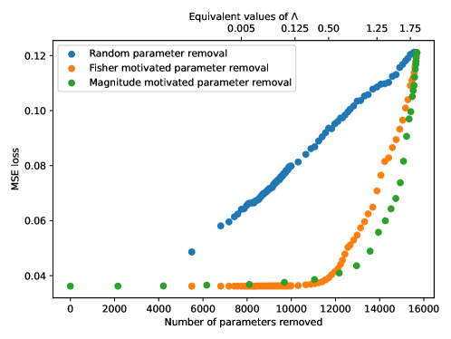
Figure 2: Mean square error loss between the true distribution and output of the pruned networks.

(a) Source images. Input to autoencoder.

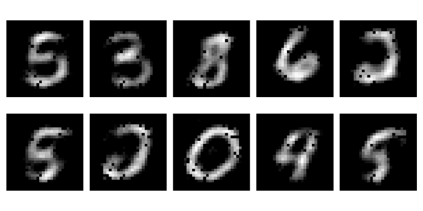
(b) Cutoff $\Lambda=0$. 15680 parameters. Unpruned autoencoder.

(c) Cutoff $\Lambda=0.125$. 10168 parameters removed (64.8%).

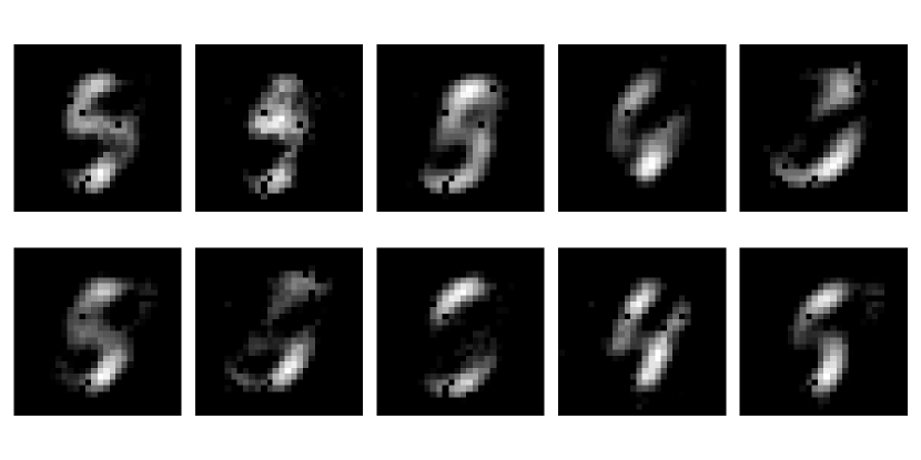
(d) Cutoff $\Lambda=1.25$. 13879 parameters removed (82.1%).

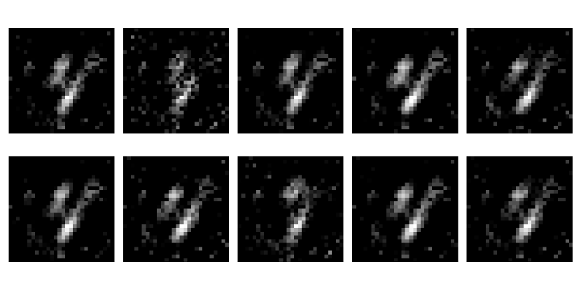
(e) Cutoff $\Lambda=1.75$. 15386 parameters removed (98.1%).

(f) Cutoff $\Lambda=2.375$. All (15680) parameters removed (100%).

Figure 3: Fisher-motivated pruning with variable cutoffs $\Lambda$.

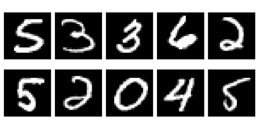
(a) Source images. Input to autoencoder.

(b) 15680 parameters. Unpruned autoencoder. Equivalent to cutoff $\Lambda=0$.

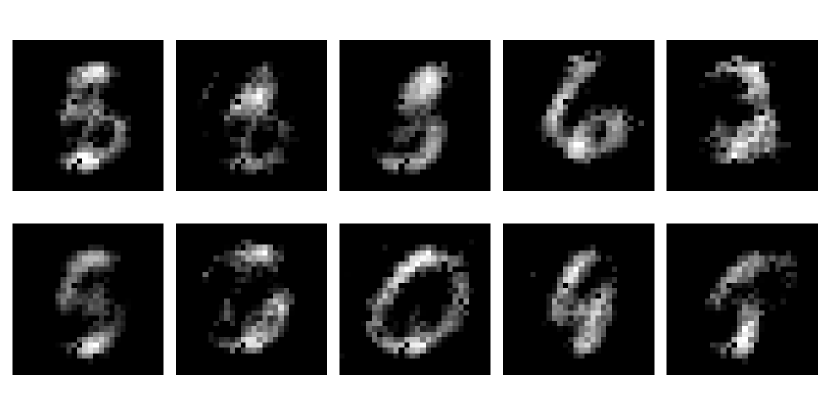
(c) 10168 parameters removed (64.8%). Equivalent to cutoff $\Lambda=0.125$.

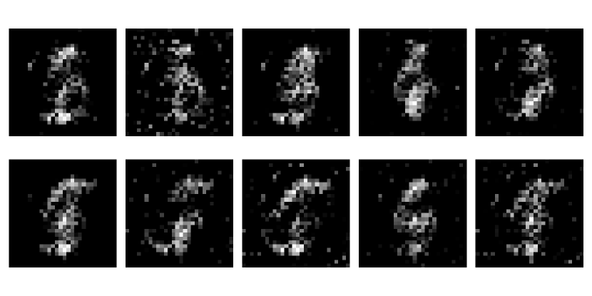
(d) 13879 parameters removed (82.1%). Equivalent to cutoff $\Lambda=1.25$.

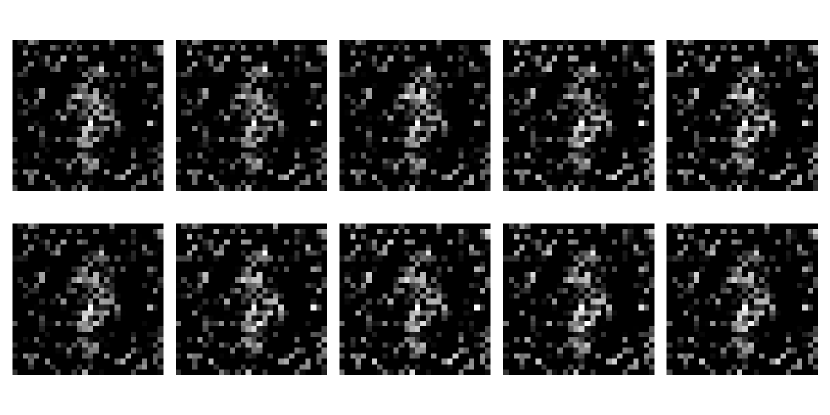
(e) 15386 parameters removed (98.1%). Equivalent to cutoff $\Lambda=1.75$.

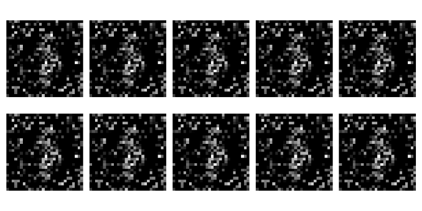
(f) All (15680) parameters removed (100%). Maximal information loss. Equivalent to cutoff $\Lambda=2.375$.

Figure 4: Randomly pruned network with equivalent numbers of removed parameters to Figure 3.

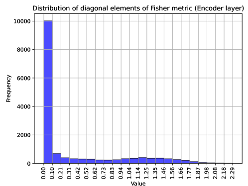
Figure 5: Histogram showing the distribution of diagonal Fisher matrix elements.

5 Discussion

In this note we have outlined a new perspective on renormalization that is fully information theoretic in nature. As a consequence, this approach to renormalization is amenable to arbitrary probability models, not just those which possess a physical interpretation. The major insight we have presented is that the Fisher metric should be interpreted as defining a correlation length in the space of models which defines an emergent scale through the distinguishability of probability distributions. From this perspective, a UV cutoff in a Bayesian renormalization scheme can be understood as fixing the maximum number of possible measurements that could be made about a system, thereby bounding the precision with which one can access information about the data generating model in an inference experiment. This perspective on renormalization is consistent with the more familiar physical picture where the amount of data that can be collected about a theory is bounded by the energy scales which can be probed experimentally. Hence, again, the UV cut-off dictates the set of possible independent measurements. More rigorously, this observation can be quantified through the observation that the KL-divergence is a ERG monotone [41], or the fact that even in RG schemes with a physical scale the ERG kernel can be identified with the Fisher metric on the space of theories [77].

The information theoretic approach to renormalization allows for a very satisfying connection to be made between renormalization and techniques from data science such as model selection, data compression, and data generation. Among the most important insights that arise from using the Fisher metric to define the emergent RG scale is that “high energy modes” are naturally identified with “sloppy” parameters which are systematically discarded to formulate “low energy” effective theories that depend only on “strict” parameters. In this respect, we regard Bayesian Renormalization as an information geometrically inspired coarse-graining scheme. A related perspective on the relationship between renormalization and data compression has been studied through the so called information bottleneck, for a representative sample of papers on the topic see [19, 20, 21, 36]. The basic idea here is that the information bottleneck identifies a set of low dimensional effective degrees of freedom which efficiently encode the data contained in an otherwise high dimensional space of data realizations. Moving from the original degrees of freedom to the effective degrees of freedom involves a stochastic mapping (conditional probability distribution) which may be interpreted as a form of coarse graining based renormalization. In addition to the connection with data compression, the framing of Bayesian renormalization as a stochastic diffusion process allows one to interpret it as a refinement on the influential diffusion learning paradigm introduced in [42]. The duality between renormalization and statistical learning provides new context for the usefulness of score based generative algorithms for inverting diffusion processes.

At the moment the connections we have addressed are largely conceptual, but in future work we hope to demonstrate how the understanding of Bayesian renormalization can contribute to new automated techniques for data compression and data generation. As a first pass at this problem, we have explored a simple implementation of Bayesian renormalization to a Neural Network in Section 4 to illustrate some of its most salient and useful features. The most crucial insight from this example is that Fisher inspired renormalization can systematically discard degrees of freedom in a hierarchy of importance relative to the model in question. The specific approach we used is a one-to-one adaptation of Wilson’s momentum shell renormalization scheme in which momentum shells are replaced by regions of fixed radius in the space of models according to the measure of distance defined by the Fisher metric. No assumptions about the structure or symmetries of the data or model were required in order to perform the aforementioned renormalization. Rather, the structure of the system is learned and subsequently encoded in the hierarchy of scales communicated by the Fisher metric.

Although we have concentrated primarily on the value of the information theoretic character of Bayesian renormalization in data science contexts, let us close by noting that this approach to renormalization may also provide new insights in physics contexts as well. For starters, the information theoretic approach of Bayesian renormalization makes it an ideal tool for identifying and quantifying the precise information that is lost under an RG flow. In this way, one should be able to use Bayesian renormalization in order to interpret and construct RG monotonicity theorems [78, 79, 80, 81, 82, 83]. On a different note, a modern perspective on renormalization would not be complete without including Entanglement/Holographic Renormalization: [84, 85, 86, 87, 88, 89, 47, 90]. It is a challenge for future work to bring together Bayesian renormalization described in this paper with the holographic description of renormalization that has been developed in the above works. Of relevance to this is the relationship between canonical energy and Fisher metric in holographic context: [91, 92, 93, 94, 95]. Finally, the different ways that energy scales with entropy in a physical system tell us about the effectiveness of the usual momentum-based renormalization. An interesting question that one might ask is whether there is a different way of performing renormalization that more appropriately coarse grains information. In particular, large momentum shells may not be the right “sloppy parameters” for a gravitation theory. Recall that the scaling of entropy with energy is different in gravity from that of local quantum field theories. This is a key ingredient that allows the holographic property of gravity. The perspective presented here is that the energy cut-off is really an information cut-off. As such this information theoretic perspective suggests that one might consider a different cut-off scheme for gravity than one uses for QFT. This is the power of the Bayesian Renormalization principle: it automatically encodes the appropriate designation of relevant and irrelevant degrees of freedom through the Fisher metric and thus ensures that the degrees of freedom that are “integrated out of the model” correspond precisely with the sloppy parameters, whatever they may be.

References

- [1] E. T. Jaynes, Information theory and statistical mechanics, Physical review 106 (1957), no. 4 620.
- [2] E. T. Jaynes, Probability theory: The logic of science. Cambridge university press, 2003.
- [3] A. Gelman and C. R. Shalizi, Philosophy and the practice of bayesian statistics, British Journal of Mathematical and Statistical Psychology 66 (2013), no. 1 8–38.
- [4] D. S. Berman, J. J. Heckman, and M. Klinger, On the dynamics of inference and learning, arXiv:2204.12939.
- [5] L. P. Kadanoff, Scaling laws for Ising models near t c, Physics Physique Fizika 2 (1966), no. 6 263.
- [6] K. G. Wilson, Renormalization group and critical phenomena. i. renormalization group and the kadanoff scaling picture, Physical review B 4 (1971), no. 9 3174.
- [7] K. G. Wilson and J. Kogut, The renormalization group and the expansion, Physics reports 12 (1974), no. 2 75–199.
- [8] F. Wegner, Some invariance properties of the renormalization group, Journal of Physics C: Solid State Physics 7 (1974), no. 12 2098.
- [9] F. J. Wegner and A. Houghton, Renormalization group equation for critical phenomena, Physical Review A 8 (1973), no. 1 401.
- [10] J. Polchinski, Renormalization and effective lagrangians, Nuclear Physics B 231 (1984), no. 2 269–295.
- [11] T. R. Morris, Derivative expansion of the exact renormalization group, Physics Letters B 329 (1994), no. 2-3 241–248, [hep-ph/9403340v2].
- [12] T. R. Morris, The exact renormalization group and approximate solutions, International Journal of Modern Physics A 9 (1994), no. 14 2411–2449.
- [13] T. R. Morris, Elements of the continuous renormalization group, Progress of Theoretical Physics Supplement 131 (1998) 395–414, [hep-th/9802039v1].
- [14] J. I. Latorre and T. R. Morris, Exact scheme independence, Journal of High Energy Physics 2000 (2000), no. 11 004, [hep-th/0008123v2].
- [15] C. Bagnuls and C. Bervillier, Exact renormalization group equations: an introductory review, Physics Reports 348 (2001), no. 1-2 91–157, [hep-th/0002034].
- [16] T. R. Morris and O. J. Rosten, Manifestly gauge invariant QCD, J. Phys. A 39 (2006) 11657–11681, [hep-th/0606189].
- [17] O. J. Rosten, Fundamentals of the exact renormalization group, Physics Reports 511 (2012), no. 4 177–272, [arXiv:1003.1366].
- [18] D. S. Berman and M. S. Klinger, The Inverse of Exact Renormalization Group Flows as Statistical Inference, arXiv:2212.11379.
- [19] L. Meshulam, J. L. Gauthier, C. D. Brody, D. W. Tank, and W. Bialek, Coarse graining, fixed points, and scaling in a large population of neurons., Physical review letters 123 17 (2018) 178103, [arXiv:1809.08461].
- [20] L. Meshulam, J. L. Gauthier, C. D. Brody, D. W. Tank, and W. Bialek, Coarse–graining and hints of scaling in a population of 1000+ neurons, arXiv: Biological Physics (2018) [arXiv:1812.11904].
- [21] A. G. Kline and S. E. Palmer, Gaussian information bottleneck and the non-perturbative renormalization group, New J. Phys. 24 (2022), no. 3 033007, [arXiv:2107.13700].
- [22] P. Mehta and D. J. Schwab, An exact mapping between the variational renormalization group and deep learning, arXiv:1410.3831.
- [23] H. W. Lin, M. Tegmark, and D. Rolnick, Why Does Deep and Cheap Learning Work So Well?, J. Statist. Phys. 168 (2017), no. 6 1223–1247, [arXiv:1608.08225].
- [24] J. Halverson, A. Maiti, and K. Stoner, Neural Networks and Quantum Field Theory, Mach. Learn. Sci. Tech. 2 (2021), no. 3 035002, [arXiv:2008.08601].
- [25] D. Luo and J. Halverson, Infinite Neural Network Quantum States, arXiv:2112.00723.
- [26] J. Halverson, Building Quantum Field Theories Out of Neurons, arXiv:2112.04527.
- [27] A. R. Brown, M. H. Freedman, H. W. Lin, and L. Susskind, Effective Geometry, Complexity, and Universality, arXiv:2111.12700.
- [28] Y.-H. He, E. Heyes, and E. Hirst, Machine Learning in Physics and Geometry, arXiv:2303.12626.
- [29] J. Erdmenger, K. T. Grosvenor, and R. Jefferson, Towards quantifying information flows: relative entropy in deep neural networks and the renormalization group, 2021.
- [30] S.-i. Amari and H. Nagaoka, Methods of information geometry, vol. 191. American Mathematical Soc., 2000.
- [31] S.-i. Amari, Information geometry and its applications, vol. 194. Springer, 2016.
- [32] F. Nielsen, An elementary introduction to information geometry, Entropy 22 (2020), no. 10 1100, [arXiv:1808.08271].
- [33] C. Strandkvist, P. Chvykov, and M. Tikhonov, Beyond RG: from parameter flow to metric flow, arXiv:2011.12420.
- [34] K. N. Quinn, M. C. Abbott, M. K. Transtrum, B. B. Machta, and J. P. Sethna, Information geometry for multiparameter models: New perspectives on the origin of simplicity, arXiv:2111.07176.
- [35] V. Balasubramanian, J. J. Heckman, and A. Maloney, Relative Entropy and Proximity of Quantum Field Theories, JHEP 05 (2015) 104, [arXiv:1410.6809].
- [36] A. Gordon, A. Banerjee, M. Koch-Janusz, and Z. Ringel, Relevance in the renormalization group and in information theory, Phys. Rev. Lett. 126 (Jun, 2021) 240601, [arXiv:2012.01447].
- [37] N. Tishby, F. C. Pereira, and W. Bialek, The information bottleneck method, physics/0004057.
- [38] C. Bény and T. J. Osborne, Information-geometric approach to the renormalization group, Phys. Rev. A 92 (2015), no. 2 022330, [arXiv:1206.7004].
- [39] C. Bény and T. J. Osborne, The renormalization group via statistical inference, New J. Phys. 17 (2015), no. 8 083005, [arXiv:1402.4949].
- [40] A. Raju, B. B. Machta, and J. P. Sethna, Information loss under coarse graining: A geometric approach, Physical Review E 98 (nov, 2018) [arXiv:1710.05787].
- [41] J. Cotler and S. Rezchikov, Renormalization group flow as optimal transport, arXiv:2202.11737.
- [42] J. Sohl-Dickstein, E. A. Weiss, N. Maheswaranathan, and S. Ganguli, Deep unsupervised learning using nonequilibrium thermodynamics, arXiv:1503.03585.
- [43] J. Cardy, Introduction to quantum field theory, Michaelmas Term (2010).
- [44] M. E. Peskin, D. V. Schroeder, and E. Martinec, An Introduction to Quantum Field Theory, Physics Today 49 (08, 1996).
- [45] M. Matsumoto, G. Tanaka, and A. Tsuchiya, The renormalization group and the diffusion equation, Progress of Theoretical and Experimental Physics 2021 (dec, 2020).
- [46] T. Faulkner, The holographic map as a conditional expectation, arXiv:2008.04810.
- [47] K. Furuya, N. Lashkari, and S. Ouseph, Real-space RG, error correction and petz map, Journal of High Energy Physics 2022 (Jan, 2022) [arXiv:2012.14001].
- [48] E. Gesteau, Large von Neumann algebras and the renormalization of Newton’s constant, arXiv:2302.01938.
- [49] M. Takesaki, Conditional expectations in von Neumann algebras, Journal of Functional Analysis 9 (1972), no. 3 306–321.
- [50] E. A. Carlen and J. Maas, An analog of the 2-wasserstein metric in non-commutative probability under which the fermionic fokker–planck equation is gradient flow for the entropy, Communications in mathematical physics 331 (2014), no. 3 887–926, [arXiv:1203.5377].
- [51] E. A. Carlen and J. Maas, Gradient flow and entropy inequalities for quantum markov semigroups with detailed balance, Journal of Functional Analysis 273 (2017), no. 5 1810–1869, [arXiv:1609.01254].
- [52] E. A. Carlen and J. Maas, Non-commutative calculus, optimal transport and functional inequalities in dissipative quantum systems, Journal of Statistical Physics 178 (2020), no. 2 319–378, [arXiv:1811.04572].
- [53] Y. Song, J. Sohl-Dickstein, D. P. Kingma, A. Kumar, S. Ermon, and B. Poole, Score-based generative modeling through stochastic differential equations, arXiv preprint arXiv:2011.13456 (2020).
- [54] B. D. Anderson, Reverse-time diffusion equation models, Stochastic Processes and their Applications 12 (1982), no. 3 313–326.
- [55] Ö. Legeza and J. Sólyom, Quantum data compression, quantum information generation, and the density-matrix renormalization-group method, Physical Review B 70 (2004), no. 20 205118, [cond-mat/0401136].
- [56] D. P. Kingma and M. Welling, Auto-Encoding Variational Bayes, arXiv:1312.6114.
- [57] B. B. Machta, R. Chachra, M. K. Transtrum, and J. P. Sethna, Parameter space compression underlies emergent theories and predictive models, Science 342 (nov, 2013) 604–607, [arXiv:1303.6738].
- [58] D. Kingma, T. Salimans, B. Poole, and J. Ho, Variational diffusion models, Advances in neural information processing systems 34 (2021) 21696–21707, [arXiv:2107.00630].
- [59] J. Gui, Z. Sun, Y. Wen, D. Tao, and J. Ye, A review on generative adversarial networks: Algorithms, theory, and applications, IEEE transactions on knowledge and data engineering (2021) [arXiv:2001.06937].
- [60] A. Ramesh, M. Pavlov, G. Goh, S. Gray, C. Voss, A. Radford, M. Chen, and I. Sutskever, Zero-shot text-to-image generation, in International Conference on Machine Learning, pp. 8821–8831, PMLR, 2021.
- [61] A. Ramesh, P. Dhariwal, A. Nichol, C. Chu, and M. Chen, Hierarchical text-conditional image generation with CLIP latents, arXiv:2204.06125.
- [62] Y. Teng, S. Sachdev, and M. S. Scheurer, Classifying topological neural network quantum states via diffusion maps, arXiv:2301.02683.
- [63] A. Bansal, E. Borgnia, H.-M. Chu, J. S. Li, H. Kazemi, F. Huang, M. Goldblum, J. Geiping, and T. Goldstein, Cold diffusion: Inverting arbitrary image transforms without noise, arXiv:2208.09392.
- [64] K. Fischer, A. René, C. Keup, M. Layer, D. Dahmen, and M. Helias, Decomposing neural networks as mappings of correlation functions, Physical Review Research 4 (2022), no. 4 043143, [arXiv:2202.04925].
- [65] P. Fleig and I. Nemenman, Statistical properties of large data sets with linear latent features, Physical Review E 106 (jul, 2022) [arXiv:2111.04641].
- [66] J. F. Rodriguez-Nieva and M. S. Scheurer, Identifying topological order through unsupervised machine learning, Nature Physics 15 (may, 2019) 790–795, [arXiv:1805.05961].
- [67] R. M. Neal, Annealed importance sampling, Statistics and computing 11 (2001), no. 2 125–139, [physics/9803008v2].
- [68] Y. Bahri, E. Dyer, J. Kaplan, J. Lee, and U. Sharma, Explaining neural scaling laws, arXiv:2102.06701.
- [69] B. C. Daniels, Y.-J. Chen, J. P. Sethna, R. N. Gutenkunst, and C. R. Myers, Sloppiness, robustness, and evolvability in systems biology, Current opinion in biotechnology 19 (2008), no. 4 389–395, [arXiv:0805.2628].
- [70] M. K. Transtrum, B. B. Machta, K. S. Brown, B. C. Daniels, C. R. Myers, and J. P. Sethna, Perspective: Sloppiness and emergent theories in physics, biology, and beyond, The Journal of chemical physics 143 (2015), no. 1 07B201_1.
- [71] M. C. Abbott and B. B. Machta, Far from asymptopia, arXiv:2205.03343.
- [72] M. Dashti and A. M. Stuart, The Bayesian approach to inverse problems, arXiv:1302.6989.
- [73] L. Wasserman, All of statistics: a concise course in statistical inference, vol. 26. Springer, 2004.
- [74] L. V. Jospin, H. Laga, F. Boussaid, W. Buntine, and M. Bennamoun, Hands-on bayesian neural networks—a tutorial for deep learning users, IEEE Computational Intelligence Magazine 17 (may, 2022) 29–48.
- [75] T. George, NNGeometry: Easy and Fast Fisher Information Matrices and Neural Tangent Kernels in PyTorch, Feb., 2021.
- [76] D. P. Kingma and J. Ba, Adam: A method for stochastic optimization, 2017.
- [77] S. Floerchinger, Exact flow equation for the divergence functional, arXiv:2303.04082.
- [78] A. B. Zamolodchikov, Irreversibility of the flux of the renormalization group in a 2d field theory, JETP lett 43 (1986), no. 12 730–732.
- [79] E. Alvarez and C. Gomez, Geometric holography, the renormalization group and the c-theorem, Nuclear Physics B 541 (1999), no. 1-2 441–460, [hep-th/9807226v1].
- [80] R. C. Myers and A. Sinha, Seeing a c-theorem with holography, Physical Review D 82 (2010), no. 4 046006, [arXiv:1006.1263].
- [81] H. Casini and M. Huerta, A c-theorem for entanglement entropy, Journal of Physics A: Mathematical and Theoretical 40 (2007), no. 25 7031.
- [82] H. Casini, M. Huerta, R. C. Myers, and A. Yale, Mutual information and the f-theorem, Journal of High Energy Physics 2015 (2015), no. 10 1–70, [arXiv:1506.06195].
- [83] H. Casini, E. Testé, and G. Torroba, Markov property of the conformal field theory vacuum and the a theorem, Physical review letters 118 (2017), no. 26 261602.
- [84] B. Swingle, Entanglement renormalization and holography, Physical Review D 86 (2012), no. 6 065007, [arXiv:0905.1317].
- [85] M. Nozaki, S. Ryu, and T. Takayanagi, Holographic geometry of entanglement renormalization in quantum field theories, Journal of High Energy Physics 2012 (2012), no. 10 1–40, [arXiv:1208.3469].
- [86] A. Mollabashi, M. Naozaki, S. Ryu, and T. Takayanagi, Holographic geometry of cMERA for quantum quenches and finite temperature, Journal of High Energy Physics 2014 (2014), no. 3 1–30, [arXiv:1311.6095].
- [87] R. G. Leigh, O. Parrikar, and A. B. Weiss, Holographic geometry of the renormalization group and higher spin symmetries, Physical Review D 89 (2014), no. 10 106012, [arXiv:1402.1430].
- [88] R. G. Leigh, O. Parrikar, and A. B. Weiss, Exact renormalization group and higher-spin holography, Phys. Rev. D 91 (2015), no. 2 026002, [arXiv:1407.4574].
- [89] G. Evenbly and G. Vidal, Tensor network renormalization, Physical review letters 115 (2015), no. 18 180405, [arXiv:1412.0732].
- [90] S. Goldman, N. Lashkari, R. G. Leigh, and M. Moosa, Exact renormalization of wave functionals yields continuous MERA, arXiv:2301.09669.
- [91] N. Lashkari, Modular Hamiltonian for Excited States in Conformal Field Theory, Phys. Rev. Lett. 117 (2016), no. 4 041601, [arXiv:1508.03506].
- [92] N. Lashkari and M. Van Raamsdonk, Canonical energy is quantum Fisher information, Journal of High Energy Physics 2016 (2016), no. 4 1–26, [arXiv:1508.00897].
- [93] S. Banerjee, J. Erdmenger, and D. Sarkar, Connecting Fisher information to bulk entanglement in holography, Journal of High Energy Physics 2018 (aug, 2018) [arXiv:1701.02319].
- [94] T. Faulkner, F. M. Haehl, E. Hijano, O. Parrikar, C. Rabideau, and M. V. Raamsdonk, Nonlinear gravity from entanglement in conformal field theories, Journal of High Energy Physics 2017 (aug, 2017) [arXiv:1705.03026].
- [95] J. Erdmenger, K. Grosvenor, and R. Jefferson, Information geometry in quantum field theory: lessons from simple examples, SciPost Physics 8 (May, 2020).
- [96] L. Freidel, J. Kowalski-Glikman, R. G. Leigh, and D. Minic, The Vacuum Energy Density and Gravitational Entropy, arXiv:2212.00901.
- [97] L. Freidel, J. Kowalski-Glikman, R. G. Leigh, and D. Minic, On the Inevitable Lightness of Vacuum, arXiv:2303.17495.