Topological superconductivity in two-dimensional altermagnetic metals

Abstract

Bringing magnetic metals into superconducting states represents an important approach for realizing unconventional superconductors and potentially even topological superconductors. Altermagnetism, classified as a third basic collinear magnetic phase, gives rise to intriguing momentum-dependent spin-splitting of the band structure, and results in an even number of spin-polarized Fermi surfaces due to the symmetry-enforced zero net magnetization. In this work, we investigate the effect of this new magnetic order on the superconductivity of a two-dimensional metal with $d$-wave altermagnetism and Rashba spin-orbital coupling. Specifically we consider an extended attractive Hubbard interaction, and determine the types of superconducting pairing that can occur in this system and ascertain whether they possess topological properties. Through self-consistent mean-field calculations, we find that the system in general favors a mixture of spin-singlet $s$-wave and spin-triplet $p$-wave pairings, and that the altermagnetism is beneficial to the latter. Using symmetry arguments supported by detailed calculations, we show that a number of topological superconductors, including both first-order and second-order ones, can emerge when the $p$-wave pairing dominates. In particular, we find that the second-order topological superconductor is enforced by a $\mathcal{C}_{4z}\mathcal{T}$ symmetry, which renders the spin polarization of Majorana corner modes into a unique entangled structure. Our study demonstrates that altermagnetic metals are fascinating platforms for the exploration of intrinsic unconventional superconductivity and topological superconductivity.

I Introduction

Magnetism and superconductivity are two fundamental phenomena in nature, whose interplay in materials is one of the central topics in condensed matter physics Scalapino et al. (1986); T. Moriya and Ueda (1990); Monthoux et al. (1991); Mathur et al. (1998); Saxena et al. (2000); Aoki et al. (2001); Mito et al. (2003); Akazawa et al. (2004); Huy et al. (2007); Li et al. (2011); Bert et al. (2011); Dikin et al. (2011). Magnetism can influence superconductivity in many ways, and its effect on the pairing symmetry is of particular interest Bergeret et al. (2005); Scalapino (2012). Generally speaking, magnetism is detrimental to spin-singlet superconductivity but is conducive to the emergence of unconventional superconductivity. Take ferromagnetism for example. Its adverse effect on spin-singlet pairings can be attributed to the breaking of time-reversal symmetry (TRS) which lifts the spin degeneracy of the electronic bands; this results in spin-split Fermi surfaces on which electrons can no longer find time-reversal partners to form spin-singlet Cooper pairs. Fortunately, a realistic system admits of many competing pairing channels Sigrist and Ueda (1991). While the spin-singlet pairing normally wins out in time-reversal invariant systems, its suppression by magnetism means that other unconventional pairings could stand to benefit.

Recently, it has been observed in a series of materials with compensated magnetization that a third basic collinear magnetic order Šmejkal et al. (2020); Hayami et al. (2019, 2020); Yuan et al. (2020, 2021); Mazin et al. (2021); Liu et al. (2022); Feng et al. (2022a); Gonzalez Betancourt et al. (2023); Mazin (2023); Turek (2022); Guo et al. (2023); Hariki et al. (2023); Zhou et al. (2023), referred to as altermagnetism (AM) Šmejkal et al. (2022a, b, c), exists beyond the conventional dichotomy between ferromagnetism and antiferromagnetism. The nomenclature is intended to convey the most important characteristic of this new magnetic order: that the spin polarization alternates in both coordinate and momentum spaces. The effect of AM on the electronic band structure is rather different from those of the ferromagnetism or antiferromagnetism. Unlike usual antiferromagnetism due to symmetry reason Yuan et al. (2020, 2021), AM results in momentum-dependent spin splitting to the band structure, resembling a spin-orbital coupling effect but without spin-momentum locking Šmejkal et al. (2022c). Although these spin-split bands also lead to spin-polarized Fermi surfaces like in ferromagnetic metals, the Fermi surfaces are generally anisotropic as a result of the momentum-dependent spin polarization. In addition, the number of spin-polarized Fermi surfaces in AM metals is constrained to be even due to the symmetry-enforced zero net magnetization. Because of these unique properties, AM metals are emerging as another intriguing class of systems to study the interaction between magnetism and superconductivity Mazin (2022). Several novel phenomena, such as orientation-dependent Andreev reflection Sun et al. (2023); Papaj (2023), Josephson effect Ouassou et al. (2023) and finite-momentum Cooper pairing Zhang et al. (2023), have already been predicted in heterostructures composed of AM materials and superconductors. Notably, some parent compounds of high-temperature superconductors are revealed to be altermagnets Šmejkal et al. (2022b, c), raising the prospect that the coexistence of AM and superconductivity may be observed in a single material. However, the study of AM in general is still at an early stage, and fundamental questions such as what types of superconductivity may emerge in AM metals and whether they are topological remain to be answered.

In this work, we address these questions in the context of two-dimensional (2D) metals with $d$-wave AM Šmejkal et al. (2022c) and Rashba spin-orbital coupling (RSOC). We incorporate the RSOC because it arises naturally when the AM metal is grown on a substrate Bychkov and Rashba (1984). Focusing on representative short-range attractive interactions allowing for both $s$ and $p$-wave pairing channels, we first determine the pairing phase diagram spanned by the RSOC strength and the relative $s$-to-$p$-wave pairing interaction strength. Our calculations show that the AM metal with RSOC favors a mixture of spin-singlet $s$-wave and spin-triplet $p$-wave pairings, in contrast to the case of pure $s$ or $p$-wave pairings without RSOC; such mixed parity pairings are a result of the simultaneous breaking of the TRS by AM and the inversion symmetry by RSOC. For finite RSOC, two mixed parity pairing phases are found, namely the $s$ $+$ helical $p$-wave phase and the $s$ $+$ chiral $p$-wave phase. Notably, the former can prevail over the latter for weak RSOC strengths even though the TRS is broken. We further investigate the topological properties of these pairings and identify a crucial set of symmetries that can be used to delineate various topological phases. Using symmetry arguments corroborated by detailed calculations, we show that the superconducting phase is topologically trivial when the $s$-wave pairing dominates, regardless of the nature of the $p$-wave component; on the other hand, a multitude of topologically non-trivial phases can be realized when the $p$-wave pairing dominates. Specifically, it realizes a chiral TSC Read and Green (2000); Sato et al. (2009); Qi et al. (2010); Sau et al. (2010); Alicea (2010) characterized by an even Chern number for dominant chiral-$p$ wave pairings, and a helical TSC or a second-order TSC for dominant helical-$p$ wave pairings. In the latter scenario, the superconductor is a helical TSC Qi et al. (2009); Deng et al. (2012); Nakosai et al. (2012); Zhang et al. (2013a); Wang et al. (2014); Midtgaard et al. (2017); Huang and Chiu (2018); Zhang and Das Sarma (2021); Feng et al. (2022b) if, as in the case of no RSOC, a mirror symmetry or subsystem chiral symmetry exists to protect the helical Majorana modes; otherwise, it becomes a second-order TSC with Majorana corner modes Langbehn et al. (2017); Geier et al. (2018); Khalaf (2018); Zhu (2018); Yan et al. (2018); Wang et al. (2018a, b); Liu et al. (2018); Wu et al. (2019); Yan (2019); Volpez et al. (2019); Zhang et al. (2019); Pan et al. (2019); Zhu (2019); Hsu et al. (2020); Wu et al. (2020a); Kheirkhah et al. (2020); Wu et al. (2020b); Qin et al. (2022); Zhu et al. (2022); Li et al. (2021); Scammell et al. (2022) when these symmetries are broken by finite RSOC. These results spotlight 2D superconducting AM metals as a remarkable platform in which both 1D and 0D Majorana modes can be achieved.

II Model and results

II.1 2D metals with $d$-wave AM and RSOC

We consider a 2D metal with $d$-wave AM described by the Hamiltonian $\hat{H}_{0}=\sum_{\boldsymbol{k}\sigma}h_{\sigma\sigma^{\prime}}(\boldsymbol{k})c_{\boldsymbol{k}\sigma}^{\dagger}c_{\boldsymbol{k}\sigma^{\prime}}$. Expressed in terms of the Pauli matrices $\sigma_{x,y,z}$ and the identity matrix $\sigma_{0}$, $h_{\sigma\sigma^{\prime}}(\boldsymbol{k})$ is given by (lattice constant is set to unity throughout) Šmejkal et al. (2022c)

$$h(\boldsymbol{k}) = -2t(\cos k_{x}+\cos k_{y})\sigma_{0}+2t_{\rm AM}(\cos k_{x}-\cos k_{y})\sigma_{z}$$ (1)

$$+2\lambda(\sin k_{y}\sigma_{x}-\sin k_{x}\sigma_{y}),$$

where the $t_{\rm AM}$ term and the $\lambda$ term describe the exchange field associated with AM and the RSOC respectively. We note that the momentum dependence of the AM exchange field resembles that of the $d$-wave pairing in high-$T_{c}$ superconductors Tsuei and Kirtley (2000).

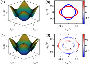
Figure 1: (Color online) Band structures (left) and Fermi surfaces (right) of the AM metal with and without RSOC. (a)-(b), $\lambda=0$; (c)-(d), $\lambda=0.2$. The color of the Fermi surfaces indicates the magnitude of $\langle\sigma_{z}\rangle$, and the length and direction of the arrows indicate the magnitude and direction of the in-plane spin polarization. The spin textures clearly display the $\mathcal{C}_{4z}\mathcal{T}$ symmetry. Common parameters are $t=0.5$, $t_{\rm AM}=0.1$, and $\mu=-1$.

The AM exchange field brings significant changes to the original band structure given by the first term of Eq. (1). First, it breaks the TRS $\mathcal{T}=-i\sigma_{y}\mathcal{K}$ ($\mathcal{K}$ is the complex conjugation operator) and gives rise to spin-split bands. Second, its $d$-wave nature breaks the 4-fold rotational symmetry $\mathcal{C}_{4z}=e^{i\frac{\pi}{4}\sigma_{z}}$ and results in the deformation of the Fermi surfaces. Both features can be clearly seen in Figs. 1(a) and  1(b). Now, the additional RSOC also has important effects on the band structure. Because it breaks both the inversion symmetry $\mathcal{P}=\sigma_{0}$ and the mirror symmetry $\mathcal{M}_{z}=i\sigma_{z}$ of the AM metal, the remaining degeneracies along the $|k_{x}|=|k_{y}|$ axes are removed (see Fig. 1(c)). Furthermore, it introduces spin-momentum locking on the spin-polarized Fermi surfaces, as shown in Fig.1(d). All these properties play a role in determining the pairing symmetry and topological properties of the superconducting phases.

Another interesting fact about the Hamiltonian in Eq. (1) is that it preserves the overall $\mathcal{C}_{4z}\mathcal{T}$ symmetry; this can be seen from the fact that all three terms in Eq. (1) respect this symmetry. Two important properties of the AM metallic state immediately follow from this observation. First, the net magnetization of the metallic state must be zero even though the two bands become spin-split. Second, such a state can be viewed as a critical metallic phase. To see this, we first note that the Kramers theorem dictates the existence of band degeneracies at the two $\mathcal{C}_{4z}\mathcal{T}$-invariant momenta, i.e., $\boldsymbol{\Gamma}=(0,0)$ and $\boldsymbol{M}=(\pi,\pi)$, as shown in Fig.1(c). Thus, an arbitrarily small out-of-plane magnetic field, which breaks the $\mathcal{C}_{4z}\mathcal{T}$ symmetry, will open a gap at $\boldsymbol{\Gamma}$ and $\boldsymbol{M}$ and drive the system to be a Chern metal where the two bands will carry opposite Chern numbers $C=\pm 1$ Qi et al. (2006) (see Appendix A). In addition, a reversal of the magnetic field’s direction will reverse the Chern number of the two bands. Such a critical behavior is a manifestation of the fact that the band structure of AM metals differs drastically from those of ferromagnetic and antiferromagnetic metals.

II.2 Pairing phase diagram

The pairing mechanism in a magnetic metal is known to be non-unique Monthoux et al. (2007), and the effects of magnetism on superconductivity are also known to be diverse. Importantly, magnetism and superconductivity are not always exclusive. Indeed, the coexistence of magnetic and superconducting orders has been observed in many materials, ranging from heavy-fermion systems Saxena et al. (2000); Aoki et al. (2001); Mito et al. (2003); Akazawa et al. (2004); Huy et al. (2007) to oxide interfaces Li et al. (2011); Bert et al. (2011); Dikin et al. (2011). In this work, we do not examine the microscopic origin of the pairing interaction and instead assume the following extended attractive Hubbard interaction

$$\hat{H}_{int}=-V_{s}\sum_{i}n_{i\uparrow}n_{i\downarrow}-V_{p}\sum_{\langle ij\rangle,\sigma}n_{i\sigma}n_{j\sigma},$$ (2)

where $n_{i\sigma}$ is the density operator for electrons of spin $\sigma$ on site $i$, and $V_{s}$ and $V_{p}$ are respectively the strengths of the on-site and nearest-neighbor attraction. Equation (2) is a minimal form of interaction that is capable of describing the competition between spin-singlet and spin triplet pairings.

Following the standard BCS theory, we define the gap function as

$$\Xi_{\sigma\sigma^{\prime}}(\boldsymbol{k})=-\frac{1}{N_{L}}\sum_{\boldsymbol{k}^{\prime}}V_{{\sigma\sigma^{\prime}}}(\boldsymbol{k}-\boldsymbol{k}^{\prime})\langle c_{\boldsymbol{k}^{\prime}\sigma}c_{-\boldsymbol{k}^{\prime}\sigma^{\prime}}\rangle,$$ (3)

where $N_{L}$ is the number of lattice sites and $V_{\sigma\sigma^{\prime}}(\boldsymbol{q})=-(1-\delta_{\sigma,\sigma^{\prime}})V_{s}-\delta_{\sigma,\sigma^{\prime}}2V_{p}(\cos q_{x}+\cos q_{y})$ is the interaction in Fourier space. The pair correlation can be calculated in terms of the Bogoliubov amplitudes as

$$\langle c_{\boldsymbol{k}\sigma}c_{-\boldsymbol{k}\sigma^{\prime}}\rangle=u_{\sigma,1}(\boldsymbol{k})v_{\sigma^{\prime},1}^{*}(\boldsymbol{k})+u_{\sigma,2}(\boldsymbol{k})v_{\sigma^{\prime},2}^{*}(\boldsymbol{k}).$$ (4)

These amplitudes are determined by the Bogoliubov-de Gennes (BdG) equation $\mathcal{H}_{\rm BdG}(\boldsymbol{k})\chi_{\boldsymbol{k},l}=E_{\boldsymbol{k},l}\chi_{\boldsymbol{k},l}$, where $E_{\boldsymbol{k},l}$ with $l=\{1,2\}$ refer to the two positive eigenenergies, $\chi_{\boldsymbol{k},l}\equiv[u_{\uparrow,l}(\boldsymbol{k}),u_{\downarrow,l}(\boldsymbol{k}),v_{\uparrow,l}(\boldsymbol{k}),v_{\downarrow,l}(\boldsymbol{k})]^{T}$ are the corresponding eigenstates, and

$$\mathcal{H}_{\rm BdG}(\boldsymbol{k})=\begin{bmatrix}\xi_{\boldsymbol{k}\uparrow}&\Lambda(\boldsymbol{k})&\Xi_{\uparrow\uparrow}(\boldsymbol{k})&\Xi_{\uparrow\downarrow}(\boldsymbol{k})\\ \Lambda^{*}(\boldsymbol{k})&\xi_{\boldsymbol{k}\downarrow}&\Xi_{\downarrow\uparrow}(\boldsymbol{k})&\Xi_{\downarrow\downarrow}(\boldsymbol{k})\\ \Xi^{*}_{\uparrow\uparrow}(\boldsymbol{k})&\Xi^{*}_{\downarrow\uparrow}(\boldsymbol{k})&-\xi_{\boldsymbol{k}\uparrow}&-\Lambda^{*}(-\boldsymbol{k})\\ \Xi^{*}_{\uparrow\downarrow}(\boldsymbol{k})&\Xi^{*}_{\downarrow\downarrow}(\boldsymbol{k})&-\Lambda(-\boldsymbol{k})&-\xi_{\boldsymbol{k}\downarrow}\end{bmatrix}.$$ (5)

Here $\Lambda(\boldsymbol{k})=2\lambda(\sin k_{y}+i\sin k_{x})$ and $\xi_{\boldsymbol{k}s}=-2(t-st_{\rm AM})\cos k_{x}-2(t+st_{\rm AM})\cos k_{y}-\mu$ where $s=1$ ($-1$) for spin up (down).

To determine possible pairing channels, one may expand both $V_{\sigma\sigma^{\prime}}({\boldsymbol{k}-\boldsymbol{k}^{\prime}})$ and $\Xi_{\sigma\sigma^{\prime}}(\boldsymbol{k})$ in terms of the so-called square lattice harmonics $g_{\eta}(\boldsymbol{k})$ (see Appendix B), i.e.,

$$V_{\sigma\sigma^{\prime}}({\boldsymbol{k}-\boldsymbol{k}^{\prime}}) =\sum_{\eta}\gamma^{\eta}_{\sigma\sigma^{\prime}}g_{\eta}(\boldsymbol{k})g_{\eta}^{*}(\boldsymbol{k}^{\prime});$$ (6)

$$\Xi_{\sigma\sigma^{\prime}}(\boldsymbol{k}) =\sum_{\eta}\Delta_{\sigma\sigma^{\prime}}^{\eta}g_{\eta}(\boldsymbol{k}),$$ (7)

where $\gamma^{\eta}_{\sigma\sigma^{\prime}}$ is the strength of the pairing interaction in the $\eta$-channel. For the attractive interaction given in Eq.(2), the only relevant channels are the $s$-wave one $g_{s}(\boldsymbol{k})=1$, and the $p$-wave ones $g_{p\pm}(\boldsymbol{k})=\sin k_{x}\pm i\sin k_{y}$. Pairing channels with higher angular momentum, e.g., $d$-wave or $f$-wave pairing channel, are absent due to the Fermi statistics and the restricted range of the interaction considered. Substituting the expansions in Eqs. (6)-(7) into Eqs. (3)-(5), we can then solve for the $\eta$-channel pairing amplitude $\Delta_{\sigma\sigma^{\prime}}^{\eta}$ self-consistently.

For finite RSOC, the gap equation admits only mixed parity solutions, of which two specific types are candidates of the ground state. They are (i) mixture of $s$-wave and chiral $p$-wave pairing for which $\Xi_{\uparrow\downarrow}(\boldsymbol{k})=-\Xi_{\downarrow\uparrow}(\boldsymbol{k})=\Delta^{s}_{\uparrow\downarrow}g_{s}(\boldsymbol{k})$, $\Xi_{\uparrow\uparrow}(\boldsymbol{k})=\Delta^{p+}_{\uparrow\uparrow}g_{p+}(\boldsymbol{k})$ and $\Xi_{\downarrow\downarrow}(\boldsymbol{k})=\Delta^{p+}_{\downarrow\downarrow}g_{p+}(\boldsymbol{k})$; and (ii) mixture of $s$-wave and helical $p$-wave pairing for which $\Xi_{\uparrow\downarrow}(\boldsymbol{k})=-\Xi_{\downarrow\uparrow}(\boldsymbol{k})=\Delta^{s}_{\uparrow\downarrow}g_{s}(\boldsymbol{k})$ and $\Xi_{\uparrow\uparrow}(\boldsymbol{k})=-\Xi^{*}_{\downarrow\downarrow}(\boldsymbol{k})=\Delta^{p+}_{\uparrow\uparrow}g_{p+}(\boldsymbol{k})$. We note that for the chiral $p$-wave pairing, another degenerate solution exists corresponding to $\Xi_{\uparrow\uparrow}(\boldsymbol{k})=\Delta^{p-}_{\uparrow\uparrow}g_{p-}(\boldsymbol{k})$ and $\Xi_{\downarrow\downarrow}(\boldsymbol{k})=\Delta^{p-}_{\downarrow\downarrow}g_{p-}(\boldsymbol{k})$. The fact that the solutions are exclusively mixed parity is a natural consequence of the lack of inversion symmetry in the system Gor’kov and Rashba (2001). It is also consistent with our findings that only pure $s$ or $p$-wave solutions are found when the inversion symmetry is restored by letting $\lambda=0$.

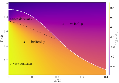
Figure 2: (Color online) A representative pairing phase diagram. The white solid line divides the pairing phase diagram into two regions, with one favoring the mixed $s+\text{helical}\,p$-wave pairing and the other favoring the mixed $s+\text{chiral}\,p$-wave pairing. The former preserves the $\mathcal{C}_{4z}\mathcal{T}$ symmetry, while the latter does not. Below the black dashed line, along which $|\Delta_{\uparrow\downarrow}^{s}|=|\Delta_{\uparrow\uparrow}^{p+}|$, is a sizable region with dominant helical $p$-wave pairing. Here the parameters are $t=0.5$, $t_{\rm AM}=0.1$, $\mu=-1$ and $V_{p}=1.5$.

Both types of the pairing solutions are found in the same parameter space and so we need to compare their corresponding condensation energies to determine the pairing ground state. The resulting pairing phase diagram takes the generic structure shown in Fig.2. We see that the superconductor favors a mixed $s+$ chiral $p$-wave pairing for strong RSOC and a mixed $s+$ helical $p$-wave pairing for weak RSOC. In the former phase, the $s$-wave component is always dominant, whereas in the latter the $p$-wave component can dominate over the $s$-wave one for a significant range of $V_{s}/V_{p}$. The $s$-wave dominant and the $p$-wave dominant pairings indeed regress to the pure $s$-wave and the pure $p$-wave pairings respectively in the $\lambda\rightarrow 0$ limit. However, in the case of pure $p$-wave pairing, chiral and helical $p$-wave pairings are completely degenerate.

The two phases in Fig. 2 are not only distinguished by the nature of the $p$-wave pairings but also by their different magnetic properties. Since the pairing amplitudes among spin up and spin down electrons are not equal for mixed chiral $p$-wave pairing, a finite net magnetization emerges in this phase. Thus, the fact that this phase is favored for strong RSOC is rather reminiscent of the charge-neutral atomic superfluid with SOC, where a strong SOC leads to chirality as well as finite magnetization Sun et al. (2018); Chen et al. (2023). Lastly, these two phases can also be differentiated by whether they preserves the $\mathcal{C}_{4z}\mathcal{T}$ symmetry. As we shall see immediately, this turns out to be very consequential for the topological properties of the superconducting phases.

II.3 Diverse topological superconducting phases

Based on the pairing phase diagram and the BdG Hamiltonian (5), we investigate possible topological superconducting phases. We begin with the $\lambda=0$ axis on the phase diagram, where only pure parity pairing occurs. Since the three possible pairings can be classified by symmetry properties, the first thing to note is that if the superconducting state possesses the $\mathcal{C}_{4z}\mathcal{T}$ symmetry it will forbid the presence of chiral TSC even though the TRS has been broken by AM. This fact can be intuitively recognized since in such a scenario two edges related by $\mathcal{C}_{4z}$ rotation will carry chiral Majorana modes with opposite chiralities due to the concomitant time-reversal operation, implying a zero net Chern number. This symmetry argument suggests that among the three possible pairings, only the chiral $p$-wave pairing, which breaks the $\mathcal{C}_{4z}\mathcal{T}$ symmetry of the normal state, can lead to the realization of chiral TSCs. For a chiral $p$-wave superconductor, the Chern number $C$ has a simple relation to the number of Fermi surfaces $N_{\rm FS}$ enclosing one time-reversal invariant momentum, i.e., $(-1)^{C}=(-1)^{N_{\rm FS}}$ Sato (2010). Since the zero net magnetization of the normal state in the AM metal demands an even ${N_{\rm FS}}$, an even Chern number is thus enforced. For example, we find $C=-2$ for the Fermi surface configuration shown in Fig.1(b).

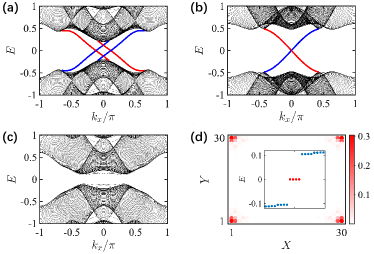
Figure 3: (Color online) (a) A chiral TSC with Chern number $C=-2$. The blue and red solid lines refer to chiral Majorana modes on two opposite edges. (b) A helical TSC with a pair of helical Majorana modes. The blue and red solid lines are doubly degenerate. (c)-(d) A second-order TSC with gapped edge spectra and four Majorana corner modes. The four red dots in the inset of (d) refers to four Majorana zero modes, with their probability density profiles concentrating around the four corners. Common parameters are $t=0.5$, $t_{\rm AM}=0.1$, and $\mu=-1$. The rest of parameters are as follows. (a) $\lambda=0.2$, $\Delta_{\uparrow\downarrow}^{s}=0.05$, and $\Delta_{\uparrow\uparrow}^{p+}=\Delta_{\downarrow\downarrow}^{p+}=0.25$ for the chiral $p$-wave pairing amplitude; (b) $\lambda=0$, $\Delta_{\uparrow\downarrow}^{s}=0$; (c)-(d) $\lambda=0.2$, $\Delta_{\uparrow\downarrow}^{s}=0.05$. In (b)-(d), the helical $p$-wave pairing amplitude is chosen to be $\Delta_{\uparrow\uparrow}^{p+}=0.25$.

We focus on the chiral $p$-wave pairing for the moment and move into regions of finite $\lambda$ in the phase diagram, where the pairings are now mixed with an $s$-wave component. In this case, whether such a mixed-parity superconducting phase supports a chiral TSC hinges on the relative weight between the two pairing components. When the $s$-wave component dominates, the superconducting phase is topologically trivial since it is adiabatically connected to the pure $s$-wave limit with $\mathcal{C}_{4z}\mathcal{T}$ symmetry as long as the bulk gap remains open. Similarly, when the chiral $p$-wave pairing dominates, the superconducting phase is adiabatically connected to the pure chiral $p$-wave limit and retains the topological properties of that limit. A calculation of the energy spectrum of a cylindrical sample shows the existence of two chiral Majorana modes on an open edge, also confirming the realization of a chiral TSC with $C=-2$ when the chiral $p$-wave pairing dominates, as shown in Fig.3(a). Due to the even $C$ constraint, this mixed chiral $p$-wave phase must transition directly to a trivial phase with $C=0$ when the $s$-wave component gradually increases.

Now let us turn to the helical $p$-wave pairing. In the $\lambda=0$ limit, we find that the superconductor with pure helical $p$-wave pairing supports helical Majorana modes protected by mirror symmetry $\mathcal{M}_{z}$ Teo et al. (2008); Feng et al. (2022b); Zhang et al. (2013b) or subsystem chiral symmetries Ryu et al. (2010); Zhu et al. (2023). An example is provided in Fig.3(b), where we show that the resulting superconductor carries a pair of helical Majorana modes on the boundary for a Fermi surface configuration shown in Fig.1(b). When the RSOC becomes finite, gapless Majorana modes are always absent, regardless of which component of the mixed $s+\text{helical}\,p$-wave pairing dominates, as exemplified in Fig.3(c). Despite being trivial in first-order topology, the superconductor is in fact a second-order TSC when the helical $p$-wave pairing dominates. Indeed, considering a square sample with open boundary conditions in both $x$ and $y$ directions, we find the hallmark of a second-order TSC, the existence of Majorana corner modes Langbehn et al. (2017); Geier et al. (2018); Khalaf (2018); Zhu (2018); Yan et al. (2018); Wang et al. (2018a, b), as shown in Fig.3(d).

The arising of a second-order TSC in the region with dominant helical $p$-wave pairing can also be understood via adiabatic and symmetry arguments. As mentioned above the helical Majorana modes in the $\lambda=0$ limit are protected by the mirror symmetry $\mathcal{M}_{z}$ or subsystem chiral symmetries (see Appendix C). However, all these symmetry protections are removed once $\lambda$ becomes finite, giving rise to a Dirac mass on the boundary to gap out the helical Majorana modes. On the other hand, the $\mathcal{C}_{4z}\mathcal{T}$ symmetry is retained in this mixed parity superconductor, which forces the Dirac masses on two nearby $\mathcal{C}_{4z}$-related edges to be opposite, and hence leads to the emergence of Majorana corner modes according to the Jackiw-Rebbi theory Jackiw and Rebbi (1976); this is very reminiscent of the scenario for the $\mathcal{C}_{4z}\mathcal{T}$ symmetry-enforced second-order topological insulator in 3D Schindler et al. (2018). A rather unique property of this symmetry-enforced second-order TSC is that the spin polarization of the four Majorana corner modes are entangled. That is, owing to the constraint from the $\mathcal{C}_{4z}\mathcal{T}$ symmetry, their out-of-plane spin polarizations will form a quadrupole structure Plekhanov et al. (2021), and the in-plane spin polarization will form a four-hour-clock-like structure. In experiments, such entangled structures of spin polarization can be detected by spin-polarized scanning tunneling microscopes as a defining signature of this second-order TSC He et al. (2014); Sun et al. (2016); Jeon et al. (2017).

III Discussions and conclusions

We have investigated the basic question of what kind of superconductivity and TSCs may emerge in 2D AM metals. A set of important symmetries relevant to the 2D AM metal with RSOC are unveiled, which place various constraints on the band structure, spin textures, and the pairing types for the realization of TSCs. Guided by the symmetry analysis, we have shown that the AM metal favors mixed parity pairings, and a multitude of TSCs, including both first-order and second-order TSCs, can emerge when the spin-triplet $p$-wave pairings dominate. We have also shown that the spin polarizations of Majorana corner modes on a square lattice take intriguing structures as the second-order TSC is enforced by the $\mathcal{C}_{4z}\mathcal{T}$ symmetry. All these findings prove that AM metals have unique band structures and can give birth to unconventional pairings and TSCs with fascinating properties.

Appendix A Chern metals driven by an out-of-plane magnetic field

By applying an out-of-plane magnetic field and only taking into account the resulting Zeeman-splitting effect, the Hamiltonian becomes

$$h(\boldsymbol{k}) = -2t(\cos k_{x}+\cos k_{y})\sigma_{0}+2t_{\rm AM}(\cos k_{x}-\cos k_{y})\sigma_{z}$$ (8)

$$+2\lambda(\sin k_{y}\sigma_{x}-\sin k_{x}\sigma_{y})+B_{z}\sigma_{z},$$

where the last term, $B_{z}\sigma_{z}$, denotes the Zeeman field. It is readily checked that the Zeeman field preserves the $\mathcal{C}_{4z}$ rotational symmetry but breaks the time-reversal symmetry, thereby breaking the combined $\mathcal{C}_{4z}\mathcal{T}$ symmetry. As a result, a nonzero Chern number becomes allowed.

For the two-band Hamiltonian, the Berry curvature can be simply determined by the following formula Qi et al. (2006)

$$\Omega_{\pm}(\boldsymbol{k})=\pm\frac{\boldsymbol{d}(\boldsymbol{k})\cdot(\partial_{k_{x}}\boldsymbol{d}(\boldsymbol{k})\times\partial_{k_{y}}\boldsymbol{d}(\boldsymbol{k}))}{2d^{3}(\boldsymbol{k})}$$ (9)

where $\pm$ refer to the upper and lower band respectively, $\boldsymbol{d}(\boldsymbol{k})=(2\lambda\sin k_{y},-2\lambda\sin k_{x},B_{z}+2t_{\rm AM}(\cos k_{x}-\cos k_{y}))$, and $d(\boldsymbol{k})=|\boldsymbol{d}(\boldsymbol{k})|$. A straightforward calculation gives

$$\Omega_{\pm}(\boldsymbol{k})=\pm\frac{2\lambda^{2}[B_{z}\cos k_{x}\cos k_{y}-2t_{\rm AM}(\cos k_{x}-\cos k_{y})]}{d^{3}(\boldsymbol{k})}.$$

In the limit of $B_{z}=0$, the Berry curvature has the property $\Omega_{\pm}(k_{x},k_{y})=-\Omega_{\pm}(k_{y},-k_{x})$, also implying that the Chern number, which is the integral of the Berry curvature over the Brillouin zone, identically vanishes. For a finite $B_{z}$, a calculation of the Chern number yields

$$C_{\pm} = \frac{1}{2\pi}\int_{BZ}\Omega_{\pm}(\boldsymbol{k})d^{2}k$$ (13)

$$= \pm\left\{\begin{array}[]{cc}sgn(B_{z}t_{\rm AM}),&0<|B_{z}|<4|t_{\rm AM}|,\\ 0,&|B_{z}|>4|t_{\rm AM}|.\end{array}\right.$$

This result shows that an arbitrarily small out-of-plane magnetic field will open a gap to the spectrum, and renders a nonzero Chern number to the bands. In addition, it is easy to see from Eq.(13) that a reversal of the magnetic field’s direction will reverse the Chern number of the two bands, indicating that the Hamiltonian (1) describes a critical metallic phase.

Appendix B The determination of pairing phase diagram

In this part, we provide more details on the determination of the pairing phase diagram. We consider density-density interactions between electrons and assume the existence of discrete translational symmetry. Accordingly, the interaction takes the generic form

$$\hat{H}_{int} = \frac{1}{2}\sum_{ij\sigma\sigma^{\prime}}V_{{\sigma\sigma^{\prime}}}(\boldsymbol{R}_{i}-\boldsymbol{R}_{j})n_{i\sigma}n_{j\sigma^{\prime}}$$ (14)

$$= \frac{1}{2N_{L}}\sum_{\boldsymbol{q}\sigma\sigma^{\prime}}V_{{\sigma\sigma^{\prime}}}(\boldsymbol{q})n_{\boldsymbol{q}\sigma}n_{-\boldsymbol{q}\sigma^{\prime}},$$

where $\boldsymbol{R}_{i}$ is the lattice site, $N_{L}$ is the total number of sites,

$$n_{\boldsymbol{q}\sigma}=\sum_{i}n_{i\sigma}e^{-i\boldsymbol{q}\cdot\boldsymbol{R}_{i}}=\sum_{\boldsymbol{k}}c^{\dagger}_{\boldsymbol{k}\sigma}c_{\boldsymbol{k}-\boldsymbol{q}\sigma},$$ (15)

and

$$V_{{\sigma\sigma^{\prime}}}(\boldsymbol{q}) = \sum_{j}V_{{\sigma\sigma^{\prime}}}(\boldsymbol{R}_{i}-\boldsymbol{R}_{j})e^{-i\boldsymbol{q}\cdot(\boldsymbol{R}_{i}-\boldsymbol{R}_{j})}$$ (16)

$$= V_{{\sigma\sigma^{\prime}}}(-\boldsymbol{q}).$$

For the last equation, we have used the property $V_{{\sigma\sigma^{\prime}}}(\boldsymbol{R}_{i}-\boldsymbol{R}_{j})=V_{{\sigma\sigma^{\prime}}}(\boldsymbol{R}_{j}-\boldsymbol{R}_{i})$.

Following the Bardeen-Cooper-Schrieffer (BCS) theory, the pairing interaction is simplified as

$$\hat{H}_{int}\approx\frac{1}{2}\sum_{\boldsymbol{k}\sigma\sigma^{\prime}}\Xi_{\sigma\sigma^{\prime}}(\boldsymbol{k})c^{\dagger}_{\boldsymbol{k}\sigma}c^{\dagger}_{-\boldsymbol{k}\sigma^{\prime}}+h.c.,$$ (17)

where the gap function is defined as

$$\Xi_{\sigma\sigma^{\prime}}(\boldsymbol{k})=-\frac{1}{N_{L}}\sum_{\boldsymbol{k}^{\prime}}V_{{\sigma\sigma^{\prime}}}(\boldsymbol{k}-\boldsymbol{k}^{\prime})\langle c_{\boldsymbol{k}^{\prime}\sigma}c_{-\boldsymbol{k}^{\prime}\sigma^{\prime}}\rangle.$$ (18)

Fermi statistics and the fact that $V_{\sigma\sigma^{\prime}}(\boldsymbol{q})=V_{\sigma^{\prime}\sigma}(-\boldsymbol{q})$ lead to the following property of the gap function,

$$\Xi_{\sigma\sigma^{\prime}}(\boldsymbol{k})=-\Xi_{\sigma^{\prime}\sigma}(-\boldsymbol{k}).$$ (19)

To determine possible pairing channels, one may expand $V_{\sigma\sigma^{\prime}}({\boldsymbol{k}-\boldsymbol{k}^{\prime}})$ in terms of the so-called square lattice harmonics $g_{\eta}(\boldsymbol{k})$

$$V_{\sigma\sigma^{\prime}}({\boldsymbol{k}-\boldsymbol{k}^{\prime}})=\sum_{\eta}\gamma^{\eta}_{\sigma\sigma^{\prime}}g_{\eta}(\boldsymbol{k})g_{\eta}^{*}(\boldsymbol{k}^{\prime}),$$ (20)

where $\gamma^{\eta}_{\sigma\sigma^{\prime}}$ is the strength of the pairing interaction in the $\eta$-channel. Examples of the harmonics include the $s$-wave $g_{s}(\boldsymbol{k})=1$, the extended $s$-wave $g_{es}(\boldsymbol{k})=\cos k_{x}+\cos k_{y}$, the $p$-waves $g_{p\pm}(\boldsymbol{k})=\sin k_{x}\pm i\sin k_{y}$ and the $d$-wave $g_{d}(\boldsymbol{k})=\cos k_{x}-\cos k_{y}$. The gap function can similarly be written as

$$\Xi_{\sigma\sigma^{\prime}}(\boldsymbol{k})=\sum_{\eta}\Delta_{\sigma\sigma^{\prime}}^{\eta}g_{\eta}(\boldsymbol{k}).$$ (21)

Substituting Eq. (21) into Eq. (18), we obtain the amplitudes of each pairing channel as

$$\Delta_{\sigma\sigma^{\prime}}^{\eta}=-\frac{1}{N_{L}}\sum_{\boldsymbol{k}^{\prime}}\gamma^{\eta}_{\sigma\sigma^{\prime}}g_{\eta}^{*}(\boldsymbol{k}^{\prime})\langle c_{\boldsymbol{k}^{\prime}\sigma}c_{-\boldsymbol{k}^{\prime}\sigma^{\prime}}\rangle.$$ (22)

Introducing the Nambu basis $\Psi_{\boldsymbol{k}}=(c_{\boldsymbol{k}\uparrow},c_{\boldsymbol{k}\downarrow},c^{\dagger}_{-\boldsymbol{k}\uparrow},c^{\dagger}_{-\boldsymbol{k}\downarrow})^{T}$, the BCS Hamiltonian can be written as

$$\hat{H}-\mu\hat{N}=\frac{1}{2}\sum_{\boldsymbol{k}}\Psi^{\dagger}_{\boldsymbol{k}}\mathcal{H}_{\rm BdG}(\boldsymbol{k})\Psi_{\boldsymbol{k}},$$ (23)

with

$$\mathcal{H}_{\rm BdG}(\boldsymbol{k})=\begin{bmatrix}\xi_{\boldsymbol{k}\uparrow}&\Lambda(\boldsymbol{k})&\Xi_{\uparrow\uparrow}(\boldsymbol{k})&\Xi_{\uparrow\downarrow}(\boldsymbol{k})\\ \Lambda^{*}(\boldsymbol{k})&\xi_{\boldsymbol{k}\downarrow}&\Xi_{\downarrow\uparrow}(\boldsymbol{k})&\Xi_{\downarrow\downarrow}(\boldsymbol{k})\\ \Xi^{*}_{\uparrow\uparrow}(\boldsymbol{k})&\Xi^{*}_{\downarrow\uparrow}(\boldsymbol{k})&-\xi_{\boldsymbol{k}\uparrow}&-\Lambda^{*}(-\boldsymbol{k})\\ \Xi^{*}_{\uparrow\downarrow}(\boldsymbol{k})&\Xi^{*}_{\downarrow\downarrow}(\boldsymbol{k})&-\Lambda(-\boldsymbol{k})&-\xi_{\boldsymbol{k}\downarrow}\end{bmatrix},$$ (24)

where

$$\xi_{\boldsymbol{k}\uparrow} =-2(t-t_{\rm AM})\cos k_{x}-2(t+t_{\rm AM})\cos k_{y}-\mu,$$

$$\xi_{\boldsymbol{k}\downarrow} =-2(t+t_{\rm AM})\cos k_{x}-2(t-t_{\rm AM})\cos k_{y}-\mu,$$

$$\Lambda(\boldsymbol{k}) =2\lambda(\sin k_{y}+i\sin k_{x}).$$ (25)

The above Hamiltonian can be diagonalized by the following Bogoliubov transformation

$$c_{\boldsymbol{k}\sigma} = u_{\sigma,1}(\boldsymbol{k})b_{\boldsymbol{k},1}+v_{\sigma,1}^{*}(-\boldsymbol{k})b^{\dagger}_{-\boldsymbol{k},1}$$ (26)

$$+u_{\sigma,2}(\boldsymbol{k})b_{\boldsymbol{k},2}+v_{\sigma,2}^{*}(-\boldsymbol{k})b^{\dagger}_{-\boldsymbol{k},2},$$

where $u_{\sigma,l},v_{\sigma,l}$ with $l=\{1,2\}$ are the Bogoliubov amplitudes and $b_{\boldsymbol{k},l}$ refer to the two quasiparticle operators. The Bogoliubov amplitudes are obtained from the eigenvalue equation

$$\mathcal{H}_{\rm BdG}(\boldsymbol{k})\chi_{\boldsymbol{k},l}=E_{\boldsymbol{k},l}\chi_{\boldsymbol{k},l},$$ (27)

where $E_{\boldsymbol{k},l}$ refer to the two positive eigenenergies, and $\chi_{\boldsymbol{k},l}\equiv[u_{\uparrow,l}(\boldsymbol{k}),u_{\downarrow,l}(\boldsymbol{k}),v_{\uparrow,l}(\boldsymbol{k}),v_{\downarrow,l}(\boldsymbol{k})]^{T}$ are the corresponding eigenstates. Using Eq. (26), the gap equation (22) can be written as

$$\Delta_{\sigma\sigma^{\prime}}^{\eta} = -\frac{1}{N_{L}}\sum_{\boldsymbol{k}}\gamma_{\sigma\sigma^{\prime}}^{\eta}g^{*}_{\eta}(\boldsymbol{k})$$ (28)

$$\times\left[u_{\sigma,1}(\boldsymbol{k})v_{\sigma^{\prime},1}^{*}(\boldsymbol{k})+u_{\sigma,2}(\boldsymbol{k})v_{\sigma^{\prime},2}^{*}(\boldsymbol{k})\right].$$

Once the gap functions are obtained, the free energy of the superconductor at zero temperature can be calculated as

$$F_{S} = -\frac{1}{2}\sum_{\boldsymbol{k}}[E_{\boldsymbol{k},+}+E_{\boldsymbol{k},-}-\xi_{\boldsymbol{k}\uparrow}-\xi_{\boldsymbol{k}\downarrow}]+\frac{1}{2}\sum_{\sigma\sigma^{\prime}{\boldsymbol{k}}}\Xi^{*}_{\sigma\sigma^{\prime}}(\boldsymbol{k})$$ (29)

$$\times\left[u_{\sigma,1}(\boldsymbol{k})v_{\sigma^{\prime},1}^{*}(\boldsymbol{k})+u_{\sigma,2}(\boldsymbol{k})v_{\sigma^{\prime},2}^{*}(\boldsymbol{k})\right].$$

The condensation energy is

$$\delta E=F_{S}-F_{N},$$ (30)

where $F_{N}$ is the free energy of the normal state

$$F_{N}=\sum_{\boldsymbol{k},\alpha=\pm}(\varepsilon_{\alpha}(\boldsymbol{k})-\mu)\theta(\mu-\varepsilon_{\alpha}(\boldsymbol{k})).$$ (31)

where the energy spectra $\varepsilon_{\pm}(\boldsymbol{k})=-2t(\cos k_{x}+\cos k_{y})\pm 2\sqrt{(t_{\rm AM}(\cos k_{x}-\cos k_{y}))^{2}+\lambda^{2}(\sin^{2}k_{x}+\sin^{2}k_{y})}$.

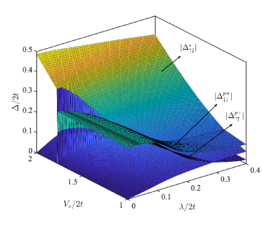
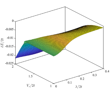
Figure 4: (color online) The $s+$ chiral $p$-wave solution of the gap equations . Here $t=0.5$, $t_{\rm AM}=0.1$, $V_{p}=1.5$, and $\mu=-1$. Left: the pairing amplitudes. Right: the condensation energy.

Now we turn to our specific short-range interaction (an extended attractive Hubbard interaction)

$$\hat{H}_{int}=-V_{s}\sum_{i}n_{i\uparrow}n_{i\downarrow}-V_{p}\sum_{\langle ij\rangle,\sigma}n_{i\sigma}n_{j\sigma}$$ (32)

for which

$$V_{\sigma\sigma^{\prime}}(\boldsymbol{q})=\left\{\begin{tabular}[]{cc}$-V_{s},$&\qquad$\sigma\neq\sigma^{\prime}$,\\ $-2V_{p}\left(\cos q_{x}+\cos q_{y}\right),$&\qquad$\sigma=\sigma^{\prime}$.\\ \end{tabular}\right.$$ (33)

In terms of $g_{\eta}(\boldsymbol{k})$, one finds

$$V_{\uparrow\downarrow}({\boldsymbol{k}-\boldsymbol{k}^{\prime}}) = V_{\downarrow\uparrow}({\boldsymbol{k}-\boldsymbol{k}^{\prime}})=-V_{s}g_{s}(\boldsymbol{k})g^{*}_{s}(\boldsymbol{k}^{\prime}),$$

$$V_{\uparrow\uparrow}({\boldsymbol{k}-\boldsymbol{k}^{\prime}}) = V_{\downarrow\downarrow}({\boldsymbol{k}-\boldsymbol{k}^{\prime}})=-V_{p}\left[g_{es}(\boldsymbol{k})g^{*}_{es}(\boldsymbol{k}^{\prime})+g_{d}(\boldsymbol{k})g^{*}_{d}(\boldsymbol{k}^{\prime})+g_{p+}(\boldsymbol{k})g^{*}_{p+}(\boldsymbol{k}^{\prime})+g_{p-}(\boldsymbol{k})g^{*}_{p-}(\boldsymbol{k}^{\prime})\right].$$ (34)

It is worth mentioning that, in the above decomposition, $V_{\uparrow\uparrow}$ and $V_{\downarrow\downarrow}$ not only contain $p$-wave harmonic components, but also contain extended $s$-wave and $d$-wave harmonic components. However, because this attractive interaction occurs between electrons with the same spin, it can not result in extended $s$-wave pairing or $d$-wave pairing due to the Fermi statistics. As extended $s$-wave and $d$-wave pairings are spin singlet, their formation requires an attractive interaction between two electrons possessing opposite spins and located at two nearest-neighbor sites, i.e., $-V_{sd}\sum_{\langle ij\rangle}n_{i\uparrow}n_{j\downarrow}$. To have pairings with even higher angular momentum, such as an $f$-wave spin-triplet pairing, one needs to further consider longer-range attractive interactions, such as the next-nearest-neighbor attractive interaction. In this work, to have a neat understanding of the pairing phase diagram and the potential topological superconducting phases, we will focus on the simple interaction given in Eq.(32). Accordingly, only on-site $s$-wave pairing and $p$-wave pairing will show up. Despite focusing on this simple interaction, we would like to emphasize that it is sufficient to capture all key physics, including the competition of even-parity and odd-parity pairings in an inversion-asymmetric system, and all possible topological superconducting phases at a qualitative level. In the following, we explain how we determine the superconducting ground state and the pairing phase diagram.

As a result of the pairing interaction and the symmetry property of the gap function in Eq. (19), we have

$$\Xi_{\uparrow\downarrow}(\boldsymbol{k}) =-\Xi_{\downarrow\uparrow}(\boldsymbol{k})=\Delta^{s}_{\uparrow\downarrow},$$

$$\Xi_{\uparrow\uparrow}(\boldsymbol{k}) =\Delta^{p+}_{\uparrow\uparrow}g_{p+}(\boldsymbol{k})+\Delta^{p-}_{\uparrow\uparrow}g_{p-}(\boldsymbol{k}),$$

$$\Xi_{\downarrow\downarrow}(\boldsymbol{k}) =\Delta^{p+}_{\downarrow\downarrow}g_{p+}(\boldsymbol{k})+\Delta^{p-}_{\downarrow\downarrow}g_{p-}(\boldsymbol{k}).$$ (35)

The general forms of $\Xi_{\uparrow\uparrow}(\boldsymbol{k})$ and $\Xi_{\downarrow\downarrow}(\boldsymbol{k})$ do not necessarily preserve the lattice symmetry. The two types of solutions that do are: (i) chiral $p$-wave with $(\Xi_{\uparrow\uparrow}(\boldsymbol{k}),\Xi_{\downarrow\downarrow}(\boldsymbol{k}))=(\Delta^{p+}_{\uparrow\uparrow}g_{p+}(\boldsymbol{k}),\Delta^{p+}_{\downarrow\downarrow}g_{p+}(\boldsymbol{k}))$ or $(\Xi_{\uparrow\uparrow}(\boldsymbol{k}),\Xi_{\downarrow\downarrow}(\boldsymbol{k}))=(\Delta^{p-}_{\uparrow\uparrow}g_{p-}(\boldsymbol{k}),\Delta^{p-}_{\downarrow\downarrow}g_{p-}(\boldsymbol{k}))$; and (ii) helical $p$-wave with $(\Xi_{\uparrow\uparrow}(\boldsymbol{k}),\Xi_{\downarrow\downarrow}(\boldsymbol{k}))=(\Delta^{p+}_{\uparrow\uparrow}g_{p+}(\boldsymbol{k}),\Delta^{p-}_{\downarrow\downarrow}g_{p-}(\boldsymbol{k}))$ or $(\Xi_{\uparrow\uparrow}(\boldsymbol{k}),\Xi_{\downarrow\downarrow}(\boldsymbol{k}))=(\Delta^{p-}_{\uparrow\uparrow}g_{p-}(\boldsymbol{k}),\Delta^{p+}_{\downarrow\downarrow}g_{p+}(\boldsymbol{k}))$. It is noteworthy that for the chiral $p$-wave pairing, the two situations, $(\Xi_{\uparrow\uparrow},\Xi_{\downarrow\downarrow})=(\Delta^{p+}_{\uparrow\uparrow}g_{p+},\Delta^{p+}_{\downarrow\downarrow}g_{p+})$ and $(\Xi_{\uparrow\uparrow},\Xi_{\downarrow\downarrow})=(\Delta^{p-}_{\uparrow\uparrow}g_{p-},\Delta^{p-}_{\downarrow\downarrow}g_{p-})$, lead to the same condensation energy and similar topological property for the superconducting phase (only the sign of the Chern number will be different since the pairings for the two cases carry opposite angular momentum). For this reason we only discuss the case of $(\Xi_{\uparrow\uparrow},\Xi_{\downarrow\downarrow})=(\Delta^{p+}_{\uparrow\uparrow}g_{p+},\Delta^{p+}_{\downarrow\downarrow}g_{p+})$. For the helical $p$-wave pairing, similarly, the two situations, $(\Xi_{\uparrow\uparrow},\Xi_{\downarrow\downarrow})=(\Delta^{p+}_{\uparrow\uparrow}g_{p+},\Delta^{p-}_{\downarrow\downarrow}g_{p-})$ and $(\Xi_{\uparrow\uparrow},\Xi_{\downarrow\downarrow})=(\Delta^{p-}_{\uparrow\uparrow}g_{p-},\Delta^{p+}_{\downarrow\downarrow}g_{p+})$, lead to the same condensation energy and similar topological property for the superconducting phase, so we also only need to focus on one of the cases. Below, we focus on the case $(\Xi_{\uparrow\uparrow},\Xi_{\downarrow\downarrow})=(\Delta^{p+}_{\uparrow\uparrow}g_{p+},\Delta^{p-}_{\downarrow\downarrow}g_{p-})$. When both chiral $p$-wave pairing and helical $p$-wave pairing are solutions in the same parameter region, we need to compare their corresponding condensation energies in order to determine the ground state.

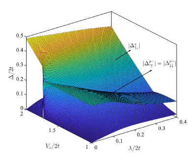
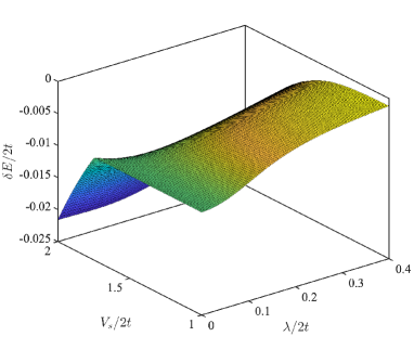
Figure 5: (color online) The $s+$ helical $p$-wave solution of the gap equations . Here $t=0.5$, $t_{\rm AM}=0.1$, $V_{p}=1.5$, and $\mu=-1$. Left: the pairing amplitudes. Right: the condensation energy.

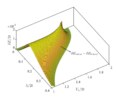
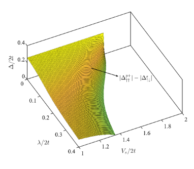
Figure 6: (color online) Left: the difference between the $p$-wave pairing amplitude and the $s$-wave pairing amplitude for the $s+$ helical $p$ solutions (only positive differences are shown). Right: the difference of condensation energies for the $s+$ chiral $p$-wave and the $s+$ helical $p$-wave solutions (only positive differences are shown).

When the Rashba spin-orbit coupling is absent, we find that the pairing has definitive parity, i.e., either even-parity or odd-parity. Whether the ground state favors the even-parity spin-singlet $s$-wave pairing or the odd-parity spin-triplet $p$-wave pairing naturally depends on the relative strength of $V_{s}$ and $V_{p}$. It turns out that helical $p$-wave and chiral $p$-wave pairings are degenerate in ground-state energy in the limit $\lambda=0$. If both $t_{\rm AM}$ and the spin-orbit coupling constant $\lambda$ are finite, we find that the general solution is a coexistence of $s$-wave and $p$-wave pairings (either chiral or helical); in other words pure $s$-wave or pure $p$-wave pairings are absent when the Rashba spin-orbit coupling enters. In Fig. 4 (left) and (right) we show respectively the pairing amplitudes and the condensation energy for the solution of mixed $s+$ chiral $p$-wave pairing. We note that the two $p$-wave pairing amplitudes, $\Delta^{p+}_{\uparrow\uparrow}$ and $\Delta^{p+}_{\downarrow\downarrow}$, are the same in magnitude when the spin-orbit coupling $\lambda$ is absent but they begin to gradually deviate as $\lambda$ increases. In Fig. 5 (left) and (right) we show respectively the pairing amplitudes and the condensation energy for the solution of mixed $s+$ helical $p$-wave pairing. In contrast to the chiral solutions, the two $p$-wave pairing amplitudes, $\Delta^{p+}_{\uparrow\uparrow}$ and $\Delta^{p-}_{\downarrow\downarrow}$, are always the same so that the net angular momentum of this superconducting state is zero.

The phase diagram in the main text is obtained by first comparing the condensation energies of the $s+$ chiral $p$-wave and the $s+$ helical $p$-wave pairing solutions. Shown in Fig. 6 (left) is $\delta E_{chiral}-\delta E_{helical}$ in the region where it is positive, namely in the region where the $s+$ helical $p$-wave pairing is the ground state. This region can be further divided into one where the $p$-wave pairing is dominant and one where $s$-wave pairing is dominant, by a direct comparison of the pairing amplitudes. Shown in Fig. 6 (right) is $|\Delta^{p}_{\uparrow\uparrow}|-|\Delta_{\uparrow\downarrow}^{s}|$ in the region where it is positive. The phase diagram is then straightforwardly determined from the two plots in Fig. 6.

Appendix C Topological properties of the superconducting phase with mixed $s+\text{helical}\,p$-wave pairing

When the pairing is a mixture of $s$-wave pairing and helical $p$-wave pairing, the BdG Hamiltonian is given by

$$\mathcal{H}_{\rm BdG}(\boldsymbol{k}) = [-2t(\cos k_{x}+\cos k_{y})-\mu]\tau_{z}\sigma_{0}$$ (36)

$$+2t_{\rm AM}(\cos k_{x}-\cos k_{y})\tau_{z}\sigma_{z}$$

$$+2\lambda(\sin k_{y}\tau_{0}\sigma_{x}-\sin k_{x}\tau_{z}\sigma_{y})$$

$$+2\Delta^{p}(\sin k_{x}\tau_{x}\sigma_{z}-\sin k_{y}\tau_{y}\sigma_{0})$$

$$+\Delta_{\uparrow\downarrow}^{s}\tau_{y}\sigma_{y},$$

where $\Delta_{\uparrow\uparrow}^{p+}=-\Delta_{\downarrow\downarrow}^{p-}=\Delta^{p}$ is set for notational simplicity. In this section, we give a detailed discussion about the symmetry protection of the topological superconducting phase in the $\lambda=0$ limit. When $\lambda=0$, our numerical calculations in fact show that the pairing has fixed parity for the investigated parameter region. Here for a generic discussion of the symmetry protection of the band topology we ignore this parity constraint and still assume that the $s$-wave and helical $p$-wave pairings can coexist even in the $\lambda=0$ limit.

We first consider the $\Delta_{\uparrow\downarrow}^{s}=0$ limit. For this case, the BdG Hamiltonian (36) reduces to

$$\mathcal{H}_{\rm p}(\boldsymbol{k}) = [-2t(\cos k_{x}+\cos k_{y})-\mu]\tau_{z}\sigma_{0}$$ (37)

$$+2t_{\rm AM}(\cos k_{x}-\cos k_{y})\tau_{z}\sigma_{z}$$

$$+2\Delta^{p}(\sin k_{x}\tau_{x}\sigma_{z}-\sin k_{y}\tau_{y}\sigma_{0}).$$

This reduced Hamiltonian has mirror symmetry $\mathcal{M}_{z}$, i.e., $\mathcal{M}_{z}\mathcal{H}_{\rm p}(\boldsymbol{k})\mathcal{M}_{z}^{-1}=\mathcal{H}_{\rm p}(\boldsymbol{k})$ with $\mathcal{M}_{z}=i\tau_{0}\sigma_{z}$. According to the two possible eigenvalues of $\mathcal{M}_{z}$, i.e., $\pm i$, the Hamiltonian can be decomposed as $\mathcal{H}_{\rm p}(\boldsymbol{k})=\mathcal{H}_{i}(\boldsymbol{k})\oplus\mathcal{H}_{-i}(\boldsymbol{k})$, where $\mathcal{H}_{\pm i}(\boldsymbol{k})=\boldsymbol{d}_{\pm i}(\boldsymbol{k})\cdot\boldsymbol{\tau}$ with

$$\boldsymbol{d}_{i}(\boldsymbol{k}) = (2\Delta^{p}\sin k_{x},-2\Delta^{p}\sin k_{y},\xi_{\boldsymbol{k}\uparrow}),$$

$$\boldsymbol{d}_{-i}(\boldsymbol{k}) = (2\Delta^{p}\sin k_{x},-2\Delta^{p}\sin k_{y},\xi_{\boldsymbol{k}\downarrow}).$$ (38)

Each sector is a chiral $p$-wave superconductor and is accordingly characterized by a Chern number. The Chern numbers characterizing the two mirror-graded Hamiltonians are simply given by Qi et al. (2006)

$$C_{\pm i}=-\frac{1}{4\pi}\int_{BZ}\frac{\boldsymbol{d}_{\pm i}\cdot[\partial_{k_{x}}\boldsymbol{d}_{\pm i}\times\partial_{k_{y}}\boldsymbol{d}_{\pm i}]}{d_{\pm i}^{3}}d^{2}k,$$ (39)

where $d_{\pm i}=|\boldsymbol{d}_{\pm i}|$ denotes the norm of the $\boldsymbol{d}_{\pm i}$ vector. Without loss of generality, we take $t>t_{\rm AM}>0$. Then a straightforward calculation yields

$$C_{i}=-C_{-i}=\left\{\begin{array}[]{cc}0,&\mu>4t,\\ 1,&4t_{\rm AM}<\mu<4t,\\ 0,&-4t_{\rm AM}<\mu<4t_{\rm AM},\\ -1,&-4t<\mu<-4t_{\rm AM},\\ 0,&\mu<-4t.\end{array}\right.$$ (45)

The result suggests that the total Chern number, which is given by the sum of the two mirror-graded Chern numbers, is always zero. We have previously explained that this is a natural result due to the constraint from the $\mathcal{C}_{4z}\mathcal{T}$ symmetry. Although the total Chern number is zero, the mirror Chern number, which is defined as $C_{M}=(C_{i}-C_{-i})/2$ Teo et al. (2008), has an absolute value of $1$ when $4t_{\rm AM}<|\mu|<4t$. When $|C_{M}|=1$, the superconducting phase is a topological mirror superconductor with a pair of helical Majorana modes on the open edges Zhang et al. (2013b).

When $\Delta_{\uparrow\downarrow}^{s}$ is nonzero, the Hamiltonian becomes

$$\mathcal{H}_{\rm sp}(\boldsymbol{k}) = [-2t(\cos k_{x}+\cos k_{y})-\mu]\tau_{z}\sigma_{0}$$ (46)

$$+2t_{\rm AM}(\cos k_{x}-\cos k_{y})\tau_{z}\sigma_{z}$$

$$+2\Delta^{p}(\sin k_{x}\tau_{x}\sigma_{z}-\sin k_{y}\tau_{y}\sigma_{0})$$

$$+\Delta_{\uparrow\downarrow}^{s}\tau_{y}\sigma_{y}.$$

Since the $s$-wave pairing term anticommutes with the mirror symmetry operator, i.e., $\{\Delta_{\uparrow\downarrow}^{s}\tau_{y}\sigma_{y},i\tau_{0}\sigma_{z}\}=0$, the mirror symmetry is broken. Without the protection of mirror symmetry, the helical Majorana edge modes are expected to be gapped due to potential hybridization. However, we find that the helical Majorana edge modes remain robust, suggesting that there exists some additional symmetry protection. This can be seen as follows. From the view point of dimensional reduction, we may view the momentum for the direction with periodic boundary conditions as a tuning parameter. Then the spectrum crossing of the helical Majorana edge modes suggests that the one-dimensional Hamiltonian is a topological superconductor with two Majorana zero modes at each boundary. To be more specific, let us take $k_{x}$ as a tuning parameter. We can then view the two-dimensional Hamiltonian as a one-dimensional parameter-dependent Hamiltonian $\mathcal{H}_{k_{x}}(k_{y})$. Now only the argument $k_{y}$ in the bracket has the meaning as a momentum. For this parameter-dependent Hamiltonian $\mathcal{H}_{k_{x}}(k_{y})$, one finds that the Hamiltonian has an emergent chiral symmetry at $k_{x}=0$ and $k_{x}=\pi$, i.e., $\{\mathcal{C},\mathcal{H}_{k_{x}}(k_{y})\}=0$. The explicit form of the chiral symmetry operator is $\mathcal{C}=\tau_{x}\sigma_{0}$. The existence of chiral symmetry suggests that a winding number can be assigned to characterize the band topology of $\mathcal{H}_{0}(k_{y})$ and $\mathcal{H}_{\pi}(k_{y})$ Ryu et al. (2010). To determine the winding number, the first step is to rewrite the Hamiltonian by changing the original basis to a new one in which the chiral symmetry operator takes a diagonal form, i.e., $\tilde{\mathcal{C}}=\tau_{z}\sigma_{0}$. Apparently, this can be realized by a unitary operation of the form $U=e^{i\pi\tau_{y}\sigma_{0}/4}$, i.e., $U\mathcal{C}U^{-1}=\tilde{\mathcal{C}}$. In the new basis, the form of the Hamiltonian becomes off-diagonal. Let us take $\mathcal{H}_{0}(k_{y})$ as a specific example. It is straightforward to find

$$U\mathcal{H}_{0}(k_{y})U^{-1}=\left(\begin{array}[]{cc}0&Q_{0}(k_{y})\\ Q_{0}^{{\dagger}}(k_{y})&0\\ \end{array}\right),$$ (49)

where $Q_{0}(k_{y})$ is a two-by-two matrix of the form

$$Q_{0}(k_{y})=\left(\begin{array}[]{cc}q_{-}(k_{y})&-\Delta_{\uparrow\downarrow}^{s}\\ \Delta_{\uparrow\downarrow}^{s}&q_{+}(k_{y})\\ \end{array}\right),$$ (52)

where $q_{\pm}(k_{y})=[2(t\pm t_{\rm AM})+\mu+2(t\mp t_{\rm AM})\cos k_{y}]+2i\Delta^{p}\sin k_{y}$. The winding number is given by Ryu et al. (2010)

$$W_{0}=\frac{i}{2\pi}\int_{-\pi}^{\pi}\text{Tr}[Q_{0}^{-1}(k_{y})\partial_{k_{y}}Q_{0}(k_{y})]dk_{y}.$$ (54)

The winding number $W_{0}$ also does not change its value as long as the energy gap of $\mathcal{H}_{0}(k_{y})$ remains open. Again let us first focus on the limiting case of $\Delta_{\uparrow\downarrow}^{s}=0$, for which $Q_{0}(k_{y})$ is diagonal, i.e.,

$$Q_{0}(k_{y})=\left(\begin{array}[]{cc}q_{-}(k_{y})&0\\ 0&q_{+}(k_{y})\\ \end{array}\right).$$ (57)

Accordingly, it is easy to find that

$$W_{0}=W_{0}^{(-)}+W_{0}^{(+)},$$ (58)

where

$$W_{0}^{(\pm)}=\frac{i}{2\pi}\int_{-\pi}^{\pi}[q_{\pm}^{-1}(k_{y})\partial_{k_{y}}q_{\pm}(k_{y})]dk_{y}.$$ (59)

A straightforward calculation yields

$$W_{0}^{(-)}=\left\{\begin{array}[]{cc}0,&\mu>4t_{\rm AM},\\ -1,&-4t<\mu<4t_{\rm AM},\\ 0,&\mu<-4t,\end{array}\right.$$ (63)

and

$$W_{0}^{(+)}=\left\{\begin{array}[]{cc}0,&\mu>-4t_{\rm AM},\\ -1,&-4t<\mu<-4t_{\rm AM},\\ 0,&\mu<-4t.\end{array}\right.$$ (67)

Similar analysis shows that for $\mathcal{H}_{\pi}(k_{y})$ with $\Delta_{\uparrow\downarrow}^{s}=0$,

$$W_{\pi}^{(-)}=\left\{\begin{array}[]{cc}0,&\mu>4t,\\ -1,&-4t_{\rm AM}<\mu<4t,\\ 0,&\mu<-4t_{\rm AM},\end{array}\right.$$ (71)

and

$$W_{\pi}^{(+)}=\left\{\begin{array}[]{cc}0,&\mu>4t,\\ -1,&4t_{\rm AM}<\mu<4t,\\ 0,&\mu<4t_{\rm AM}.\end{array}\right.$$ (75)

Based on the above analysis, we reach the following result,

$$(W_{0},W_{\pi})=\left\{\begin{array}[]{cc}(0,0),&\mu>4t,\\ (0,-2),&4t_{\rm AM}<\mu<4t,\\ (-1,-1),&-4t_{\rm AM}<\mu<4t_{\rm AM},\\ (-2,0),&-4t<\mu<-4t_{\rm AM},\\ (0,0),&\mu<-4t.\end{array}\right.$$ (81)

Comparing with the mirror Chern number, we see that $C_{M}=1$ and $C_{M}=-1$ correspond to $(W_{0},W_{\pi})=(-2,0)$ and $(0,-2)$, respectively. Obviously, the value $-2$ of the winding number also guarantees the robustness of the spectrum-crossing feature of the helical Majorana modes. Interestingly, using the winding number, we find that the superconducting phase is also topologically nontrivial in the region $-4t_{\rm AM}<\mu<4t_{\rm AM}$ even though the mirror Chern number is zero. In this region, the two winding numbers $W_{0}$ and $W_{\pi}$ both take value $1$. It means that if the translational symmetry is preserved in the $x$ direction, on each $y$-normal edge there are two branches of chiral Majorana modes with opposite chiralities, with one branch traversing the gap at $k_{x}=0$, and the other traversing the gap at $k_{x}=\pi$, as shown in Fig.7. This superconducting phase can be categorized as a weak topological superconducting phase as it is protected by topological invariants defined in noncontractible subspaces of the Brillouin zone. In this case whether the Majorana modes comes about relies on the orientation of the edges.

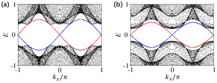
Figure 7: (color online) Common parameters are $t=0.5$, $t_{\rm AM}=0.1$, $\lambda=0.2$, $\mu=-0.0$ and $\Delta^{p}=0.25$. (a) $\Delta_{\uparrow\downarrow}^{s}=0.0$, (b) $\Delta_{\uparrow\downarrow}^{s}=0.2$. The red and blue solid lines refer to mid-gap states on opposite edges. The edge-state energy spectra tangentially touch with the bulk energy spectra when $\Delta_{\uparrow\downarrow}^{s}=0$, and become floating bands when $\Delta_{\uparrow\downarrow}^{s}$ becomes nonzero.

When $\Delta_{\uparrow\downarrow}^{s}$ becomes finite, the winding numbers retain their values as long as the energy gap remains open along those high symmetry lines. For the superconducting phase with $W_{0}=-2$ or $W_{\pi}=-2$, the robustness of the winding number explains the robust spectrum-crossing feature of the helical Majorana modes even when the mirror symmetry is broken by the mixture of $s$-wave and helical $p$-wave pairings. Due to the existence of $\mathcal{C}_{4z}\mathcal{T}$ symmetry, the physics is similar when the directions for the open boundary conditions and the periodic boundary conditions are reversed.

Below we provide a discussion on the condition for the change of winding number when $\Delta_{\uparrow\downarrow}^{s}$ is nonzero. Without loss of generality, we focus on the Hamiltonian $\mathcal{H}_{0}(k_{y})$ in Eq.(49) for a detailed discussion. The energy spectra of $\mathcal{H}_{0}(k_{y})$ can be analytically determined, which read

$$E(k_{y})=\pm\sqrt{h_{1}^{2}+h_{2}^{2}+h_{3}^{2}+h_{4}^{2}\pm 2\sqrt{h_{1}^{2}h_{2}^{2}+h_{2}^{2}h_{3}^{2}+h_{3}^{2}h_{4}^{2}}},$$

where $h_{1}=2t(1+\cos k_{y})+\mu$, $h_{2}=2t_{\rm AM}(1-\cos k_{y})$, $h_{3}=\Delta_{\uparrow\downarrow}^{s}$, and $h_{4}=2\Delta^{p}\sin k_{y}$. The band gap becomes closed when the parameters fulfill either one of the following two conditions,

$$(\text{I}):h_{4}=0,\quad h_{2}=\sqrt{h_{1}^{2}+h_{3}^{2}};$$

$$(\text{II}):h_{1}=0,\quad h_{3}=\sqrt{h_{2}^{2}+h_{4}^{2}}.$$ (83)

For case (I), if $\Delta_{\uparrow\downarrow}^{s}$ is nonzero, the band gap closes only at the time-reversal invariant momentum $k_{y}=\pi$ and only when $4t_{\rm AM}=\sqrt{(\Delta_{\uparrow\downarrow}^{s})^{2}+\mu^{2}}$. For case (II), the band gap closes at the momenta

$$k_{y}=\pm\left(\pi-\arccos\left(\frac{2t+\mu}{2t}\right)\right)$$ (84)

when

$$\Delta_{\uparrow\downarrow}^{s}=\sqrt{\frac{t_{\rm AM}^{2}\mu^{2}}{t^{2}}+\frac{(\Delta^{p})^{2}(\mu^{2}+4t\mu)}{t^{2}}}.$$ (85)

According to the number of band-closing points, the winding number $W_{0}$ will change by $1$ for the case (I) and by 2 for the case (II).

When $\lambda\neq 0$, both the mirror symmetry $\mathcal{M}_{z}$ and chiral symmetries along the high symmetry lines are broken, and the helical Majorana modes become gapped. The gapped helical Majorana modes on the open edges can effectively be described by a low-energy massive Dirac Hamiltonian

$$h(x_{b})=-iv\partial_{x_{b}}\rho_{z}+m(x_{b})\rho_{y},$$ (86)

where $v$ denotes the velocity of the Majorana modes, $\rho_{y,z}$ are Pauli matrices acting on the Hilbert space spanned by the edge states, and $x_{b}$ denotes the coordinate along the edges Yan et al. (2018). Since the Hamiltonian does not have the $\mathcal{C}_{4z}$ rotational symmetry or the time-reversal symmetry but has the $\mathcal{C}_{4z}\mathcal{T}$ symmetry, the Dirac mass $m(x_{b})$ will take opposite signs on two nearby edges related by $\mathcal{C}_{4z}$ rotation Schindler et al. (2018). This leads to the formation of Dirac-mass domain walls at the corners of a square lattice whose geometry is $\mathcal{C}_{4z}$-rotationally invariant, and hence the appearance of Majorana corner modes Jackiw and Rebbi (1976).

References

- Scalapino et al. (1986) D. J. Scalapino, E. Loh, and J. E. Hirsch, “-wave pairing near a spin-density-wave instability,” Phys. Rev. B 34, 8190–8192 (1986).
- T. Moriya and Ueda (1990) Y. Takahashi T. Moriya and K. Ueda, “Antiferromagnetic Spin Fluctuations and Superconductivity in Two-Dimensional Metals–A Possible Model for High- Oxides,” Journal of the Physical Society of Japan 59, 2905–2915 (1990).
- Monthoux et al. (1991) P. Monthoux, A. V. Balatsky, and D. Pines, “Toward a theory of high-temperature superconductivity in the antiferromagnetically correlated cuprate oxides,” Phys. Rev. Lett. 67, 3448–3451 (1991).
- Mathur et al. (1998) N. D. Mathur, F. M. Grosche, S. R. Julian, I. R. Walker, D. M. Freye, R. K. W. Haselwimmer, and G. G. Lonzarich, “Magnetically mediated superconductivity in heavy fermion compounds,” Nature 394, 39–43 (1998).
- Saxena et al. (2000) S. S. Saxena, P. Agarwal, K. Ahilan, F. M. Grosche, R. K. W. Haselwimmer, M. J. Steiner, E. Pugh, I. R. Walker, S. R. Julian, P. Monthoux, G. G. Lonzarich, A. Huxley, I. Sheikin, D. Braithwaite, and J. Flouquet, “Superconductivity on the border of itinerant-electron ferromagnetism in UGe2,” Nature 406, 587–592 (2000).
- Aoki et al. (2001) Dai Aoki, Andrew Huxley, Eric Ressouche, Daniel Braithwaite, Jacques Flouquet, Jean-Pascal Brison, Elsa Lhotel, and Carley Paulsen, “Coexistence of superconductivity and ferromagnetism in URhGe,” Nature 413, 613–616 (2001).
- Mito et al. (2003) T. Mito, S. Kawasaki, Y. Kawasaki, G. q. Zheng, Y. Kitaoka, D. Aoki, Y . Haga, and Y. Ōnuki, “Coexistence of Antiferromagnetism and Superconductivity near the Quantum Criticality of the Heavy-Fermion Compound ,” Phys. Rev. Lett. 90, 077004 (2003).
- Akazawa et al. (2004) Teruhiko Akazawa, Hiroyuki Hidaka, Hisashi Kotegawa, Tatsuo C. Kobayashi, Tabito Fujiwara, Etsuji Yamamoto, Yoshinori Haga, Rikio Settai, and Yoshichika Ōnuki, “Pressure-induced Superconductivity in UIr,” Journal of the Physical Society of Japan 73, 3129–3134 (2004).
- Huy et al. (2007) N. T. Huy, A. Gasparini, D. E. de Nijs, Y. Huang, J. C. P. Klaasse, T. Gortenmulder, A. de Visser, A. Hamann, T. Görlach, and H. v. Löhneysen, “Superconductivity on the Border of Weak Itinerant Ferromagnetism in UCoGe,” Phys. Rev. Lett. 99, 067006 (2007).
- Li et al. (2011) Lu Li, C. Richter, J. Mannhart, and R. C. Ashoori, “Coexistence of magnetic order and two-dimensional superconductivity at LaAlO3/SrTiO3 interfaces,” Nature Physics 7, 762–766 (2011).
- Bert et al. (2011) Julie A. Bert, Beena Kalisky, Christopher Bell, Minu Kim, Yasuyuki Hikita, Harold Y. Hwang, and Kathryn A. Moler, “Direct imaging of the coexistence of ferromagnetism and superconductivity at LaAlO3/SrTiO3 interface,” Nature Physics 7, 767–771 (2011).
- Dikin et al. (2011) D. A. Dikin, M. Mehta, C. W. Bark, C. M. Folkman, C. B. Eom, and V. Chandrasekhar, “Coexistence of Superconductivity and Ferromagnetism in Two Dimensions,” Phys. Rev. Lett. 107, 056802 (2011).
- Bergeret et al. (2005) F. S. Bergeret, A. F. Volkov, and K. B. Efetov, “Odd triplet superconductivity and related phenomena in superconductor-ferromagnet structures,” Rev. Mod. Phys. 77, 1321–1373 (2005).
- Scalapino (2012) D. J. Scalapino, “A common thread: The pairing interaction for unconventional superconductors,” Rev. Mod. Phys. 84, 1383–1417 (2012).
- Sigrist and Ueda (1991) Manfred Sigrist and Kazuo Ueda, “Phenomenological theory of unconventional superconductivity,” Rev. Mod. Phys. 63, 239–311 (1991).
- Šmejkal et al. (2020) Libor Šmejkal, Rafael González-Hernández, T. Jungwirth, and J. Sinova, “Crystal time-reversal symmetry breaking and spontaneous Hall effect in collinear antiferromagnets,” Science Advances 6, eaaz8809 (2020).
- Hayami et al. (2019) Satoru Hayami, Yuki Yanagi, and Hiroaki Kusunose, “Momentum-dependent spin splitting by collinear antiferromagnetic ordering,” Journal of the Physical Society of Japan 88, 123702 (2019).
- Hayami et al. (2020) Satoru Hayami, Yuki Yanagi, and Hiroaki Kusunose, “Bottom-up design of spin-split and reshaped electronic band structures in antiferromagnets without spin-orbit coupling: Procedure on the basis of augmented multipoles,” Phys. Rev. B 102, 144441 (2020).
- Yuan et al. (2020) Lin-Ding Yuan, Zhi Wang, Jun-Wei Luo, Emmanuel I. Rashba, and Alex Zunger, “Giant momentum-dependent spin splitting in centrosymmetric low- antiferromagnets,” Phys. Rev. B 102, 014422 (2020).
- Yuan et al. (2021) Lin-Ding Yuan, Zhi Wang, Jun-Wei Luo, and Alex Zunger, “Prediction of low-Z collinear and noncollinear antiferromagnetic compounds having momentum-dependent spin splitting even without spin-orbit coupling,” Phys. Rev. Mater. 5, 014409 (2021).
- Mazin et al. (2021) Igor I. Mazin, Klaus Koepernik, Michelle D. Johannes, Rafael González-Hernández, and Libor Šmejkal, “Prediction of unconventional magnetism in doped FeSb2,” Proceedings of the National Academy of Sciences 118, e2108924118 (2021).
- Liu et al. (2022) Pengfei Liu, Jiayu Li, Jingzhi Han, Xiangang Wan, and Qihang Liu, “Spin-group symmetry in magnetic materials with negligible spin-orbit coupling,” Phys. Rev. X 12, 021016 (2022).
- Feng et al. (2022a) Zexin Feng, Xiaorong Zhou, Libor Šmejkal, Lei Wu, Zengwei Zhu, Huixin Guo, Rafael González-Hernández, Xiaoning Wang, Han Yan, Peixin Qin, Xin Zhang, Haojiang Wu, Hongyu Chen, Ziang Meng, Li Liu, Zhengcai Xia, Jairo Sinova, Tomáš Jungwirth, and Zhiqi Liu, “An anomalous Hall effect in altermagnetic ruthenium dioxide,” Nature Electronics 5, 735–743 (2022a).
- Gonzalez Betancourt et al. (2023) R. D. Gonzalez Betancourt, J. Zubáč, R. Gonzalez-Hernandez, K. Geishendorf, Z. Šobáň, G. Springholz, K. Olejník, L. Šmejkal, J. Sinova, T. Jungwirth, S. T. B. Goennenwein, A. Thomas, H. Reichlová, J. Železný, and D. Kriegner, “Spontaneous Anomalous Hall Effect Arising from an Unconventional Compensated Magnetic Phase in a Semiconductor,” Phys. Rev. Lett. 130, 036702 (2023).
- Mazin (2023) I. I. Mazin, “Altermagnetism in MnTe: Origin, predicted manifestations, and routes to detwinning,” Phys. Rev. B 107, L100418 (2023).
- Turek (2022) Ilja Turek, “Altermagnetism and magnetic groups with pseudoscalar electron spin,” Phys. Rev. B 106, 094432 (2022).
- Guo et al. (2023) Yaqian Guo, Hui Liu, Oleg Janson, Ion Cosma Fulga, Jeroen van den Brink, and Jorge I. Facio, “Spin-split collinear antiferromagnets: A large-scale ab-initio study,” Materials Today Physics 32, 100991 (2023).
- Hariki et al. (2023) A. Hariki, T. Yamaguchi, D. Kriegner, K. W. Edmonds, P. Wadley, S. S. Dhesi, G. Springholz, L. Šmejkal, K. Výborný, T. Jungwirth, and J. Kuneš, “X-ray Magnetic Circular Dichroism in Altermagnetic -MnTe,” arXiv e-prints , arXiv:2305.03588 (2023), arXiv:2305.03588 [cond-mat.mtrl-sci] .
- Zhou et al. (2023) Xiaodong Zhou, Wanxiang Feng, Run-Wu Zhang, Libor Smejkal, Jairo Sinova, Yuriy Mokrousov, and Yugui Yao, “Crystal Thermal Transport in Altermagnetic RuO2,” arXiv e-prints , arXiv:2305.01410 (2023), arXiv:2305.01410 [cond-mat.mtrl-sci] .
- Šmejkal et al. (2022a) Libor Šmejkal, Anna Birk Hellenes, Rafael González-Hernández, Jairo Sinova, and Tomas Jungwirth, “Giant and Tunneling Magnetoresistance in Unconventional Collinear Antiferromagnets with Nonrelativistic Spin-Momentum Coupling,” Phys. Rev. X 12, 011028 (2022a).
- Šmejkal et al. (2022b) Libor Šmejkal, Jairo Sinova, and Tomas Jungwirth, “Beyond Conventional Ferromagnetism and Antiferromagnetism: A Phase with Nonrelativistic Spin and Crystal Rotation Symmetry,” Phys. Rev. X 12, 031042 (2022b).
- Šmejkal et al. (2022c) Libor Šmejkal, Jairo Sinova, and Tomas Jungwirth, “Emerging Research Landscape of Altermagnetism,” Phys. Rev. X 12, 040501 (2022c).
- Mazin (2022) Igor I. Mazin, “Notes on altermagnetism and superconductivity,” arXiv e-prints , arXiv:2203.05000 (2022), arXiv:2203.05000 [cond-mat.supr-con] .
- Sun et al. (2023) Chi Sun, Arne Brataas, and Jacob Linder, “Andreev reflection in altermagnets,” Phys. Rev. B 108, 054511 (2023).
- Papaj (2023) Michał Papaj, “Andreev reflection at altermagnet/superconductor interface,” arXiv e-prints , arXiv:2305.03856 (2023), arXiv:2305.03856 [cond-mat.supr-con] .
- Ouassou et al. (2023) Jabir Ali Ouassou, Arne Brataas, and Jacob Linder, “dc josephson effect in altermagnets,” Phys. Rev. Lett. 131, 076003 (2023).
- Zhang et al. (2023) Song-Bo Zhang, Lun-Hui Hu, and Titus Neupert, “Finite-momentum Cooper pairing in proximitized altermagnets,” arXiv e-prints , arXiv:2302.13185 (2023), arXiv:2302.13185 [cond-mat.supr-con] .
- Bychkov and Rashba (1984) Yua A Bychkov and É I Rashba, “Properties of a 2d electron gas with lifted spectral degeneracy,” JETP lett 39, 78 (1984).
- Read and Green (2000) N. Read and Dmitry Green, “Paired states of fermions in two dimensions with breaking of parity and time-reversal symmetries and the fractional quantum Hall effect,” Phys. Rev. B 61, 10267–10297 (2000).
- Sato et al. (2009) Masatoshi Sato, Yoshiro Takahashi, and Satoshi Fujimoto, “Non-Abelian Topological Order in -Wave Superfluids of Ultracold Fermionic Atoms,” Phys. Rev. Lett. 103, 020401 (2009).
- Qi et al. (2010) Xiao-Liang Qi, Taylor L. Hughes, and Shou-Cheng Zhang, “Chiral topological superconductor from the quantum Hall state,” Phys. Rev. B 82, 184516 (2010).
- Sau et al. (2010) Jay D. Sau, Roman M. Lutchyn, Sumanta Tewari, and S. Das Sarma, “Generic New Platform for Topological Quantum Computation Using Semiconductor Heterostructures,” Phys. Rev. Lett. 104, 040502 (2010).
- Alicea (2010) Jason Alicea, “Majorana fermions in a tunable semiconductor device,” Phys. Rev. B 81, 125318 (2010).
- Qi et al. (2009) Xiao-Liang Qi, Taylor L. Hughes, S. Raghu, and Shou-Cheng Zhang, “Time-Reversal-Invariant Topological Superconductors and Superfluids in Two and Three Dimensions,” Phys. Rev. Lett. 102, 187001 (2009).
- Deng et al. (2012) Shusa Deng, Lorenza Viola, and Gerardo Ortiz, “Majorana Modes in Time-Reversal Invariant -Wave Topological Superconductors,” Phys. Rev. Lett. 108, 036803 (2012).
- Nakosai et al. (2012) Sho Nakosai, Yukio Tanaka, and Naoto Nagaosa, “Topological Superconductivity in Bilayer Rashba System,” Phys. Rev. Lett. 108, 147003 (2012).
- Zhang et al. (2013a) Fan Zhang, C. L. Kane, and E. J. Mele, “Time-Reversal-Invariant Topological Superconductivity and Majorana Kramers Pairs,” Phys. Rev. Lett. 111, 056402 (2013a).
- Wang et al. (2014) Jing Wang, Yong Xu, and Shou-Cheng Zhang, “Two-dimensional time-reversal-invariant topological superconductivity in a doped quantum spin-Hall insulator,” Phys. Rev. B 90, 054503 (2014).
- Midtgaard et al. (2017) Jonatan Melkær Midtgaard, Zhigang Wu, and G. M. Bruun, “Time-reversal-invariant topological superfluids in Bose-Fermi mixtures,” Phys. Rev. A 96, 033605 (2017).
- Huang and Chiu (2018) Yingyi Huang and Ching-Kai Chiu, “Helical majorana edge mode in a superconducting antiferromagnetic quantum spin hall insulator,” Phys. Rev. B 98, 081412 (2018).
- Zhang and Das Sarma (2021) Rui-Xing Zhang and S. Das Sarma, “Intrinsic time-reversal-invariant topological superconductivity in thin films of iron-based superconductors,” Phys. Rev. Lett. 126, 137001 (2021).
- Feng et al. (2022b) Guan-Hao Feng, Hong-Hao Zhang, and Zhongbo Yan, “Time-reversal invariant topological gapped phases in bilayer dirac materials,” Phys. Rev. B 106, 064509 (2022b).
- Langbehn et al. (2017) Josias Langbehn, Yang Peng, Luka Trifunovic, Felix von Oppen, and Piet W. Brouwer, “Reflection-symmetric second-order topological insulators and superconductors,” Phys. Rev. Lett. 119, 246401 (2017).
- Geier et al. (2018) Max Geier, Luka Trifunovic, Max Hoskam, and Piet W. Brouwer, “Second-order topological insulators and superconductors with an order-two crystalline symmetry,” Phys. Rev. B 97, 205135 (2018).
- Khalaf (2018) Eslam Khalaf, “Higher-order topological insulators and superconductors protected by inversion symmetry,” Phys. Rev. B 97, 205136 (2018).
- Zhu (2018) Xiaoyu Zhu, “Tunable Majorana corner states in a two-dimensional second-order topological superconductor induced by magnetic fields,” Phys. Rev. B 97, 205134 (2018).
- Yan et al. (2018) Zhongbo Yan, Fei Song, and Zhong Wang, “Majorana Corner Modes in a High-Temperature Platform,” Phys. Rev. Lett. 121, 096803 (2018).
- Wang et al. (2018a) Yuxuan Wang, Mao Lin, and Taylor L. Hughes, “Weak-pairing higher order topological superconductors,” Phys. Rev. B 98, 165144 (2018a).
- Wang et al. (2018b) Qiyue Wang, Cheng-Cheng Liu, Yuan-Ming Lu, and Fan Zhang, “High-Temperature Majorana Corner States,” Phys. Rev. Lett. 121, 186801 (2018b).
- Liu et al. (2018) Tao Liu, James Jun He, and Franco Nori, “Majorana corner states in a two-dimensional magnetic topological insulator on a high-temperature superconductor,” Phys. Rev. B 98, 245413 (2018).
- Wu et al. (2019) Zhigang Wu, Zhongbo Yan, and Wen Huang, “Higher-order topological superconductivity: Possible realization in Fermi gases and Sr2RuO4,” Phys. Rev. B 99, 020508 (2019).
- Yan (2019) Zhongbo Yan, “Higher-Order Topological Odd-Parity Superconductors,” Phys. Rev. Lett. 123, 177001 (2019).
- Volpez et al. (2019) Yanick Volpez, Daniel Loss, and Jelena Klinovaja, “Second-Order Topological Superconductivity in -Junction Rashba Layers,” Phys. Rev. Lett. 122, 126402 (2019).
- Zhang et al. (2019) Rui-Xing Zhang, William S. Cole, Xianxin Wu, and S. Das Sarma, “Higher-Order Topology and Nodal Topological Superconductivity in Fe(Se,Te) Heterostructures,” Phys. Rev. Lett. 123, 167001 (2019).
- Pan et al. (2019) Xiao-Hong Pan, Kai-Jie Yang, Li Chen, Gang Xu, Chao-Xing Liu, and Xin Liu, “Lattice-Symmetry-Assisted Second-Order Topological Superconductors and Majorana Patterns,” Phys. Rev. Lett. 123, 156801 (2019).
- Zhu (2019) Xiaoyu Zhu, “Second-Order Topological Superconductors with Mixed Pairing,” Phys. Rev. Lett. 122, 236401 (2019).
- Hsu et al. (2020) Yi-Ting Hsu, William S. Cole, Rui-Xing Zhang, and Jay D. Sau, “Inversion-Protected Higher-Order Topological Superconductivity in Monolayer WTe2,” Phys. Rev. Lett. 125, 097001 (2020).
- Wu et al. (2020a) Ya-Jie Wu, Junpeng Hou, Yun-Mei Li, Xi-Wang Luo, Xiaoyan Shi, and Chuanwei Zhang, “In-Plane Zeeman-Field-Induced Majorana Corner and Hinge Modes in an -Wave Superconductor Heterostructure,” Phys. Rev. Lett. 124, 227001 (2020a).
- Kheirkhah et al. (2020) Majid Kheirkhah, Zhongbo Yan, Yuki Nagai, and Frank Marsiglio, “First- and Second-Order Topological Superconductivity and Temperature-Driven Topological Phase Transitions in the Extended Hubbard Model with Spin-Orbit Coupling,” Phys. Rev. Lett. 125, 017001 (2020).
- Wu et al. (2020b) Xianxin Wu, Wladimir A. Benalcazar, Yinxiang Li, Ronny Thomale, Chao-Xing Liu, and Jiangping Hu, “Boundary-Obstructed Topological High-Tc Superconductivity in Iron Pnictides,” Phys. Rev. X 10, 041014 (2020b).
- Qin et al. (2022) Shengshan Qin, Chen Fang, Fu-Chun Zhang, and Jiangping Hu, “Topological Superconductivity in an Extended -Wave Superconductor and Its Implication to Iron-Based Superconductors,” Phys. Rev. X 12, 011030 (2022).
- Zhu et al. (2022) Di Zhu, Bo-Xuan Li, and Zhongbo Yan, “Sublattice-sensitive Majorana modes,” Phys. Rev. B 106, 245418 (2022).
- Li et al. (2021) Tommy Li, Max Geier, Julian Ingham, and Harley D Scammell, “Higher-order topological superconductivity from repulsive interactions in kagome and honeycomb systems,” 2D Materials 9, 015031 (2021).
- Scammell et al. (2022) Harley D. Scammell, Julian Ingham, Max Geier, and Tommy Li, “Intrinsic first- and higher-order topological superconductivity in a doped topological insulator,” Phys. Rev. B 105, 195149 (2022).
- Tsuei and Kirtley (2000) C. C. Tsuei and J. R. Kirtley, “Pairing symmetry in cuprate superconductors,” Rev. Mod. Phys. 72, 969–1016 (2000).
- Qi et al. (2006) Xiao-Liang Qi, Yong-Shi Wu, and Shou-Cheng Zhang, “Topological quantization of the spin Hall effect in two-dimensional paramagnetic semiconductors,” Phys. Rev. B 74, 085308 (2006).
- Monthoux et al. (2007) P. Monthoux, D. Pines, and G. G. Lonzarich, “Superconductivity without phonons,” Nature 450, 1177–1183 (2007).
- Gor’kov and Rashba (2001) Lev P. Gor’kov and Emmanuel I. Rashba, “Superconducting 2d system with lifted spin degeneracy: Mixed singlet-triplet state,” Phys. Rev. Lett. 87, 037004 (2001).
- Sun et al. (2018) Wei Sun, Bao-Zong Wang, Xiao-Tian Xu, Chang-Rui Yi, Long Zhang, Zhan Wu, Youjin Deng, Xiong-Jun Liu, Shuai Chen, and Jian-Wei Pan, “Highly Controllable and Robust 2D Spin-Orbit Coupling for Quantum Gases,” Phys. Rev. Lett. 121, 150401 (2018).
- Chen et al. (2023) Canhao Chen, Guan-Hua Huang, and Zhigang Wu, “Intrinsic anomalous Hall effect across the magnetic phase transition of a spin-orbit-coupled Bose-Einstein condensate,” Phys. Rev. Res. 5, 023070 (2023).
- Sato (2010) Masatoshi Sato, “Topological odd-parity superconductors,” Phys. Rev. B 81, 220504 (2010).
- Teo et al. (2008) Jeffrey C. Y. Teo, Liang Fu, and C. L. Kane, “Surface states and topological invariants in three-dimensional topological insulators: Application to ,” Phys. Rev. B 78, 045426 (2008).
- Zhang et al. (2013b) Fan Zhang, C. L. Kane, and E. J. Mele, “Topological Mirror Superconductivity,” Phys. Rev. Lett. 111, 056403 (2013b).
- Ryu et al. (2010) Shinsei Ryu, Andreas P Schnyder, Akira Furusaki, and Andreas W W Ludwig, “Topological insulators and superconductors: tenfold way and dimensional hierarchy,” New Journal of Physics 12, 065010 (2010).
- Zhu et al. (2023) Di Zhu, Majid Kheirkhah, and Zhongbo Yan, “Sublattice-enriched tunability of bound states in second-order topological insulators and superconductors,” Phys. Rev. B 107, 085407 (2023).
- Jackiw and Rebbi (1976) R. Jackiw and C. Rebbi, “Solitons with fermion number ,” Phys. Rev. D 13, 3398–3409 (1976).
- Schindler et al. (2018) Frank Schindler, Ashley M. Cook, Maia G. Vergniory, Zhijun Wang, Stuart S. P. Parkin, B. Andrei Bernevig, and Titus Neupert, “Higher-order topological insulators,” Science Advances 4, eaat0346 (2018).
- Plekhanov et al. (2021) Kirill Plekhanov, Niclas Müller, Yanick Volpez, Dante M. Kennes, Herbert Schoeller, Daniel Loss, and Jelena Klinovaja, “Quadrupole spin polarization as signature of second-order topological superconductors,” Phys. Rev. B 103, L041401 (2021).
- He et al. (2014) James J. He, T. K. Ng, Patrick A. Lee, and K. T. Law, “Selective equal-spin andreev reflections induced by majorana fermions,” Phys. Rev. Lett. 112, 037001 (2014).
- Sun et al. (2016) Hao-Hua Sun, Kai-Wen Zhang, Lun-Hui Hu, Chuang Li, Guan-Yong Wang, Hai-Yang Ma, Zhu-An Xu, Chun-Lei Gao, Dan-Dan Guan, Yao-Yi Li, Canhua Liu, Dong Qian, Yi Zhou, Liang Fu, Shao-Chun Li, Fu-Chun Zhang, and Jin-Feng Jia, “Majorana Zero Mode Detected with Spin Selective Andreev Reflection in the Vortex of a Topological Superconductor,” Phys. Rev. Lett. 116, 257003 (2016).
- Jeon et al. (2017) Sangjun Jeon, Yonglong Xie, Jian Li, Zhijun Wang, B. Andrei Bernevig, and Ali Yazdani, “Distinguishing a Majorana zero mode using spin-resolved measurements,” Science 358, 772–776 (2017).