Predicting Side Effect of Drug Molecules
using Recurrent Neural Networks

Abstract

Identification and verification of molecular properties such as side effects is one of the most important and time-consuming steps in the process of molecule synthesis. For example, failure to identify side effects before submission to regulatory groups can cost millions of dollars and months of additional research to the companies. Failure to identify side effects during the regulatory review can also cost lives. The complexity and expense of this task have made it a candidate for a machine learning-based solution. Prior approaches rely on complex model designs and excessive parameter counts for side effect predictions. We believe reliance on complex models only shifts the difficulty away from chemists rather than alleviating the issue. Implementing large models is also expensive without prior access to high-performance computers. We propose a heuristic approach that allows for the utilization of simple neural networks, specifically the recurrent neural network, with a 98+% reduction in the number of required parameters compared to available large language models while still obtaining near identical results as top-performing models.

I Introduction

Molecular property prediction is one of the oldest and most fundamental tasks within the field of drug discovery [1, 2]. Applying in silico methods to molecular property prediction offers the potential of releasing safer drugs to the market while reducing test time and cost. Historically, these in silico approaches relied on complex feature engineering methods to generate their molecule representations for processing [3, 4]. These approaches are bound by the bias of the descriptor, which means the generated features are not reusable for different tasks as some valuable information may be removed. The feature vectors also depended on current molecular comprehension; upon discovery, the feature vectors could become redundant. Graph Neural Networks (GNN) remove the dependence on complex and temporal descriptors. GNNs became favorable due to the common practice of drawing molecules using graph representations which offers a generic form of input allowing for machine learning models to build their interpretation of information, rather than rely on human capabilities. Using this generic form, GNNs have been able to perform well on multiple chem-informatic tasks, especially molecular property prediction [5, 6]. GNNs are limited by the ability to build an understanding of a shared dependence and have scalability issues. The size of the graphical input increases exponentially with each additional molecule that is represented. With this growth, the cost of communication between graphical nodes also exponentially increases. Compared to other neural network types, GNNs perform worse at molecular property prediction than both feed-forward neural networks, despite their built-in generic representation [7]. With the recent success of large language models, newer attempts aim to build transformer-based approaches with promising signs of success [8]. While new large language models offer comparable performance to GNNs, they require up to 120 billion parameters to achieve similar performance.

Due to the rapid explosion of parameters caused by GNNs, feed-forward neural networks, and transformers, we propose a heuristic approach using a recurrent neural network. Our approach can obtain close to state-of-the-art results with 99+% fewer parameters than Galactica [8]. In the following sections, we review the SIDER data set and compare the SMILES and SELFIES formats and the basic concepts of a recurrent neural network, and also discuss a few of the related works that perform classification on SIDER dataset (Section II). We then discuss the data pre-processing and model implementation details (Section III), followed by the model performance and a comparison to other state-of-the-art options (Section IV). Finally we conclude the paper by giving a summary (Section V).

II Background & Related Works

II-A Side Effect Resource (SIDER)

The principal molecular property in terms of human consumption is the side effect associated with the molecule. The Side Effect Resource (SIDER) data set attempts to create a single source of combined public records for known side effects [9]. The data set consists of 28 columns, the first column is the SMILES representation of a given molecule, and the next 27 columns are potential side effects. The side effects of each molecule are marked with a one if it is known to have a side effect or a zero otherwise.

II-B Simplified Molecular-Input Line Entry System (SMILES)

Simplified molecular-input line-entry system (SMILES) uses characters to build a molecular representation [10]. Letters represent various elements within a molecule, where the first letter of an element can be uppercase, denoting that the element is non-aromatic, or lowercase, denoting that the element is aromatic. Assuming an element requires a second letter, it will be lowercase. Another possible representation of aromaticity is the colon, which is the aromatic bond symbol. Other potential bond symbols are a period (.), a hyphen (-), a forward slash (/), a backslash (\), an equal sign (=), an octothorpe (#), and a dollar sign ($). Periods represent a no bond, hyphens represent a single bond, and the forward slash and backslash represent single bonds adjacent to a double bond. However, the forward slash and backslash are only necessary when rendering stereochemical molecules. The equal sign represents a double bond, the octothorpe represents the triple bond, and the dollar sign represents a quadruple bond. In cases where stereochemical molecules are used, the asperand (@) can be used in a double instance to represent clockwise or in a single occurrence to represent counterclockwise. Numbers are used within a molecule to characterize the opening and closing of a ring structure, or if an element is within brackets, the number can represent the number of atoms associated with an element. Numbers appearing within brackets before an element represent an isotope. A parenthesis (()) denotes branches from the base chain.

II-C Self-Referencing Embedded Strings (SELFIES)

Self-Referencing Embedded Strings (SELFIES) improve the initial idea of SMILES for usage in machine learning processes; by creating a robust molecular string representation [11]. SMILES offered a simple and interpretable characterization of molecules that was able to encode the elements of molecules and their spatial features. The spatial features rely on an overly complex grammar where rings and branches are not locally represented features. This complexity causes issues, especially in generative models, where machines frequently produce either syntactically invalid or physically invalid strings. To remove this non-locality, SELFIES uses a single ring or branch symbol, and the length of this spatial feature is supplied directly; ensuring that any SELFIES string has a valid physical representation.

II-D Recurrent Neural Networks (RNN)

Elman networks, more commonly known as vanilla recurrent neural networks (RNN), attempt to introduce the concept of a time-dependent dynamic memory [12]. The idea is to make predictions about certain inputs based on contextual information. These context-based predictions can be done for four different input-output schemes, one-to-one, one-to-many, many-to-one, and many-to-many. One-to-one models are a variation of a classic neural network, one-to-many models are best for image caption generation, many-to-one models are best for sentiment analysis, and many-to-many is best for translation or video frame captioning. Figure  1 is an example of the basic structure of a vanilla RNN.

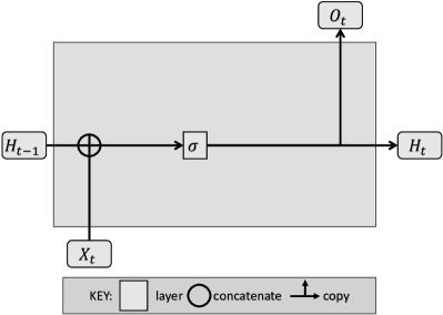
Figure 1: RNN architecture used for training; ($H_{t-1},H_{t}$) represent the hidden state, ($O_{t}$) represents the output state, and ($X_{t}$) represents the input information. The $\sigma$ represents the activation function that operates on the combined input and hidden state.

In Figure  1, the $X_{t}$ represents some input, $H_{t-1},H_{t}$ represents some hidden state (which is representative of memory), $O_{t}$ represents some output and $\sigma$ represents some activation function. The current input information combines with the previous hidden state, and the resulting combined state is then fed to an activation function to insert some non-linearity. This non-linearity produces the next hidden state, which can be further manipulated to create a desired output. The fundamental element is the hidden state which theoretically allows for consideration of any historical input and its effects on the current input. For a mathematical description of an RNN, we refer to Equation  1 and Equation  2.

$$H_{t}=\sigma(W_{HH}H_{t-1}+W_{XH}X_{t})$$ (1)

$$O_{t}=W_{HO}H_{t}$$ (2)

II-E Related Works

GROVER

The graph representation from the self-supervised message passing transformer (GROVER) model takes two forms, GROVER_base and GROVER_large [13]. For this paper, we only consider GROVER_large as it achieves the highest performance of the two. GROVER bases its design on popular large language models such as, BERT and GPT, where a large corpus of information pre-trains a model and fine-tuning is applied for the completion of downstream tasks [14, 15]. However, they stray from prior works that attempt training using the SMILES string format [16] and instead use graphs which they believe to be more expressive. Previous graph pre-training approaches use the available supervised labels to train their model [5], but GROVER believes a self-supervised approach would perform better, so they suggest using contextual property prediction and graph-level motif prediction. Contextual property prediction takes a given element (node) within a molecular graph and predicts the connected elements and the type of bond used for the connection. Graph-level motif prediction takes a given molecule and attempts to predict the recurrent sub-graphs, known as motifs, that may appear within the molecule. To build the model they designed a new architecture known as the GTransformer, which creates an attention-based understanding of molecular graphs. While this new architecture and self-supervised training approach offer appealing results the model uses 100M parameters, uses 250 Nvidia V100 GPUs, and takes four days for pre-training.

ChemRL-GEM

Geometry Enhanced Molecular representation learning method (GEM) for Chemical Representation Learning (ChemRL) (ChemRL-GEM) draws inspiration from previous works using a graph-based approach, especially GROVER [5, 13]. ChemRL-GEM uses a large corpus of information to pre-train a model and, like GROVER, believes the ambiguity of SMILES and lack of structural information make it hard to build a successful model using a string-based approach [17]. ChemRL-GEM believes the low performance of prior graph approaches is from neglecting the available molecular 3D information and improper pre-training tasks. ChemRL-GEM pre-training tasks are split into two types, geometry level, and graph level tasks. The geometry level tasks are again split into two types where bond length prediction, and bond angle prediction are local spatial structure predictions, and atomic distance matrices prediction is a global spatial prediction. The graph-level predictions are the Molecular ACCess System (MACCS) key prediction, and the extended-connectivity fingerprint (ECFP) prediction. To build the model they designed an architecture called GeoGNN which trains on the atom-bond graph and the bond-angle graph of molecules to build a 3D structure-based understanding of the molecular graphs. ChemRL-GEM achieves SOTA performance and is one of the first to attempt a large 3D graph model pre-trained network. However, their approach requires training with 20 million samples which would be time-consuming. They state pre-training a small subset of the data would take several hours using 1 Nvidia V100 GPU, and fine-tuning would require 1-2 days on the same GPU. As a rough estimate of the actual training process there was a follow-up work called LiteGEM which removed the 3D input of the model but still uses 74 million parameters and takes roughly ten days of training using 1 Nvidia V100 GPU [18].

Galactica

Galactica is inspired directly by previous large language models and their utilization of large data sets to pre-train models for downstream tasks [14, 15]. Differentiating themselves from GPT or BERT, they use a decoder-only setup from [19]. Unlike GROVER or ChemRL, Galactica focuses on general scientific knowledge and wishes to apply it to the entirety of the scientific domain [8]. The Galactica model takes several forms, but we focus our attention on the 120 billion parameter model as it offers the best performance. Galactica trains over 60 million individual scientific documents and 2 million SMILES strings. Galactica acknowledges while using SMILES they receive reduced performance gains as their model size increases, but they believe this could be overcome with more samples. Galactica offers a competitive performance to graph-based approaches while offering a simplified architecture design. Unfortunately, the model requires 120 billion parameters which are trained using 128 Nvidia A100 80GB nodes. Despite the massive model size, it is not SOTA for a single SMILES metric. This is likely due to their focus on building a general model, so they performed no fine-tuning to try to obtain SOTA results.

III Methods

Our goal is to achieve the highest possible performance by using a simple language model. Achieving this requires improvement in the data and the neural network.

III-A Data Pre-processing

The available SIDER data set uses SMILES for its molecular representation. After reviewing some of the molecule strings, not all are canonical. Including non-canonical SMILES is problematic as SMILES grammar is already complex; the molecules are converted to canonical form to reduce complexity. The next issue we address is caused by RNNs. One of the many advantages of RNN is the allowance of variable length inputs to account for a variable length of history. This is only true theoretically; in practice, memory is limited which is the focus of many newer works [20]. Despite this limitation, it has been recently shown that RNNs can handle input lengths of around 45-50 before the performance begins to degrade [21, 22]. Using this knowledge, we set a maximum length of 46 for the SMILES molecules. This keeps a minor majority of the molecules while allowing us to ensure the RNN is performing well. Figure  2 visualizes the molecule lengths within the SIDER data set.

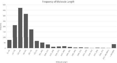
Figure 2: Histogram of molecule length in SIDER data set pre-canonization.

After limiting the SMILES molecular length, the SMILES are converted to SELFIES. The intention of converting SMILES to SELFIES is to reduce the grammar complexity and simplify the learning process of the RNN. SELFIES converts each element and structural component, such as rings or branches, into their label. These labels are then encoded into a numerical value based on their dictionary index.

III-B RNN Implementation

To achieve the best possible results from the vanilla RNN model, we insert an embedding layer before the RNN with a dimension the size of the label dictionary. This is to maintain as much information as possible. The input, hidden, and output dimensions of the RNN are also set to be the size of the label dictionary. We believe maintaining the dimensional space, and not reducing before output generation, will give the RNN the best chance of learning the context of the molecule. RNNs historically use the Tanh activation function, however, we use the LeakyReLU as it reduces saturation possibilities and typically results in higher performance [23, 24]. In addition to this, we also include a dropout layer on the output of the RNN which helps prevent overfitting and reduce the error rate of RNNs [25]. After processing the molecule through the RNN, the final state should have all important prior information encoded into it. This vector then passes through an additional LeakyReLU and dropout layer before being fed to a fully connected layer. The fully connected layer reduces the vector from the dictionary-sized dimension down to the number of classes present in the molecular property. A soft-max operation is then used to find the most likely class. Figure  3 contains an overview of the process described above.

Figure 3: Overview of the RNN process.

IV Results and Comparative Analysis

IV-A Results

Before training on SIDER, we perform an additional reduction to the data set by setting the lower bound of 31 molecules to the SMILES string allowing for the search space to remain sufficiently complex while reducing the overall run time. This reduces the data set to 400 molecules, which is then stratified split using 80% for training and 20% for testing [26]. The stratified split intends to maintain the known sample rate of a given side effect to model real-world testing. However, during training, we want to remove the bias of sampling to ensure our model is accurately learning the causes of a side effect. To reduce the bias in the training set, the minority samples within the training set are duplicated to have an even sample count between the side effect present and the side effect not present. After completing the replication of training samples, the SMILES strings are converted to SELFIES. Typical natural language processing (NLP) methods use a word, sub-word, or character tokenization to convert strings into numerical values, but we opt for a slightly different method which we explain by referring to equation  3. It shows the SELFIES representation of benzene where each molecule and structural element are between brackets. Using this representation we decide to tokenize based on each set of brackets that exist within the SELFIES converted data set. This results in a total of 47 unique values.

$$[C][=C][C][=C][C][=C][Ring1][=Branch1]$$ (3)

After tokenizing the SELFIES, the embedding dimension, input dimension of the RNN, and the hidden dimension of the RNN are set to a size of 47 to match the dimensional space of the tokens. To give the RNN model the best opportunity to make accurate classifications, we use a single RNN model to perform a single side effect classification prediction. Instead of predicting all 27 potential side effect classifications, we opt to predict 20 side effect classifications due to extreme imbalances present in the side effect data. The RNN architecture results in a model with 11.5K parameters training in under 2 minutes on an Nvidia GeForce RTX 3090. To compare our performance with other works that use SIDER we evaluate using the receiver operating characteristic curve (ROC) [1, 27]. The ROC scores for 20 side effect classification tasks are shown in Table I. While ROC is helpful for comparison, it is commonly misunderstood [28, 29] so we include a small sample of 3 training/testing accuracy and loss curves in Figure  4 as a simple spot check of model performance.

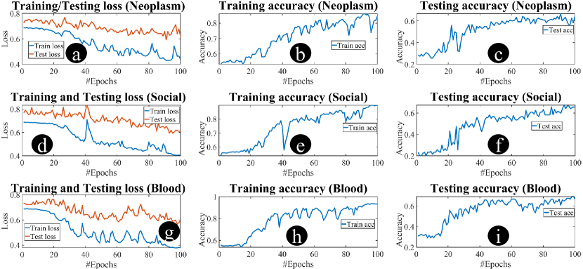
Figure 4: Results of three tasks: (a) loss curves, (b) training accuracy, (c) testing accuracy for neoplasms benign, malignant and unspecified (incl cysts and polyps) disorders, (d), (e), (f) for social circumstances disorders and (g), (h), (i) for blood and lymphatic system disorders.

Examining Figure  4, we note that training and testing loss is decreasing across all three side effect properties. There are spikes within each of the loss curves, but this is known to occur since the inception of RNNs [12]. The training loss for all three side effects appears to saturate faster than the testing. There can be some gap in performance in loss based on the difficulty of new samples, but the gap here is likely accentuated as an unfortunate side effect of the minority sample duplication process. The duplicate samples within the training set help the model learn what molecular components help detect a side effect, but during training, the repeated samples become easier to predict for the model. In the case of accuracy, both training and testing show an upward trending curve where improvement starts to attenuate between the 20th-40th epoch. This attenuation roughly matches the attenuation that occurs with the loss curves. Comparing training and testing accuracy there appears to be a roughly 20+% gap in performance at nearly every epoch, which we again attribute to the duplicate samples within the training set.

TABLE I: Table of ROC performance per molecular property prediction.

Property	ROC	Property	ROC
Blood	.57	Cardiac	.71
Congenital	.73	Ear	.69
Endocrine	.73	Eye	.73
Hepatobiliary	.63	immune	.68
Infections	.71	Injury	.77
Metabolism	.6	Musculoskeletal	.73
Neoplasms	.72	Psychiatric	.81
Renal	.6	Reproductive	.69
Respiratory	.5	Social	.5
Surgical	.5	Vascular	.82

IV-B Comparisons

To understand our model performance we compare it across multiple data sets to two top-performing GNN models, ChemRL-GEM [17] and GROVER_large [13], and a top-performing NLP model, Galactica [8]. Overall results are shown in Table II.

TABLE II: Table of ROC performance per molecular property prediction across data sets.

Test Proposed ChemRL-GEM [17] GROVER_large [13] Galactica [8] SIDER .671 .672 .658 .632 BBBP .73 .724 .940 .661 Clintox .75 .901 .944 .826 BACE .80 .856 .894 .617

Beginning with the SIDER test, the results in Table  II show our approach achieves .01% less than the SOTA model. While there are no direct statistics available for ChemRL-GEM, we use roughly 99.7% fewer parameters than its follow-up work, LiteGEM [17, 18]. For the BBBP test, we outperform ChemRL-GEM and Galactica but perform worse than GROVER_large. While it may be possible that GROVER achieves these results due to their usage of graph representation, it more likely stems from having 100M parameters, over 8,000x more parameters than our model [13]. For the Clintox test, our performance was unfortunately the lowest of all the models. Re-examining the Galactica work, we can outperform their 1.3B parameter model and are competitive with their 6.7B parameter model, meaning we can compete with an NLP model that has 80,000x more parameters [8]. Using BACE for evaluation, our model achieves the third highest score, a competitive performance coming in at only 9.4% less than the highest score received.

V Discussion & Conclusion

While large data models may offer slightly higher performance, we have shown that small models (specifically RNNs) are still viable candidates for molecular property prediction. Smaller models are cheaper, more practical, and more accessible solutions as they don’t require high-performance machines and billions of dollars to deploy. While there is a gap between the performance of the RNN model to the larger models, we believe it can be closed by continuing to focus on building more descriptive languages such as SELFIES [11].

References

- [1] K. Yang, K. Swanson, W. Jin, C. Coley, P. Eiden, H. Gao, A. Guzman-Perez, T. Hopper, B. Kelley, M. Mathea et al., “Analyzing learned molecular representations for property prediction,” Journal of chemical information and modeling, vol. 59, no. 8, pp. 3370–3388, 2019.
- [2] O. Wieder, S. Kohlbacher, M. Kuenemann, A. Garon, P. Ducrot, T. Seidel, and T. Langer, “A compact review of molecular property prediction with graph neural networks,” Drug Discovery Today: Technologies, vol. 37, pp. 1–12, 2020.
- [3] T. Lengauer, C. Lemmen, M. Rarey, and M. Zimmermann, “Novel technologies for virtual screening,” Drug discovery today, vol. 9, no. 1, pp. 27–34, 2004.
- [4] C. Merkwirth and T. Lengauer, “Automatic generation of complementary descriptors with molecular graph networks,” Journal of chemical information and modeling, vol. 45, no. 5, pp. 1159–1168, 2005.
- [5] W. Hu, B. Liu, J. Gomes, M. Zitnik, P. Liang, V. Pande, and J. Leskovec, “Strategies for pre-training graph neural networks,” arXiv preprint arXiv:1905.12265, 2019.
- [6] Z. Wu, S. Pan, F. Chen, G. Long, C. Zhang, and S. Y. Philip, “A comprehensive survey on graph neural networks,” IEEE transactions on neural networks and learning systems, vol. 32, no. 1, pp. 4–24, 2020.
- [7] A. Mayr, G. Klambauer, T. Unterthiner, M. Steijaert, J. K. Wegner, H. Ceulemans, D.-A. Clevert, and S. Hochreiter, “Large-scale comparison of machine learning methods for drug target prediction on chembl,” Chemical science, vol. 9, no. 24, pp. 5441–5451, 2018.
- [8] R. Taylor, M. Kardas, G. Cucurull, T. Scialom, A. Hartshorn, E. Saravia, A. Poulton, V. Kerkez, and R. Stojnic, “Galactica: A large language model for science,” arXiv preprint arXiv:2211.09085, 2022.
- [9] M. Kuhn, I. Letunic, L. J. Jensen, and P. Bork, “The sider database of drugs and side effects,” Nucleic acids research, vol. 44, no. D1, pp. D1075–D1079, 2016.
- [10] D. Weininger, “Smiles, a chemical language and information system. 1. introduction to methodology and encoding rules,” Journal of chemical information and computer sciences, vol. 28, no. 1, pp. 31–36, 1988.
- [11] M. Krenn, F. Häse, A. Nigam, P. Friederich, and A. Aspuru-Guzik, “Self-referencing embedded strings (selfies): A 100% robust molecular string representation,” Machine Learning: Science and Technology, vol. 1, no. 4, p. 045024, 2020.
- [12] J. L. Elman, “Finding structure in time,” Cognitive science, vol. 14, no. 2, pp. 179–211, 1990.
- [13] Y. Rong, Y. Bian, T. Xu, W. Xie, Y. Wei, W. Huang, and J. Huang, “Self-supervised graph transformer on large-scale molecular data,” Advances in Neural Information Processing Systems, vol. 33, pp. 12 559–12 571, 2020.
- [14] J. Devlin, M.-W. Chang, K. Lee, and K. Toutanova, “Bert: Pre-training of deep bidirectional transformers for language understanding,” arXiv preprint arXiv:1810.04805, 2018.
- [15] A. Radford, K. Narasimhan, T. Salimans, I. Sutskever et al., “Improving language understanding by generative pre-training,” 2018.
- [16] S. Wang, Y. Guo, Y. Wang, H. Sun, and J. Huang, “Smiles-bert: large scale unsupervised pre-training for molecular property prediction,” in Proceedings of the 10th ACM international conference on bioinformatics, computational biology and health informatics, 2019, pp. 429–436.
- [17] X. Fang, L. Liu, J. Lei, D. He, S. Zhang, J. Zhou, F. Wang, H. Wu, and H. Wang, “Chemrl-gem: Geometry enhanced molecular representation learning for property prediction,” arXiv preprint arXiv:2106.06130, 2021.
- [18] S. Zhang, L. Liu, S. Gao, D. He, X. Fang, W. Li, Z. Huang, W. Su, and W. Wang, “Litegem: Lite geometry enhanced molecular representation learning for quantum property prediction,” arXiv preprint arXiv:2106.14494, 2021.
- [19] A. Vaswani, N. Shazeer, N. Parmar, J. Uszkoreit, L. Jones, A. N. Gomez, Ł. Kaiser, and I. Polosukhin, “Attention is all you need,” Advances in neural information processing systems, vol. 30, 2017.
- [20] S. Hochreiter and J. Schmidhuber, “Long short-term memory,” Neural computation, vol. 9, no. 8, pp. 1735–1780, 1997.
- [21] X. Yao, Q. Cheng, and G.-Q. Zhang, “A novel independent rnn approach to classification of seizures against non-seizures,” arXiv preprint arXiv:1903.09326, 2019.
- [22] W. Yin, K. Kann, M. Yu, and H. Schütze, “Comparative study of cnn and rnn for natural language processing,” arXiv preprint arXiv:1702.01923, 2017.
- [23] A. L. Maas, A. Y. Hannun, A. Y. Ng et al., “Rectifier nonlinearities improve neural network acoustic models,” in Proc. icml, vol. 30, no. 1. Atlanta, Georgia, USA, 2013, p. 3.
- [24] B. Xu, N. Wang, T. Chen, and M. Li, “Empirical evaluation of rectified activations in convolutional network,” arXiv preprint arXiv:1505.00853, 2015.
- [25] Y. Gal and Z. Ghahramani, “A theoretically grounded application of dropout in recurrent neural networks,” Advances in neural information processing systems, vol. 29, 2016.
- [26] S. Thompson, Sampling, ser. CourseSmart. Wiley, 2012. [Online]. Available: https://books.google.com/books?id=-sFtXLIdDiIC
- [27] G. Zhou, Z. Gao, Q. Ding, H. Zheng, H. Xu, Z. Wei, L. Zhang, and G. Ke, “Uni-mol: A universal 3d molecular representation learning framework,” 2023.
- [28] J. A. Hanley and B. J. McNeil, “The meaning and use of the area under a receiver operating characteristic (roc) curve.” Radiology, vol. 143, no. 1, pp. 29–36, 1982, pMID: 7063747. [Online]. Available: https://doi.org/10.1148/radiology.143.1.7063747
- [29] T. Saito and M. Rehmsmeier, “The precision-recall plot is more informative than the roc plot when evaluating binary classifiers on imbalanced datasets,” PloS one, vol. 10, no. 3, p. e0118432, 2015.