CBAGAN-RRT: Convolutional Block Attention Generative Adversarial Network for Sampling-Based Path Planning

Abstract

Sampling-based path planning algorithms play an important role in autonomous robotics. However, a common problem among the RRT-based algorithms is that the initial path generated is not optimal and the convergence is too slow to be used in real-world applications. In this paper, we propose a novel image-based learning algorithm (CBAGAN-RRT) using a Convolutional Block Attention Generative Adversarial Network with a combination of spatial and channel attention and a novel loss function to design the heuristics, find a better optimal path, and improve the convergence of the algorithm both concerning time and speed. The probability distribution of the paths generated from our GAN model is used to guide the sampling process for the RRT algorithm. We train and test our network on the dataset generated by [55] and demonstrate that our algorithm outperforms the previous state-of-the-art algorithms using both the image quality generation metrics like IOU Score, Dice Score, FID score, and path planning metrics like time cost and the number of nodes. We conduct detailed experiments and ablation studies to illustrate the feasibility of our study and show that our model performs well not only on the training dataset but also on the unseen test dataset. The advantage of our approach is that we can avoid the complicated preprocessing in the state space, our model can be generalized to complicated environments like those containing turns and narrow passages without loss of accuracy, and our model can be easily integrated with other sampling-based path planning algorithms.

1 Introduction

Path planning is one of the fundamental topics in robotics which aims to find a collision-free path around obstacles in the environment. Various approaches have been proposed over the years like grid-based ones using Dijkstra’s and A* which suffer from the high time and memory cost as the dimensionality of the search space increases. Sampling-based path planning algorithm solves the aforementioned problem by drawing samples from the state space, constructing a random graph, and searching for a feasible path using the Probabilistic Roadmap (PRM) or the Rapidly Random Exploring Tree (RRT) thus offering better scalability to higher dimensional problems. A random graph is constructed in PRM after the sampling process and hence works better for multi-query problems while the random tree is constructed randomly and incrementally from the start to the goal node thus making it better for single-query problems. The best part about the RRT or the PRM-based algorithms is that they guarantee that a solution is found if it exists because of the probabilistic completeness property. However, sampling-based path planning algorithms’ convergence speed is slow and the initial paths generated are not optimal because they sample uniformly in the state space and have many time-consuming and repeated functions like collision checking and the tree rewiring operation in the case of the RRT* algorithm. The path quality generated is proven to be not optimal and these algorithms are too slow in challenging environments like those having many turns or narrow passages. In this work, we propose a novel GAN-based neural network that can quickly predict the probability distribution of feasible paths on a map before being fed to the sampling-based path planning algorithm thus speeding up the convergence both in terms of the time and the speed.

2 Related Work

Sampling-based path planning algorithms [18]have been highly successful in various robotics problems from autonomous driving to drones to warehouse robots. The first sampling-based path planning algorithm was the original RRT algorithm by [20] which solved several challenges faced by the grid-based algorithms like faster convergence and better initial solution. It was considered the perfect sweet spot between probabilistic road maps and grid-based path planning algorithms getting the best of both worlds as shown in [19] and [22].

[14] showed that the RRT* algorithm possesses asymptotically optimal property and the quality of the path generated was much better than the RRT algorithm using a novel rewiring operation and a novel nearest neighbor search operation. However, the algorithm was much slower than the RRT algorithm and it took a long time to converge and the paths obtained were not always correct. The RRT* algorithm works under holonomic constraints, offline planning mode, point kinematic model, uniform sampling strategy, and Euclidean term as the distance metric.

[15] proposed Anytime RRT* which was able to generate better trajectories using a branch and bound adaptation technique and committed trajectory technique and was able to generate better optimal paths while also speeding up the convergence thus demanding lesser computational resources. However, the paths generated were still not optimal in a lot of cases and the algorithm forced node removal while building the tree. Anytime RRT* algorithm works under non-holonomic constraints, online planning mode, Dublin car kinematic model, uniform sampling strategy, and a Euclidean plus a velocity term as the distance metric.

[33] proposed RRT* Smart which improved the efficiency and accelerated the rate of the convergence of the algorithm using a novel path optimization technique and intelligent sampling. However, this method had its drawbacks like manually defining the heuristics upon which the algorithm depended and the fact that there was a trade-off between exploration space and the convergence rate. The RRT* Smart algorithm works under holonomic constraints, offline planning mode, point kinematic model, intelligent sampling strategy, and Euclidean term as the distance metric.

Machine learning-based approaches have been applied and have had their share of success by either improving the heuristics to speed up the convergence of the algorithm or avoiding getting stuck in the local minimum. Deep learning powered by deep neural networks has ushered a new era in this domain and has been quite successful in solving various problems in sampling-based path planning [43], [44], [30], [1], [2], [52], [25], [3].

Recent years have also seen an advent of generative models like the Generative Adversarial Network like Pix2pix [11] and Variational Autoencoder to generate the promising region using paired labeled training data and have shown to outperform all previous numerical and algorithmic-based approaches while reducing the time taken, number of nodes, and the length of the initial path to convergence [55], [27], and [29]. Attention mechanism [42] has resulted in a breakthrough and has been a driving force behind various state-of-the-art architectures across modalities like computer vision and natural language processing [53], [45], [48], [5], and [5] and offers great potential in the image based path planning landscape.

3 Method

3.1 Path Planning Problem

Assuming the state space of the planning problem is represented by X and $X_{f}ree$ is the collision-free subspace of the state X. Then $X_{o}bs=X-X_{f}ree$ would denote the obstacle space in the map. Let’s assume the start and the goal state be represented by $x_{s}$ and $x_{g}$ and any 2 random points by $x_{1}$ and $x_{2}$ in the map. Let’s also denote the ball center of radius r at x by $B(x,r)$. The Euclidean distance between the 2 can be denoted by $x_{1}-x_{2}$. Assuming $\sigma$ denotes a feasible path and for the sequence of states we have $\sigma(0)$ = $x_{s}$, $\sigma(t)$ = $B(x_{g},r_{g}$ where $\sigma(t)\subset X_{f}ree$. Hence the cost of the optimal path can be represented by $c(\sigma)=\Sigma_{t=1}^{t}\sigma(t)-\sigma(t-1)$. The path length can be obtained by minimizing the cost function. The following definition is used in the RRT algorithm:

- V: Set of vertices in the sampling tree. - E: Set of edges between the vertices in the sampling tree. - Sample free: Procedure of sampling a random node from the state space. - Nearest(V, x): Finding the nearest node from the vertex V to point X using Euclidean distance as the metric. - Steer($x_{1}$, $x_{2}$): Steer from $x_{1}$ to $x_{2}$ along the path $\delta(t)$. - $Obs_{free}\delta(t)$: Find if a collision-free and feasible path exists in the map or not.

3.2 Dataset

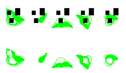
We used the dataset generated by [55] to validate our results. The dataset was generated by randomly placing different obstacles on the map and randomly sampling the start and goal nodes which are denoted by red and blue dots on the map respectively. The RRT algorithm was run to generate the feasible path which is shown in green color or the ground truth. The dimensions of all the images are (3x256x256) where the height and the width of the images are 256 and the number of channels is 3. We use 8000 images for training and 2000 images for testing respectively using the dataset by [55].

3.3 Data Augmentation

The parameters used in the data augmentation like height shift of the map, width shift of the map, shift step of the map, rotation probability of the map, and the number of maps generated of the map are shown below:

Table 1: Data Augmentation Parameters

Parameter	Value
Height shift of map	2
Width shift of map	2
Shift step of map	1
Rotation probability of map	0.5
Number of maps to be generated	10

The following data augmentation methods were used to increase the quality and quantity of the dataset:

1. Rescaling: We rescale the pixel values by rescaling factor 1/255.

2. Rotation: Random rotations with the setup degree range between [0, 360] was used.

3. Height and Width Shift: Shifting the input to the left or right and up or down was performed.

4. Shearing Intensity: It refers to the shear angle (unit in degrees) in a counter-clockwise direction.

5. Brightness: It uses a brightness shift value from the setup range.

A few sample ground truth images from the dataset generated by [55] showing the promising region in the environment map are illustrated below which goes into the training:

Figure 1: The first row shows images from the dataset with the white region as the free space, the black region as the obstacle space, the start node in color red, the goal node in color blue, and the green area as the promising region superimposed on the map. The second row shows only the promising region on the map. The promising region or the region of interest here is the ground truth labels which go into the training along with the images depicted in the first row.

3.4 Network Architecture

The fundamental goal in this image-based heuristic generation for the environment is to map an RGB image $X\in R^{H\times W\times 3}$ to a semantic map $Y\in R^{H\times W\times C}$ with the same spatial resolution $H\times W$, where $C$ is the number of classes of objects present in image which is 2, in this case, being the free space and the obstacle space respectively. The input image $X$ is converted to a set of feature maps ${F_{l}}$ where l=1,…,3 from each network stage, where $F_{l}\in R^{H_{l}×W_{l}×C_{l}}$ is a $C_{l}$-dimensional feature map. The input image is first passed through a block comprising convolutional, batch normalization, and ReLU activation functions. We express a convolution layer $W^{n}(x)$ as follows:

$$\mathrm{W}^{n}(x)=\mathbf{W}^{n\times n}\odot x+\mathbf{b}$$ (1)

where $\odot$ represents the convolution operator, $W^{n\times n}$ represents the $n\times n$ convolutional kernel, $x$ represents the input data and $b$ represents the bias vector.

3.4.1 Spatial Attention Module

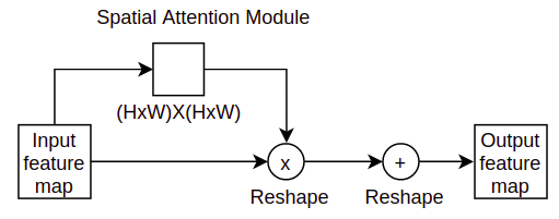
The spatial attention module is used for capturing the spatial dependencies of the feature maps. The spatial attention (SA) module in our network is defined below:

$$f_{{SA}}(x)=f_{sigmoid}\left({W}_{2}\left(f_{{ReLU}}\left({W}_{1}(x)\right)\right)\right)$$ (2)

where $W_{1}$ and $W_{2}$ denotes the first and second $1\times 1$ convolution layer respectively, $x$ denotes the input data, $f_{Sigmoid}$ denotes the sigmoid function, $f_{ReLU}$ denotes the ReLu activation function. The spatial attention module used in this work is shown in the figure below:

Figure 2: Details of our spatial attention module

.

3.4.2 Channel Attention Module

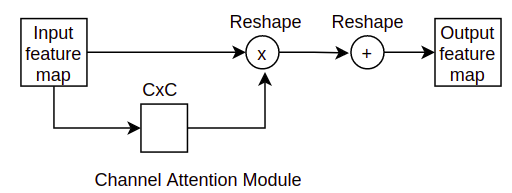
The channel attention module is used for extracting high-level multi-scale semantic information. The channel attention (CA) module in our network is defined below:

$$f_{{CA}}(x)=f_{sigmoid}({W}_{2}(f_{{ReLU}}({W}_{1}f_{{AvgPool}}^{1}(x))))$$ (3)

where $W_{1}$ and $W_{2}$ denotes the first and second $1\times 1$ convolution layer, $x$ denotes the input data. $f^{1}_{AvgPool}$ denotes the global average pooling function, $f_{Sigmoid}$ denotes the Sigmoid function, $f_{ReLU}$ denotes ReLU activation function. The channel attention module used in this work is shown in the figure below:

Figure 3: Details of our channel attention module

.

3.4.3 Convolutional Block Attention Generative Adversarial Network

GANs are a family of unsupervised generative models which learns to generate samples from a given distribution [9]. Given a noise distribution, Generator $G$ tries to generate samples while the Discriminator $D$ tries to tell whether the generated samples are from the correct distribution or not. Both the generator and discriminator are trying to fool each other, thus playing a zero-sum game. In other words, both are in a state of Nash Equilibrium. Let $G$ represent the generator, $D$ the discriminator, loss function used for training GAN can be written as shown in Equation 1:

$$\mathcal{F}(\mathcal{D},\mathcal{G})=\mathbb{E}_{\mathbf{x}\sim p_{\mathbf{x}}}[-\log\mathcal{D}(\mathbf{x})]+\\ \mathbb{E}_{\mathbf{z}\sim p_{\mathbf{z}}}[-\log(1-\mathcal{D}(\mathcal{G}(\mathbf{z})))]$$ (4)

where $z$ is latent vector, $x$ is data sample, $p_{z}$ is probability distribution over latent space and $p_{x}$ is the probability distribution over data samples. The zero-sum condition is defined in Equation 2:

$$\min_{G}\max_{D}\mathcal{F}(\mathcal{D},\mathcal{G})$$ (5)

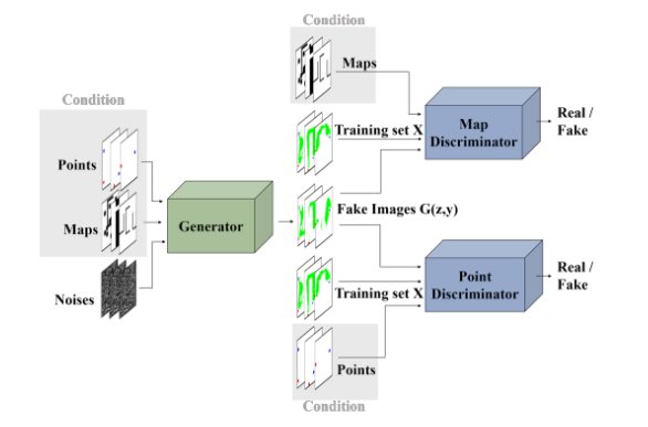
The Convolutional layer has a kernel size of 4, a stride of 2, a padding of 1, and uses batch normalization and LeakyReLU as the activation function. The Transposed Convolutional layer uses a kernel size of 4, a stride of 2, and padding of 1, and uses instance normalization and LeakyReLU as the activation function. The number of input and output channels in the Residual Block is 128. The kernel size is 4, the stride is 2, the padding is 1, and uses instance normalization and ReLU as the activation function. The Convolutional Block Attention Module shown has a reduction in channel attention value of 16, number of channels in the input layer of channel attention as 512, kernel size in spatial attention of 7, uses ReLU as the activation function, and Kaiming type as the weight initialization. The parameters for the Generator in our GAN are: the number of map input channels is 3, the number of point input channels is 3, the number of noise channels is 1, the number of hidden channels is 64, and the number of output (ROI) channels is 3. The parameters used in the Map Discriminator of our GAN are the number of Map channels as 3, the number of ROI channels as 3, the number of hidden channels as 64, and the number of output (ROI) channels as 1. The parameters used in the Point Discriminator of our GAN are the number of Point channels as 3, the number of ROI channels as 3, the number of hidden channels as 64, and the number of output (ROI) channels as 1. The overall structure of our GAN network is shown in the figure below:

Figure 4: Details of the GAN network architecture

.

3.5 Loss Functions

A combination of binary cross entropy and dice losses has been used to train the network. The first part binary cross-entropy is a commonly used loss function for classification problems as shown by [8]. Every pixel in the image needs to be classified and hence loss function can be written as shown in the equation below:

$$\mathcal{L}_{CE}=-\sum_{i,j}y_{i,j}\log\widehat{y}_{i,j}+\left(1-y_{i,j}\right)\log\left(1-\widehat{y}_{i,j}\right)$$ (6)

The first of them is a binary cross-entropy loss in the x-direction as shown below:

$$L_{bce}^{x}\left(\mathcal{P}^{x},\hat{\mathcal{P}}^{x}\right)=\sum_{i=1}^{H}\sum_{j=1}^{W}\mathcal{P}_{i,j}^{x}\log\left(\hat{\mathcal{P}}_{i,j}^{x}\right)+\\ \left(1-\mathcal{P}_{i,j}^{x}\right)\log\left(1-\hat{\mathcal{P}}_{i,j}^{x}\right)$$ (7)

A similar binary cross-entropy loss term is also used in the y-direction. The total binary cross entropy loss term can be obtained by summing up the two individual terms as shown below:

$$L_{bce}^{xy}(\mathcal{P},\hat{\mathcal{P}})=L_{bce}^{x}\left(\mathcal{P}^{x},\hat{\mathcal{P}}^{x}\right)+L_{bce}^{y}\left(\mathcal{P}^{y},\hat{\mathcal{P}}^{y}\right)$$ (8)

The problem with binary cross entropy loss is that it doesn’t take into account the class imbalance as the background is the dominant class. This is one of the fundamental challenges in image segmentation problems. Dice Loss is robust to the aforementioned problem which is based on Dice Similarity Coefficient as defined using the equation below:

$$L_{\text{dice }}^{xy}(\mathcal{P},\hat{\mathcal{P}})=1-\frac{2\left|\mathcal{P}^{x}\cap\hat{\mathcal{P}}^{x}\right|+2\left|\mathcal{P}^{y}\cap\hat{\mathcal{P}}^{y}\right|}{\left|\mathcal{P}^{x2}\right|+\left|\hat{\mathcal{P}}^{x2}\right|+\left|\mathcal{P}^{y2}\right|+\left|\hat{\mathcal{P}}^{y2}\right|}$$ (9)

Hence, the total loss can be obtained which is a summation of the binary cross-entropy loss and dice loss which is used for training the model is shown below:

$$L(\mathcal{P},\hat{\mathcal{P}})=L_{\text{bce }}^{xy}(\mathcal{P},\hat{\mathcal{P}})+L_{\text{dice }}^{xy}(\mathcal{P},\hat{\mathcal{P}})$$ (10)

The loss function used for training the map discriminator can be represented as shown below:

$$\mathcal{L}_{D_{\text{map }}}=L(\mathcal{P},\hat{\mathcal{P}})+ \mathbb{E}\left[\log D_{\text{map }}(s,m)\right]+$$ (11)

$$\left.\mathbb{E}_{[}\log\left(1-D_{\text{map }}(G(z,m,p),m)\right)\right]$$

The loss function used for training the point discriminator can be represented as shown below:

$$\mathcal{L}_{D_{\text{point }}}=L(\mathcal{P},\hat{\mathcal{P}})+ \mathbb{E}\left[\log D_{\text{point }}(s,p)\right]+$$ (12)

$$\left.\mathbb{E}_{[}\log\left(1-D_{\text{point }}(G(z,m,p),p)\right)\right]$$

The mean square pixel-wise loss function is defined using the below equation:

$$\mathcal{L}_{mse}(X,Y)=\ell_{mse}(G(X),Y)=\|G(X)-Y\|^{2}$$ (13)

Hence, the loss function used for training the generator can be represented as shown below:

$$\mathcal{L}_{G}= \alpha_{1}\mathbb{E}\left[\log D_{\text{map }}(G(z,m,p),m)\right]+$$ (14)

$$\alpha_{2}\mathbb{E}\left[\log D_{\text{point }}(G(z,m,p),p)\right]+\mathcal{L}_{mse}(X,Y)$$

3.6 Path Planning Algorithm

The RRT algorithm is used for single-query applications and is suitable for dealing with high-dimensional problems. The algorithm incrementally builds a tree of feasible paths rooted at a start node by randomly expanding nodes in a collision-free space. Initially, there is an empty vertex set V, edge set E, and an initial state. At every iteration, a node is randomly sampled and the nearest node of the existing vertex sex V is connected to the new sampling node. The vertex set and the edge set get added if the connection works. The process keeps on repeating until a new sampling node in the goal region is contained in the expanding tree. Space-filling trees are constructed to search a path connecting start and goal nodes while incrementally drawing random samples from the free space. We generate the promising region using GAN to generate the heuristics which denotes that a feasible path exists with a high probability. We use RRT as the sampling-based path-planning algorithm. We use our pre-trained GAN model to guide the sampling process of the RRT algorithm. The algorithm attempts to find the nearest vertex to the new sample and connect them and the new vertex is added to the vertex set V and the edge is added to the edge set E if no obstacles are present in the connection. Finally, the algorithm returns a new vertex set V and edge set E. The Heuristic RRT algorithm used in this work is shown below:

Algorithm 1: RRT Algorithm

⬇

RRT(Map, start, goal)

qs = [start]

qs_parent = [0]

while True{

q_rand = random_vertex_generated()

n_idx,q_near = nearest_vertex_check(q_rand)

q_new = new_point_generate(q_near,

q_rand,

n_idx)

if connection_check(q_new){

break

}

}

3.7 Training Details

We train the model on Nvidia T4 GPU in Pytorch using mini-batch Stochastic Gradient Descent (SGD) as the optimizer. The momentum and weight decay of the optimizer is set to 0.9 and 0.0001 respectively. We use exponential decay as the learning rate scheduler. We train the model for 50 epochs and 8 as the batch size. The input maps and the ground truth feasible region map are combined and sent to training. There are 200 different types of environment maps present in the dataset.

3.8 Evaluation Metrics

We use the time cost which represents the time taken for the algorithm to find a solution and the number of nodes which denotes the number of nodes explored on the way to solve as the path planning metrics to evaluate the quality of our algorithm from the path planning perspective. We use Dice Score (Dice) also known as F1-score and Intersection over union (IoU) as image quality metrics to evaluate the performance of our network. Here True positive (TR), false negative (FN), and false positive (FP) number of pixels calculated can be calculated separately for each image and averaged over the test set. The corresponding equations for both these metrics are shown using the equation below respectively.

$$\mathrm{Dice}=\frac{2TP}{2TP+FN+FP}$$ (15)

$$\mathrm{IoU}=\frac{TP}{TP+FN+FP}$$ (16)

We also use Fréchet Inception Distance (FID) to evaluate the quality of generated promising regions. A lower FID is preferred for better-performing generative models. Let $D$ represent the CNN used to extract features, ($m_{r}$, $\sigma_{r}$) be the mean and covariance of features extracted from real samples, and ($m_{f}$, $\sigma_{f}$) be mean and covariance of features extracted from fake samples with $D$, then the Frechet Inception distance is defined using the below equation:

$$d^{2}\left(\left(m_{r},\Sigma_{r}\right),\left(m_{f},\Sigma_{f}\right)\right)=\left\|m_{r}-m_{f}\right\|_{2}^{2}+\\ \operatorname{Tr}\left(\Sigma_{r}+\Sigma_{f}-2\left(\Sigma_{r}\Sigma_{f}\right)^{1/2}\right)$$ (17)

3.9 Experimental Details

The hyperparameters used in training our model like the batch size, number of epochs, generator learning rate, map discriminator learning rate, point discriminator learning rate, and the optimizer type with its parameters are shown below:

Table 2: Hyperparameters

Parameter	Value
Batch Size	8
Epochs	20
Generator Learning Rate	0.0001
Map Discriminator Learning Rate	0.00005
Point Discriminator Learning Rate	0.00005
Optimizer	Adam

In addition to the above hyperparameters, the exponential learning rate scheduler and ReduceLROnPlateau were used. In gradient descent, the value of momentum was taken as 0.9, $\gamma$ value of 0.1, and weight decay of 0.0005. The hyperparameter values for the Adam optimizer are ($\beta_{1}$ = 0.5, $\beta_{2}$ = 0.999. The parameters used in the various loss functions like Dice loss, IOU loss, Pixel Wise MSE loss, Pixel Wise L1 loss, generator loss, self-attention generator loss, and adaptive self-attention generator loss which goes into training are shown below:

Table 3: Loss Function Parameters

Parameter	Value
$\alpha$ in Dice loss	10
The smooth parameter in Dice loss	1
$\alpha$ in IOU loss	10
The smooth parameter in IOU loss	1
$\alpha$ in Pixel Wise MSE loss	20
$\alpha$ in Generator loss	100
$\alpha$ in CBAM Generator loss	1
$\beta$ in CBAM Generator loss	1
$\alpha$ in Adaptive CBAM Generator loss	3

The parameters used in the RRT path planning algorithm are shown below:

Table 4: RRT Algorithm Parameters

Parameter	Value
Step Length	0.2
Maximum Iterations	5000
Resolution of path	1

4 Results

Our GAN model outperforms the GAN model by [55] using IOU, Dice, and FID as the image quality evaluation metrics. Moreover, our model has a lesser number of parameters and thus takes lesser time for both training and inference which makes it a better choice for use as a heuristic for a sampling-based path planning algorithm as shown in Table 5:

Table 5: Comparison of our results vs state of the art networks using IOU, Dice, FID, and the number of parameters as the evaluation metrics.

Metrics	IOU	Dice	FID	No. of Parameters
SAGAN [55]	88.45	93.50	66.47	1.24 Million
Our Network	89.22	94.16	62.04	0.88 Million

The qualitative comparison of our results using CBAGAN-RRT versus the state-of-the-art network architecture SAGAN-RRT in terms of the promising region generated is shown in Figure 5:

Figure 5: Illustration of the comparison of results obtained. The first column shows the obstacle map with the white region as the free space and the black region as the obstacle space. The second column shows the promising region of the ground truth maps which goes into the training. The third column shows the promising region generated using the Self-Attention Generative Adversarial Network used in [55]. The fourth column shows the promising region generated using our Convolutional Block Attention Generative Adversarial Network. The red and the black nodes in all the maps denote the start and goal nodes respectively.

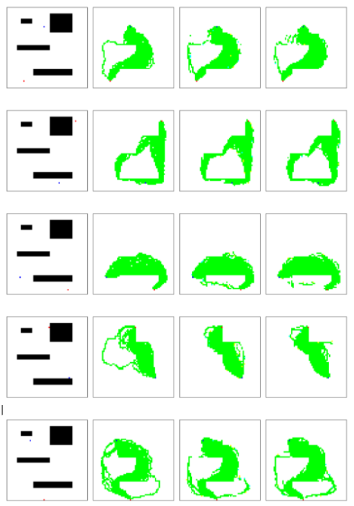
Our model outperforms the previous state-of-the-art network architecture using both the time cost and the number of nodes as the path planning evaluation metric. The comparison of using various algorithms like the original RRT algorithm, SAGAN-RRT, and our CBAGAN-RRT network as the heuristic for the path planning algorithm using time cost and the number of nodes is shown in Table 6:

Table 6: Comparison of our results versus RRT and SAGAN-RRT on 3 different maps using time cost and the number of nodes as the path planning evaluation metrics.

Map	Algorithm	Time Cost(s)	Number of Nodes
Map1	RRT	2.12	202
Map1	SAGAN [55]	1.37	157
Map1	Our Network	1.26	143
Map2	RRT	3.65	351
Map2	SAGAN [55]	2.40	246
Map2	Our Network	2.08	218
Map3	RRT	1.85	184
Map3	SAGAN [55]	1.28	129
Map3	Our Network	1.06	110

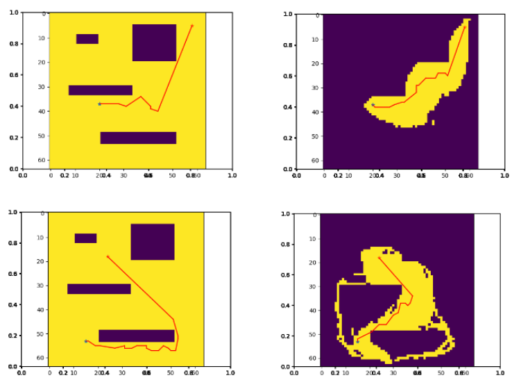
The qualitative comparison of our results using CBAGAN-RRT versus the original RRT in terms of the path generated is shown in Figure 6:

Figure 6: Illustration of our results using CBAGAN-RRT versus the original RRT in terms of the path generated. The left image depicts the path generated on the original obstacle map where the obstacles are shown in the dark color and the light color denotes the free space. The right image depicts the path generated using only the region of interest generated from our GAN model where the lighter color denotes the area inside the region of interest while the darker color denotes the region outside the region of interest. Only the region of interest is used for finding the feasible path and because the area is much smaller than that in the other image, we can improve the speed of convergence of the algorithm. The start and the goal nodes are shown in color blue and red respectively while the red line denotes the path taken.

4.1 Ablation Study

We conduct experiments using all the combinations of using spatial and channel attention modules and noticed that the best results using IOU, Dice, and FID as the image quality metrics and the time cost and number of nodes as the path planning metrics were achieved by using a combination of both spatial and channel attention modules in our network architecture as shown in Table 7:

Table 7: Comparison of our results with a combination of spatial and channel attention modules using IOU, Dice, and FID as the image quality evaluation metrics and time cost and the number of nodes as the path planning metrics.

Spatial Attention	Channel Attention	IOU	Dice	FID	Time Cost	No. of Nodes
$\checkmark$	$\checkmark$	85.22	95.86	65.47	1.08	127
$\checkmark$	$\times$	83.56	92.69	75.74	2.02	193
$\times$	$\checkmark$	84.73	94.06	66.49	1.75	166
$\times$	$\times$	83.08	92.10	82.53	2.56	235

We also conduct experiments using different attention modules and noticed that CBAM using a combination of spatial and channel attention modules led to the best results using IOU, Dice, and FID as the image quality metrics and the time cost and number of nodes as the path planning metrics as shown in Table 8:

Table 8: Comparison of our results with various attention modules like Convolutional Block Attention Module, Dual Attention Module, Efficient Channel Attention Module, Efficient Multi-Scale Attention Module, and Shuffle Attention Module using IOU, Dice, and FID as the image quality metrics and the time cost and number of nodes as the path planning metrics.

Attention Module	IOU	Dice	FID	Time Cost	No. of Nodes
CBAM [48]	85.22	95.86	65.47	1.08	127
DAModule [5]	84.54	94.29	68.45	1.23	146
ECAAttention [45]	84.81	94.05	72.41	1.34	150
ShuffleAttention [54]	85.06	95.42	70.56	1.16	133
TripletAttention [31]	83.60	92.87	77.15	1.40	164
SKAttention [24]	84.58	93.70	69.95	1.28	150
SpatialGroupEnhance [23]	83.82	94.99	72.63	1.42	142
SEAttention [10]	83.19	93.15	71.75	1.27	139
CoTAttention [26]	84.14	94.06	69.25	1.36	145

5 Conclusions and Future Work

In this paper, we proposed a novel image-based approach using convolutional block attention-based Generative Adversarial Network network CBAGAN-RRT to design the heuristics and find better optimal solutions and improve the convergence thus reducing the computational requirements for sampling-based path planning algorithms. We use the predicted probability distribution of paths generated from our model to guide the sampling process of the RRT algorithm. We demonstrate that our approach performs better than the state-of-the-art approach both in terms of the quality of feasible paths generated from an image perspective using IOU, Dice, and FID as the evaluation metrics as well as metrics like time cost and several nodes, from the path planning perspective. Our algorithm CBAGAN-RRT differs only in the sampling strategy from the RRT algorithm hence it can be easily integrated with other sampling-based path planning algorithms. A future idea could be to solve the problem by mapping it only as image segmentation and not image generation that is segmenting the feasible region using a state-of-the-art image segmentation algorithm and feeding that as heuristics for the path planning to improve the results. Another idea could be to integrate our GAN model with other sampling-based path-planning algorithms to study, test and validate the effectiveness of our approach.

References

- [1] Oktay Arslan and Panagiotis Tsiotras. Machine learning guided exploration for sampling-based motion planning algorithms. In 2015 IEEE/RSJ International Conference on Intelligent Robots and Systems (IROS), pages 2646–2652. IEEE, 2015.
- [2] Brendan Burns and Oliver Brock. Sampling-based motion planning using predictive models. In Proceedings of the 2005 IEEE international conference on robotics and automation, pages 3120–3125. IEEE, 2005.
- [3] Xuzhe Dang, Lukáš Chrpa, and Stefan Edelkamp. Deep rrt. In Proceedings of the International Symposium on Combinatorial Search, volume 15, pages 333–335, 2022.
- [4] Mohamed Elbanhawi and Milan Simic. Sampling-based robot motion planning: A review. Ieee access, 2:56–77, 2014.
- [5] Jun Fu, Jing Liu, Haijie Tian, Yong Li, Yongjun Bao, Zhiwei Fang, and Hanqing Lu. Dual attention network for scene segmentation. In Proceedings of the IEEE/CVF conference on computer vision and pattern recognition, pages 3146–3154, 2019.
- [6] Jonathan D Gammell, Siddhartha S Srinivasa, and Timothy D Barfoot. Informed rrt: Optimal sampling-based path planning focused via direct sampling of an admissible ellipsoidal heuristic. In 2014 IEEE/RSJ International Conference on Intelligent Robots and Systems, pages 2997–3004. IEEE, 2014.
- [7] Yi Gan, Bin Zhang, Chao Ke, Xiaofeng Zhu, Weiming He, and Tohru Ihara. Research on robot motion planning based on rrt algorithm with nonholonomic constraints. Neural Processing Letters, 53:3011–3029, 2021.
- [8] Ian Goodfellow, Yoshua Bengio, and Aaron Courville. Deep learning. MIT press, 2016.
- [9] Ian Goodfellow, Jean Pouget-Abadie, Mehdi Mirza, Bing Xu, David Warde-Farley, Sherjil Ozair, Aaron Courville, and Yoshua Bengio. Generative adversarial nets. In Advances in neural information processing systems, pages 2672–2680, 2014.
- [10] Jie Hu, Li Shen, and Gang Sun. Squeeze-and-excitation networks. In Proceedings of the IEEE conference on computer vision and pattern recognition, pages 7132–7141, 2018.
- [11] Phillip Isola, Jun-Yan Zhu, Tinghui Zhou, and Alexei A Efros. Image-to-image translation with conditional adversarial networks. In Proceedings of the IEEE conference on computer vision and pattern recognition, pages 1125–1134, 2017.
- [12] In-Bae Jeong, Seung-Jae Lee, and Jong-Hwan Kim. Rrt*-quick: A motion planning algorithm with faster convergence rate. In Robot Intelligence Technology and Applications 3: Results from the 3rd International Conference on Robot Intelligence Technology and Applications, pages 67–76. Springer, 2015.
- [13] In-Bae Jeong, Seung-Jae Lee, and Jong-Hwan Kim. Quick-rrt*: Triangular inequality-based implementation of rrt* with improved initial solution and convergence rate. Expert Systems with Applications, 123:82–90, 2019.
- [14] Sertac Karaman and Emilio Frazzoli. Sampling-based algorithms for optimal motion planning. The international journal of robotics research, 30(7):846–894, 2011.
- [15] Sertac Karaman, Matthew R Walter, Alejandro Perez, Emilio Frazzoli, and Seth Teller. Anytime motion planning using the rrt. In 2011 IEEE international conference on robotics and automation, pages 1478–1483. IEEE, 2011.
- [16] James J Kuffner and Steven M LaValle. Rrt-connect: An efficient approach to single-query path planning. In Proceedings 2000 ICRA. Millennium Conference. IEEE International Conference on Robotics and Automation. Symposia Proceedings (Cat. No. 00CH37065), volume 2, pages 995–1001. IEEE, 2000.
- [17] Yoshiaki Kuwata, Gaston A Fiore, Justin Teo, Emilio Frazzoli, and Jonathan P How. Motion planning for urban driving using rrt. In 2008 IEEE/RSJ International Conference on Intelligent Robots and Systems, pages 1681–1686. IEEE, 2008.
- [18] Steven M LaValle. Planning algorithms. Cambridge university press, 2006.
- [19] Steven M LaValle, Michael S Branicky, and Stephen R Lindemann. On the relationship between classical grid search and probabilistic roadmaps. The International Journal of Robotics Research, 23(7-8):673–692, 2004.
- [20] Steven M LaValle et al. Rapidly-exploring random trees: A new tool for path planning. 1998.
- [21] Steven M LaValle and James J Kuffner. Rapidly-exploring random trees: Progress and prospects: Steven m. lavalle, iowa state university, a james j. kuffner, jr., university of tokyo, tokyo, japan. Algorithmic and computational robotics, pages 303–307, 2001.
- [22] Steven M LaValle and James J Kuffner Jr. Randomized kinodynamic planning. The international journal of robotics research, 20(5):378–400, 2001.
- [23] Xiang Li, Xiaolin Hu, and Jian Yang. Spatial group-wise enhance: Improving semantic feature learning in convolutional networks. arXiv preprint arXiv:1905.09646, 2019.
- [24] Xiang Li, Wenhai Wang, Xiaolin Hu, and Jian Yang. Selective kernel networks. In Proceedings of the IEEE/CVF conference on computer vision and pattern recognition, pages 510–519, 2019.
- [25] Yang Li, Rongxin Cui, Zhijun Li, and Demin Xu. Neural network approximation based near-optimal motion planning with kinodynamic constraints using rrt. IEEE Transactions on Industrial Electronics, 65(11):8718–8729, 2018.
- [26] Yehao Li, Ting Yao, Yingwei Pan, and Tao Mei. Contextual transformer networks for visual recognition. IEEE Transactions on Pattern Analysis and Machine Intelligence, 2022.
- [27] Han Ma, Chenming Li, Jianbang Liu, Jiankun Wang, and Max Q-H Meng. Enhance connectivity of promising regions for sampling-based path planning. IEEE Transactions on Automation Science and Engineering, 2022.
- [28] Liang Ma, Jianru Xue, Kuniaki Kawabata, Jihua Zhu, Chao Ma, and Nanning Zheng. Efficient sampling-based motion planning for on-road autonomous driving. IEEE Transactions on Intelligent Transportation Systems, 16(4):1961–1976, 2015.
- [29] Nachuan Ma, Jiankun Wang, Jianbang Liu, and Max Q-H Meng. Conditional generative adversarial networks for optimal path planning. IEEE Transactions on Cognitive and Developmental Systems, 14(2):662–671, 2021.
- [30] Troy McMahon, Aravind Sivaramakrishnan, Edgar Granados, Kostas E Bekris, et al. A survey on the integration of machine learning with sampling-based motion planning. Foundations and Trends® in Robotics, 9(4):266–327, 2022.
- [31] Diganta Misra, Trikay Nalamada, Ajay Uppili Arasanipalai, and Qibin Hou. Rotate to attend: Convolutional triplet attention module. In Proceedings of the IEEE/CVF Winter Conference on Applications of Computer Vision, pages 3139–3148, 2021.
- [32] Kourosh Naderi, Joose Rajamäki, and Perttu Hämäläinen. Rt-rrt* a real-time path planning algorithm based on rrt. In Proceedings of the 8th ACM SIGGRAPH Conference on Motion in Games, pages 113–118, 2015.
- [33] Jauwairia Nasir, Fahad Islam, Usman Malik, Yasar Ayaz, Osman Hasan, Mushtaq Khan, and Mannan Saeed Muhammad. Rrt*-smart: A rapid convergence implementation of rrt. International Journal of Advanced Robotic Systems, 10(7):299, 2013.
- [34] Iram Noreen, Amna Khan, and Zulfiqar Habib. A comparison of rrt, rrt* and rrt*-smart path planning algorithms. International Journal of Computer Science and Network Security (IJCSNS), 16(10):20, 2016.
- [35] Iram Noreen, Amna Khan, and Zulfiqar Habib. Optimal path planning using rrt* based approaches: a survey and future directions. International Journal of Advanced Computer Science and Applications, 7(11), 2016.
- [36] Alejandro Perez, Robert Platt, George Konidaris, Leslie Kaelbling, and Tomas Lozano-Perez. Lqr-rrt*: Optimal sampling-based motion planning with automatically derived extension heuristics. In 2012 IEEE International Conference on Robotics and Automation, pages 2537–2542. IEEE, 2012.
- [37] Jie Qi, Hui Yang, and Haixin Sun. Mod-rrt*: A sampling-based algorithm for robot path planning in dynamic environment. IEEE Transactions on Industrial Electronics, 68(8):7244–7251, 2020.
- [38] Oren Salzman and Dan Halperin. Asymptotically near-optimal rrt for fast, high-quality motion planning. IEEE Transactions on Robotics, 32(3):473–483, 2016.
- [39] Marlin P Strub and Jonathan D Gammell. Adaptively informed trees (ait*) and effort informed trees (eit*): Asymmetric bidirectional sampling-based path planning. The International Journal of Robotics Research, 41(4):390–417, 2022.
- [40] Zaid Tahir, Ahmed H Qureshi, Yasar Ayaz, and Raheel Nawaz. Potentially guided bidirectionalized rrt* for fast optimal path planning in cluttered environments. Robotics and Autonomous Systems, 108:13–27, 2018.
- [41] Konstantinos I Tsianos, Ioan A Sucan, and Lydia E Kavraki. Sampling-based robot motion planning: Towards realistic applications. Computer Science Review, 1(1):2–11, 2007.
- [42] Ashish Vaswani, Noam Shazeer, Niki Parmar, Jakob Uszkoreit, Llion Jones, Aidan N Gomez, Łukasz Kaiser, and Illia Polosukhin. Attention is all you need. Advances in neural information processing systems, 30, 2017.
- [43] Jiankun Wang, Xiao Jia, Tianyi Zhang, Nachuan Ma, and Max Q-H Meng. Deep neural network enhanced sampling-based path planning in 3d space. IEEE Transactions on Automation Science and Engineering, 19(4):3434–3443, 2021.
- [44] Jiankun Wang, Tingguang Li, Baopu Li, and Max Q-H Meng. Gmr-rrt*: Sampling-based path planning using gaussian mixture regression. IEEE Transactions on Intelligent Vehicles, 7(3):690–700, 2022.
- [45] Qilong Wang, Banggu Wu, Pengfei Zhu, Peihua Li, Wangmeng Zuo, and Qinghua Hu. Eca-net: Efficient channel attention for deep convolutional neural networks. In Proceedings of the IEEE/CVF conference on computer vision and pattern recognition, pages 11534–11542, 2020.
- [46] Dustin J Webb and Jur Van Den Berg. Kinodynamic rrt*: Asymptotically optimal motion planning for robots with linear dynamics. In 2013 IEEE international conference on robotics and automation, pages 5054–5061. IEEE, 2013.
- [47] Kun Wei and Bingyin Ren. A method on dynamic path planning for robotic manipulator autonomous obstacle avoidance based on an improved rrt algorithm. Sensors, 18(2):571, 2018.
- [48] Sanghyun Woo, Jongchan Park, Joon-Young Lee, and In So Kweon. Cbam: Convolutional block attention module. In Proceedings of the European conference on computer vision (ECCV), pages 3–19, 2018.
- [49] Zhenping Wu, Zhijun Meng, Wenlong Zhao, and Zhe Wu. Fast-rrt: A rrt-based optimal path finding method. Applied Sciences, 11(24):11777, 2021.
- [50] Wang Xinyu, Li Xiaojuan, Guan Yong, Song Jiadong, and Wang Rui. Bidirectional potential guided rrt* for motion planning. IEEE Access, 7:95046–95057, 2019.
- [51] Chengke Xiong, Hexiong Zhou, Di Lu, Zheng Zeng, Lian Lian, and Caoyang Yu. Rapidly-exploring adaptive sampling tree*: a sample-based path-planning algorithm for unmanned marine vehicles information gathering in variable ocean environments. Sensors, 20(9):2515, 2020.
- [52] Chenning Yu and Sicun Gao. Reducing collision checking for sampling-based motion planning using graph neural networks. Advances in Neural Information Processing Systems, 34:4274–4289, 2021.
- [53] Han Zhang, Ian Goodfellow, Dimitris Metaxas, and Augustus Odena. Self-attention generative adversarial networks. In International conference on machine learning, pages 7354–7363. PMLR, 2019.
- [54] Qing-Long Zhang and Yu-Bin Yang. Sa-net: Shuffle attention for deep convolutional neural networks. In ICASSP 2021-2021 IEEE International Conference on Acoustics, Speech and Signal Processing (ICASSP), pages 2235–2239. IEEE, 2021.
- [55] Tianyi Zhang, Jiankun Wang, and Max Q-H Meng. Generative adversarial network based heuristics for sampling-based path planning. IEEE/CAA Journal of Automatica Sinica, 9(1):64–74, 2021.