ZeroFlow: Scalable Scene Flow via Distillation

Abstract

Scene flow estimation is the task of describing the 3D motion field between temporally successive point clouds. State-of-the-art methods use strong priors and test-time optimization techniques, but require on the order of tens of seconds to process full-size point clouds, making them unusable as computer vision primitives for real-time applications such as open world object detection. Feedforward methods are considerably faster, running on the order of tens to hundreds of milliseconds for full-size point clouds, but require expensive human supervision. To address both limitations, we propose Scene Flow via Distillation, a simple, scalable distillation framework that uses a label-free optimization method to produce pseudo-labels to supervise a feedforward model. Our instantiation of this framework, ZeroFlow, achieves state-of-the-art performance on the Argoverse 2 Self-Supervised Scene Flow Challenge while using zero human labels by simply training on large-scale, diverse unlabeled data. At test-time, ZeroFlow is over 1000$\times$ faster than label-free state-of-the-art optimization-based methods on full-size point clouds (34 FPS vs 0.028 FPS) and over 1000$\times$ cheaper to train on unlabeled data compared to the cost of human annotation ($394 vs $\sim$$750,000). To facilitate further research, we will release our code, trained model weights, and high quality pseudo-labels for the Argoverse 2 and Waymo Open datasets.

1 Introduction

Scene flow estimation is an important primitive for open-world object detection and tracking (Najibi et al., 2022; Zhai et al., 2020; Baur et al., 2021; Huang et al., 2022; Erçelik et al., 2022). As an example, Najibi et al. (2022) generates supervisory boxes for an open-world LiDAR detector via offline object extraction using high quality scene flow estimates from Neural Scene Flow Prior (NSFP) (Li et al., 2021b). Although NSFP does not require human supervision, it takes tens of seconds to run on a single full-size point cloud pair. If NSFP were both high quality and real-time, its estimations could be directly used as a runtime primitive in the downstream detector instead of relegated to an offline pipeline. This runtime feature formulation is similar to Zhai et al. (2020)’s use of scene flow from FlowNet3D (Liu et al., 2019) as an input primitive for their multi-object tracking pipeline; although FlowNet3D is fast enough for online processing of subsampled point clouds, its supervised feedforward formulation requires significant in-domain human annotations.

Broadly, these exemplar methods are representative of the strengths and weakness of their class of approach. Supervised feedforward methods use human annotations which are expensive to annotate. To amortize these costs, human annotations are typically done on consecutive observations, severely limiting the structural diversity of the annotated scenes (e.g. a 15 second sequence from an Autonomous Vehicle typically only covers a single city block); due to costs and labeling difficulty, large-scale labels are also rarely even available outside of Autonomous Vehicle domains. Test-time optimization techniques circumvent the need for human labels by relying on hand-built priors, but they are too slow for online scene flow estimation.

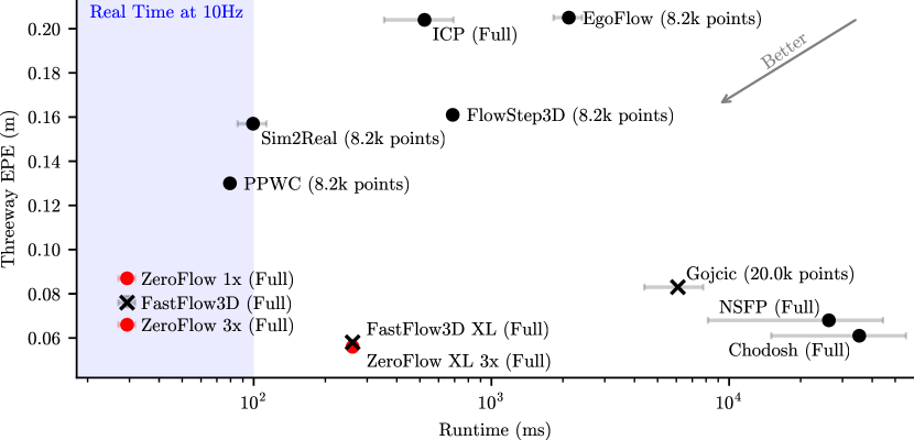
We propose Scene Flow via Distillation (SFvD), a simple, scalable distillation framework that uses a label-free optimization method to produce pseudo-labels to supervise a feedforward model. SFvD generates a new class of scene flow estimation methods that combine the strengths of optimization-based and feedforward methods with the power of data scale and diversity to achieve fast run-time and superior accuracy without human supervision. We instantiate this pipeline into Zero-Label Scalable Scene Flow (ZeroFlow), a family of methods that, motivated by real-world applications, can process full-size point clouds while providing high quality scene flow estimates. We demonstrate the strength of ZeroFlow on Argoverse 2 (Wilson et al., 2021) and Waymo Open (Sun et al., 2020), notably achieving state-of-the-art on the Argoverse 2 Self-Supervised Scene Flow Challenge (Figure 1).

Figure 1: We plot the error and run-time of recent scene flow methods on the Argoverse 2 Sensor dataset (Wilson et al., 2021), along with the size of the point cloud prescribed in the method’s evaluation protocol. Our method ZeroFlow 3X (ZeroFlow trained on 3$\times$ pseudo-labeled data) outperforms its teacher (NSFP, Li et al. (2021b)) while running over 1000$\times$ faster, and ZeroFlow XL 3X (ZeroFlow with a larger backbone trained on 3$\times$ pseudo-labeled data) achieves state-of-the-art. Methods that use any human labels are plotted with , and zero-label methods are plotted with .

Our primary contributions include:

• We introduce a simple yet effective distillation framework, Scene Flow via Distillation (SFvD), which uses a label-free optimization method to produce pseudo-labels to supervise a feedforward model, allowing us to surpass the performance of slow optimization-based approaches at the speed of feedforward methods.

• Using SFvD, we present Zero-Label Scalable Scene Flow (ZeroFlow), a family of methods that produce fast, state-of-the-art scene flow on full-size clouds, with methods running over 1000$\times$ faster than state-of-the-art optimization methods (29.33 ms for ZeroFlow 1X vs 35,281.4 ms for Chodosh) on real point clouds, while being over 1000$\times$ cheaper to train compared to the cost of human annotations ($394 vs $\sim$$750,000).

• We release high quality flow pseudo-labels (representing 7.1 GPU months of compute) for the popular Argoverse 2 (Wilson et al., 2021) and Waymo Open (Sun et al., 2020) autonomous vehicle datasets, alongside our code and trained model weights, to facilitate further research.

2 Background and Related Work

Given point clouds $P_{t}{}$ at time $t$ and $P_{t+1}{}$ at time $t+1$, scene flow estimators predict $\hat{F}_{t,t+1}{}$, a 3D vector for each point in $P_{t}$ that describes how it moved from $t$ to $t+1$ (Dewan et al., 2016). Performance is traditionally measured using the Endpoint Error (EPE) between the predicted flow $\hat{F}_{t,t+1}{}$ and ground truth flow $F^{*}_{t,t+1}{}$ (Equation 1):

$$\textup{EPE}\left({P_{t}}\right)=\frac{1}{\left\lVert P_{t}\right\rVert}\sum_{p\in P_{t}}\left\lVert\hat{F}_{t,t+1}{}(p)-F^{*}_{t,t+1}{}(p)\right\rVert_{2}.$$ (1)

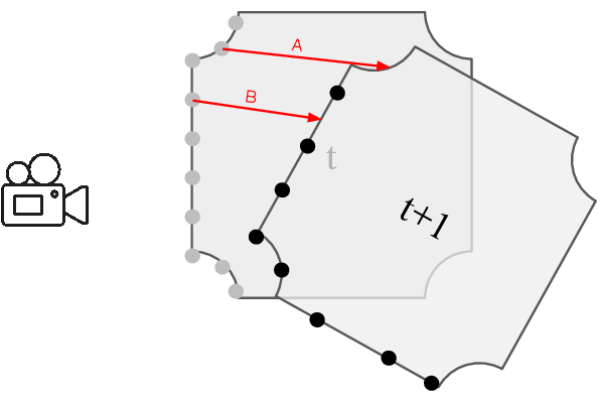
Unlike next token prediction in language (Radford et al., 2018) or next frame prediction in vision (Weng et al., 2021), future observations do not provide ground truth scene flow (Figure 2). To simply evaluate scene flow estimates, ground truth motion descriptions must be provided by an oracle, typically human annotation of real data (Sun et al., 2020; Wilson et al., 2021) or the generator of synthetic datasets (Mayer et al., 2016; Zheng et al., 2023).

Figure 2: Scene Flow vectors describe where the point on an object at time $t$ will end up on the object at $t+1$. In this example, ground truth flow vector A, associated with a point in the upper left concave corner of the object at $t$ has no nearby observations at $t+1$ due to occlusion of the concave feature. The ground truth flow vector B, associated with a point on the face of the object at $t$, does not directly match with any observed point on the object at $t+1$ due to observational sparsity. Thus, point matching between $t$ and $t+1$ alone is insufficient to generate ground truth flow.

Recent scene flow estimation methods either train feedforward methods via supervision from human annotations (Liu et al., 2019; Behl et al., 2019; Tishchenko et al., 2020; Kittenplon et al., 2021; Wu et al., 2020; Puy et al., 2020; Li et al., 2021a; Jund et al., 2021; Gu et al., 2019; Battrawy et al., 2022; Wang et al., 2022), perform human-designed test-time surrogate objective optimization over hand-designed representations (Pontes et al., 2020; Eisenberger et al., 2020; Li et al., 2021b; Chodosh et al., 2023), or learn from self-supervision from human-designed surrogate objectives (Mittal et al., 2020; Baur et al., 2021; Gojcic et al., 2021; Dong et al., 2022; Li et al., 2022).

Supervised feedforward methods are efficient at test-time; however, they require costly human annotations at train-time. Both test-time optimization and self-supervised feedforward methods seek to address this problem by optimizing or learning against label-free surrogate objectives, e.g. Chamfer distance (Pontes et al., 2020), cycle-consistency (Mittal et al., 2020), and various hand-designed rigidity priors (Dewan et al., 2016; Pontes et al., 2020; Li et al., 2022; Chodosh et al., 2023; Baur et al., 2021; Gojcic et al., 2021). Self-supervised methods achieve faster inference by forgoing expensive test-time optimization, but do not match the quality of optimization-based methods (Chodosh et al., 2023) and tend to require human-designed priors via more sophisticated network architectures compared to supervised methods (Baur et al., 2021; Gojcic et al., 2021; Kittenplon et al., 2021). In practice, this makes them slower and more difficult to train. In contrast to existing work, we take advantage of the quality of optimization-based methods as well as the efficiency and architectural simplicity of supervised networks. Our approach, ZeroFlow, uses label-free optimization methods (Li et al., 2021b) to produce pseudo-labels to supervise a feedforward model (Jund et al., 2021).

3 Method

Figure 3: The Scene Flow via Distillation (SFvD) framework, which describes a new class of scene flow methods that produce high quality, human label-free flow at the speed of feedforward networks.

We propose Scene Flow via Distillation (SFvD), a simple, scalable distillation framework that creates a new class of scene flow estimators by using a label-free optimization method to produce pseudo-labels to supervise a feedforward model (Figure 3). While conceptually simple, efficiently instantiating SFvD requires careful construction; most online optimization methods and feedforward architectures are unable to efficiently scale to full-size point clouds (Section 3.1).

Based on our scalability analysis, we propose Zero-Label Scalable Scene Flow (ZeroFlow), a family of scene flow models based on SFvD that produces fast, state-of-the-art scene flow estimates for full-size point clouds without any human labels (Algorithm 1). ZeroFlow uses Neural Scene Flow prior (NSFP) (Li et al., 2021b) to generate high quality, label-free pseudo-labels on full-size point clouds (Section 3.2) and FastFlow3D (Jund et al., 2021) for efficient inference (Section 3.3).

3.1 Scaling Scene Flow via Distillation to Large Point Clouds

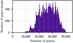
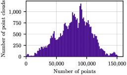
Popular AV datasets including Argoverse 2 (Wilson et al. (2021), collected with dual Velodyne VLP-32 sensors) and Waymo Open (Sun et al. (2020), collected with a proprietary lidar sensor and subsampled) have full-size point clouds with an average of 52,000 and 79,000 points per frame, respectively, after ground plane removal (Supplemental A, Figure 6). For practical applications, sensors such as the Velodyne VLP-128 in dual return mode produce up to 480,000 points per sweep (Vel, 2019) and proprietary sensors at full resolution can produce well over 1 million points per sweep. Thus, scene flow methods must be able to process many points in real-world applications.

Unfortunately, most existing methods focus strictly on scene flow quality for toy-sized point clouds, constructed by randomly subsampling full point clouds down to 8,192 points (Jin et al., 2022; Tishchenko et al., 2020; Wu et al., 2020; Kittenplon et al., 2021; Liu et al., 2019; Li et al., 2021b). As we are motivated by real-world applications, we instead target scene flow estimation for the full-sized point cloud, making architectural efficiency of paramount importance. As an example of stark differences between feedforward architectures, FastFlow3D (Jund et al., 2021), which uses a PointPillar-style encoder (Lang et al., 2019), can process 1 million points in under 100 ms on an NVIDIA Tesla P1000 GPU (making it real-time for a 10Hz LiDAR), while methods like FlowNet3D (Liu et al., 2019) take almost 4 seconds to process the same point cloud.

We design our approach to efficiently process full-size point clouds. For SFvD’s pseudo-labeling step, speed is less of a concern; pseudo-labeling each point cloud pair is offline and highly parallelizable. High-quality methods like Neural Scene Flow Prior (NSFP, Li et al. (2021b)) require only a modest amount of GPU memory (under $3$GB) when estimating scene flow on point clouds with 70K points, enabling fast and low-cost pseudo-labeling using a cluster of commodity GPUs; as an example, pseudo-labeling the Argoverse 2 train split with NSFP is over 1000$\times$ cheaper than human annotation (Supplemental E). The efficiency of SFvD’s student feedforward model is critical, as it determines both the method’s test-time speed and its training speed (faster training enables scaling to larger datasets), motivating models that can efficiently process full-size point clouds.

3.2 Neural Scene Flow Prior is a Slow Teacher

Neural Scene Flow Prior (NSFP, Li et al. (2021b)) is an optimization-based approach to scene flow estimation. Notably, it does not use ground truth labels to generate high quality flows, instead relying upon strong priors in its learnable function class (determined by the coordinate network’s architecture) and optimization objective (Equation 2). Point residuals are fit per point cloud pair $P_{t}$, $P_{t+1}{}$ at test-time by randomly initializing two MLPs; one to describe the forward flow $\hat{F}^{+}$ from $P_{t}$ to $P_{t+1}{}$, and one to describe the reverse flow $\hat{F}^{-}$ from $P_{t}{}+\hat{F}_{t,t+1}$ to $P_{t}{}$ in order to impose cycle consistency. The forward flow $\hat{F}^{+}$ and backward flow $\hat{F}^{-}$ are optimized jointly to minimize

$$\textup{TruncatedChamfer{}}(P_{t}{}+\hat{F}^{+},P_{t+1})+\textup{TruncatedChamfer{}}(P_{t}{}+\hat{F}^{+}+\hat{F}^{-},P_{t})\enspace,$$ (2)

where TruncatedChamfer is the standard Chamfer distance with per-point distances above 2 meters set to zero to reduce the influence of outliers.

NSFP is able to produce high-quality scene flow estimations due to its choice of coordinate network architecture and use of cycle consistency constraint. The coordinate network’s learnable function class is expressive enough to fit the low frequency signal of residuals for moving objects while restrictive enough to avoid fitting the high frequency noise from TruncatedChamfer, and the cycle consistency constraint acts as a local smoothness regularizer for the forward flow, as any shattering effects in the forward flow are penalized by the backwards flow. NSFP provides high quality estimates on full-size point clouds (Figure 1), so we select NSFP for ZeroFlow’s pseudo-label step of SFvD.

3.3 FastFlow3D is a Fast Student

FastFlow3D (Jund et al., 2021) is an efficient feedforward method that learns using human supervisory labels $F^{*}_{t,t+1}{}$ and per-point foreground / background class labels. FastFlow3D’s loss minimizes a variation of the End-Point Error (Equation 1) that reduces the importance of annotated background points, thus minimizing

$$\!\frac{1}{\left\lVert P_{t}\right\rVert}\sum_{p\in P_{t}}\!\sigma(p)\left\lVert\hat{F}_{t,t+1}{}(p)-F^{*}_{t,t+1}{}(p)\right\rVert_{2}$$ (3)

where

$$\sigma(p)=\begin{cases}1&\text{if }p\in\text{Foreground}\\ 0.1&\text{if }p\in\text{Background}\enspace.\end{cases}$$ (4)

FastFlow3D’s architecture is a PointPillars-style encoder (Lang et al., 2019), traditionally used for efficient LiDAR object detection (Vedder & Eaton, 2022), that converts the point cloud into a birds-eye-view pseudoimage using infinitely tall voxels (pillars). This pseudoimage is then processed with a 4 layer U-Net style backbone. The encoder of the U-Net processes the $P_{t}$ and $P_{t+1}$ pseudoimage separately, and the decoder jointly processes both pseudoimages. A small MLP is used to decode flow for each point in $P_{t}{}$ using the point’s coordinate and its associated pseudoimage feature.

As discussed in Section 3.1, FastFlow3D’s architectural design choices make fast even on full-size point clouds. While most feedforward methods are evaluated using a standard toy evaluation protocol with subsampled point clouds, FastFlow3D is able to scale up to full resolution point clouds while maintaining real-time performance and emitting competitive quality scene flow estimates using human supervision, making it a good candidate for the distillation step of SFvD.

In order to train FastFlow3D using pseudo-labels, we replace the foreground / background scaling function (Equation 4) with a simple uniform weighting ($\sigma(\cdot)=1$), which collapses to Average EPE; see Supplemental B for experiments with other weighting schemes. Additionally, we depart from FastFlow3D’s problem setup in two minor ways: we delete ground points using dataset provided maps, a standard pre-processing step (Chodosh et al., 2023), and use the standard scene flow problem setup of predicting flow between two frames (Section 2) instead of predicting future flow vectors in meters per second. Algorithm 1 describes our approach, with details specified in Section 4.1.

In order to take advantage of the unlabeled data scaling of SFvD, we expand FastFlow3D to a family of models by designing a higher capacity backbone, producing FastFlow3D XL. This larger backbone halves the size of each pillar to quadruple the pseudoimage area, doubles the size of the pillar embedding, and adds an additional layer to maintain the network’s receptive field in metric space; as a result, the total parameter count increases from 6.8 million to 110 million.

Algorithm 1 ZeroFlow

1:$D\leftarrow$ collection of unlabeled point cloud pairs $\triangleright$ Training Data

2:for $P_{t},P_{t+1}\in D$ do$\triangleright$ Parallel For

3:     $F^{*}_{t,t+1}\leftarrow\textup{Teacher{NSFP}}(P_{t},P_{t+1})$ $\triangleright$ SFvD Pseudo-label Step

4:for epoch $\in$ epochs do

5:     for $P_{t},P_{t+1},F^{*}_{t,t+1}\in D$ do $\triangleright$ SFvD’s Distill Step

6:         $l\leftarrow\textup{Equation~{}\ref{equation:fastflowloss}}(\textup{StudentFastFlow3D}_{\theta}(P_{t},P_{t+1}),F^{*}_{t,t+1})$

7:         $\theta\leftarrow\theta$ updated w.r.t. $l$      

4 Experiments

ZeroFlow provides a family of fast, high quality scene flow estimators. In order to validate this family and understand the impact of components in the underlying Scene Flow via Distillation framework, we perform extensive experiments on the Argoverse 2 (Wilson et al., 2021) and Waymo Open (Sun et al., 2020) datasets. We compare to author implementations of NSFP (Li et al., 2021b) and  Chodosh et al. (2023), implement FastFlow3D (Jund et al., 2021) ourselves (no author implementation is available), and use Chodosh et al. (2023)’s implementations for all other baselines.

As discussed in Chodosh et al. (2023), downstream applications typically rely on good quality scene flow estimates for foreground points. Most scene flow methods are evaluated using average Endpoint Error (EPE, Equation 1); however, roughly 80% of real-world point clouds are background, causing average EPE to be dominated by background point performance. To address this, we use the improved evaluation metric proposed by Chodosh et al. (2023), Threeway EPE:

$$\textup{Threeway EPE}(P_{t})=\textup{Avg}\begin{cases}\textup{EPE}({p\in P_{t}:p\in\textup{Background}})&\textup{(Static BG)}\\ \textup{EPE}({p\in P_{t}:p\in\textup{Foreground}\land F^{*}_{t,t+1}{}(p)\leq 0.5\textup{m/s}})&\textup{(Static FG)}\\ \textup{EPE}({p\in P_{t}:p\in\textup{Foreground}\land F^{*}_{t,t+1}{}(p)>0.5\textup{m/s}})&\textup{(Dynamic FG)}\enspace.\\ \end{cases}$$ (5)

4.1 How does ZeroFlow perform compared to prior art on real point clouds?

The overarching promise of ZeroFlow is the ability to build fast, high quality scene flow estimators that improve with the the availability of large-scale unlabeled data. Does ZeroFlow deliver on this promise? How does it compare to state-of-the-art methods?

To characterize the ZeroFlow family’s performance, we use Argoverse 2 to perform scaling experiments along two axes: dataset size and student size. For our standard size configuration, we use the Argoverse 2 Sensor train split and the standard FastFlow3D architecture, enabling head-to-head comparisons against the fully supervised FastFlow3D as well as other baseline methods. For our scaled up dataset (denoted 3X in all experiments), we use the Argoverse 2 Sensor train split and concatenate a roughly twice as large set of unannotated frame pairs from the Argoverse 2 LiDAR dataset, uniformly sampled from its 20,000 sequences to maximize data diversity. For our scaled up student architecture (denoted XL in all experiments), we use the XL backbone described in Section 3.3. For details on the exact dataset construction and method hyperparameters, see Supplemental A

Table 1: Quantitative results on the Argoverse 2 Sensor validation split using the evaluation protocol from Chodosh et al. (2023). The methods used in this paper, shown in the first two blocks of the table, are trained and evaluated on point clouds within a 102.4m $\times$ 102.4m area centered around the ego vehicle (the settings for the Argoverse 2 Self-Supervised Scene Flow Challenge) . However, following the protocol of Chodosh et al. (2023), all methods report error on points in the 70m $\times$ 70m area centered around the ego vehicle. Runtimes are collected on an NVIDIA V100 with a batch size of 1 (Peri et al., 2023). FastFlow3D, ZeroFlow 1X, and ZeroFlow 3X have identical feedforward architectures and thus share the same real-time runtime; FastFlow3D XL, ZeroFlow XL 1X, and ZeroFlow XL 3X have identical feedforward architectures and thus share the same runtime. Methods with an * have performance averaged over 3 training runs (see Supplemental C for details). Underlined methods require human supervision.

	Runtime (ms)		Point Cloud	Threeway	Dynamic	Static	Static
			Subsampled Size	EPE	FG EPE	FG EPE	BG EPE
FastFlow3D* (Jund et al., 2021)	${29.33\pm}$	${2.38}$	Full Point Cloud	0.076	0.186	0.021	0.021
ZeroFlow 1X* (Ours)			Full Point Cloud	0.092	0.231	0.022	0.022
ZeroFlow 3X (Ours)			Full Point Cloud	0.066	0.164	0.017	0.017
FastFlow3D XL	${260.61\pm}$	${1.21}$	Full Point Cloud	0.058	0.139	0.018	0.018
ZeroFlow XL 1X (Ours)			Full Point Cloud	0.072	0.178	0.019	0.019
ZeroFlow XL 3X (Ours)			Full Point Cloud	0.056	0.131	0.018	0.018
NSFP w/ Motion Comp (Li et al., 2021b)	$26,285.0\pm$	$18,139.3$	Full Point Cloud	0.068	0.131	0.036	0.036
Chodosh et al. (Chodosh et al., 2023)	$35,281.4\pm$	$20,247.7$	Full Point Cloud	0.061	0.129	0.028	0.028
Odometry	—		Full Point Cloud	0.198	0.583	0.010	0.000
ICP (Chen & Medioni, 1992)	$523.11\pm$	$169.34$	Full Point Cloud	0.204	0.557	0.025	0.028
Gojcic (Gojcic et al., 2021)	$6,087.87\pm$	$1,690.56$	$20000$	0.083	0.155	0.064	0.032
Sim2Real (Jin et al., 2022)	$99.35\pm$	$13.88$	$8192$	0.157	0.229	0.106	0.137
EgoFlow (Tishchenko et al., 2020)	$2,116.34\pm$	$292.32$	$8192$	0.205	0.447	0.079	0.090
PPWC (Wu et al., 2020)	$79.43\pm$	$2.20$	$8192$	0.130	0.168	0.092	0.129
FlowStep3D (Kittenplon et al., 2021)	$687.54\pm$	$3.13$	$8192$	0.161	0.173	0.132	0.176

As shown in Table 1, ZeroFlow is able to leverage scale to deliver superior performance. While ZeroFlow 1X loses a head-to-head competition against the human-supervised FastFlow3D on both Argoverse 2 (Table 1) and Waymo Open (Table 2), scaling the distillation process to additional unlabeled data provided by Argoverse 2 enables ZeroFlow 3X to significantly surpass the performance of both methods just by training on more pseudo-labled data. ZeroFlow 3X even surpasses the performance of its own teacher, NSFP, while running in real-time!

ZeroFlow’s pipeline also benefits from scaling up the student architecture. We modify ZeroFlow’s architecture with the much larger XL backbone, and show that our ZeroFlow XL 3X is able to combine the power of dataset and model scale to outperform all other methods, including significantly outperform its own teacher. Our simple approach achieves state-of-the-art on both the Argoverse 2 validation split and Argoverse 2 Self-Supervised Scene Flow Challenge.

Table 2: Quantitative results on Waymo Open using the evaluation protocol from Chodosh et al. (2023). Runtimes are scaled to approximate the performance on a V100 (Li et al., 2020). Both FastFlow3D and ZeroFlow 1X have identical feedforward architectures and thus share the same runtime. Underlined methods require human supervision.

	Runtime (ms)		Point Cloud	Threeway	Dynamic	Static	Static
			Subsampled Size	EPE	FG EPE	FG EPE	BG EPE
ZeroFlow 1X (Ours)	$21.66\pm$	$0.48$	Full Point Cloud	0.083	0.216	0.016	0.017
FastFlow3D (Jund et al., 2021)			Full Point Cloud	0.075	0.195	0.015	0.016
Chodosh (Chodosh et al., 2023)	$93,752.3\pm$	$76,786.1$	Full Point Cloud	0.041	0.073	0.013	0.039
NSFP Li et al. (2021b)	$90,999.1\pm$	$74,034.9$	Full Point Cloud	0.100	0.171	0.022	0.108
ICP (Chen & Medioni, 1992)	$302.70\pm$	$157.61$	Full Point Cloud	0.192	0.498	0.022	0.055
Gojcic Gojcic et al. (2021)	$501.69\pm$	$54.63$	20000	0.059	0.107	0.045	0.025
EgoFlow (Tishchenko et al., 2020)	$893.68\pm$	$86.55$	8192	0.183	0.390	0.069	0.089
Sim2Real (Jin et al., 2022)	$72.84\pm$	$14.79$	8192	0.166	0.198	0.099	0.201
PPWC (Wu et al., 2020)	$101.43\pm$	$5.48$	8192	0.132	0.180	0.075	0.142
FlowStep3D (Kittenplon et al., 2021)	$872.02\pm$	$6.24$	8192	0.169	0.152	0.123	0.232

4.2 How does ZeroFlow scale?

Section 4.1 demonstrates that ZeroFlow can leverage scale to capture state-of-the-art performance. However, it’s difficult to perform extensive model tuning for large training runs, so predictable estimates of performance as a function of dataset size are critical (OpenAI, 2023). Does ZeroFlow’s performance follow predictable scaling laws?

We train ZeroFlow and FastFlow3D on sequence subsets / supersets of the Argoverse 2 Sensor train split. Figure 4 shows ZeroFlow and FastFlow3D’s validation Threeway EPE both decrease roughly logarithmically, and this trend appears to hold for XL backbone models as well.

Figure 4: Empirical scaling laws for ZeroFlow. We report Argoverse 2 validation split Threeway EPE as a percentage of the Argoverse 2 train split used, on a log₁₀-log₁₀ scale, trained to convergence. Threeway EPE performance of ZeroFlow scales logarithmically with the amount of training data.

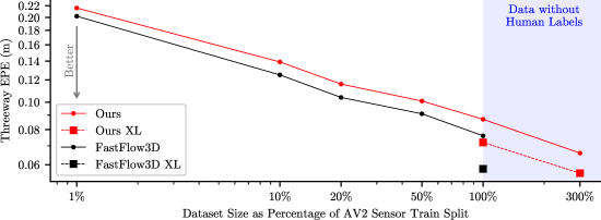
Empirically, ZeroFlow adheres to predictable scaling laws that demonstrate more data (and more parameters) are all you need to get better performance. This makes ZeroFlow a practical pipeline for building scene flow foundation models (Bommasani et al., 2021) using the raw point cloud data that exists today in the deployment logs of Autonomous Vehicles and other deployed systems.

4.3 How does dataset diversity influence ZeroFlow’s performance?

In typical human annotation setups, a point cloud sequence is given to the human annotator. The human generates box annotations in the first frame, and then updates the pose of those boxes as the objects move through the sequence, introducing and removing annotations as needed. This process is much more efficient than annotating disjoint frame pairs, as it amortizes the time spent annotating most objects in the sequence. This is why most human annotated training datasets (e.g. Argoverse 2 Sensor, Waymo Open) are composed of contiguous sequences. However, contiguous frames have significant structural similarity; in the 150 frames (15 seconds) of an Argoverse 2 Sensor sequence, the vehicle typically observes no more than a city block’s worth of unique structure. ZeroFlow, which requires zero human labels, does not have this constraint on its pseudo-labels; NSFP run on non-sequential frames is no more expensive than NSFP run on non-sequential frames, enabling ZeroFlow to train on a more diverse dataset. How does dataset diversity impact performance?

To understand the impact of data diversity, we train a version of ZeroFlow 1X and ZeroFlow 2X only on the diverse subset of our Argoverse 2 LiDAR data selected by uniformly sampling 12 frame pairs from each of the 20,000 unique sequences (Table 3).

Table 3: Comparison between ZeroFlow trained on Argoverse 2 Sensor dataset versus the more diverse, unlabeled Argoverse 2 LiDAR subset described in Section 4.1. Diverse training datasets result in non-trivial performance improvements.

	Threeway	Dynamic	Static	Static
	EPE	FG EPE	FG EPE	BG EPE
FastFlow3D* (Jund et al., 2021)	$0.076$	$0.186$	$0.021$	$0.021$
ZeroFlow 1X (AV2 Sensor Data)*	$0.092$	$0.231$	$0.022$	$0.022$
ZeroFlow 1X (AV2 LiDAR Subset Data)	$0.085$	$0.218$	$0.018$	$0.018$
ZeroFlow 2X (AV2 LiDAR Subset Data)	$0.076$	$0.184$	$0.022$	$0.022$

Dataset diversity has a non-trivial impact on performance; ZeroFlow, by virtue of being able to learn across non-contiguous frame pairs, is able to see more unique scene structure and thus learn to better to extract motion in the presence of the unique geometries of the real world.

4.4 How do the noise characteristics of ZeroFlow compare to other methods?

ZeroFlow distills NSFP into a feedforward model from the FastFlow3D family. Section 4.1 highlights the average performance of ZeroFlow across Threeway EPE catagories, but what does the error distribution look like?

(a) FastFlow3D, Log

(b) ZeroFlow 1X, Log

(c) ZeroFlow 3X, Log

(d) ZeroFlow XL 3X, Log

(e) NSFP, Log

(f) Chodosh, Log

(g) FastFlow3D, Abs.

(h) ZeroFlow 1X, Abs.

(i) ZeroFlow 3X, Abs.

(j) ZeroFlow XL 3X, Abs.

(k) NSFP, Abs.

(l) Chodosh, Abs.

Figure 5: Normalized frame birds-eye-view heatmaps of endpoint residuals for Chamfer Distance, as well as the outputs for NSFP and Chodosh on moving points (points with ground truth speed above 0.5m/s). Perfect predictions would produce a single central dot. Top row shows the frequency on a $\log_{10}$ color scale, bottom row shows the frequency on an absolute color scale. Qualitatively, methods with better quantitative results have tighter residual distributions. See Supplemental F for details.

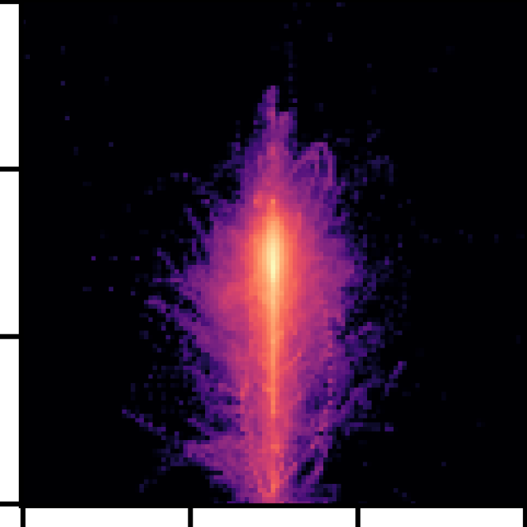
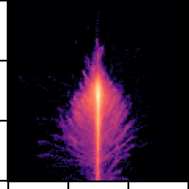
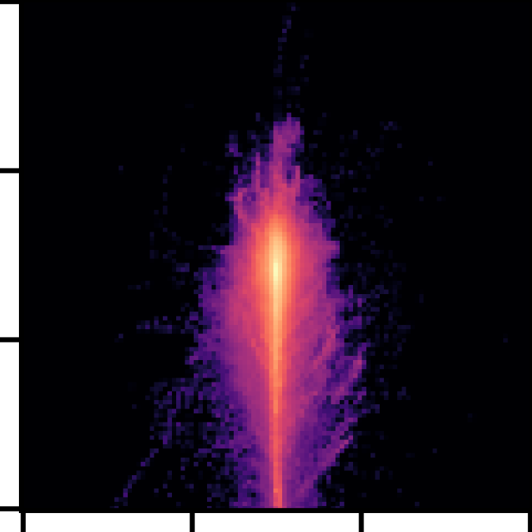
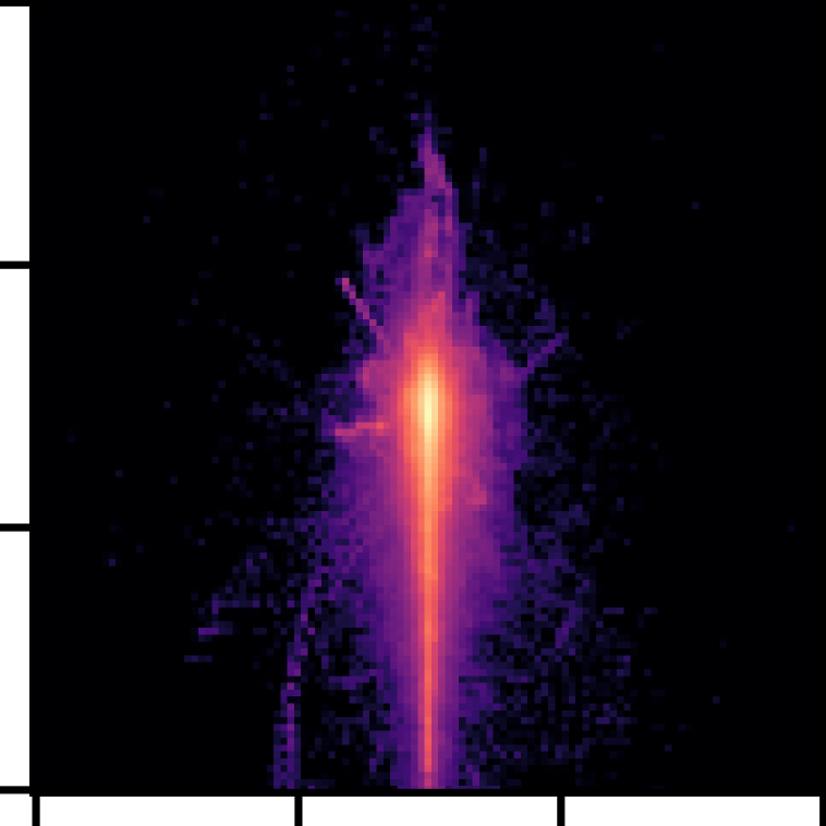
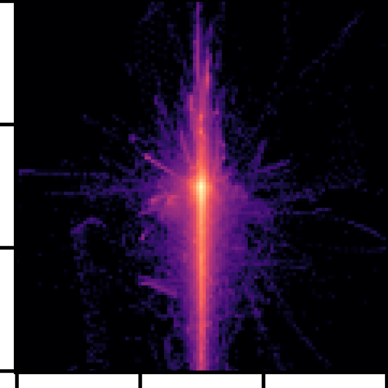
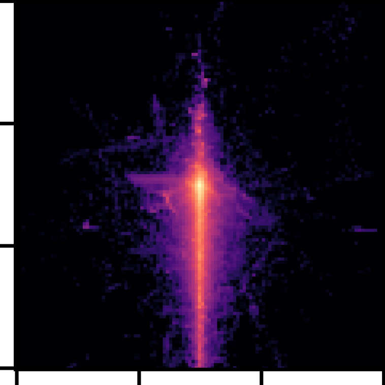
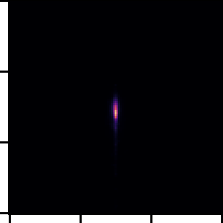
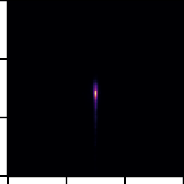
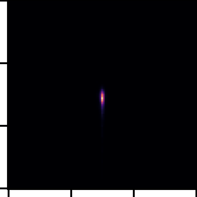
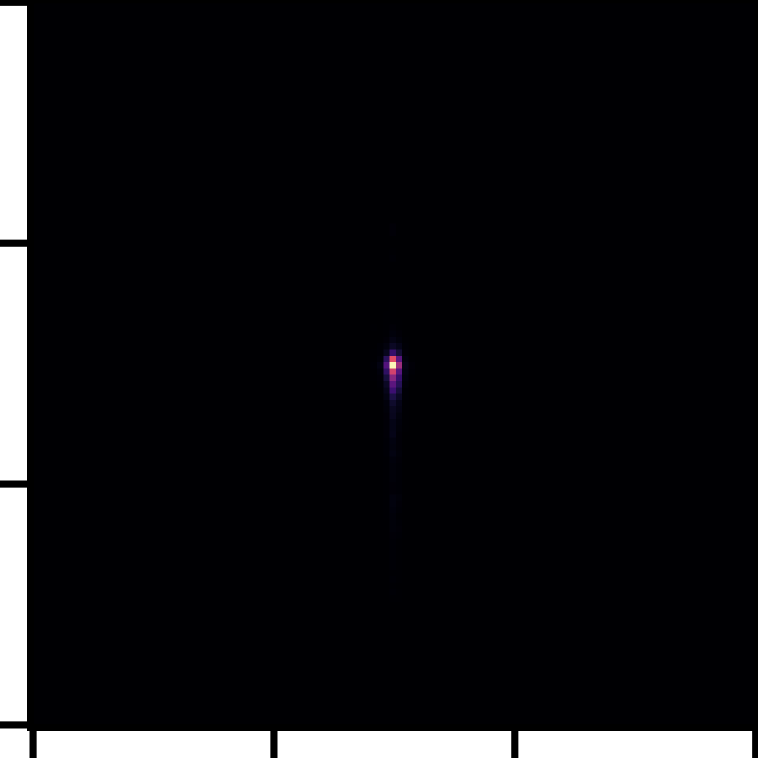
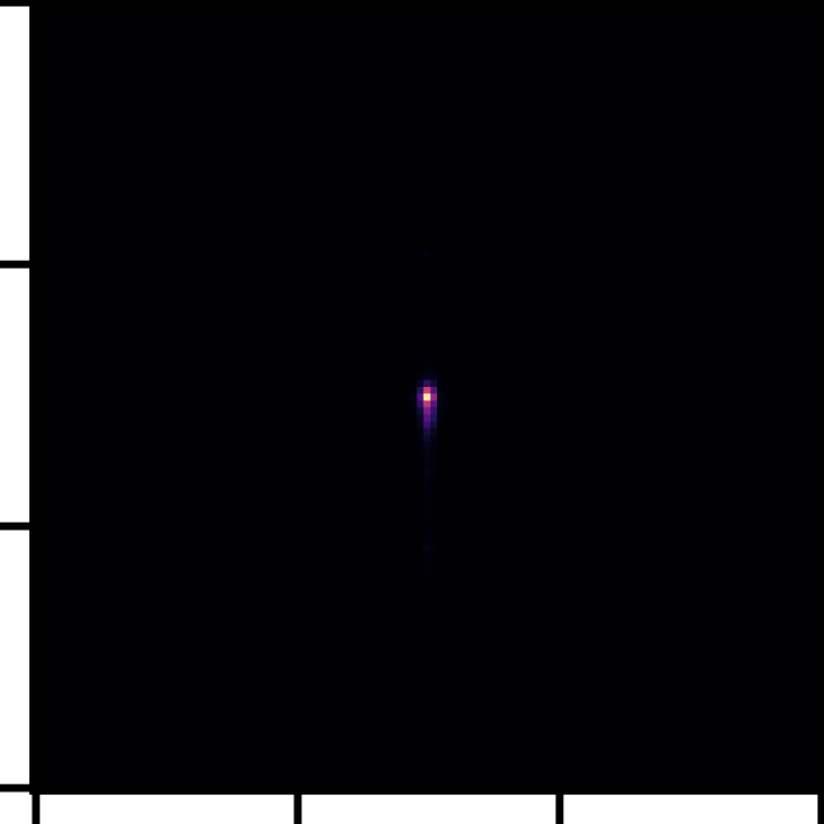
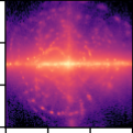
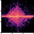
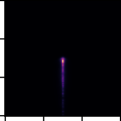
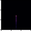
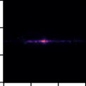
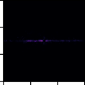
To answer this question, we plot birds-eye-view flow vector residuals of NSFP, Chodosh, FastFlow3D, and several members of the ZeroFlow family on moving objects from the Argoverse 2 validation dataset, where the ground truth is rotated vertically and centered at the origin to present all vectors in the same frame (Figure 5; see Supplemental F for details on construction). Qualitatively, these plots show that error is mostly distributed along the camera ray and distributional tightness ($\log_{10}$ plots) roughly corresponds to overall method performance.

Overall, these plots provide useful insights to practitioners and researchers, particularly for consumption in downstream tasks; as an example, open world object extraction (Najibi et al., 2022) requires the ability to threshold for motion and cluster motion vectors together to extract the entire object. Decreased average EPE is useful for this task, but understanding the magnitude and distribution of flow vectors is needed to craft good extraction heuristics.

4.5 How does teacher quality impact ZeroFlow’s performance?

As shown in Section 4.1  (Chodosh et al., 2023) has superior Threeway EPE over NSFP on both Argoverse 2 and Waymo Open. Can a better performing teacher lead a better version of ZeroFlow?

To understand the impact of a better teacher, we train ZeroFlow on Argoverse 2 using superior quality flow vectors from Chodosh et al. (2023), which proposes a refinement step to NSFP lablels to provide improvements to flow vector quality (Table 4). ZeroFlow trained on Chodosh refined pseudo-labels provides no meaningful quality improvement over NSFP pseudo-labels (as discussed in Supplemental C, a Threeway EPE difference of $0.2$cm is within training variance for ZeroFlow). These results also hold for our ablated speed scaled version of ZeroFlow in Supplemental B.

Since increasing the quality of the teacher over NSFP provides no noticeable benefit, can we get away with using a significantly faster but lower quality teacher to replace NSFP, e.g. the commonly used self-supervised proxy of TruncatedChamfer?

To understand if NSFP is necessary, we train ZeroFlow on Argoverse 2 using pseudo-labels from the nearest neighbor, truncated to 2 meters as with TruncatedChamfer. The residual distribution of TruncatedChamfer is shown in Supplemental F, Figure 10(a). ZeroFlow trained on TruncatedChamfer pseudo-labels performs significantly worse than NSFP, motivating the use of NSFP as a teacher.

Table 4: Comparison between ZeroFlow trained on Argoverse 2 using NSFP pseudo-labels, ZeroFlow using Chodosh et al. (2023) pseudo-labels, and ZeroFlow using TruncatedChamfer. Methods with an * have performance averaged over 3 training runs (see Supplemental C for details). The minor quality improvement of Chodosh pseudo-labels does not lead to a meaningful difference in performance, while the significant degradation of TruncatedChamfer leads to significantly worse performance.

	Threeway	Dynamic	Static	Static
	EPE	FG EPE	FG EPE	BG EPE
ZeroFlow 1X (NSFP pseudo-labels)*	$0.092$	$0.231$	$0.022$	$0.022$
ZeroFlow 1X (Chodosh et al. (2023) pseudo-labels)	$0.090$	$0.234$	$0.018$	$0.018$
ZeroFlow 1X (TruncatedChamfer pseudo-labels)	$0.108$	$0.226$	$0.049$	$0.049$

5 Conclusion

Our scene flow approach, Zero-Label Scalable Scene Flow (ZeroFlow), produces fast, state-of-the-art scene flow without human labels via our conceptually simple distillation pipeline.

But, more importantly, we present the first practical pipeline for building scene flow foundation models (Bommasani et al., 2021) using the raw point cloud data that exists today in the deployment logs at Autonomous Vehicle companies and other deployed robotics systems. Foundational models in other domains like language (Brown et al., 2020; OpenAI, 2023) and vision (Kirillov et al., 2023; Rajeswaran et al., 2022) have enabled significant system capabilities with little or no additional domain-specific fine-tuning (Wang et al., 2023; Ma et al., 2022; 2023). We posit that a scene flow foundational model will enable new systems that can leverage high quality, general scene flow estimates to robustly reason about object dynamics even in foreign or noisy environments.

Limitations and Future Work. ZeroFlow inherits the biases of its pseudo-labels. Unsurprisingly, if the pseudo-labels consistently fail to estimate scene flow for certian objects, our method will also be unable to predict scene flow for those objects; however, further innovation in model architecture, loss functions, and pseudo-labels may yield better performance. In order to enable further work on Scene Flow via Distillation-based methods, we release our code, trained model weights, and NSFP flow pseudo-labels, representing $3.6$ GPU months for Argoverse 2 and $3.5$ GPU months for Waymo Open.

Acknowledgements. The research presented in this paper was partially supported by the DARPA SAIL-ON program under contract HR001120C0040, the DARPA ShELL program under agreement HR00112190133, the Army Research Office under MURI grant W911NF20-1-0080, and the CMU Center for Autonomous Vehicle Research.

Appendix A Argoverse 2 and Waymo Open Dataset Configuration Details

Argoverse 2. The Sensor dataset contains 700 training and 150 validation sequences. Each sequence contains 15 seconds of 10Hz point clouds collected using two Velodyne VLP-32s mounted on the roof of a car. As part of the training protocol for ZeroFlow, FastFlow3D, and NSFP w/ Motion Compensation, we perform ego compensation, ground point removal, and restrict all points to be within a 102.4m $\times$ 102.4m area centered around the ego vehicle, resulting in point clouds with an average of 52,871 points (Figure 6(a)). The point cloud $P_{t+1}{}$ is centered at the origin of the ego vehicle’s coordinate system and $P_{t}{}$ is projected into $P_{t+1}{}$’s coordinate frame. For ZeroFlow and FastFlow3D, the PointPillars encoder uses $0.2$m$\times 0.2$m pillars, with all architectural configurations matching (Jund et al., 2021). For NSFP w/ Motion Compensation, we use the same architecture and early stopping parameters as the original method (Li et al., 2021b). For FastFlow3D and the FastFlow3D student architecture of ZeroFlow, we train to convergence (50 epochs) with an Adam (Kingma & Ba, 2014) learning rate of $2\text{\times}{10}^{-6}\text{\,}\mathrm{a}$nd batch size $64$. For FastFlow3D XL and the FastFlow3D XL student architecture of ZeroFlow (ZeroFlow XL 1X, ZeroFlow XL 3X), we train to convergence (10 epochs) with the same optimizer settings and a batch size $12$. For ZeroFlow 3X and and ZeroFlow XL 3X, we train on an additional 240,000 unlabeled frame pairs (roughly twice the size as the Argoverse 2 Sensor train split), constructed by selecting 12 frame pairs at uniform intervals from the 20,000 sequences of the Argoverse 2 LiDAR dataset. For all other methods in Table 1, we use the implementations provided by Chodosh et al. (2023), which follow ground removal and ego compensation protocols from their respective papers.

Waymo Open. The dataset contains 798 training and 202 validation sequences. Each sequence contains 20 seconds of 10Hz point clouds collected using a custom LiDAR mounted on the roof of a car. We use the same preprocessing and training configurations used on Argoverse 2; after ego motion compensation and ground point removal, the average point cloud has 79,327 points (Figure 6(b)).

As shown in Figure 6, Argoverse 2 (Wilson et al., 2021) and Waymo Open (Sun et al., 2020) are significantly larger than the 8,192 point subsampled point clouds used by prior art.

(a) Distribution of point cloud sizes in the Argoverse 2 Sensor val split: $\mu=52,871.6;\sigma=12,227.2$.

(b) Distribution of point cloud sizes in the Waymo Open val split: $\mu=79,327.8;\sigma=27,182.1$.

Figure 6: Point cloud size distributions for the val set of the Argoverse 2 Sensor (Wilson et al., 2021) and Waymo Open (Sun et al., 2020) datasets after ground removal and clipped to a 102.4m $\times$ 102.4m box around the ego vehicle.

Figure 7: Scene flow estimation of two consecutive point clouds sampled 100 ms apart (green and blue, respectively) on Argoverse 2 (Wilson et al., 2021). Left: Ground truth scene flow annotations in red. These annotations are derived from the motion of amodal bounding boxes. Right: ZeroFlow’s scene flow estimates estimates in orange, which closely match with the ground truth.

Appendix B Exploring the importance of point weighting

In order to train FastFlow3D using pseudo-labels, we need a replacement $\sigma(\cdot)$ semantics scaling function described in Equation 4) because our pseudo-labels do not provide foreground / background semantics. In the main experiments, we use uniform scaling ($\sigma(\cdot)=1$).

B.1 Can we design a better point weighting function for pseudo-labels?

We propose a soft weighting based on pseudo-label flow magnitude: for the point $p$ in the pseudo-label flow $F^{*}_{t,t+1}{}(p)$, where $s(p)$ represents its speed in meters per second, we linearly interpolate the weight of $p$ between $0.1\times$ at 0.4 m/s and full weight at 1.0 m/s, i.e.

$$\sigma(p)=\begin{cases}0.1&\text{if }s(p)<0.4\text{ m/s}\\ 1.0&\text{if }s(p)>1.0\text{ m/s}\\ 1.8s-0.8&\text{o.w.}\end{cases}$$ (6)

These thresholds are selected to down-weight approximately 80% of points by $0.1\times$, with the other 20% of points split between the soft and full weight region. In Table 5, we show that our weighting scheme provides non-trivial improvements over uniform weighting (i.e. $\sigma(\cdot)=1$) for ZeroFlow 1X; however, it actually hurts performance for ZeroFlow 3X.

Table 5: Comparison between ZeroFlow trained on Argoverse 2 using NSFP pseudo-labels and ZeroFlow using Chodosh et al. (2023) pseudo-labels using both uniform and speed scaled point weighting. Methods with an * have performance averaged over 3 training runs (see Supplemental C for details).

	Threeway	Dynamic	Static	Static
	EPE	FG EPE	FG EPE	BG EPE
ZeroFlow 1X (Equation 6, NSFP pseudo-labels)*	$0.087$	$0.217$	$0.023$	$0.023$
ZeroFlow 1X (Equation 6, Chodosh et al. (2023) pseudo-labels)	$0.088$	$0.227$	$0.019$	$0.019$
ZeroFlow 1X (NSFP pseudo-labels)*	$0.092$	$0.231$	$0.022$	$0.022$
ZeroFlow 1X (Chodosh et al. (2023) pseudo-labels)	$0.090$	$0.234$	$0.018$	$0.018$
ZeroFlow XL 3X	$0.056$	$0.131$	$0.018$	$0.018$
ZeroFlow XL 3X (Equation 6)	$0.058$	$0.139$	$0.017$	$0.017$

B.2 How much of FastFlow3D’s performance is due to its semantic point weighting?

Unlike ZeroFlow, FastFlow3D can use human foreground / background point labels to upweight the flow importance of foreground points (Section 3.3, Equation 4). To understand the impact of this weighting, we train FastFlow3D with two modified losses; rather than scaling using semantics as described in Equation 4, we uniformly weight all points ($\sigma(\cdot)=1$) or our speed based weighting (Equation 6).

Table 6: Comparison between ZeroFlow, FastFlow3D, and the ablated FastFlow3D with uniform scaling ($\sigma(\cdot)=1$) trained on Argoverse 2. The performance of FastFlow3D with Uniform Scaling and our speed scaling (Equation 6) are nearly identical to ZeroFlow’s performance. Methods with an * have performance averaged over 3 training runs (see Supplemental C for details). Underlined methods require human supervision.

	Threeway	Dynamic	Static	Static
	EPE	FG EPE	FG EPE	BG EPE
ZeroFlow 1X* (Ours)	$0.087$	$0.217$	$0.023$	$0.023$
FastFlow3D ($\sigma(\cdot)=1$)	$0.085$	$0.220$	$0.018$	$0.018$
FastFlow3D (Equation 6)	$0.084$	$0.211$	$0.020$	$0.020$
FastFlow3D* (Jund et al., 2021)	$0.076$	$0.186$	$0.021$	$0.021$

As shown in Table 6, the performance of FastFlow3D ($\sigma(\cdot)=1$) and (Equation 6) degrades almost completely to ZeroFlow’s performance (e.g. $0.076\rightarrow 0.085$, $0.084$ vs $0.087$ for Threeway EPE).

This raises the question: why is the performance improvement of semantic weighting larger than the improvement of our unsupervised moving point weighting scheme (Supplemental B.1)? We conjecture that not only does semantic weighting provide increased loss on moving objects, it implicitly teaches the network to recognize the structure of objects themselves. For example, with Equation 4 scaling, end-point error on a stationary pedestrian is significantly higher than static background points, incentivizing the network to learn to detect the point structure common to pedestrians, even if immobile, to perfect the predictions on those points.

Appendix C Characterizing inter-training run final performance variance for ZeroFlow and FastFlow3D

On Argoverse 2, Threeway EPE difference between ZeroFlow and the human supervised FastFlow3D is $1.6$cm (Table 1); how much of this gap can be attributed to training variance between runs? To answer this question, we train ZeroFlow and FastFlow3D from scratch 3 times each. ZeroFlow is trained on the same Argoverse 2 NSFP pseudo-labels (Table 8), resulting in a mean Threeway EPE of $0.092$m with error of $0.003$m ($0.3$cm) in either direction, and FastFlow3D is trained on the Argoverse 2 human labels (Table 9), resulting in a mean Threeway EPE of $0.092$m with error under $0.003$m ($0.3$cm) in either direction.

To contextualize the scale of this variance, the underlying Velodyne VLP-32 sensors used to collect the Argoverse 2 are only certified to $\pm 3$ cm of error (Lopac et al., 2022) (an order of magnitude greater than the deviation from the mean train performance for ZeroFlow), and this entirely neglects additional sources of noise introduced from other real world effects such as empirical ego motion compensation.

Table 7: Performance of ZeroFlow over 3 train runs on the same NSFP pseudo-labels.

	Threeway	Dynamic	Static	Static
	EPE	FG EPE	FG EPE	BG EPE
ZeroFlow 1X Run #1	$0.089$	$0.224$	$0.021$	$0.021$
ZeroFlow 1X Run #2	$0.092$	$0.231$	$0.022$	$0.022$
ZeroFlow 1X Run #3	$0.095$	$0.240$	$0.023$	$0.023$
ZeroFlow 1X Average	$0.092$	$0.231$	$0.022$	$0.022$

Table 8: Performance of ZeroFlow ablated with point scaling (Equation 6) over 3 train runs on the same NSFP pseudo-labels.

	Threeway	Dynamic	Static	Static
	EPE	FG EPE	FG EPE	BG EPE
ZeroFlow 1X (Equation 6) Run #1	$0.087$	$0.214$	$0.023$	$0.023$
ZeroFlow 1X (Equation 6) Run #2	$0.087$	$0.215$	$0.024$	$0.024$
ZeroFlow 1X (Equation 6) Run #3	$0.089$	$0.222$	$0.022$	$0.022$
ZeroFlow 1X (Equation 6) Average	$0.087$	$0.217$	$0.023$	$0.023$

Table 9: Performance of FastFlow3D over 3 train runs on the Argoverse 2 human labels.

	Threeway	Dynamic	Static	Static
	EPE	FG EPE	FG EPE	BG EPE
FastFlow3D Run #1	$0.074$	$0.181$	$0.020$	$0.020$
FastFlow3D Run #2	$0.076$	$0.186$	$0.021$	$0.021$
FastFlow3D Run #3	$0.079$	$0.191$	$0.023$	$0.023$
FastFlow3D Average	$0.076$	$0.186$	$0.021$	$0.021$

Appendix D Characterizing how ZeroFlow’s performance evolves during training

Threeway EPE breaks down performance into three categories: Foreground Dynamic, Foreground Static, and Background. How does ZeroFlow’s performance evolve during training?

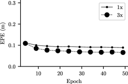
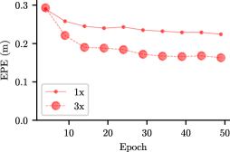
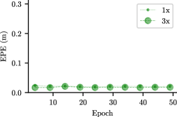
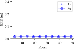
To understand this, we plot ZeroFlow 1X and ZeroFlow 3X in Figure 8. Both methods converge to their final background performance almost immediately, and most of the improvements seen in the final Threeway EPE stem from improvements in Foreground Dynamic (Figure 8(b)). The impact of additional data is also made clear early in training, as ZeroFlow 3X has significantly lower Threeway EPE by epoch 15 than ZeroFlow 1X.

(a) Threeway EPE

(b) Foreground Dynamic

(c) Foreground Static

(d) Background

Figure 8: Performance of ZeroFlow 1X and ZeroFlow 3X on the Argoverse 2 val split by training epoch. Both methods converge to their final background performance almost immediately, and most of the improvements seen in the final Threeway EPE stem from improvements in Foreground Dynamic (Figure 8(b)).

Appendix E Estimating Human Labeling versus Pseudo-labeling costs

NSFP pseudolabeling of the Argoverse 2 train split (700 sequences of 150 frames) required a total of 753 hours of NVidia Turing generation GPU time. At September, 2023 Amazon Web Services EC2 prices, a single g4dn.xlarge, equipped with a single NVidia Tesla T4, costs $0.526 per hour, for a total cost of $394 to pseudo-label. By comparison, at an estimated $0.10 per frame per cuboid (no public cost statements exist for production quality AV dataset labels, but this the standard price point within the industry), Argoverse 2’s train split has an average of 75 cuboids per frame (Wilson et al., 2021), for a total cost on the order of $787,500 to human annotate.

Appendix F Details on Endpoint Residuals

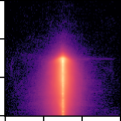
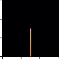
The process of constructing these endpoint residual plots is shown in Figure 9. For moving points (points with a ground truth flow vector magnitude >0.5m/s), the raw points (Figure 9(a)) are transformed into a standard frame with the ground truth vector pointing up and the endpoint at the center of the plot (Figure 9(b)), and the residual endpoints are accumulated (Figure 9(c)). Residual plots for baselines, as well as their unrotated counterparts, are shown in Figure 10.

(a) Raw Points

(b) Standard Frame

(c) Error Dots

Figure 9: Process for constructing the endpoint residual plots. The raw points (Figure 9(a)) are transformed into a standard frame with the ground truth vector pointing up and the endpoint at the center of the plot (Figure 9(b)), and the residual endpoints are accumulated (Figure 9(c)).

(a) Nearest Neighbor, Log, Rotated

(b) $\vec{0}$ Flow, Log, Rotated

(c) Nearest Neighbor, Log, Unrotated

(d) $\vec{0}$ Flow, Log, Unrotated

(e) Nearest Neighbor, Abs, Rotated

(f) $\vec{0}$ Flow, Abs, Rotated

(g) Nearest Neighbor, Abs, Unrotated

(h) $\vec{0}$ Flow, Abs, Unrotated

Figure 10: Birds-eye-view heatmap of endpoint residuals for naïve flow methods of predicting flow (Nearest Neighbor and $\vec{0}$ Flow on all points) for non-background points moving above 0.5m/s in the raw coordinate frame of the ground truth labels. Brighter color indicates more points in each bin. Perfect labels would produce a single central dot. Distance between ticks is 1 meter. Top row shows frequency on a log color scale to display error distribution shape. Bottom row shows frequency on an absolute color scale to display centroid. Left half shows results in the rotated ground truth coordinate frame. Right half shows results in the unrotated ground truth coordinate frame.

Appendix G FAQ

G.1 Our method is “just” a combination of existing methods using standard distillation. Where does the novelty come in?

Michael Black argues that “the simplicity of an idea is often confused with a lack of novelty when exactly the opposite is often true.” (Black, 2022). Indeed, we think our novelty comes from the fact that our simple and post-hoc obvious pipeline produces surprisingly good results; our simple pipeline need only consume more raw data to improve and capture state-of-the-art over expensive human supervision while using the same feedforward model architectures.

G.2 What are the fundamental insights from this paper? What new knowledge was generated?

Beyond producing a useful artifact, our straight-forward pipeline shows that simply training a supervised model with imperfect pseudo-labels can exceed the performance of perfect human labels on substantial fraction of the data. We think this is itself surprising, but we also think it has highly impactful implications for the problem of scene flow estimation: point cloud quantity and diversity is more important than perfect flow label quality for training feedforward scene flow estimators.

We also think this statement and our empirical scaling laws (Section 4.2) lead directly to actionable advice for practitioners at Autonomous Vehicle companies and other organizations with a large trove of diverse point cloud data: scaling ZeroFlow on this large scale data will net a significantly better scene flow estimator than expensive human supervision will on an 1000$\times$ larger budget.

In addition to insights, we also present a novel scene flow estimation analysis technique. To our knowledge, the residual plots in Section 4.4 are the first attempt at visualizing the residual distribution of scene flow estimators. We think these plots provide useful insights to practitioners and researchers, particularly for consumption in downstream tasks; as an example, open world object extraction (Najibi et al., 2022) requires the ability to threshold for motion and cluster motion vectors together to extract the entire object. Decreased average EPE is useful for this task, but understanding the distribution of flow vectors is needed to craft good extraction heuristics.

References

- Battrawy et al. (2022) Ramy Battrawy, René Schuster, Mohammad-Ali Nikouei Mahani, and Didier Stricker. RMS-FlowNet: Efficient and Robust Multi-Scale Scene Flow Estimation for Large-Scale Point Clouds. In Int. Conf. Rob. Aut., pp. 883–889. IEEE, 2022.
- Baur et al. (2021) Stefan Andreas Baur, David Josef Emmerichs, Frank Moosmann, Peter Pinggera, Björn Ommer, and Andreas Geiger. SLIM: Self-supervised LiDAR scene flow and motion segmentation. In Int. Conf. Comput. Vis., pp. 13126–13136, 2021.
- Behl et al. (2019) Aseem Behl, Despoina Paschalidou, Simon Donné, and Andreas Geiger. Pointflownet: Learning representations for rigid motion estimation from point clouds. In Int. Conf. Comput. Vis., pp. 7962–7971, 2019.
- Black (2022) Michael Black. Novelty in science: A guide to reviewers. https://medium.com/@black_51980/novelty-in-science-8f1fd1a0a143, 2022.
- Bommasani et al. (2021) Rishi Bommasani, Drew A. Hudson, Ehsan Adeli, Russ Altman, Simran Arora, Sydney von Arx, Michael S. Bernstein, Jeannette Bohg, Antoine Bosselut, Emma Brunskill, Erik Brynjolfsson, S. Buch, Dallas Card, Rodrigo Castellon, Niladri S. Chatterji, Annie S. Chen, Kathleen A. Creel, Jared Davis, Dora Demszky, Chris Donahue, Moussa Doumbouya, Esin Durmus, Stefano Ermon, John Etchemendy, Kawin Ethayarajh, Li Fei-Fei, Chelsea Finn, Trevor Gale, Lauren E. Gillespie, Karan Goel, Noah D. Goodman, Shelby Grossman, Neel Guha, Tatsunori Hashimoto, Peter Henderson, John Hewitt, Daniel E. Ho, Jenny Hong, Kyle Hsu, Jing Huang, Thomas F. Icard, Saahil Jain, Dan Jurafsky, Pratyusha Kalluri, Siddharth Karamcheti, Geoff Keeling, Fereshte Khani, O. Khattab, Pang Wei Koh, Mark S. Krass, Ranjay Krishna, Rohith Kuditipudi, Ananya Kumar, Faisal Ladhak, Mina Lee, Tony Lee, Jure Leskovec, Isabelle Levent, Xiang Lisa Li, Xuechen Li, Tengyu Ma, Ali Malik, Christopher D. Manning, Suvir P. Mirchandani, Eric Mitchell, Zanele Munyikwa, Suraj Nair, Avanika Narayan, Deepak Narayanan, Benjamin Newman, Allen Nie, Juan Carlos Niebles, Hamed Nilforoshan, J. F. Nyarko, Giray Ogut, Laurel Orr, Isabel Papadimitriou, Joon Sung Park, Chris Piech, Eva Portelance, Christopher Potts, Aditi Raghunathan, Robert Reich, Hongyu Ren, Frieda Rong, Yusuf H. Roohani, Camilo Ruiz, Jack Ryan, Christopher R’e, Dorsa Sadigh, Shiori Sagawa, Keshav Santhanam, Andy Shih, Krishna Parasuram Srinivasan, Alex Tamkin, Rohan Taori, Armin W. Thomas, Florian Tramèr, Rose E. Wang, William Wang, Bohan Wu, Jiajun Wu, Yuhuai Wu, Sang Michael Xie, Michihiro Yasunaga, Jiaxuan You, Matei A. Zaharia, Michael Zhang, Tianyi Zhang, Xikun Zhang, Yuhui Zhang, Lucia Zheng, Kaitlyn Zhou, and Percy Liang. On the opportunities and risks of foundation models. ArXiv, 2021.
- Brown et al. (2020) Tom Brown, Benjamin Mann, Nick Ryder, Melanie Subbiah, Jared D Kaplan, Prafulla Dhariwal, Arvind Neelakantan, Pranav Shyam, Girish Sastry, Amanda Askell, Sandhini Agarwal, Ariel Herbert-Voss, Gretchen Krueger, Tom Henighan, Rewon Child, Aditya Ramesh, Daniel Ziegler, Jeffrey Wu, Clemens Winter, Chris Hesse, Mark Chen, Eric Sigler, Mateusz Litwin, Scott Gray, Benjamin Chess, Jack Clark, Christopher Berner, Sam McCandlish, Alec Radford, Ilya Sutskever, and Dario Amodei. Language Models are Few-Shot Learners. In H. Larochelle, M. Ranzato, R. Hadsell, M.F. Balcan, and H. Lin (eds.), Advances in Neural Information Processing Systems, volume 33, pp. 1877–1901, 2020.
- Chen & Medioni (1992) Yang Chen and Gérard Medioni. Object modelling by registration of multiple range images. Img. Vis. Comput., 10(3):145–155, 1992.
- Chodosh et al. (2023) Nathaniel Chodosh, Deva Ramanan, and Simon Lucey. Re-Evaluating LiDAR Scene Flow for Autonomous Driving. arXiv preprint, 2023.
- Dewan et al. (2016) Ayush Dewan, Tim Caselitz, Gian Diego Tipaldi, and Wolfram Burgard. Rigid scene flow for 3d lidar scans. In Int. Conf. Intel. Rob. Sys., pp. 1765–1770. IEEE, 2016.
- Dong et al. (2022) Guanting Dong, Yueyi Zhang, Hanlin Li, Xiaoyan Sun, and Zhiwei Xiong. Exploiting Rigidity Constraints for LiDAR Scene Flow Estimation. In IEEE Conf. Comput. Vis. Pattern Recog., pp. 12776–12785, 2022.
- Eisenberger et al. (2020) Marvin Eisenberger, Zorah Lahner, and Daniel Cremers. Smooth shells: Multi-scale shape registration with functional maps. In IEEE Conf. Comput. Vis. Pattern Recog., pp. 12265–12274, 2020.
- Erçelik et al. (2022) Emeç Erçelik, Ekim Yurtsever, Mingyu Liu, Zhijie Yang, Hanzhen Zhang, Pınar Topçam, Maximilian Listl, Yılmaz Kaan Çaylı, and Alois Knoll. 3D Object Detection with a Self-supervised Lidar Scene Flow Backbone. In Shai Avidan, Gabriel Brostow, Moustapha Cissé, Giovanni Maria Farinella, and Tal Hassner (eds.), Computer Vision – ECCV 2022, pp. 247–265, Cham, 2022. Springer Nature Switzerland.
- Gojcic et al. (2021) Zan Gojcic, Or Litany, Andreas Wieser, Leonidas J Guibas, and Tolga Birdal. Weakly supervised learning of rigid 3d scene flow. In IEEE Conf. Comput. Vis. Pattern Recog., pp. 5692–5703, 2021.
- Gu et al. (2019) Xiuye Gu, Yijie Wang, Chongruo Wu, Yong Jae Lee, and Panqu Wang. Hplflownet: Hierarchical permutohedral lattice flownet for scene flow estimation on large-scale point clouds. In IEEE Conf. Comput. Vis. Pattern Recog., pp. 3254–3263, 2019.
- Huang et al. (2022) Shengyu Huang, Zan Gojcic, Jiahui Huang, and Konrad Schindler Andreas Wieser. Dynamic 3D Scene Analysis by Point Cloud Accumulation. In European Conference on Computer Vision, ECCV, 2022.
- Jin et al. (2022) Zhao Jin, Yinjie Lei, Naveed Akhtar, Haifeng Li, and Munawar Hayat. Deformation and Correspondence Aware Unsupervised Synthetic-to-Real Scene Flow Estimation for Point Clouds. In IEEE Conf. Comput. Vis. Pattern Recog., pp. 7233–7243, 2022.
- Jund et al. (2021) Philipp Jund, Chris Sweeney, Nichola Abdo, Zhifeng Chen, and Jonathon Shlens. Scalable Scene Flow From Point Clouds in the Real World. IEEE Robotics and Automation Letters, 12 2021.
- Kingma & Ba (2014) Diederik P Kingma and Jimmy Ba. Adam: A method for stochastic optimization. arXiv preprint arXiv:1412.6980, 2014.
- Kirillov et al. (2023) Alexander Kirillov, Eric Mintun, Nikhila Ravi, Hanzi Mao, Chloe Rolland, Laura Gustafson, Tete Xiao, Spencer Whitehead, Alexander C. Berg, Wan-Yen Lo, Piotr Dollár, and Ross Girshick. Segment Anything. arXiv:2304.02643, 2023.
- Kittenplon et al. (2021) Yair Kittenplon, Yonina C Eldar, and Dan Raviv. Flowstep3d: Model unrolling for self-supervised scene flow estimation. In IEEE Conf. Comput. Vis. Pattern Recog., pp. 4114–4123, 2021.
- Lang et al. (2019) Alex Lang, Sourabh Vora, Holger Caesar, Lubing Zhou, Jiong Yang, and Oscar Beijbom. PointPillars: Fast Encoders for Object Detection From Point Clouds. In Proceedings of the 2019 IEEE/CVF Conference on Computer Vision and Pattern Recognition (CVPR), pp. 12689–12697, 2019.
- Li et al. (2020) Mengtian Li, Yu-Xiong Wang, and Deva Ramanan. Towards streaming perception. In Computer Vision–ECCV 2020: 16th European Conference, Glasgow, UK, August 23–28, 2020, Proceedings, Part II 16, pp. 473–488. Springer, 2020.
- Li et al. (2021a) Ruibo Li, Guosheng Lin, Tong He, Fayao Liu, and Chunhua Shen. HCRF-Flow: Scene flow from point clouds with continuous high-order CRFs and position-aware flow embedding. In IEEE Conf. Comput. Vis. Pattern Recog., pp. 364–373, 2021a.
- Li et al. (2022) Ruibo Li, Chi Zhang, Guosheng Lin, Zhe Wang, and Chunhua Shen. RigidFlow: Self-Supervised Scene Flow Learning on Point Clouds by Local Rigidity Prior. In IEEE Conf. Comput. Vis. Pattern Recog., pp. 16959–16968, 2022.
- Li et al. (2021b) Xueqian Li, Jhony Kaesemodel Pontes, and Simon Lucey. Neural Scene Flow Prior. Advances in Neural Information Processing Systems, 34, 2021b.
- Liu et al. (2019) Xingyu Liu, Charles R Qi, and Leonidas J Guibas. FlowNet3D: Learning Scene Flow in 3D Point Clouds. Proceedings of the IEEE/CVF Conference on Computer Vision and Pattern Recognition (CVPR), 2019.
- Lopac et al. (2022) Nikola Lopac, Irena Jurdana, Adrian Brnelić, and Tomislav Krljan. Application of Laser Systems for Detection and Ranging in the Modern Road Transportation and Maritime Sector. Sensors, 22(16), 2022. ISSN 1424-8220.
- Ma et al. (2022) Yecheng Jason Ma, Shagun Sodhani, Dinesh Jayaraman, Osbert Bastani, Vikash Kumar, and Amy Zhang. VIP: Towards Universal Visual Reward and Representation via Value-Implicit Pre-Training. arXiv preprint arXiv:2210.00030, 2022.
- Ma et al. (2023) Yecheng Jason Ma, William Liang, Vaidehi Som, Vikash Kumar, Amy Zhang, Osbert Bastani, and Dinesh Jayaraman. LIV: Language-Image Representations and Rewards for Robotic Control. arXiv preprint arXiv:2306.00958, 2023.
- Mayer et al. (2016) N. Mayer, E. Ilg, P. Häusser, P. Fischer, D. Cremers, A. Dosovitskiy, and T. Brox. A Large Dataset to Train Convolutional Networks for Disparity, Optical Flow, and Scene Flow Estimation. In Proceedings of the IEEE/CVF Conference on Computer Vision and Pattern Recognition (CVPR), 2016.
- Mittal et al. (2020) Himangi Mittal, Brian Okorn, and David Held. Just Go With the Flow: Self-Supervised Scene Flow Estimation. In IEEE Conf. Comput. Vis. Pattern Recog., June 2020.
- Najibi et al. (2022) Mahyar Najibi, Jingwei Ji, Yin Zhou, Charles R. Qi, Xinchen Yan, Scott Ettinger, and Dragomir Anguelov. Motion Inspired Unsupervised Perception and Prediction in Autonomous Driving. European Conference on Computer Vision (ECCV), 2022.
- OpenAI (2023) OpenAI. Gpt-4 technical report, 2023.
- Peri et al. (2023) Neehar Peri, Mengtian Li, Benjamin Wilson, Yu-Xiong Wang, James Hays, and Deva Ramanan. An empirical analysis of range for 3d object detection. arXiv preprint arXiv:2308.04054, 2023.
- Pontes et al. (2020) Jhony Kaesemodel Pontes, James Hays, and Simon Lucey. Scene flow from point clouds with or without learning. In Int. Conf. 3D Vis., pp. 261–270. IEEE, 2020.
- Puy et al. (2020) Gilles Puy, Alexandre Boulch, and Renaud Marlet. Flot: Scene flow on point clouds guided by optimal transport. In Eur. Conf. Comput. Vis., pp. 527–544. Springer, 2020.
- Radford et al. (2018) Alec Radford, Karthik Narasimhan, Tim Salimans, and Ilya Sutskever. Improving language understanding by generative pre-training. 2018.
- Rajeswaran et al. (2022) Aravind Rajeswaran, Vikash Kumar, Chelsea Finn, and Abhinav Gupta. R3M: A Universal Visual Representation for Robot Manipulation. Conference on Robot Learning (CoRL) 2022, 03 2022.
- Sun et al. (2020) Pei Sun, Henrik Kretzschmar, Xerxes Dotiwalla, Aurelien Chouard, Vijaysai Patnaik, Paul Tsui, James Guo, Yin Zhou, Yuning Chai, Benjamin Caine, Vijay Vasudevan, Wei Han, Jiquan Ngiam, Hang Zhao, Aleksei Timofeev, Scott Ettinger, Maxim Krivokon, Amy Gao, Aditya Joshi, Yu Zhang, Jonathon Shlens, Zhifeng Chen, and Dragomir Anguelov. Scalability in Perception for Autonomous Driving: Waymo Open Dataset. In Proceedings of the IEEE/CVF Conference on Computer Vision and Pattern Recognition (CVPR), June 2020.
- Tishchenko et al. (2020) Ivan Tishchenko, Sandro Lombardi, Martin R Oswald, and Marc Pollefeys. Self-supervised learning of non-rigid residual flow and ego-motion. In Int. Conf. 3D Vis., pp. 150–159. IEEE, 2020.
- Vedder & Eaton (2022) Kyle Vedder and Eric Eaton. Sparse PointPillars: Maintaining and Exploiting Input Sparsity to Improve Runtime on Embedded Systems. International Conference on Intelligent Robots and Systems (IROS), 2022.
- Vel (2019) Velodyne Lidar Alpha Prime. Velodyne Lidar, 11 2019.
- Wang et al. (2023) Guanzhi Wang, Yuqi Xie, Yunfan Jiang, Ajay Mandlekar, Chaowei Xiao, Yuke Zhu, Linxi Fan, and Anima Anandkumar. Voyager: An Open-Ended Embodied Agent with Large Language Models. arXiv preprint arXiv: Arxiv-2305.16291, 2023.
- Wang et al. (2022) Jun Wang, Xiaolong Li, Alan Sullivan, Lynn Abbott, and Siheng Chen. PointMotionNet: Point-Wise Motion Learning for Large-Scale LiDAR Point Clouds Sequences. In 2022 IEEE/CVF Conference on Computer Vision and Pattern Recognition Workshops (CVPRW), pp. 4418–4427, 2022.
- Weng et al. (2021) Xinshuo Weng, Jianren Wang, Sergey Levine, Kris Kitani, and Nicholas Rhinehart. Inverting the pose forecasting pipeline with spf2: Sequential pointcloud forecasting for sequential pose forecasting. In Conference on robot learning, pp. 11–20. PMLR, 2021.
- Wilson et al. (2021) Benjamin Wilson, William Qi, Tanmay Agarwal, John Lambert, Jagjeet Singh, Siddhesh Khandelwal, Bowen Pan, Ratnesh Kumar, Andrew Hartnett, Jhony Kaesemodel Pontes, Deva Ramanan, Peter Carr, and James Hays. Argoverse 2: Next Generation Datasets for Self-driving Perception and Forecasting. In Proceedings of the Neural Information Processing Systems Track on Datasets and Benchmarks (NeurIPS Datasets and Benchmarks 2021), 2021.
- Wu et al. (2020) Wenxuan Wu, Zhi Yuan Wang, Zhuwen Li, Wei Liu, and Li Fuxin. Pointpwc-net: Cost volume on point clouds for (self-) supervised scene flow estimation. In Eur. Conf. Comput. Vis., pp. 88–107. Springer, 2020.
- Zhai et al. (2020) Guangyao Zhai, Xin Kong, Jinhao Cui, Yong Liu, and Zhen Yang. FlowMOT: 3D Multi-Object Tracking by Scene Flow Association. ArXiv, abs/2012.07541, 2020.
- Zheng et al. (2023) Yang Zheng, Adam W. Harley, Bokui Shen, Gordon Wetzstein, and Leonidas J. Guibas. PointOdyssey: A Large-Scale Synthetic Dataset for Long-Term Point Tracking. In ICCV, 2023.