Kitana: Efficient Data Augmentation Search for AutoML

Abstract.

AutoML services provide a way for non-expert users to benefit from high-quality ML models without worrying about model design and deployment, in exchange for a charge per hour ($\$21.252$ for VertexAI). However, existing AutoML services are ”model-centric,” in that they are limited to extracting features and searching for models from initial training data—they are only as effective as the initial training data quality. With the increasing volume of tabular data available, both within enterprises and to the public, there is a huge opportunity for training data augmentation. For instance, vertical augmentation adds predictive features, while horizontal augmentation adds examples. This augmented training data yields potentially much better AutoML models at a lower cost. However, existing AutoML and augmentation systems either forgo the augmentation opportunities that provide poor models, or apply expensive augmentation searching techniques that drain users’ budgets.

Kitana is a ”data-centric” AutoML system that also searches for new tabular datasets that can augment the tabular training data with new features and/or examples. Kitana manages a corpus of datasets, exposes an AutoML interface to users and searches for augmentation with datasets in the corpus to improve AutoML performance. To accelerate augmentation search, Kitana applies aggressive pre-computation to train a factorized proxy model and evaluate each candidate augmentation within $0.1s$. Kitana also uses a cost model to limit the time spent on augmentation search, supports expressive data access controls, and performs request caching to benefit from past similar requests. Using a corpus of 518 open-source datasets, we show that Kitana produces higher quality models than existing AutoML systems in orders of magnitude less time. Across different user requests, we find Kitana increases the model R2 from ${\sim}0.16\to{\sim}0.66$ while reducing the cost by ${>}100\times$ compared to the naive factorized learning and SOTA data augmentation search.

1. Introduction

Cloud-based AutoML services (Ver, 2022; MSa, 2022; ora, 2022; sag, 2022) offer the promise to make machine learning (ML) over tabular data accessible to non-ML experts. Given a tabular training set $T$ and target variable $Y$, AutoML automatically searches for a good model. Technical barriers such as model design and tuning, training details, and even deployment barriers are hidden from the user in exchange for a charge per hour (e.g., as of Nov 2022, Vertex AI (Ver, 2022) charges $\$21.252$). However, existing AutoML services are ”model-centric”: given a fixed training dataset $T$, all work is focused on transforming $T$ (e.g., by extracting features) and model search. The effectiveness of these services is constrained by the quality of $T$. Without examples containing predictive features, extensive training will not be beneficial.

We observe that increasingly large repositories for tabular dataset within and across organizations (e.g., data lakes, open data portals, and databases) can be used for data augmentation. This presents an opportunity for data-centric AutoML: by efficiently searching these repositories to identify new datasets to augment the user’s training data—by joining with datasets to acquire new features (vertical augmentation), unioning with datasets to acquire new examples (horizontal augmentation), or a combination of the two—we could dramatically improve AutoML quality, speed, and cost. At the same time, not all data in these repositories are, nor should be, accessible to everyone—even within an organization teams have varying levels of access to data. Any augmentation system must respect these access requirements.

We believe a practical data augmentation search for AutoML should meet four criteria. (C1) Most importantly, augmentation search must be fast. In the cloud, time is money. The search procedure should be independent of the augmented dataset’s cardinality, avoid expensive model retraining, and efficiently search a large space of augmentation candidates. (C2) The search criteria should be correlated with model improvement. Investing more time (and money) should return better models. (C3) It should support a mixture of vertical and horizontal augmentations to make the best use of the available dataset repository. (C4) Finally, it should support varying levels of data release. For instance, public datasets can be shared in their raw form with the user, whereas private datasets may be shared with the augmentation system to enhance a model’s predictions but not shareable with the user (Lécuyer et al., 2017).

Recent data augmentation systems identify a set of candidate tables for augmentation, and for each augmentation, assess its improvement to the model. Techniques like ARDA (Chepurko et al., 2020) only support vertical augmentation (C3), materialize the augmented dataset, and retrain a model to assess the augmentation quality. This trades-off time for model quality (C2), but is too slow and expensive for cloud environments (C1). Other approaches such as Li et al. (Li et al., 2021) use a proxy “Novelty” metric to estimate only horizontal augmentation candidates (C3). However, our experiments show that “Novelty” is both slow (C1) and can be uncorrelated with actual model improvements (C2). To summarize, existing approaches are slow (C1), may not actually improve the model quality (C2), do not support a mixture of horizontal and vertical augmentation (C3), and do not support different levels of data release (C4).

Figure 1. AutoML performance (testing $R2$) for $Gender$ dataset. The time budget is 10 minutes (dotted vertical line). Kitana allocates $\sim 3$ minutes for data augmentation using a corpus of 517 datasets with a proxy model and reaches $R2=\sim 0.7$; Kitana then sends the augmented dataset to AutoML and further improves $R2$ to $0.82$ with the remaining budget. Other baselines are either slow or have low $R2$.

This paper describes Kitana, a data-centric AutoML system that satisfies the above four criteria. Kitana combines and extends ideas from factorized learning (Schleich et al., 2016) and indexing (Fernandez et al., 2018a) to enable the following novel capabilities. We introduce a cheap-to-train proxy model that reflects the final model quality and is designed to avoid expensive model retraining for each augmentation candidate. Specifically, we pre-compute cheap sketches for each dataset using ideas from factorized learning and semi-ring aggregation, and use them to efficiently update the proxy model (a linear model) in $O(n^{2}j)$ time for any augmentation.

Given a time budget $t$, Kitana splits it between augmentation search and AutoML training. Kitana estimates the model search time (Popescu et al., 2013; Wang and Khan, 2015): when the estimated time exceeds the remaining budget, Kitana stops augmentation search early and trains the final model using an existing AutoML service or library. This helps Kitana stay within budget and return a model that is more accurate than all existing data augmentation and AutoML systems.

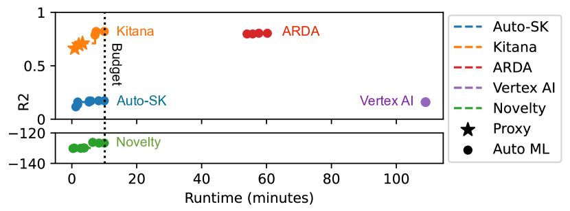
Figure 1 summarizes our major results compared to prior data augmentation techniques (ARDA (Chepurko et al., 2020), Novelty (Li et al., 2021)); AutoML libraries (Auto-sklearn); and cloud AutoML services (Google’s Vertex AI). Since augmentation techniques don’t accept a time budget and return the augmented dataset, we run them to completion and then run Auto-sklearn to derive a model. Both Auto-sklearn and Vertex AI only take the original training dataset as input, thereby neglecting the abundant augmentation opportunities that may be present in the data corpus. We set Auto-sklearn’s budget to 10 minutes and Vertex AI’s budget to 1 hour (minimum allowed), and report $R2$ throughout the model search; Vertex AI doesn’t enforce the budget.

The training set doesn’t have predictive features, so Auto-sklearn and Vertex AI do not find good models. ARDA takes ${\approx}50$ minutes for data augmentation, and the final model is still slightly worse than Kitana ($R2=0.81$ vs $0.82$). Novelty is uncorrelated with model accuracy and degrades the final model. Finally, Kitana’s proxy models (stars) are already highly competitive, and it leaves enough time to train the final model using AutoML (circles).

In addition to higher accuracy, faster results, and cheaper cost, Kitana supports sensible dataset access controls via data release labels. Labels indicate what can be released to the user, and what data providers need to share with Kitana. A data provider can label each dataset so the raw data can be released to the user (RAW), only the trained model can be released (MD), or the user can perform inference using the model but the model cannot be released (API). A user request can specify whether they want the full augmentation plan and associated datasets, a model trained on augmented data, or a prediction API, and Kitana will automatically adjust its search procedure to satisfy data release labels. Although the implementation to support these controls is relatively straightforward, the labels mirror access control expectations in the wild (Lécuyer et al., 2017; Dourish et al., 2004). They also illustrate the complex interaction between dataset access, system design, and user-facing API semantics. We leave a more complete treatment of access control to future work.

We evaluate Kitana using a corpus of 518 datasets collected from open data repositories and compare its performance against existing AutoML services like Auto-Sklearn and Google’s Vertex AI. Across all user requests based on 5 real-world datasets, we find that Kitana is faster, cheaper, and of higher quality than AutoML services. Specifically, Kitana takes less than 1 minute to exceed the accuracy that AutoML reaches after ${\geq}10min$; for the same time budget, Kitana increases the model $R2$ scores by ${\sim}0.05{-}0.30$.

To summarize, we contribute the following:

• The design and implementation of Kitana, an AutoML system that uses practical data augmentation. Kitana efficiently searches a corpus of datasets for augmentation opportunities that increase the final model as compared to using AutoML services alone.

• Kitana leverages careful pre-computation and factorized learning to evaluate each augmentation within ${\sim}100ms$.

• Extensive evaluation against two AutoML systems (Google’s Vertex AI (Ver, 2022) and Auto-sklearn) using a corpus of real-world datasets. We show that Kitana is cheaper and better: Kitana reduces request latency by over $10\times$ for the same model accuracy and increases accuracy by over $30\%$ for the same time budget.

2. Problem Description

This section introduces our terminology, related AutoML services, and the augmentation search problem definition.

2.1. Preliminaries

Kitana focuses on supervised ML tasks over tables.

Tables and Dataset Corpus. Let $D$ denote a general relational table and the list of attributes $S_{D}=[a_{1},\ldots,a_{m}]$ be its schema. A dataset corpus $\mathcal{D}=\{D_{1},...,D_{n}\}$ is a set of tables. We focus on two forms of augmentation: horizontal augmentation unions two tables $D_{1}\cup D_{2}$ that are schema compatible, and vertical augmentation joins two tables $D_{1}\Join D_{2}$ together to add additional attributes.

Supervised ML. In supervised ML tasks like classification and regression, a model with parameters $\theta$ is trained on a tabular dataset $T$ with features $X\subset S_{T}$ and target $Y\in S_{T}$. The goal is to predict $Y$ for unseen $X,Y$ pairs. Users may specify the model type $M$ or use a meta-search process. Model performance is evaluated using cross-validation (Refaeilzadeh et al., 2009) during training and hyperparameter optimization. The final returned model is evaluated once on a test dataset $V$.

AutoML. Today’s AutoML services input $T$ and $Y$, automatically searching for suitable data transformations and model parameters $\theta$. Some also deploy models and provide inference APIs This allows non-experts in ML to benefit from model training and deployment without worrying about the details. Developers can use open-source packages like Auto-sklearn (Feurer et al., 2020) and FLAML (Wang et al., 2021), and commercial solutions like H2O (h2o, 2022). End users can use cloud-based services like Google Vertex AI (Ver, 2022), Microsoft AutoML (MSa, 2022), Amazon SageMaker (sag, 2022), and Oracle AutoML (ora, 2022).

Model training and search are time-critical as the services use hourly pricing: for instance, as of November 2022, Vertex AI charges $\$21.252$/hr on tabular data, Amazon Sagemaker charges $\$0.115-5.53$/hr, and Microsoft AutoML charges $\$0.073-27.197$/hr. Running AutoML longer increases the search space, enhancing the chances of finding accurate models. Since the search can take a long time, users typically set a time budget $t$.

More data is available than ever before—through public government portals, enterprise data lakes, data marketplaces, logging tools, and IoT devices. This is a huge opportunity to go beyond merely model search  (Sambasivan et al., 2021) for AutoML, and to also vertically and horizontally augment training datasets (Li et al., 2021; Chepurko et al., 2020).

2.2. Data Augmentation for Tabular AutoML

We present use cases to motivate Kitana.

Public Health. Consider a public health analyst working with a Manhattan health dataset, which contains features about the patient’s residence, and aims to predict asthma symptoms (sch, 2023). The AutoML-trained model has low accuracy due to the absence of predictive features and examples. She submits her training dataset to Kitana, which quickly finds neighborhood-level datasets about air quality from NYC Open Data (nyc, 2022), restaurant hygiene from Yelp, and additional asthma symptom records about Brooklyn and the Bronx that a colleague had registered. She approves the use of all three datasets, and her model improves considerably.

Churn Prediction. Sales analysts are trying to use AutoML to model customer churn. The initial datasets only contain customer demographic (age and income) and product features (purchase date and price) collected by their own team, which are not predictive. They submit the task to Kitana, which searches the company’s data warehouse used by teams throughout the company. Kitana finds two datasets that greatly improve model performance: a customer engagement dataset containing website visits, which shows how actively customers interact with the company, and a dataset of local unemployment rates, which reflects customers’ purchasing power. The analysts contact the owners of these datasets to gain direct access, and use them to better identify customers likely to churn.

Figure 2. Overview of Kitana Architecture.

2.3. Problem Definition

Let $\mathcal{D}$ be a corpus of datasets. Each dataset $D{\in}\mathcal{D}$ is assigned an access label $l(D){\in}\{RAW,MD,API\}$ from data providers for access control. The labels are ordered $RAW{<}MD{<}API$: $RAW$ allows access to $D$. $MD$ allows access to models $\theta$ trained over $D$, but not $D$ itself. $API$ disallows access to $\theta$, but allows a prediction API that uses $\theta$.

The user submits a tuple $(t,T,M,R)$, which consists of a time budget $t$, training dataset $T$, an optional model type $M$ ($l$ for linear regression, $\cup$ for all models), and return labels $R{\subseteq}\{RAW,MD,API\}$ that describe what Kitana should return $RAW$ for raw augmentation data with the augmentation plan introduced next, $MD$ for model $\theta$, and $API$ for prediction API. User also has a testing dataset $V$ for evaluation, but it’s only accessible by the user.

We search for a good Augmentation Plan $\mathcal{P}=[A_{1},\cdots,A_{n}]$ that specifies a sequence of horizontal or vertical augmentation $A$: Horizontal augmentation contains augmentation data $D_{A}$ and vertical augmentation additionally contains join key $j_{A}$. $A(I)$ applies augmentation to dataset $I$, where $A(I)=I\cup D_{A}$ for horizontal augmentation and $A(I)=I\Join_{j_{A}}D_{A}$ for vertical augmentation. Applying $\mathcal{P}$ to training set $T$ is defined as $\mathcal{P}(T)=A_{n}(A_{n-1}(\cdots A_{1}(T)))$.

The access label $l(D)$ and the requested return labels $R$ limit the search space to $\sigma_{l(D)\leq min(R)}(\mathcal{D})$. When $min(R){\geq}MD$, only horizontal augmentation is allowed because the user can’t vertically augment new features for prediction using $\theta$. $R$ therefore provides a trade-off between performance and explainability: $R{=}\{API\}$ allow all $\mathcal{D}$, but to inspect raw data and model ($min(R){=}RAW$), the search is over a restricted subset.

Next, we present the formal problem definition:

Problem 1.

Given request $(t,T,M,R)$ and testing dataset $V$ (not available during search), find an augmentation plan $\mathcal{P^{*}}$ that maximizes the testing accuracy:

$$\mathcal{P}^{*}= \quad\operatorname*{argmax}_{\mathcal{P}}acc(\theta,\mathcal{P}(V))$$

$$s.t. \quad\theta=AutoML.train(\mathcal{P}(T)),$$

$$\quad t_{data}+t_{md}\leq t,$$ (time budget constraint)

$$\quad\theta\in M,$$ (model type constraint)

$$\quad\forall D\in\mathcal{P}^{*},l(D)\leq min(R).$$ (access control constraint)

where $t_{data}$ and $t_{md}$ are the times for augmentation search and AutoML model search, respectively.

Hardness. Feature selection is NP-hard (Chen et al., 1997) that can be reduced to finding the optimal augmentation plan, where each feature is a normalized vertical augmentation. In practice, applying AutoML to evaluate every augmentation plan is expensive and not scalable.

3. Kitana Overview

We now present the architecture, how Kitana wraps the problem definition to provide AutoML service, and user request lifecycles.

3.1. Kitana Architecture

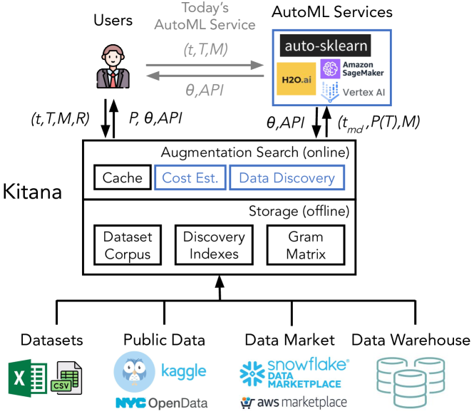
Figure 2 presents the system components and control flow, where the black components are part of Kitana and the blue ones can be outsourced. Section 5 describes the components in greater detail.

Existing AutoML services follow the gray path, where the user submits a request and receives model parameters and/or a prediction API. Kitana, however, acts as an intermediary between users and AutoML. During online operation, Kitana finds the optimal augmentation plan $\mathcal{P}^{*}$ (1), passes the augmented dataset to AutoML. Depending on the request’s return labels, Kitana returns the trained model $\theta$, prediction API, and/or augmentation plan $\mathcal{P}^{*}$.

To search for $\mathcal{P}^{*}$ efficiently, Kitana uses the bottom-up feature selection (Guyon and Elisseeff, 2003) to greedily adds the next best augmentation. It employs proxy models for evaluation to avoid retraining. Then, if the desired model is linear $M=l$, Kitana returns the proxy model. Otherwise, it materializes and sends the augmented dataset to AutoML. During offline setup, data providers register datasets, and Kitana builds sketches and indexes to speed up augmentation search.

Offline Phase. Data providers call Kitana’s $upload(D,l)$ function to upload dataset $D$ with access level $l$ (Section 2.3). Kitana then computes sketches for data discovery and augmentation search—it pre-aggregates attribute profiles for data discovery systems (Kitana uses Aurum (Fernandez et al., 2018a), see Section 5.1.2) and factorized sketches to accelerate augmentation candidate assessment (Section 4). Kitana also applies simple cleaning, standardization, and feature transformations. Optionally, the data provider could upload the profiles and sketches, so Kitana does not have access to the raw datasets.

Online Phase. The user submits request $(t,T,M,R)$, and the Augmentation Search component first checks the cached augmentation plan $\mathcal{P}^{\prime}$ from prior requests with the same training schema $S_{T}$. It then uses data discovery (Aurum (Fernandez et al., 2018a) in our implementation) to find augmentable (union- or join-compatible) datasets; Aurum takes attribute profiles of training data $T$ as input (e.g., MinHash, covariance matrix), and returns a set of candidate augmentations. After that, Kitana evaluates each augmentation candidate via the proxy model and greedily builds the augmentation plan. Kitana further combines proxy model and factorized learning with pre-processing to reduce the evaluation cost to ${\sim}100ms$ per dataset (Section 4).

Kitana needs to judiciously use the time budget, especially if there are no good augmentations. To do so, Kitana uses the sketches to compute the output size of an augmentation candidate. It uses the size to estimate the time to run AutoML $t_{md}$ on the augmented dataset using existing estimation techniques (Popescu et al., 2013; Wang and Khan, 2015; sci, 2022). If the augmentation candidate does not improve the proxy model’s cross-validation accuracy, or when the estimated AutoML cost exceeds the remaining budget (Section 5.2), Kitana materializes the augmented training dataset $T^{\prime}=\mathcal{P}^{*}(T)$ and calls the AutoML service.

Finally, based on user-requested return types $R$, Kitana returns the augmentation plan $\mathcal{P}^{*}$ along with raw augmentation datasets $D$, model $\theta$, and/or the prediction API. The API takes non-augmented records $T^{\prime}$ as input, applies $\mathcal{P}^{*}(T^{\prime})$, makes a prediction using $\theta$, and returns the prediction to the user.

3.2. Request Processing Flow

Algorithm 1 HandleRequest($t,T,M,R$)

1:$\mathcal{P^{*}}=$ initEmptyPlan() $\triangleright$ Empty augmentation plan

2:$\mathcal{P^{\prime}}=$ cacheLookup(T)

3:$\mathcal{P^{*}}=\mathcal{P^{\prime}}$ If $\mathcal{P^{\prime}}$ increases accuracy $\geq\delta$

4:while true do $\triangleright$ Greedily add augmentations

5:     $(acc^{*},A^{*})=(-\infty,\emptyset)$ $\triangleright$ Best accuracy, augmentation found

6:     $\mathcal{A}$= dataDiscovery($\mathcal{P^{*}}(T).profile,R$)

7:     for $A\in\mathcal{A}$  do

8:         $type,D,j=A$ $\triangleright$ Aug. type, data, (opt.) join key

9:         continue If type $=$ “horiz” $\land$ $\mathcal{P^{*}}$ has vert. aug

10:         $\mathcal{P}^{\prime}=\mathcal{P^{*}}.add(A)$ $\triangleright$ Add augmentation to the plan.

11:         $T^{\prime}=\mathcal{P}^{\prime}(T)$ $\triangleright$ Augment data (not materialized).

12:         continue If $M\neq l\wedge t_{remain}<cost(T^{\prime},M)$

13:         $acc,\theta=model.trainAndEvaluate(T^{\prime})$

14:         $(acc^{*},\theta^{*},A^{*},\mathcal{P^{*}}^{\prime})=(acc,\theta,A,\mathcal{P}^{\prime})$ If $acc>acc^{*}$      

15:     break If $\Delta acc^{*}<\delta\vee(M\neq l\wedge t_{remain}<cost(\mathcal{P^{*}}^{\prime}(T),M))$

16:     $\mathcal{P^{*}}=\mathcal{P^{*}}^{\prime}$

17:$\theta^{*}=$ AutoML($t_{remain},\mathcal{P^{*}}(T).materialize(),M$) If $M\neq l$

18:SaveToCache(T, $\mathcal{P^{*}}$)

19:return $\mathcal{P^{*}}$ If$RAW{\in}R$; $\theta^{*}$ If$MD{\in}R$; $buildAPI(\theta^{*},\mathcal{P^{*}})$ If$API{\in}R$

Algorithm 1 outlines the core logic in Kitana when handling a request. The user sends a request $(t,T,M,R)$ and Kitana outputs $API,\theta,\mathcal{P}$ based on user-requested returned types $R$ (Section 2.3).

To start, Kitana initializes an empty augmentation plan $\mathcal{P}$. If $T$ is schema compatible with a prior request, Kitana evaluates the cached plans $\mathcal{P}^{\prime}$ and chooses a plan that most improves the proxy model performance by $\geq\delta$ (L2,3). Kitana then greedily builds the augmentation plan until the estimated time to materialize and train the model exceeds the remaining time budget (L4-16).

In each iteration (L4), Kitana uses data discovery to find a set $\mathcal{A}$ of horizontal and vertical augmentation candidates that are also compatible with the request’s return types and the datasets’ data release labels (L6). Each augmentation candidate $A$ specifies the augmentation $type$ (“horiz” or “vert”), the annotated relation $D$ (Section 4.1), and join key $j$ for vertical augmentations (L8). To simplify the search procedure, Kitana applies horizontal before vertical augmentation (L9). The intuition is that vertical augmentations done before horizontal ones can also occur after, but the reverse isn’t always true because vertical augmentation alters the schema, thus affecting the unionability. Occasionally, applying vertical augmentation first might yield better results. For instance, when the vertically augmented feature matches one feature in horizontal augmentation, and that in horizontal augmentation has a higher quality. Nonetheless, such instances are uncommon, and we did not observe them in experiments. Algorithm 1 can be adapted to explore both horizontal and vertical augmentation by removing L9.

Before evaluating candidate $A$, Kitana adds it to the current plan $\mathcal{P^{*}}$(L10) and cheaply estimates the shape (# of attributes and rows) of augmented training data (L11) by an optimized count query (Section 4.1). If AutoML is needed ($M\neq l$), Kitana uses a cost model to estimate how long AutoML would take on it—if the estimate exceeds the remaining time budget $t_{remain}$, Kitana skips the candidate (L12). In addition, a separate timer thread terminates the augmentation search if the estimated time to run AutoML on the best augmentation plan so far may exceed the remaining budget.

To evaluate candidate $A$, Kitana trains the proxy model and evaluates the model using 10-fold cross-validation (L13). Internally, these two steps are factorized: $T^{\prime}$ in L11 is not materialized and only the aggregates needed for training and evaluation in L13 are computed. Our pre-processing optimization further accelerates this evaluation (Section 4.2), and Kitana keeps the candidate if it improves the best accuracy so far (L14). After evaluating the candidate plan, Kitana keeps it if the accuracy improvement is $\geq\delta$ (L14) and there is time to train the augmented dataset $\mathcal{P^{*}}(T)$ using AutoML (L15). Otherwise, it breaks the loop.

If the user requests models other than linear regression, Kitana materializes the final augmented training dataset $\mathcal{P^{*}}(T)$ and sends it along with the remaining budget $t_{remain}$ and model types $M$ to the AutoML (L17). Otherwise, Kitana skips this step and uses the proxy model. Kitana uses the final model parameters (from AutoML or proxy model) to build an API that first applies $\mathcal{P^{*}}$ then the model for prediction (Section 5.2.4); if AutoML returns APIs, Kitana can wrap them as well, however the user will incur the AutoML service’s costs for inference. Kitana then caches the new plan (L18). Finally, depending on $R$, Kitana returns the augmentation plan (along with the raw datasets), trained model $\theta$, and/or new prediction API (L19).

4. Factorized Data Augmentation

Factorized learning (Khamis et al., 2018; Schleich et al., 2019; Huang and Wu, 2022) trains ML models over the output of a join query $\mathbf{X}=\mathbf{R}_{1}\Join...\Join\mathbf{R}_{k}$ without materializing the join. It treats training as an aggregation function and distributes the aggregation through the joins. As such, the cost is linear in the relation sizes rather than the join results. Factorized learning has been extended to many models, including linear regression (Schleich et al., 2016), ridge regression with regularization, factorization machines (Schleich et al., 2019), classification models using ridge regression (Peng and Cheng, 2020), generalized linear models (Huggins et al., 2017), K-means (Curtin et al., 2020), and SVMs (Khamis et al., 2020).

Our primary contribution is to show that factorized learning is a natural fit for data augmentation. Evaluating an augmentation candidate—materializing the augmented dataset, retraining the model, and cross-validation—is by far the biggest bottleneck (Chepurko et al., 2020; Li et al., 2021) in Kitana, and factorization avoids materialization altogether. Thus, Kitana trains and cross-validates a factorized model as the proxy to evaluate an augmentation candidate, and uses linear regression by default. In fact, proxy models are often more accurate than AutoML models on the user’s original training data (without augmentation), take orders of magnitude less time, and are often preferred in practice for interpretability and reliability reasons (Xin et al., 2021).

However, naively using factorized learning still needs to repeatedly compute these “training” aggregates for each augmentation candidate. Instead, Kitana identifies aggregates sharable across augmentations and pre-computes them—they are computed independently for each dataset in the repository, and in theory could be offloaded to the data provider during dataset registration. This lets Kitana outperform naive factorized learning by over two orders of magnitude on augmentation benchmarks. The rest of this section first introduces the basic concepts in factorized learning, then describes the working sharing opportunities Kitana exploits for efficient data augmentation search.

4.1. Basic Concepts

We now present semi-ring annotations and aggregation push-down, which encapsulate the core factorized learning optimizations. We then illustrate these concepts using linear regression as an example.

4.1.1. Semi-ring Annotations

A semi-ring is a set $\mathbf{S}$ that contains 0 and 1 elements, and supports the binary operators $+$ and $\times$; it is typically defined as the tuple $(\mathbf{S},0,1,+,\times)$. Different semi-rings are designed to support different model types. Each tuple is annotated with an element from $\mathbf{S}$, and $R[t]\in\mathbf{S}$ denotes tuple $t$’s annotation in relation $R$. Relational operators are extended to compute their output relation’s annotations: $\Join$ multiplies the annotations of matching input tuples, while $\gamma$ sums the annotations in the same group-by bin. Formally, given relations $R,T$ with schemas $S_{R},S_{T}$:

(1) $$(R\Join T)[t]= R[\pi_{S_{R}}(t)]\times T[\pi_{S_{T}}(t)]$$

(2) $$(\gamma_{\mathbf{A}}R)[t]= \sum\{R[t_{1}]|t_{1}\in R,t=\pi_{\mathbf{A}}(t_{1})\}$$

Here, $t$ is the output tuple, and $R[\pi_{S_{R}}(t)]$ is the input annotation of $t$ projected onto $R$.

(a) $\mathbf{R}_{1}$

(b) $\mathbf{R}_{2}$

(c) $\mathbf{R}_{3}$

(d) $\mathbf{R}_{1}\cup\mathbf{R}_{2}$

(e) $\gamma(\mathbf{R}_{1})$

(f) $\gamma(\mathbf{R}_{2})$

(g) $\gamma_{A}(\mathbf{R}_{1})$

(h) $\gamma_{A}(\mathbf{R}_{2})$

(i) $\gamma_{A}(\mathbf{R}_{3})$

(j) $\gamma(\mathbf{R}_{1}\cup\mathbf{R}_{2})$

(k) $\gamma((\mathbf{R}_{1}\cup\mathbf{R}_{2})\mathrel{\rule[0.38751pt]{2.70003pt}{0.4pt}\hbox to0.0pt{\hss\rule[5.42494pt]{2.70003pt}{0.4pt}}\mkern-6.5mu\Join}_{A}\mathbf{R}_{3})$

Figure 3. Factorized Learning Example

Example 1.

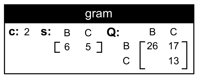
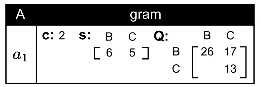
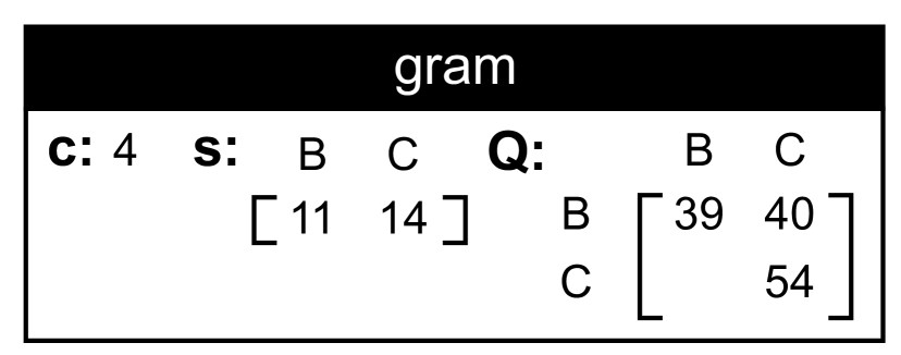
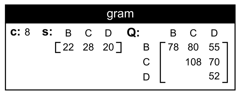
Consider aggregation query $\gamma_{A,SUM(B)}(R_{1}\Join R_{3})$ (Figure 3(a) and Figure 3(c)). To support $SUM(B)$ aggregation, we use natural number semi-ring, and initially annotate $R_{1}[t]=\pi_{B}(t),R_{3}[t]=1$. $R_{1}\Join R_{3}$ will produce a cartesian product (as $A$ has the same value) of four tuples with annotations $2\times 1,3\times 1,2\times 1,3\times 1$. $\gamma_{A,SUM(B)}$ then sums the annotations: for the only $a_{1}$ group, the sum is $2+3+2+3=10$.

The core factorized learning optimization is to push aggregation through joins by exploiting the fact that join distributes over addition as in elementary algebra. For the previous example, we can rewrite $\gamma_{A,SUM(B)}(R_{1}\Join R_{3})=(\gamma_{A,SUM(B)}(R_{1}))\Join_{A}(\gamma_{A,SUM(B)}(R_{3}))$; the sum for group $a_{1}$ then is computed as $(2+3)\times(1+1)=10$. More generally, assuming $j$ is the set of join keys between $R$ and $T$:

$$\gamma_{\mathbf{A}}\left(R\Join_{j}T\right)=\gamma_{\mathbf{A}}\left(\gamma_{\mathbf{A},j}(R)\Join_{j}\gamma_{\mathbf{A},j}(T)\right)$$

This reduces intermediate sizes and thus join-aggregation costs.

4.1.2. Factorized Learning

We now illustrate how linear regression can be expressed as a single semi-ring join-aggregation query.

Linear regression uses training data $\mathbf{X}$ and target variable $Y$ to learn parameters $\theta$ that minimize the model’s squared loss: $\hat{\theta}=arg\,min_{\theta}||Y-\mathbf{X}\theta||^{2}$. The closed form solution is $\theta=(\mathbf{X}^{T}\mathbf{X})^{-1}\mathbf{X}^{T}Y$. By treating $Y$ as a special feature, we can see that the bottleneck computation is the gram matrix $\mathbf{X}^{T}\mathbf{X}$, where each cell is the sum of products between pairs of features. $\mathbf{X}^{T}\mathbf{X}$ has shape $m\times m$, where $m$ is the number of features and is assumed to be much smaller than the number of rows. As a result, computing $\theta$ could be considered as a cheap postprocessing over the small $\mathbf{X}^{T}\mathbf{X}$.

The gram matrix semi-ring (Schleich et al., 2016) helps efficiently compute $\mathbf{X}^{T}\mathbf{X}$. For a training set with $m$ features, the gram matrix annotation is a triple $(c,\mathbf{s},\mathbf{Q})\in(\mathbb{Z},\mathbb{R}^{m},\mathbb{R}^{m\times m})$ that respectively contain the tuple count, sum of features, and sum of products between each pair of features. The zero and one elements are $\mathbf{0}=(0,\mathbf{0}^{m},\mathbf{0}^{m\times m})$ and $\mathbf{1}=(1,\mathbf{0}^{m},\mathbf{0}^{m\times m})$. The $+$ and $\times$ operators between two annotations $a=(c_{a},\mathbf{s}_{a},\mathbf{Q}_{a})$ and $b=(c_{b},\mathbf{s}_{b},\mathbf{Q}_{b})$ are defined as:

(3) $$a+b= (c_{a}+c_{b},\mathbf{s}_{a}+\mathbf{s}_{b},\mathbf{Q}_{a}+\mathbf{Q}_{b})$$

(4) $$a\times b= (c_{a}c_{b},c_{b}\mathbf{s}_{a}+c_{a}\mathbf{s}_{b},c_{b}\mathbf{Q}_{a}+c_{a}\mathbf{Q}_{b}+\mathbf{s}_{a}\mathbf{s}_{b}^{T}+\mathbf{s}_{b}\mathbf{s}_{a}^{T})$$

All rules for combining annotations remain the same.

Finally, computing $\mathbf{X}^{T}\mathbf{X}$ is reduced to executing a single join-aggregation query $\gamma(\mathbf{R}_{1}\Join...\Join\mathbf{R}_{k})$, where aggregation can be pushed down before join as discussed before.

4.1.3. Factorized Model Evaluation

Given the model parameters $\theta$, the semi-ring annotations of the validation table also help accelerate cross-validation. Suppose the evaluation metric is the squared loss: $\sum(y-\theta x)^{2}=\sum(y^{2}-2\theta xy+\theta^{2}x^{2})=\sum y^{2}-2\theta\sum xy+\theta^{2}\sum x^{2}$. This expression decomposes into the sums of pairwise products, which are readily available in the gram matrix semi-ring annotations.

4.2. Factorized Data Augmentation

Although factorized learning quickly trains a single model in one query, augmentation search still needs to execute $O(KU(N+M))$ training queries, where there are $U$ user requests, each final augmentation plan contains $K$ augmentations, and the data discovery service respectively returns $M$ and $N$ horizontal and vertical augmentation candidates. For instance, for an AutoML service with $U=1000$ user requests over $M+N=500$ augmentation candidates and $K=3$ average augmentations per plan, the total number of training queries to execute is around $1000\cdot 3\cdot 500=1.5$ million. Kitana borrows ideas from factorized IVM (Nikolic and Olteanu, 2018) and view materialization for factorized queries (Huang and Wu, 2022) to aggressively pre-compute and share aggregates between these queries. Since each search iteration evaluates every horizontal and vertical candidate, we will first describe optimizations for individual augmentations, and then describe sharing across iterations.

4.2.1. Horizontal Augmentation

Given the current augmentation plan $\mathcal{P}$, horizontal augmentation $Q_{k}^{h}$ will union the plan with the candidate dataset $D_{k}^{h}$. We can use IVM to push the aggregation through union (Nikolic and Olteanu, 2018).

$$Q_{k}^{h}=\gamma(\mathcal{P}(T)\cup D_{k}^{h})={\color[rgb]{0.01,0.40,.8}\definecolor[named]{pgfstrokecolor}{rgb}{0.01,0.40,.8}\gamma(\mathcal{P}(T))}\cup{\color[rgb]{1,0,0}\definecolor[named]{pgfstrokecolor}{rgb}{1,0,0}\gamma(D_{k}^{h})}$$

Example 2.

Suppose we union $\mathbf{R}_{1}$ and $\mathbf{R}_{2}$ (Figure 3(a,b)). The gram matrix of the union is defined as $\gamma(\mathbf{R}_{1}\cup\mathbf{R}_{2})$ (Figure 3(j)), which is equivalent to $\gamma(\mathbf{R}_{1})\cup\gamma(\mathbf{R}_{2})$ (Figure 3(e,f)).

To fit the linear regression model using the gram matrix (Figure 3(j)), we treat B as feature and C as the target variable. $\theta=[\theta_{B},\theta_{0}]$ is then:

$$\theta=(\mathbf{X}^{T}\mathbf{X})^{-1}\mathbf{X}^{T}Y=\begin{bmatrix}\sum B^{2}&\sum B\\ \sum B&\sum 1\end{bmatrix}^{-1}\begin{bmatrix}\sum BC\\ \sum C\end{bmatrix}=\begin{bmatrix}39&11\\ 11&4\end{bmatrix}^{-1}\begin{bmatrix}40\\ 14\end{bmatrix}$$

The key optimization is to pre-compute $\gamma(\mathcal{P}(T))$ at the start of the search iteration, and $\gamma(D_{k}^{h})$ when data providers upload the dataset. $\gamma(\mathcal{P}(T))$ is shared across all $M$ candidate horizontal augmentations, and $\gamma(D_{k}^{h})$ is shared across $U$ user requests where $D_{k}$ is a horizontal candidate. Now, horizontal augmentation simply adds the pre-computed aggregates in near-constant time.

4.2.2. Vertical Augmentation

Vertical augmentation is more complex than horizontal augmentation because pushing aggregation through the join needs to take the join key $j$ into account (so the join can be evaluated). Consider $Q^{v}_{k}$, which augments the current augmentation plan $\mathcal{P}$ with $D_{k}^{V}$ using join key $j$:

$$Q^{v}_{k}=\gamma(\mathcal{P}(T)\mathrel{\rule[0.43057pt]{3.00003pt}{0.4pt}\hbox to0.0pt{\hss\rule[6.02773pt]{3.00003pt}{0.4pt}}\mkern-6.5mu\Join}_{j}D^{v}_{k})=\gamma({\color[rgb]{0.01,0.40,.8}\definecolor[named]{pgfstrokecolor}{rgb}{0.01,0.40,.8}\gamma_{j}(\mathcal{P}(T))}\mathrel{\rule[0.43057pt]{3.00003pt}{0.4pt}\hbox to0.0pt{\hss\rule[6.02773pt]{3.00003pt}{0.4pt}}\mkern-6.5mu\Join}_{j}{\color[rgb]{1,0,0}\definecolor[named]{pgfstrokecolor}{rgb}{1,0,0}\gamma_{j}(D^{v}_{k})})$$

Example 3.

Suppose we have already horizontally augmented $\mathbf{R}_{1}$ with $\mathbf{R}_{2}$, and want to assess the vertical augmentation $(\mathbf{R}_{3},A)$. To do so, we want to compute $\gamma((\mathbf{R}_{1}\cup\mathbf{R}_{2})\mathrel{\rule[0.43057pt]{3.00003pt}{0.4pt}\hbox to0.0pt{\hss\rule[6.02773pt]{3.00003pt}{0.4pt}}\mkern-6.5mu\Join}_{A}\mathbf{R}_{3})$ (Figure 3(k)). We can push down the aggregation to derive $\gamma\left((\gamma_{A}(\mathbf{R}_{1})\cup\gamma_{A}(\mathbf{R}_{2}))\mathrel{\rule[0.43057pt]{3.00003pt}{0.4pt}\hbox to0.0pt{\hss\rule[6.02773pt]{3.00003pt}{0.4pt}}\mkern-6.5mu\Join}_{A}\gamma_{A}(\mathbf{R}_{3})\right)$ (Figure 3(g,h,i)).

$\gamma_{j}(\mathcal{P}(T))$ is shared among all $N$ vertical augmentation candidates with join key $j$. Thus, Kitana pre-computes $\gamma_{j^{\prime}}(\mathcal{P}(T))$ for all of its valid join keys $j^{\prime}$. Kitana also pre-computes ${\color[rgb]{1,0,0}\definecolor[named]{pgfstrokecolor}{rgb}{1,0,0}\gamma_{j^{\prime}}(D^{v}_{k})}$ for all of its valid join keys, and shares them across all $U$ requests where $D^{v}_{k}$ is a vertical candidate. Vertical augmentation is now independent of the dataset size and bound by the cardinality of $j$ (typically small).

4.2.3. Sharing Between Augmentation Plans

Once Kitana finds the best vertical augmentation $(D^{*},j^{*})$ at the end of a search iteration, the next plan is defined as $\mathcal{P}^{\prime}(T)=\mathcal{P}(T)\mathrel{\rule[0.43057pt]{3.00003pt}{0.4pt}\hbox to0.0pt{\hss\rule[6.02773pt]{3.00003pt}{0.4pt}}\mkern-6.5mu\Join}_{j^{*}}\gamma_{j^{*}}(D^{*})$. At the start of the next iteration, Kitana will pre-compute aggregations $\gamma_{j}(\mathcal{P}^{\prime}(T))$ for all valid join keys $j$. Pre-computing $\gamma_{j}(\mathcal{P}^{\prime}(T))$ can re-use aggregations from previous plans. We illustrate this re-use opportunity using a special case where $j\in S_{D^{*}}\wedge j\notin S_{\mathcal{P}(T)}$:

$$\gamma_{j}(\mathcal{P}^{\prime}(T))=\gamma_{j}(\mathcal{P}(T)\mathrel{\rule[0.43057pt]{3.00003pt}{0.4pt}\hbox to0.0pt{\hss\rule[6.02773pt]{3.00003pt}{0.4pt}}\mkern-6.5mu\Join}_{j^{*}}D^{*})=\gamma_{j}({\color[rgb]{1,0,0}\definecolor[named]{pgfstrokecolor}{rgb}{1,0,0}\gamma_{j^{*}}(\mathcal{P}(T))}\mathrel{\rule[0.43057pt]{3.00003pt}{0.4pt}\hbox to0.0pt{\hss\rule[6.02773pt]{3.00003pt}{0.4pt}}\mkern-6.5mu\Join}_{j^{*}}\gamma_{j^{*},j}(D^{*}))$$

Here, ${\color[rgb]{1,0,0}\definecolor[named]{pgfstrokecolor}{rgb}{1,0,0}\gamma_{j^{*}}(\mathcal{P}_{i,j}(T_{i}))}$ has already been computed in a previous search iteration. In general, Kitana aggressively pushes aggregations through joins which reduces the join cost and canonicalizes the plans; it then finds subsets of the query plan that is identical to subsets from a previous iteration (as in the example) and re-uses them.

4.3. Factorized Augmentation Benchmarks

Does pre-computation help, or simply add additional overhead? We now benchmark horizontal and vertical augmentation to evaluate our pre-computation optimizations (Kitana) against naive factorized learning (Factorized). Specifically, we evaluate 1) what factors influence the performance of Kitana? and 2) what are the costs of offline pre-computation?

Dataset. We generate a synthetic dataset $T[f_{1},f_{2},f_{3},Y,j]$ with three features, a $Y$ variable, and a join key with a default domain size of $30$. The feature and $Y$ values are randomly generated. $|T|=1M$ tuples by default. We will horizontally and vertically augment $T$.

4.3.1. Horizontal Augmentation Performance.

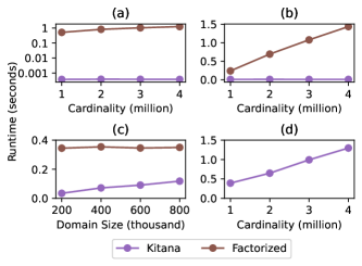
We create augmentation dataset $D^{h}$ using the above procedure, vary $|D^{h}|\in[1M,4M]$ tuples, and measure the runtime to compute $\gamma(T\cup D^{h})$. Figure 4(a) shows that Kitana is ${>}3$ orders of magnitude faster than Factorized. At $|D^{h}|=4M$, Factorized takes ${\sim}1.2s$ while Kitana takes ${\sim}400{\mu}s$. Factorized grows linearly in relation cardinality as it needs to compute the aggregates online, while Kitana is constant.

Figure 4. Factorized Augmentation Benchmarks. (a) Horizontal Augmentation Runtime (log) when varying augmentation dataset cardinality. (b) Vertical Augmentation Runtime when varying user dataset cardinality. (c) Vertical Augmentation Runtime when varying join key domain size. (d) Offline Pre-computation Runtime when varying the cardinality.

Figure 5. Factorized Augmentation Compared to models from previous works. Fac is factorized learning without pre-computations. (a) Horizontal Augmentation Runtime. (b) Vertical Augmentation Runtime.

4.3.2. Vertical Augmentation Performance.

We create augmentation dataset $D^{v}[j,f]$ containing the join key $j$ and one feature $f$. The performance of Kitana is bounded by the join key domain size and is independent of the cardinality of the query dataset. Figure 4(b) varies $|D^{v}|\in[1M,4M]$ but fixes $|j|=30$, and we see that Kitana is constant while Factorized grows linearly. Figure 4(c) fixes $|D^{v}|=1M$ but varies $|j|\in[200k,400k,600k,800k]$. Kitana grows linearly because the aggregates are larger. However, Kitana still avoids recomputing aggregates from scratch, and is ultimately upper-bounded by Factorized.

4.3.3. Sharing Between Augmentation Plans.

We create three datasets $R_{1}[A,B,Y],R_{2}[B,C,f_{1}],R_{3}[C,D,f_{2}]$ with two features, a $Y$ variable, four join keys $A,B,C,D$ with domain size $200k$, and each with $1M$ tuples. We consider original plan $\mathcal{P}=R_{1}\Join_{B}R_{2}$ and new plan $\mathcal{P}^{\prime}=R_{1}\Join_{B}R_{2}\Join_{C}R_{3}$. The task is to compute $\gamma_{j}(\mathcal{P}^{\prime})$ for $j\in\{A,B,C,D\}$. Without pre-computation, the four aggregates take $3.13s$ to complete. With aggregates of original plan $\gamma_{j}(\mathcal{P})$ for $j\in\{A,B,C\}$ pre-computed and re-used, we can compute the aggregates for $\mathcal{P}^{\prime}$ in $1.75s$, thus $1.8\times$ speedup.

4.3.4. Offline Pre-computation Overhead

Kitana’s pre-computation essentially shifts the cost for Factorized to offline rather than during augmentation search. Figure 4(d) reports pre-computation time while varying $|D^{v}|\in[1M,4M]$. It grows linearly with $|D^{v}|$, but is only ${\sim}1.3s$ for $4M$ tuples. This is because the gram-matrix semi-ring decomposes into sum-aggregation operations that are optimized in analytical DBMSes and data science libraries like numpy (Harris et al., 2020). Finally, notice that pre-computation is run once per dataset, and can be delegated to the data provider by extending $\textsf{Kitana}.upload(D,l)$.

4.3.5. Comparison against Other Models.

Although Kitana improves considerably over naive factorized learning, prior data augmentation works don’t apply factorized learning and are even slower. To highlight the performance disparities, we now compare Kitana, factorized learning (Fac), and prior augmentation techniques.

We consider previous models for both horizontal and vertical augmentations. For horizontal augmentations, Li et al. (Li et al., 2021) computes novelty by training a 3-NN regressor (KNN) for each augmentation candidate. We test the training time on a horizontal augmentation candidate with $|D^{h}|=1M$. Figure 5(a) shows that Kitana is four orders of magnitude faster. For vertical augmentation, ARDA (Chepurko et al., 2020) joins all tables at once, injects random control features, and trains a random forest to perform feature selection. We generate $|D^{v}|$ following Section 4.3.2 (without feature injection), and limit ARDA’s random forest to a max depth of 3 and 0.1 sampling rate. Figure 5(b) shows that Kitana is three orders of magnitude faster.

In conclusion, prior works incur unacceptably high search costs that will consume the user’s budget. Kitana uses factorized learning and prudent pre-computation to accelerate augmentation search by 2-4 orders of magnitude, at a level that makes data augmentation search for AutoML realistic.

5. Kitana Design and Implementation

This section describes each component in Kitana’s architecture (Figure 2). We will present the offline and then online phases.

5.1. Offline Phase

While offline, Kitana collects a large volume of datasets for augmentations, preprocesses them, and builds the necessary indexes to serve requests efficiently during the online phase.

5.1.1. Data Collection.

Enterprise users can make the best of datasets already in the data warehouses by uploading them to Kitana with different access labels. They can also upload additional datasets bought from data markets (aws, 2022; sno, 2022), or use existing web crawlers (Kausar et al., 2013) to collect public dataset (nyc, 2022; cms, 2022; dat, 2022) with $RAW$ access labels.

5.1.2. Data Preprocessing

Kitana preprocesses data corpus offline for efficient online Data Discovery and Factorized Learning.

Feature Engineering. Kitana performs standard feature engineering (Kuhn and Johnson, 2019), including missing values imputation, feature transformations (e.g., PCA, polynomial, and interaction features) and standardization (center and re-scale numeric attributes). We note that Kitana is robust against inadequate missing value imputations because it uses ML performance as the criteria for search. For instance, if vertical augmentation leads to numerous missing values that are hard to impute, the resulting model performance is likely to be compromised, prompting Kitana to forgo the augmentation. More advanced feature engineering and imputation methods can turn a “poor” augmentation into a “good” one; we defer the investigation of more advanced methods to future work.

Data Discovery. Data discovery finds augmentation candidates for a given table. It does so by computing a profile (e.g., minhash and other statistics) for each table and building an index over them. Kitana uses Aurum (Fernandez et al., 2018a) by default, which builds a discovery index offline. The index finds union-able tables based on syntactic schema matching and value similarity, and join-able tables based on a combination of similarity, containment, and semantic similarity (Fernandez et al., 2018b) metrics. Kitana can use other data discovery systems (Zhang and Ives, 2020; Bogatu et al., 2020; Castelo et al., 2021) as well, and they build similar types of indexes offline.

Gram Matrix. To support efficient online factorized learning, Kitana pre-computes aggregated gram-matrix for each dataset $D$ in the corpus as discussed in Section 4.2; the aggregates include $\gamma(D)$ and $\gamma_{j}(D)$ for each valid join key $j$. Building the gram-matrix has low overhead as shown in Section 4.3, and can potentially be offloaded to the data providers during dataset upload.

Re-weighting. For vertical augmentation, one-to-many join results will have a much larger number of tuples and potentially skew the training data distribution. To avoid this, we re-weigh the semi-ring such that, for each join key value, its semi-ring has a count of 1. Given the aggregated gram-matrix semi-ring $(c,s,Q)$ for each join key, we multiply it with $(1/c,0,0)$ to $(1,s/c,Q/c)$.

5.1.3. Handling Updates

Kitana efficiently supports deletes, inserts, and updates of datasets in the corpus. First, the data discovery system we use supports incremental maintenance (Fernandez et al., 2018a). Second, we use factorized IVM (Nikolic and Olteanu, 2018) to update the semi-rings incrementally.

5.2. Online Phase

During the online phase, Kitana preprocesses the user’s base table and checks the request cache in case it can save computation. Then it triggers the augmentation process described in 3.2, while balancing the budget usage. It uses an AutoML service to find a good model and finally it constructs a response to the user.

5.2.1. Request Preprocessing

Given the user’s training dataset $T$, Kitana computes a profile and uses it to probe the discovery index to find augmentation candidates (L6). By default, Kitana splits $T$ into 10-folds for cross-validation, but optionally accepts a user-provided validation set (e.g., in case of train-test imbalance). At the beginning of each iteration (L4-18), Kitana pre-computes $\gamma(\mathcal{P}(T))$ and $\gamma_{j}(\mathcal{P}(T))$ for all valid join keys to share computations (Section 4.2).

5.2.2. Request Cache

Caching augmentation plans helps when the training data from two requests match the schema (L2). We use the most recent plan that improves the performance by ${\geq}\delta$, where $\delta$ ($0.02$ by default) is also used for early stopping ((L15). We design a two-level Request Cache: each schema stores a list of $K$ plans ($K=1$ in the experiments). The list is ordered and replaced using LRU; a plan is considered used if it improved the model by ${\geq}\delta$.

5.2.3. Cost Model

Kitana shortcuts to AutoML once there is not “enough time” left (L16) predicted by a cost model. The cost model $f(n,m)\to\mathbb{R}^{+}$ maps the shape $n\times m$ of the augmented training dataset $T^{\prime}$ as input, and outputs the time to train user-requested model $K$ times ($K=5$ by default). The function should over-predict to ensure Kitana is not worse than AutoML without augmentation search, and is typically tuned to specific hardware and model types.

Since Kitana uses Auto-sklearn (Feurer et al., 2015) as its default AutoML library, we use scitime (sci, 2022) to construct the cost model. Scitime is an open-sourced project for training time estimation for Sklearn algorithms given training data shape; we found it accurate in our experimental evaluation. Scitime can be customized to other AutoML systems (e.g., FLAML (Wang et al., 2021)) by executing them on randomly generated data of varying sizes, collecting training time, and training a model (defaulting to random forests) to predict training time. ML cost estimation is an active area of research (Popescu et al., 2013; Wang and Khan, 2015), and we expect cost estimators to improve over time.

5.2.4. Prediction API Construction

Kitana constructs and exposes a prediction REST API if the request $R$ includes $API$ in the return labels. The API takes as input a dataset $T^{\prime}$ with the same schema as $T$, and outputs the prediction values for each record. Internally, it applies all vertical augmentations from $\mathcal{P^{*}}$ to $T^{\prime}$, and then uses the final model $\theta$ to perform the predictions. If Kitana internally uses a cloud AutoML service rather than Auto-sklearn, then Kitana will call the service’s own prediction API. Note that this will incur monetary charges that the user is responsible for.

Meet time budget ($10$ minutes)

Exceed time budget

SK

FML

Fac + SK

K + SK

K + FML

ARDA + SK

K + Vertex AI

Data

Task

Size

Score

Score

Score

Score

Score

Score

Time

Cost

Score

Time

Cost

$D_{1}$ (vac, 2022)

R

0.8MB

[0.10,0.10]

[0.11,0.11]

[0.22,0.22]

[0.22,0.22]

[0.22,0.22]

[0.22,0.22]

[23,23]

[0.30,0.30]

[0.22,0.22]

[115,124]

[40.73,40.92]

$D_{2}$ (gen, 2022)

R

4.1MB

[0.17,0.17]

[0.17,0.17]

[0.55,0.55]

[0.82,0.82]

[0.82,0.82]

[0.81,0.82]

[59,61]

[0.77.0.80]

[0.91,0.91]

[116,131]

[41.09,46.4]

$D_{3}$ (nb3, 2022)

R

33MB

[0.45,0.45]

[0.46,0.46]

[0.68,0.68]

[0.74,0.74]

[0.73,0.74]

OOT

[0.70,0.71]

[125,150]

[44.28,53.13]

$D_{4}$ (uk6, 2022)

C

0.7MB

[0.60,0.60]

[0.60,0.60]

[0.71,0.71]

[0.73,0.73]

[0.73,0.73]

[0.72,0.73]

[22,22]

[0.29,0.29]

[0.70,0.70]

[118,127]

[41.80,44.98]

$D_{5}$ (eco, 2022)

C

10MB

[0.77,0.77]

[0.77,0.77]

[0.89,0.89]

[0.91,0.92]

[0.94,0.94]

[0.92,0.92]

[64,66]

[0.83,0.86]

[0.98,0.98]

[117,133]

[41.44,47.11]

$D_{6}$ (y2h, 2023)

C

35MB

[0.85,0.85]

[0.85,0.85]

[0.85,0.85]

[0.87,0.87]

[0.87,0.87]

OOT

[0.87,0.88]

[131,148]

[46.40,52.42]

Table 1. AutoML performance across different baselines. The performance score ($R2$ for regression and accuracy for classification) is measured in 10 runs, and we report the [minimum, maximum]. The baselines are categorized based on whether they meet or exceed the time budget, and the best performance is highlighted in red. The (K+/Fac+) SK and FML are allocated a budget of 10 minutes (cost $0.13). K+Vertex AI’s budget is set to 1 hour (the minimum allowed) but it exceeds the budget. Due to the protracted time taken by ARDA, we extended its budget to 2 hours, though it still runs out of time (OOT) for larger datasets. The final results show that Kitana (K+SK/FML/Vertex AI) outperforms the other baselines with high performance at lower costs.

6. Evaluation

Our evaluation strives to understand three main questions: Q1: Can Kitana improve task performance beyond real-world AutoML services? Q2: How does Kitana adapt to varying budgets and the percentage of useful datasets? Q3: how sensitive is Kitana performance to different components and their configurations?

6.1. Setup

Datasets. We collected 518 datasets from NYC open data (nyc, 2022) (364 datasets, 3.1 GB) and CMS Data (cms, 2022) (154 datasets, 7.4 GB). To create user requests, we adopt a leave-one-out strategy: 1 dataset is chosen for AutoML, and the rest 517 datasets are searched for augmentation. For each requst, the dataset is split into 80% training data and 20% testing data.

AutoML:

• SK: Auto-sklearn (Feurer et al., 2015) is an open-source library that performs hyperparameter optimization over a broad range of ML models including multilayer perceptron, KNN, SVM, tree-based models (decision tree, gradient boosting and random forests).

• FML: FLAML (Wang et al., 2021) is also an open-source AutoML library, but it uses mostly tree-based models.

• Vertex AI (Ver, 2022) is a cloud-based AutoML service by Google. It currently has a minimum time budget of 1 hour and doesn’t enforce the budget. Therefore, we run Vertex AI until completion.

Baselines:

• AutoML-Only directly sends the request to an AutoML service (SK, FML, or Vertex AI) without augmentations.

• Kitana (K) applies our full suite of optimizations to speed up the augmentation search, uses the cost model balances the budget split, and sends the augmented data to AutoML. K uses the cost model in Section 5.2.3 to balance between augmentation and AutoML. For Vertex AI, predicting the cost is challenging. We, therefore, allocate a fixed budget of $5min$ for K, which, while small compared to the ML cost (${>}1hour$), shows sufficient for K to find predictive augmentations in our experiments.

• Factorized (Fac) is similar to Kitana, but doesn’t pre-compute sketches. It computes the aggregates online and fully re-trains factorized proxy models to assess candidate augmentations.

• ARDA (Chepurko et al., 2020) is the SOTA data search algorithm for ML, which joins candidate augmentations (with pre-aggregations to avoid many-to-many joins), injects random features, and trains models (random forests and sparse regression) over the join to assess features. We run ARDA with its default setting (20% random injected features, $10$ rounds of injection, random forests with 3 max depth, 10% sampling rate, and $100$ trees).

Setup. All experiments run in a single thread on a GCP n1-standard-16 VM, running Debian 10, Xeon 2.20GHz CPU, and 60GB RAM. We implemented Kitana in Python 3. To compute monetary costs, we report computation costs because they dwarf storage costs. For instance, Google Cloud storage costs $0.046/GB/month, while running an n1-standard-16 instance costs about $\$388.36$/month.

6.2. Q1: Does Kitana use Data Effectively?

We first evaluate requests using six representative datasets (regression/classification tasks , varying sizes) for detailed insights. Then, we scale up to all 518 datasets via a leave-one-out strategy. All requests are run 10 times.

6.2.1. Exploratory Study

We first conduct an exploratory comparison of Kitana with existing AutoML services and data augmentation search algorithms on price and model performance, and show that Kitana can 1) reach the same or greater model accuracy for considerably lower cost, 2) reach far higher model accuracy for the same cost, and 3) often times reach a higher accuracy at a lower cost.

Setup. We construct requests (regression, classification) using six datasets with varying sizes (${\leq}1MB$, $1{-}10MB$, ${>}10MB$). Model performance measures $R2$ for regression and accuracy for classification. We evaluate Auto-sklearn (SK), FLAML (FML) and Vertex AI (Ver, 2022), with or without data augmentation search (using K, Fac or ARDA). Since SK is not hosted, we evaluate SK and K+/Fac+SK on a GCP n1-standard-16 VM and fix the time budget of $10$min ($\$0.13)$; we find that $10$min is sufficient for model convergence. ARDA exceeds $10$min, and we cap its runtime at $2$ hours. Vertex AI is set to its minimum budget of 1 hour, though it exceeds the requested budget. We report results over 10 runs.

Results. Table 1 summarizes the min/max model performance (Score) from 10 runs, runtime in minutes (Time), and the cost in USD (Cost); we highlight the highest model performance in red. We find that the model performance was consistent across all 10 runs (min/max difference ${\leq}0.01$). SK and FML exhibit similar performance. Vertex AI also has comparable model performance but takes an order of magnitude longer to run, so we did not report it.

Adding data augmentation (K+) improves the model quality by a large margin (e.g., $0.16{\to}0.91$ for $D_{2}$ (gen, 2022)) for most user requests. However, for $D_{6}$(y2h, 2023), there aren’t many augmentations to greatly improve model performance. Overall, Kitana provides an opportunity to balance data augmentation and AutoML. Compared to K, Fac takes longer to find augmentations as it doesn’t pre-compute sketches. This results in less time for dataset search, which explains its lower performance. ARDA is comparable to K but much slower and costlier due to join materialization and expensive model training—ARDA times out for $D_{3}$ and $D_{6}$.

Figure 6 reports the cost for Kitana to achieve the same or higher model quality as SK, FML and Vertex AI (lower right is better). In every case, Kitana is better. For $D_{2}$, Kitana reduces the cost from $\$0.13$ (SK) or $\$38.6$ (Vertex AI) to merely $\$0.01$, while improving the $R2$ from $0.17$ to $0.66$.

Figure 6. Cost for Kitana to reach or exceed the model quality of Auto-sklearn and Vertex AI (shapes) for different user requests (color). Kitana trains higher quality models ${\sim}10\times$ (${>}100\times$) cheaper than AutoSklean (Vertex AI).

Figure 7. Baseline performance (testing R2) over time. $\bigstar$ is for proxy model and $\bullet$ is for AutoML model performance.

6.2.2. In-depth Study

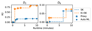
We now study requests $D_{2}$ and $D_{6}$, which respectively showed the most and least improvement from dataset search. $D_{2}$ predicts the ELA test scores across schools in 2013-2016, while $D_{6}$ predicts the ownership type of nursing homes. Since SK incrementally adds models to an ensemble, we are able to report its $R2$ over time. For Kitana, we also report the proxy model in each augmentation search iteration.

Figure 7 plots model performance (y-axis) by runtime (x-axis) for SK with and without K (color). We report the proxy (star) and AutoML (circle) models. For $D_{2}$, Kitana reaches an $R2$ of ${>}0.6$ in less than 1 minute, whereas AutoML-only never exceeds $0.2$ even after 10 minutes. This highlights the importance of high-quality features over pure compute (Sambasivan et al., 2021; Chepurko et al., 2020). Even though $D_{6}$ is $35MB$, Kitana can still find a useful augmentation within a minute because its cost is proportional to the join key’s domain size and not data size (Section 4.3). Kitana quickly switches to AutoML as no more datasets improved the proxy’s $R2$ by $\delta{=}0.02$ (L15).

We found that the datasets in the final augmentation plans were logically relevant to the requests. For $D_{2}$, the sequence of datasets are: school quality report (cbf, 2016) (Student Attendance Rate, Percent of English Language Learners), neighborhood demographic distributions (iuv, 2016), and historical math test scores (b9u, 2012) from 2006-2012. These are all relevant to ELA test scores. Kitana augmented $D_{6}$ with provider information (pro, 2023) (number of beds, quality measure scores), but we could not find other related datasets in our corpus.

6.2.3. Comprehensive Study

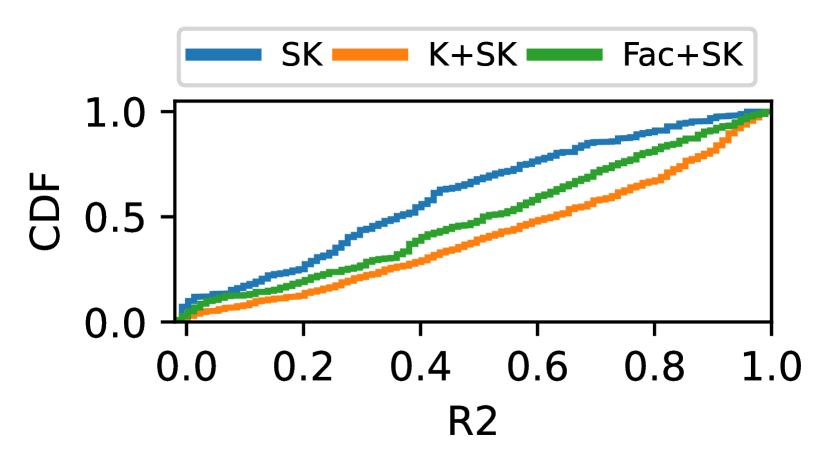
To test the generalizability of our previous findings, we compare SK, K+SK, and Fac+SK using all 518 datasets; for each dataset in the corpus, we remove it from the corpus and use it as the request. We set the time budget to $10$min, and report the median of 10 runs.

Figure 8(a) shows the cumulative density function for model performance (lower curve is better). K+SK and Fac+SK respectively improve the median R2 by $0.25$ and $0.17$ over SK alone. Figure 8(b) displays the heatmap of model performance across SK (x) and K+SK (y). K never degrades model performance (all points are above the diagonal). Although some datasets report low model performance and negligible improvements from dataset search (bottom left corner), there is a long tail of large model improvements (top left corner) of up to $0.85$.

(a) Cumulative distribution function (CDF) of model performance.

(b) Heatmap of the model performance between K+SK and K.

Figure 8. Model performance over 518 datasets using leave-one-out strategy. (a). Both K+SK and K+FML show comparable performance and demonstrate significant improvements over K. Fac falls in the middle, as it requires more time for searching. (b). K+SK outperforms K (above diagonal) on a range of datasets, with a long tail of significant improvements (upper left corner) up to $0.85$.

6.3. Q2: Kitana Adaptability

Our previous experiments used a generous time budget and a corpus that contains good augmentation candidates. We now study how Kitana adapts under varying time budgets, and when there are no good augmentation opportunities.

6.3.1. Varying Budget

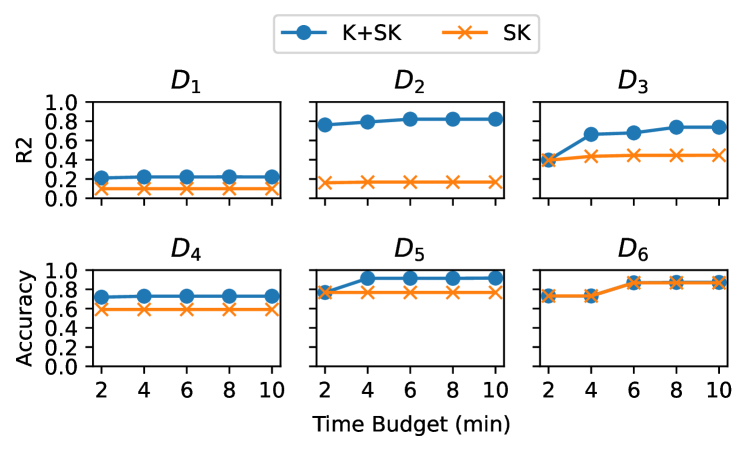
We repeat the experiment from Section 6.2 but vary the time budget of each request to $\{2,4,6,8,10\}$ minutes. We run each request 10 times and report the median performance.

Figure 9(a) shows that Kitana adapts to shorter budgets by finding augmentations that require less AutoML training time. Small datasets (${<}1MB$) require less training time and Kitana improves model quality even when limited to $2$min. For larger datasets, Kitana uses the cost model to allocate enough time for AutoML, and improves over SK considerably when there is enough time to accomodate augmentations. $D_{6}$ is an exception because the corpus does not contain useful augmentations. In all cases, Kitana never performed worse than SK.

(a) Kitana performance when varying time budgets. Kitana adapts to lower budgets by choosing cheaper but effective augmentations.

(b) Kitana performance on synthetic data corpus when varying the number of predictive augmentations. Kitana is able to identify these augmentations and achieve similar performance to the omnious search (upper bound) due to the effectiveness of proxy models.

Figure 9. Kitana adaptability experiments.

6.3.2. Vary Predictive Augmentations.

How does Kitana perform when the predictive augmentations are limited or abundant? Can Kitana effectively identify all the predictive augmentations, compared to an omniscient search engine that knows all predictive augmentations and doesn’t have time constraints? Addressing these is challenging for real-world datasets as the ground truth of predictive augmentations is unknown. To overcome this, we employ synthetic experiments that create predictive augmentations.

Setup. For user request, we create a dataset $R[y,J_{1},...,J_{10}]$ of $1M$ rows, where $J_{i}$ join key of random integers in $[1,10K]$. We create $10$ ground truth feature tables $F_{i}[J_{i},f_{i}]$ of $10K$ rows, where $f_{i}$ are random floats in $[0,1]$. For $y$, we consider either a linear ($y=\sum_{i=1}^{10}f_{i}$) or a non-linear relationship ($y=\sum_{i=1}^{10}f_{i}^{2}$) with the features.

We create both horizontal and vertical augmentations. We introduce a train-testing imbalance, where the test and validation datasets are uniform samples of $10K$ rows from $R$, whereas the training dataset is a non-uniform partition of $R$: we make the first feature $f_{1}$ public, and divide $R$ into $11$ partitions evenly based on $f_{1}$. The first partition is used as training, and the rest are horizontal augmentations. For the vertical augmentation, we create noisy versions of $f_{2},...,f_{9}$ to simulate the real-world corpus: for each feature, we create $10$ predictive augmentations $A_{i}[J_{i},c_{i}]$, where $c_{i}$ varies in correlation with $f_{i}$ (Kaiser and Dickman, 1962). Specifically, the correlation coefficient $\phi$ is drawn from the inverse exponential distribution $\text{min}(1,1/\text{Exp}(10))$, and $c_{i}$ is the weighted average between $f_{i}$ and a random variable, weighted by $\phi$. There are $100$ predictive augmentations in total ($10$ horizontal and $90$ vertical).

We build a data corpus of $100$ datasets, and vary the number of predictive augmentations $\{0,1,5,10,50,100\}$ in them by choosing random samples from the $100$ predictive augmentations; the rest datasets are union-able or join-able relations but populated with random numbers. We run K+SK with a $10$min budget, and an Omniscient search procedure that joins all predictive augmentations and runs AutoML until convergence without time constraint.

Result. Figure 9(b) shows the results. The baseline training data is unbalanced, so the starting points ($R2$) for both are negative. However, with more predictive augmentations, Kitana can find them and achieve near-identical performance to Omniscient search ($R2$ difference $\leq 0.01$), for linear and non-linear relationships.

	Time	Training R2	Testing R2
Kitana	0.01s	0.995	0.994
Novelty	9.72s	0.773	-0.232

Table 2. Model performance for horizontal augmentation.

6.4. Q3: Component Sensitivity

We now evaluate Kitana when restricted to horizontal augmentation only against recent data augmentation work by Li et al. (Li et al., 2021), and also evaluate the effects of request caching across user requests.

6.4.1. Horizontal Augmentation Comparisons

Recent works, such as the Acquisition algorithm by Li et al. (Li et al., 2021), also study the problem of horizontal augmentation. At a high level, given a corpus of datasets, Acquisition seeks sample “novel” records from datasets, based on a custom “Novelty” metric. Novelty is estimated by unioning subsets of the user and augmentation candidates, and fitting a 3-NN classifier to predict which dataset a given record is from. The intuition is that ”novel” data can be more easily classified since it exhibits distinct characteristics.

The key limitation of the novelty measure is that it is oblivious to the actual prediction task, as defined by the test distribution. If the data corpus offers union-compatible data that is irrelevant to the test distribution (common for the data lake in the wild), this data will have high novelty simply if they are dissimilar to the training data. In contrast, Kitana directly evaluates augmentations with respect to the training data through cross-validation, which is expected to be representative of the test data.

Setup. We compare Kitana with a variation that replaces Lines 13-14 in Algorithm 1 to rank augmentation candidates using Novelty. This also means that augmentation search does not benefit from factorized learning. We measure the time to search for the top one horizontal augmentation candidates, and the model accuracy after running AutoML for $2$ minutes over the augmented dataset. Following Li et al. (Li et al., 2021), we use the RoadNet (roa, 2022) mapping dataset (434,874 tuples) with schema (lat, lon, altitude), and partition it along lat and lon into a $8\times 8$ grid. Each partition is a candidate horizontal augmentation. The regression task uses lat, lon to predict altitude, and the user’s training $T$ and testing $V$ datasets are both 0.5% samples from partition 1. In this way, most horizontal augmentations are dissimilar but irrelevant.

Acquisition uses a reinforcement learning framework to estimate a dataset’s novelty because there is a cost to sample from each augmentation candidate. In our case, we directly evaluate the true novelty in order to study the upper bound of their approach.

Results. Table 2 reports that Kitana is orders of magnitude faster than Novelty because the latter trains a classification model for each augmentation but does not benefit from factorized learning. Although both approaches have a high R2 on the training data, Novelty prefers augmentations dissimilar to partition 1, which skews the augmented training data and leads to a low testing R2 score.

6.4.2. Request Cache.

Our experiments so far focused on a single user request, however an AutoML service is expected to serve many requests over time, from the same or different users that perform the same or different tasks. How much does the request take advantage of the similarity between multiple user requests?

Setup. We create a synthetic benchmark consisting of 20 users and 300 candidate vertical augmentations per user, for a total of 6000 augmentation candidates. Each user dataset requires 2 augmentations to train a perfect proxy model (R2=1). To test the case of failed cached augmentation plans, we group the users into 10 pairs and assign each pair a unique schema. Thus, each pair of users ($A$, $B$) will match each other’s cached augmentation plans, but $A$’s plan will not improve $B$’s model and vice versa.

We generate sequences of 50 user requests, where the $i^{th}$ user is drawn from a Zipfian distribution over the 20 users. We vary the parameter $\alpha\in[0,7]$; $0$ is uniform, while $7$ is heavily skewed. To pressure test the request cache, we limit the cache size to accommodate 5 schemas and 1 plan per schema.

(a) Sequence Runtime.

(b) Gender request with cache.

(c) Cache performance (log) zoom in for alpha = 1.

Figure 10. Request Cache Experiment Result. The runtime of a sequence of user requests has been reduced because of the cache. The reduction in run-time can improve final model performance as Kitana has more budgets.

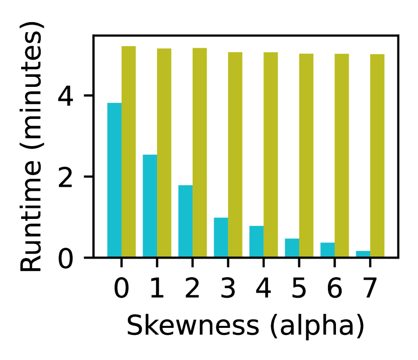
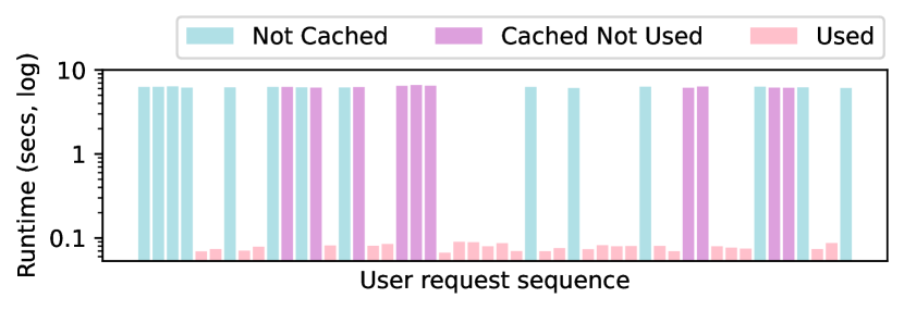
Results. Figure 10(a) reports the runtime for all 50 requests as the Zipfian skew increases. Compared with no caching, the cache reduces the runtime by $26.8\%$ given a uniform distribution ($\alpha=0$) and by $96.7\%$ when the requests are nearly all the same ($\alpha=7$).

Figure 10(c) examines the per-request runtimes when $\alpha=1$. We see that cache hits reduce the request runtime by over $100\times$, and also that evaluating unhelpful cached plans (purple) incurs negligible overhead (${\sim}1\%$) as compared to a cache miss (blue).

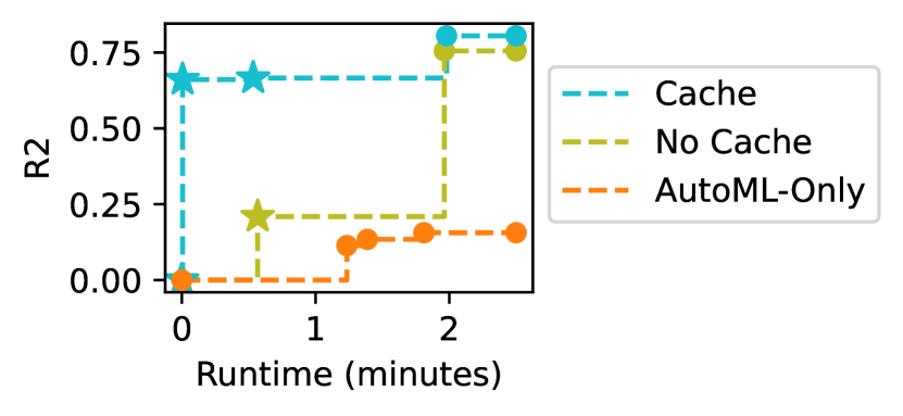
A cache hit both reduces the augmentation search time, and gives AutoML more time to find a better model. To see this, we first cache the augmentation plan generated by the Gender user request from Section 6.3 that has a 5-minute budget. We then generate a similar request with a resampled training dataset and a reduced budget of 2.5 minutes. Figure 10(b) shows that the cached plan immediately increases the proxy model’s quality to an R2 of ${\sim}0.7$. This leads to a better final augmentation plan, and ultimately a higher quality model as compared to a no-cache setting (${\sim}0.75\to{\sim}0.8$).

7. Related Work

We now distinguish Kitana from related work.

AutoML: AutoML services allow non-ML experts to train high-quality models. AutoML is time-critical as it charges hourly (e.g., Vertex AI charges $\$21.252$/hr for tabular datasets). Existing AutoML services (Ver, 2022; sag, 2022; MSa, 2022; h2o, 2022) are model-centric: the training dataset is fixed and all work is focused on transforming the training dataset (e.g., PCA, polynomial, and interaction features) and model search. As a result, the final model is only as good as the quality of the training dataset. Kitana provides an API-compatible interface to existing AutoML, but is data-centric that further searches for new tabular datasets to augment the training data with new features and/or examples. Our experiments show that Kitana is orders of magnitude more cost-effective than existing AutoML alone, and achieve almost the same result when no helpful data augmentation is present.

Model Augmentation: Recent works propose horizontal or vertical augmentation techniques to improve ML models. For instance, Li et al. (Li et al., 2021) focuses on horizontal augmentation. They sample records from a set of relations based on a “Novelty” measure, assuming that record diversity will improve model accuracy, which may not hold for the data lake in the wild. Our experiments show that the model accuracy can decrease after augmentation.

Other works such as ARDA (Chepurko et al., 2020) apply specialized feature selection techniques that require iterative training of complex models (e.g., random forest). These techniques are ill-suitable for time-critical tasks such as AutoML: they take orders of magnitudes more time than Kitana, and even at such high costs, they empirically don’t show better results than Kitana (Figure 1).

Data Discovery: Nowadays data warehouses and data lakes leverage data discovery (Fernandez et al., 2018a) or catalogs (cat, 2022b, a; col, 2022; dat, 2022) systems to find candidate datasets or sellers. Data discovery search interfaces typically take natural language, datasets, or schemas as input. Kitana uses existing data discovery systems (Fernandez et al., 2018a) to identify vertical and horizontal augmentation candidates and is agnostic to the specific discovery mechanism.

Views are commonly used for access control (Rizvi et al., 2004). They prevent access to the underlying data and only expose query results to the user. Since ML models can be expressed as aggregation queries, Kitana uses “ML Model” views to protect seller datasets from release.

Differentially private queries (Proserpio et al., 2014) add noise to aggregated statistics to provide plausible deniability for individual input records. These techniques are compatible with Kitana—noise can be added to the final model parameters, to the predictions, or potentially even by sellers before uploading their data to the service.

Factorized ML systems. Many in-database ML works optimize model training over joins by implementing strategies such as introducing partitioning-preserving operations to optimize shuffle join (Boehm et al., 2016) or eliminating joins if their features are not used by the models (Park et al., 2022). In contrast, factorized ML is an algorithmic optimization that translates ML into suitably designed semi-ring aggregations and pushes aggregations through joins and unions to achieve asymptotically lower time complexity, even for many-to-many joins. It supports many popular models (ridge regression (Schleich et al., 2019), SVM (Khamis et al., 2020), factorization machine (Schleich et al., 2019)) and approximates others (k-means (Curtin et al., 2020), GLM (Huggins et al., 2017)). However, previous factorized ML works optimize a single model training, while data search requires training numerous models. As shown in Section 4.3, Kitana considerably accelerates factorized ML by preprocessing and sharing computations.

8. Conclusions

This paper presented Kitana, a data-centric AutoML. Compared to existing AutoML, Kitana leverages the rich data corpus to augment training data with new features and examples. To identify augmentation opportunities efficiently, Kitana uses factorized learning with aggressive pre-computations, and a cost model for balancing the search cost and model training. Our experiments show that Kitana returns considerably more accurate models in orders of magnitude less time than SOTA open-source and commercial AutoML services.

References

- (1)
- b9u (2012) 2012. 2006-2012-Math-Test-Results-School-Gender. https://data.cityofnewyork.us/Education/2006-2012-Math-Test-Results-School-Gender/b9uf-7skp.
- iuv (2016) 2016. 2015-16-Guidance-Counselor-Reporting-Demographic-D. https://data.cityofnewyork.us/Education/2015-16-Guidance-Counselor-Reporting-Demographic-D/iuvu-z276.
- cbf (2016) 2016. 2015-2016-School-Quality-Report-Elem-Middle-K-8-Sc. https://data.cityofnewyork.us/Education/2015-2016-School-Quality-Report-Elem-Middle-K-8-Sc/cbfr-z7aj.
- uk6 (2022) 2022. 2011-12-Discharge-Reporting-by-Code-MS. https://data.cityofnewyork.us/Education/2011-12-Discharge-Reporting-by-Code-MS/uk6z-hem9.
- gen (2022) 2022. 2013-16 School ELA Data Files By Grade - Gender. https://data.cityofnewyork.us/Education/2013-16-School-ELA-Data-Files-By-Grade-Gender/436j-ja87.
- nb3 (2022) 2022. 2016-2017-Graduation-Outcomes-School. https://data.cityofnewyork.us/Education/2016-2017-Graduation-Outcomes-School/nb39-jx2v.
- roa (2022) 2022. 3D Road Network (North Jutland, Denmark) Data Set. https://networkrepository.com/3D-spatial-network.php.
- aws (2022) 2022. Amazon Marketplace. https://aws.amazon.com/marketplace.
- sag (2022) 2022. Amazon SageMaker. https://aws.amazon.com/sagemaker/.
- MSa (2022) 2022. Azure: Automated Machine Learning. https://docs.microsoft.com/en-us/azure/machine-learning/concept-automated-ml.
- cat (2022a) 2022a. Azure: Data Catalog. https://azure.microsoft.com/en-us/services/data-catalog/.
- cms (2022) 2022. CMS Data. https://data.cms.gov/.
- col (2022) 2022. Collibra Data Intelligence Cloud: Data Catalog. https://www.collibra.com/us/en/platform/data-catalog.
- vac (2022) 2022. COVID-19 Vaccination Rates - Provider Data. https://data.cms.gov/provider-data/dataset/pvax-cv19.
- eco (2022) 2022. COVID-19 Vaccination Rates - Provider Data. https://data.cityofnewyork.us/Education/2013-2017-School-Math-Results-Economic/9vgx-wa3i.
- cat (2022b) 2022b. Data Catalog: data discovery — Google Cloud. https://cloud.google.com/data-catalog.
- dat (2022) 2022. Data.World. https://data.world/.
- Ver (2022) 2022. Google Cloud: Vertex AI. https://cloud.google.com/vertex-ai.
- h2o (2022) 2022. H2O: Driverless AI Transformations. https://docs.h2o.ai/driverless-ai/latest-stable/docs/userguide/transformations.html.
- nyc (2022) 2022. NYC Open Data. https://opendata.cityofnewyork.us/.
- ora (2022) 2022. Oracle Machine Learning AutoML. https://docs.oracle.com/en/database/oracle/machine-learning/oml-automl-ui/index.html.
- sci (2022) 2022. scitime. https://github.com/scitime/scitime.
- sno (2022) 2022. Snowflake Data Marketplace. https://www.snowflake.com/data-marketplace/.
- sch (2023) 2023. How can open data on school buses improve the health of NYC students? https://2023.open-data.nyc/event/how-can-open-data-on-school-buses-improve-the-health-of-nyc-students/.
- y2h (2023) 2023. Ownership. https://data.cms.gov/provider-data/dataset/y2hd-n93e.
- pro (2023) 2023. Provider Information. https://data.cms.gov/provider-data/dataset/4pq5-n9py.
- Boehm et al. (2016) Matthias Boehm, Michael W Dusenberry, Deron Eriksson, Alexandre V Evfimievski, Faraz Makari Manshadi, Niketan Pansare, Berthold Reinwald, Frederick R Reiss, Prithviraj Sen, Arvind C Surve, et al. 2016. Systemml: Declarative machine learning on spark. Proceedings of the VLDB Endowment 9, 13 (2016), 1425–1436.
- Bogatu et al. (2020) Alex Bogatu, Alvaro AA Fernandes, Norman W Paton, and Nikolaos Konstantinou. 2020. Dataset discovery in data lakes. In 2020 IEEE 36th International Conference on Data Engineering (ICDE). IEEE, 709–720.
- Castelo et al. (2021) Sonia Castelo, Rémi Rampin, Aécio Santos, Aline Bessa, Fernando Chirigati, and Juliana Freire. 2021. Auctus: a dataset search engine for data discovery and augmentation. Proceedings of the VLDB Endowment 14, 12 (2021), 2791–2794.
- Chen et al. (1997) Bin Chen, Jiarong Hong, and Yadong Wang. 1997. The minimum feature subset selection problem. Journal of Computer Science and Technology 12, 2 (1997), 145–153.
- Chepurko et al. (2020) Nadiia Chepurko, Ryan Marcus, Emanuel Zgraggen, Raul Castro Fernandez, Tim Kraska, and David Karger. 2020. ARDA: automatic relational data augmentation for machine learning. arXiv preprint arXiv:2003.09758 (2020).
- Curtin et al. (2020) Ryan Curtin, Benjamin Moseley, Hung Ngo, XuanLong Nguyen, Dan Olteanu, and Maximilian Schleich. 2020. Rk-means: Fast clustering for relational data. In International Conference on Artificial Intelligence and Statistics. PMLR, 2742–2752.
- Dourish et al. (2004) Paul Dourish, Rebecca E Grinter, Jessica Delgado De La Flor, and Melissa Joseph. 2004. Security in the wild: user strategies for managing security as an everyday, practical problem. Personal and Ubiquitous Computing 8, 6 (2004), 391–401.
- Fernandez et al. (2018a) Raul Castro Fernandez, Ziawasch Abedjan, Famien Koko, Gina Yuan, Samuel Madden, and Michael Stonebraker. 2018a. Aurum: A data discovery system. In 2018 IEEE 34th International Conference on Data Engineering (ICDE). IEEE, 1001–1012.
- Fernandez et al. (2018b) Raul Castro Fernandez, Essam Mansour, Abdulhakim A Qahtan, Ahmed Elmagarmid, Ihab Ilyas, Samuel Madden, Mourad Ouzzani, Michael Stonebraker, and Nan Tang. 2018b. Seeping semantics: Linking datasets using word embeddings for data discovery. In 2018 IEEE 34th International Conference on Data Engineering (ICDE). IEEE, 989–1000.
- Feurer et al. (2020) Matthias Feurer, Katharina Eggensperger, Stefan Falkner, Marius Lindauer, and Frank Hutter. 2020. Auto-sklearn 2.0: The next generation. arXiv preprint arXiv:2007.04074 24 (2020).
- Feurer et al. (2015) Matthias Feurer, Aaron Klein, Jost Eggensperger, Katharina Springenberg, Manuel Blum, and Frank Hutter. 2015. Efficient and Robust Automated Machine Learning. In Advances in Neural Information Processing Systems 28 (2015). 2962–2970.
- Guyon and Elisseeff (2003) Isabelle Guyon and André Elisseeff. 2003. An introduction to variable and feature selection. Journal of machine learning research 3, Mar (2003), 1157–1182.
- Harris et al. (2020) Charles R. Harris, K. Jarrod Millman, Stéfan J. van der Walt, Ralf Gommers, Pauli Virtanen, David Cournapeau, Eric Wieser, Julian Taylor, Sebastian Berg, Nathaniel J. Smith, Robert Kern, Matti Picus, Stephan Hoyer, Marten H. van Kerkwijk, Matthew Brett, Allan Haldane, Jaime Fernández del Río, Mark Wiebe, Pearu Peterson, Pierre Gérard-Marchant, Kevin Sheppard, Tyler Reddy, Warren Weckesser, Hameer Abbasi, Christoph Gohlke, and Travis E. Oliphant. 2020. Array programming with NumPy. Nature 585, 7825 (Sept. 2020), 357–362. https://doi.org/10.1038/s41586-020-2649-2
- Huang and Wu (2022) Zezhou Huang and Eugene Wu. 2022. Calibration: A Simple Trick for Wide-table Delta Analytics. arXiv:2210.03851 [cs.DB]
- Huggins et al. (2017) Jonathan Huggins, Ryan P Adams, and Tamara Broderick. 2017. PASS-GLM: polynomial approximate sufficient statistics for scalable Bayesian GLM inference. Advances in Neural Information Processing Systems 30 (2017).
- Kaiser and Dickman (1962) Henry F Kaiser and Kern Dickman. 1962. Sample and population score matrices and sample correlation matrices from an arbitrary population correlation matrix. Psychometrika 27, 2 (1962), 179–182.
- Kausar et al. (2013) Md Abu Kausar, VS Dhaka, and Sanjeev Kumar Singh. 2013. Web crawler: a review. International Journal of Computer Applications 63, 2 (2013).
- Khamis et al. (2020) Mahmoud Abo Khamis, Ryan R Curtin, Benjamin Moseley, Hung Q Ngo, XuanLong Nguyen, Dan Olteanu, and Maximilian Schleich. 2020. Functional Aggregate Queries with Additive Inequalities. ACM Transactions on Database Systems (TODS) 45, 4 (2020), 1–41.
- Khamis et al. (2018) Mahmoud Abo Khamis, Hung Q Ngo, XuanLong Nguyen, Dan Olteanu, and Maximilian Schleich. 2018. AC/DC: in-database learning thunderstruck. In Proceedings of the second workshop on data management for end-to-end machine learning. 1–10.
- Kuhn and Johnson (2019) Max Kuhn and Kjell Johnson. 2019. Feature engineering and selection: A practical approach for predictive models. CRC Press.
- Lécuyer et al. (2017) Mathias Lécuyer, Riley Spahn, Roxana Geambasu, Tzu-Kuo Huang, and Siddhartha Sen. 2017. Pyramid: Enhancing Selectivity in Big Data Protection with Count Featurization. 2017 IEEE Symposium on Security and Privacy (SP) (2017), 78–95.
- Li et al. (2021) Yifan Li, Xiaohui Yu, and Nick Koudas. 2021. Data acquisition for improving machine learning models. Proceedings of the VLDB Endowment 14, 10 (2021), 1832–1844.
- Nikolic and Olteanu (2018) Milos Nikolic and Dan Olteanu. 2018. Incremental view maintenance with triple lock factorization benefits. In Proceedings of the 2018 International Conference on Management of Data. 365–380.
- Park et al. (2022) Kwanghyun Park, Karla Saur, Dalitso Banda, Rathijit Sen, Matteo Interlandi, and Konstantinos Karanasos. 2022. End-to-end Optimization of Machine Learning Prediction Queries. In Proceedings of the 2022 International Conference on Management of Data. 587–601.
- Peng and Cheng (2020) Chong Peng and Qiang Cheng. 2020. Discriminative ridge machine: A classifier for high-dimensional data or imbalanced data. IEEE Transactions on Neural Networks and Learning Systems 32, 6 (2020), 2595–2609.
- Popescu et al. (2013) Adrian Daniel Popescu, Andrey Balmin, Vuk Ercegovac, and Anastasia Ailamaki. 2013. Predict: towards predicting the runtime of large scale iterative analytics. Proceedings of the VLDB Endowment 6, CONF (2013).
- Proserpio et al. (2014) Davide Proserpio, Sharon Goldberg, and Frank McSherry. 2014. Calibrating Data to Sensitivity in Private Data Analysis. Proc. VLDB Endow. 7 (2014), 637–648.
- Refaeilzadeh et al. (2009) Payam Refaeilzadeh, Lei Tang, and Huan Liu. 2009. Cross-validation. Encyclopedia of database systems 5 (2009), 532–538.
- Rizvi et al. (2004) Shariq J. Rizvi, Alberto O. Mendelzon, S. Sudarshan, and Prasan Roy. 2004. Extending query rewriting techniques for fine-grained access control. In SIGMOD ’04.
- Sambasivan et al. (2021) Nithya Sambasivan, Shivani Kapania, Hannah Highfill, Diana Akrong, Praveen Paritosh, and Lora M Aroyo. 2021. “Everyone wants to do the model work, not the data work”: Data Cascades in High-Stakes AI. In proceedings of the 2021 CHI Conference on Human Factors in Computing Systems. 1–15.
- Schleich et al. (2019) Maximilian Schleich, Dan Olteanu, Mahmoud Abo Khamis, Hung Q Ngo, and XuanLong Nguyen. 2019. A layered aggregate engine for analytics workloads. In Proceedings of the 2019 International Conference on Management of Data. 1642–1659.
- Schleich et al. (2016) Maximilian Schleich, Dan Olteanu, and Radu Ciucanu. 2016. Learning linear regression models over factorized joins. In Proceedings of the 2016 International Conference on Management of Data. 3–18.
- Wang et al. (2021) Chi Wang, Qingyun Wu, Markus Weimer, and Erkang Zhu. 2021. FLAML: a fast and lightweight AutoML Library. Proceedings of Machine Learning and Systems 3 (2021), 434–447.
- Wang and Khan (2015) Kewen Wang and Mohammad Maifi Hasan Khan. 2015. Performance prediction for apache spark platform. In 2015 IEEE 17th International Conference on High Performance Computing and Communications, 2015 IEEE 7th International Symposium on Cyberspace Safety and Security, and 2015 IEEE 12th International Conference on Embedded Software and Systems. IEEE, 166–173.
- Xin et al. (2021) Doris Xin, Hui Miao, Aditya Parameswaran, and Neoklis Polyzotis. 2021. Production machine learning pipelines: Empirical analysis and optimization opportunities. In Proceedings of the 2021 International Conference on Management of Data. 2639–2652.
- Zhang and Ives (2020) Yi Zhang and Zachary G Ives. 2020. Finding related tables in data lakes for interactive data science. In Proceedings of the 2020 ACM SIGMOD International Conference on Management of Data. 1951–1966.