On Consistency of Signatures Using Lasso thanks: Ruixun Zhang and Chaoyi Zhao are corresponding authors. The authors are ordered alphabetically.

Xin Guo
UC Berkeley
xinguo@berkeley.edu
&Ruixun Zhang
Peking University
zhangruixun@pku.edu.cn
&Chaoyi Zhao
Peking University
zhaochaoyi@pku.edu.cn
Abstract

Signature transforms are iterated path integrals of continuous and discrete-time time series data, and their universal nonlinearity linearizes the problem of feature selection. This paper revisits the consistency issue of Lasso regression for the signature transform, both theoretically and numerically. Our study shows that, for processes and time series that are closer to Brownian motion or random walk with weaker inter-dimensional correlations, the Lasso regression is more consistent for their signatures defined by Itô integrals; for mean reverting processes and time series, their signatures defined by Stratonovich integrals have more consistency in the Lasso regression. Our findings highlight the importance of choosing appropriate definitions of signatures and stochastic models in statistical inference and machine learning.

1 Introduction

Signature transform.

Originally introduced and studied in algebraic topology [4, 5], the signature transform, sometimes referred to as the path signature or simply signature, has been adopted and further developed in rough path theory [13, 31]. Given any continuous or discrete time series, the signature transform produces a vector of real-valued features that extract rich and relevant information [27, 32]. It has been proven an attractive and powerful tool for feature generation and pattern recognition with state-of-the-art performance in a wide range of domains, including handwriting recognition [38, 40, 41], action recognition [25, 39, 42], medical prediction [21, 33, 34], and finance [1, 15, 18, 28, 30]. Comprehensive reviews of successful and potential applications of the signature transform in machine learning can be found in [6] and [27].

Most of the empirical success and theoretical studies of the signature transform are built upon its most striking universal nonlinearity property. It states that every continuous function of the time series may be approximated arbitrarily well by a linear function of its signature (see Section 2.1 for details). This nonlinearity property makes the signature a computationally efficient tool; it also cements the prominent role of regression analysis for time series data thanks to the linearization of the feature space by the signature. When learning nonlinear relationships between variables, utilizing linear regression models after applying the signature transform can yield significantly improved out-of-sample prediction performance compared to modeling without the signature transform [24].

Signatures are iterated path integrals of time series, and there are multiple definitions of integrals adopted for signatures. Given the successful application of the signature transform and the rapidly growing literature on its probabilistic characteristics, it is time to understand and systematically study the statistical implications of these different forms of signatures on a given time series data.

Consistency of Lasso.

In practice, feature selection methods like the Lasso [35] are commonly used to identify a sparse set of features from a universe of all signatures [6, 24, 26, 27]. One of the well-documented and extensively studied issues concerning linear models is the consistency in feature selections by Lasso [2, 37, 43]. Consistency is an important metric for out-of-sample model performance. Given the different definitions of signatures, the natural starting point is the consistency issue for Lasso regression models under different signature transforms.

Main results.

This paper studies the consistency issue of Lasso for signature transforms. It focuses on two definitions of signatures: Itô and Stratonovich. It chooses two representative classes of Gaussian processes: multi-dimensional Brownian motion and Ornstein–Uhlenbeck (OU) process, and their respective discrete-time counterparts, i.e., random walk and autoregressive (AR) process. These processes have been widely applied in a number of domains [1, 19, 24, 27, 36].

To analyze the consistency of Lasso regressions, correlation structures of signatures are first studied for these processes. For Brownian motions, its correlation structure is shown to be block diagonal if its signatures are defined by Itô integrals (Propositions 12), and to have a special odd–even alternating structure if its signatures are defined by Stratonovich integrals (Propositions 34). In contrast, the OU process exhibits this odd–even alternating structure by either definition of the integral (Proposition 5).

Based on the correlation structures of signatures, we investigate the consistency of Lasso regressions for different processes (Propositions 68). For time series and processes that are closer to Brownian motion and with weaker inter-dimensional correlations, the Lasso regression is more consistent for their feature selection by Itô signatures; for mean reverting time series and processes, Stratonovich signatures yield more consistency for the Lasso regression.

Contribution.

Our study takes the first step toward understanding the statistical properties of the signature transform for regression analysis. It fills one of the gaps between the theory and the practice of signature transforms in machine learning. Our work highlights the importance of choosing appropriate signature transforms and stochastic models for feature selections and for general statistical analysis.

2 The framework

In this section, we present the framework for studying the consistency of feature selections in Lasso via signature. All proofs are given in Appendix F.

2.1 Review of signatures and their properties

Consider a d𝑑d-dimensional continuous-time stochastic process 𝐗t=(Xt1,Xt2,,Xtd)dsubscript𝐗𝑡superscriptsuperscriptsubscript𝑋𝑡1superscriptsubscript𝑋𝑡2superscriptsubscript𝑋𝑡𝑑topsuperscript𝑑\mathbf{X}_{t}=(X_{t}^{1},X_{t}^{2},\dots,X_{t}^{d})^{\top}\in\mathbb{R}^{d}, 0tT0𝑡𝑇0\leq t\leq T, and its signature or signature transform defined as follows:

Definition 1 (Signature).

For k1𝑘1k\geq 1 and i1,,ik{1,2,,d}subscript𝑖1subscript𝑖𝑘12𝑑i_{1},\dots,i_{k}\in\{1,2,\dots,d\}, the k𝑘k-th order signature of the process 𝐗𝐗\mathbf{X} with index (i1,,ik)subscript𝑖1subscript𝑖𝑘(i_{1},\dots,i_{k}) from time 0 to t𝑡t is defined as

S(𝐗)ti1,,ik=0<t1<<tk<tdXt1i1dXtkik,0tT.formulae-sequence𝑆superscriptsubscript𝐗𝑡subscript𝑖1subscript𝑖𝑘subscript0subscript𝑡1subscript𝑡𝑘𝑡differential-dsuperscriptsubscript𝑋subscript𝑡1subscript𝑖1differential-dsuperscriptsubscript𝑋subscript𝑡𝑘subscript𝑖𝑘0𝑡𝑇S(\mathbf{X})_{t}^{i_{1},\dots,i_{k}}=\int_{0<t_{1}<\dots<t_{k}<t}\mathrm{d}X_{t_{1}}^{i_{1}}\cdots\mathrm{d}X_{t_{k}}^{i_{k}},\quad 0\leq t\leq T. (1)

In addition, the 0-th order signature of 𝐗𝐗\mathbf{X} from time 0 to t𝑡t is defined as S(𝐗)t0=1𝑆superscriptsubscript𝐗𝑡01S(\mathbf{X})_{t}^{0}=1 for any 0tT0𝑡𝑇0\leq t\leq T.

In other words, the k𝑘k-th order signature of 𝐗𝐗\mathbf{X} given by Equation (1) is its k𝑘k-fold iterated path integral along the indices i1,,iksubscript𝑖1subscript𝑖𝑘i_{1},\dots,i_{k}. For a given order k𝑘k, there are dksuperscript𝑑𝑘d^{k} choices of indices (i1,,ik)subscript𝑖1subscript𝑖𝑘(i_{1},\dots,i_{k}), therefore the number of all k𝑘k-th order signatures is dksuperscript𝑑𝑘d^{k}.

The integral in Equation (1) can be specified differently. For example, if 𝐗𝐗\mathbf{X} is a deterministic process, it can be defined via the Riemann/Lebesgue integral. If 𝐗𝐗\mathbf{X} is a multi-dimensional Brownian motion, it is a stochastic integral that can be defined either by the Itô integral or by the Stratonovich integral. For clarity, we write

S(𝐗)ti1,,ik,I=0<t1<<tk<tdXt1i1dXtkik=0<s<tS(𝐗)si1,,ik1,IdXsik𝑆superscriptsubscript𝐗𝑡subscript𝑖1subscript𝑖𝑘𝐼subscript0subscript𝑡1subscript𝑡𝑘𝑡differential-dsuperscriptsubscript𝑋subscript𝑡1subscript𝑖1differential-dsuperscriptsubscript𝑋subscript𝑡𝑘subscript𝑖𝑘subscript0𝑠𝑡𝑆superscriptsubscript𝐗𝑠subscript𝑖1subscript𝑖𝑘1𝐼differential-dsuperscriptsubscript𝑋𝑠subscript𝑖𝑘S(\mathbf{X})_{t}^{i_{1},\dots,i_{k},I}=\int_{0<t_{1}<\dots<t_{k}<t}\mathrm{d}X_{t_{1}}^{i_{1}}\cdots\mathrm{d}X_{t_{k}}^{i_{k}}=\int_{0<s<t}S(\mathbf{X})_{s}^{i_{1},\dots,i_{k-1},I}\mathrm{d}X_{s}^{i_{k}}

when considering the Itô integral, and

S(𝐗)ti1,,ik,S=0<t1<<tk<tdXt1i1dXtkik=0<s<tS(𝐗)si1,,ik1,SdXsik𝑆superscriptsubscript𝐗𝑡subscript𝑖1subscript𝑖𝑘𝑆subscript0subscript𝑡1subscript𝑡𝑘𝑡differential-dsuperscriptsubscript𝑋subscript𝑡1subscript𝑖1differential-dsuperscriptsubscript𝑋subscript𝑡𝑘subscript𝑖𝑘subscript0𝑠𝑡𝑆superscriptsubscript𝐗𝑠subscript𝑖1subscript𝑖𝑘1𝑆differential-dsuperscriptsubscript𝑋𝑠subscript𝑖𝑘S(\mathbf{X})_{t}^{i_{1},\dots,i_{k},S}=\int_{0<t_{1}<\dots<t_{k}<t}\mathrm{d}X_{t_{1}}^{i_{1}}\circ\cdots\circ\mathrm{d}X_{t_{k}}^{i_{k}}=\int_{0<s<t}S(\mathbf{X})_{s}^{i_{1},\dots,i_{k-1},S}\circ\mathrm{d}X_{s}^{i_{k}}

for the Stratonovich integral.

Throughout the paper, for ease of exposition, we refer to the signature of 𝐗𝐗\mathbf{X} as the Itô (the Stratonovich) signature if the integral is defined in the sense of the Itô (the Stratonovich) integral.

Signatures enjoy several nice probabilistic properties. First, all expected signatures of a stochastic process together can characterize the distribution of the process [7, 8]. Second, the signatures uniquely determine the path of the underlying process [3, 16, 22].

One of the most striking properties of the signature transform is its universal nonlinearity [12, 20, 23, 24, 27]. It is of particular relevance for feature selections in machine learning or statistical analysis, where one needs to find or learn a (nonlinear) function f𝑓f that maps time series data 𝐗𝐗\mathbf{X} to a target label y𝑦y. By universal nonlinearity, any such function can be approximately linearized by the signature of 𝐗𝐗\mathbf{X} in the following sense: for any ε>0𝜀0\varepsilon>0, under some technical conditions, there exists K1𝐾1K\geq 1 and a linear function L𝐿L such that

f(𝐗)L(SigTK(𝐗))ε,norm𝑓𝐗𝐿subscriptsuperscriptSig𝐾𝑇𝐗𝜀\|f(\mathbf{X})-L(\mathrm{Sig}^{K}_{T}(\mathbf{X}))\|\leq\varepsilon, (2)

where SigTK(𝐗)subscriptsuperscriptSig𝐾𝑇𝐗\mathrm{Sig}^{K}_{T}(\mathbf{X}) represents all signatures of 𝐗𝐗\mathbf{X} from time 0 to T𝑇T truncated to some order K𝐾K. This universal nonlinearity lays the foundation for learning the relationship between the time series 𝐗𝐗\mathbf{X} and a target label y𝑦y using a linear regression model. Table 1 summarizes different statements of the universal nonlinearity of signatures in the literature.111Appendix A provides the precise statement of universal nonlinearity. The time augmentation is discussed in Section 5 and Appendix E.

Table 1: Universal nonlinearity in the literature.
Path With time augmentation Integral Literature
Càdlàg rough path Yes Rough [10]
Continuous semimartingale Yes Stratonovich [9]
Continuous rough path Yes Stratonovich [1, 29]
Continuous rough path No Itô/Stratonovich [24]
Bounded variation path No Riemann/Lebesgue [12, 20, 27]

In the next section, we study feature selections via Lasso regression by signature transform.

2.2 Feature selection using Lasso with signatures

Suppose that one is given N𝑁N pairs of samples, (𝐗1,y1),(𝐗2,y2),,(𝐗N,yN)subscript𝐗1subscript𝑦1subscript𝐗2subscript𝑦2subscript𝐗𝑁subscript𝑦𝑁(\mathbf{X}_{1},y_{1}),(\mathbf{X}_{2},y_{2}),\dots,(\mathbf{X}_{N},y_{N}), where 𝐗n={𝐗n,t}0tTsubscript𝐗𝑛subscriptsubscript𝐗𝑛𝑡0𝑡𝑇\mathbf{X}_{n}=\{\mathbf{X}_{n,t}\}_{0\leq t\leq T} is the n𝑛n-th time series, for n=1,2,,N𝑛12𝑁n=1,2,\dots,N. Given a fixed order K1𝐾1K\geq 1, consider the following regression model:

yn=β0+i1=1dβi1S(𝐗n)Ti1+i1,i2=1dβi1,i2S(𝐗n)Ti1,i2++i1,,iK=1dβi1,,iKS(𝐗n)Ti1,,iK+εn,subscript𝑦𝑛subscript𝛽0superscriptsubscriptsubscript𝑖11𝑑subscript𝛽subscript𝑖1𝑆subscriptsuperscriptsubscript𝐗𝑛subscript𝑖1𝑇superscriptsubscriptsubscript𝑖1subscript𝑖21𝑑subscript𝛽subscript𝑖1subscript𝑖2𝑆subscriptsuperscriptsubscript𝐗𝑛subscript𝑖1subscript𝑖2𝑇superscriptsubscriptsubscript𝑖1subscript𝑖𝐾1𝑑subscript𝛽subscript𝑖1subscript𝑖𝐾𝑆subscriptsuperscriptsubscript𝐗𝑛subscript𝑖1subscript𝑖𝐾𝑇subscript𝜀𝑛y_{n}=\beta_{0}+\sum_{i_{1}=1}^{d}\beta_{i_{1}}S(\mathbf{X}_{n})^{i_{1}}_{T}+\sum_{i_{1},i_{2}=1}^{d}\beta_{i_{1},i_{2}}S(\mathbf{X}_{n})^{i_{1},i_{2}}_{T}+\dots+\sum_{i_{1},\dots,i_{K}=1}^{d}\beta_{i_{1},\dots,i_{K}}S(\mathbf{X}_{n})^{i_{1},\dots,i_{K}}_{T}+\varepsilon_{n}, (3)

where n=1,2,,N𝑛12𝑁n=1,2,\dots,N represents N𝑁N samples, and {εn}n=1Nsuperscriptsubscriptsubscript𝜀𝑛𝑛1𝑁\{\varepsilon_{n}\}_{n=1}^{N} are independent and identically distributed errors. Here the number of predictors, i.e., the signature of various orders, is dK+11d1superscript𝑑𝐾11𝑑1\frac{d^{K+1}-1}{d-1}, including the 0-th order signature S(𝐗)T0=1𝑆subscriptsuperscript𝐗0𝑇1S(\mathbf{X})^{0}_{T}=1, whose coefficient is β0subscript𝛽0\beta_{0}. It has been documented that including signatures up to a small order K𝐾K as predictors in a linear regression model usually suffices to achieve good performances in practice [27, 32].

The goal of Lasso is to identify the true predictors/features among all the predictors included in the linear regression model (3). We use Aksubscriptsuperscript𝐴𝑘A^{*}_{k} to represent the set of all signatures of order k𝑘k with nonzero coefficients in Equation (3). Given any (nonlinear) function f𝑓f that one needs to learn, let us define the set of true predictors222True predictors are predictors with nonzero coefficients in Equation (3). Asuperscript𝐴A^{*} by

A=k=0KAk:=k=0K{(i1,,ik):βi1,,ik0}.superscript𝐴superscriptsubscript𝑘0𝐾superscriptsubscript𝐴𝑘assignsuperscriptsubscript𝑘0𝐾conditional-setsubscript𝑖1subscript𝑖𝑘subscript𝛽subscript𝑖1subscript𝑖𝑘0A^{*}=\bigcup_{k=0}^{K}A_{k}^{*}:=\bigcup_{k=0}^{K}\{(i_{1},\dots,i_{k}):\beta_{i_{1},\dots,i_{k}}\neq 0\}. (4)

Here, we begin the union with k=0𝑘0k=0 to include the 0-th order signature for notational convenience.

Given a tuning parameter λ>0𝜆0\lambda>0 and N𝑁N samples, we adopt the following Lasso estimator to identify the true predictors:

𝜷^N(λ)=argmin𝜷~[n=1N(yn\displaystyle\hat{{\boldsymbol{\beta}}}^{N}(\lambda)=\arg\min_{\tilde{\boldsymbol{\beta}}}\Bigg{[}\sum_{n=1}^{N}\Bigg{(}y_{n}- β~0i1=1dβ~i1S~(𝐗n)Ti1i1,i2=1dβ~i1,i2S~(𝐗n)Ti1,i2subscript~𝛽0superscriptsubscriptsubscript𝑖11𝑑subscript~𝛽subscript𝑖1~𝑆subscriptsuperscriptsubscript𝐗𝑛subscript𝑖1𝑇superscriptsubscriptsubscript𝑖1subscript𝑖21𝑑subscript~𝛽subscript𝑖1subscript𝑖2~𝑆subscriptsuperscriptsubscript𝐗𝑛subscript𝑖1subscript𝑖2𝑇\displaystyle\tilde{\beta}_{0}-\sum_{i_{1}=1}^{d}\tilde{\beta}_{i_{1}}\tilde{S}(\mathbf{X}_{n})^{i_{1}}_{T}-\sum_{i_{1},i_{2}=1}^{d}\tilde{\beta}_{i_{1},i_{2}}\tilde{S}(\mathbf{X}_{n})^{i_{1},i_{2}}_{T}-\cdots
i1,,iK=1dβ~i1,,iKS~(𝐗n)Ti1,,iK)2+λ𝜷~1],\displaystyle-\sum_{i_{1},\dots,i_{K}=1}^{d}\tilde{\beta}_{i_{1},\dots,i_{K}}\tilde{S}(\mathbf{X}_{n})^{i_{1},\dots,i_{K}}_{T}\Bigg{)}^{2}+\lambda\left\|\tilde{\boldsymbol{\beta}}\right\|_{1}\Bigg{]}, (5)

where 𝜷~~𝜷\tilde{\boldsymbol{\beta}} is the vector containing all coefficients β~i1,,iksubscript~𝛽subscript𝑖1subscript𝑖𝑘\tilde{\beta}_{i_{1},\dots,i_{k}}, and 1\left\|\cdot\right\|_{1} denotes the l1subscript𝑙1l_{1}-norm. Here, S~(𝐗n)~𝑆subscript𝐗𝑛\tilde{S}(\mathbf{X}_{n}) represents the standarized version of S(𝐗n)𝑆subscript𝐗𝑛{S}(\mathbf{X}_{n}) across N𝑁N samples by the l2subscript𝑙2l_{2}-norm, i.e., for any index (i1,,ik)subscript𝑖1subscript𝑖𝑘(i_{1},\dots,i_{k}),

S~(𝐗n)Ti1,,ik=S(𝐗n)Ti1,,ikm=1N[S(𝐗m)Ti1,,ik]2,n=1,2,,N.formulae-sequence~𝑆subscriptsuperscriptsubscript𝐗𝑛subscript𝑖1subscript𝑖𝑘𝑇𝑆subscriptsuperscriptsubscript𝐗𝑛subscript𝑖1subscript𝑖𝑘𝑇superscriptsubscript𝑚1𝑁superscriptdelimited-[]𝑆subscriptsuperscriptsubscript𝐗𝑚subscript𝑖1subscript𝑖𝑘𝑇2𝑛12𝑁\tilde{S}(\mathbf{X}_{n})^{i_{1},\dots,i_{k}}_{T}=\frac{{S}(\mathbf{X}_{n})^{i_{1},\dots,i_{k}}_{T}}{\sqrt{\sum_{m=1}^{N}\left[{S}(\mathbf{X}_{m})^{i_{1},\dots,i_{k}}_{T}\right]^{2}}},\quad n=1,2,\dots,N.

We perform this standardization for two reasons. First, the Lasso estimator is sensitive to the magnitudes of the predictors, and standardization helps prevent the domination of predictors with larger magnitudes in the estimation process [17]. Second, the magnitudes of the signatures vary as the order of the signature changes [31], therefore standardization is necessary to ensure that the coefficients of different orders of signatures are on the same scale and can be compared directly. Furthermore, the covariance matrix is now equivalent to the correlation matrix, allowing us to focus on the correlation structure of the signatures in the subsequent analysis.

2.3 Consistency and the irrepresentable condition of Lasso

Our goal is to study the consistency of feature selections via signatures using the Lasso estimator in Equation (5). We use the concept of (strong) sign consistency, a custom definition of consistency for Lasso proposed in [43].

Definition 2 (Consistency).

Lasso is (strongly) sign consistent if there exists λNsubscript𝜆𝑁\lambda_{N}, a function of sample number N𝑁N, such that

limN+(sign(𝜷^N(λN))=sign(𝜷))=1,subscript𝑁signsuperscript^𝜷𝑁subscript𝜆𝑁sign𝜷1\lim_{N\to+\infty}\mathbb{P}\left(\mathrm{sign}\left(\hat{{\boldsymbol{\beta}}}^{N}(\lambda_{N})\right)=\mathrm{sign}({\boldsymbol{\beta}})\right)=1,

where 𝛃^N()superscript^𝛃𝑁\hat{{\boldsymbol{\beta}}}^{N}(\cdot) is the Lasso estimator given by Equation (5), 𝛃𝛃{\boldsymbol{\beta}} is a vector containing all beta coefficients of the true model, Equation (3), and the function sign()sign\mathrm{sign}(\cdot) maps positive entries to 111, negative entries to 11-1, and 00 to 00.

In other words, sign consistency requires that a pre-selected λ𝜆\lambda can be used to achieve consistent feature selection via Lasso.

The following irrepresentable condition is nearly a necessary and sufficient condition for the Lasso to be sign consistent [43].

Definition 3 (Irrepresentable condition).

The feature selection in Equation (3) satisfies the (strong) irrepresentable condition if there exists a positive constant vector 𝛈𝛈{\boldsymbol{\eta}} such that

|ΣAc,AΣA,A1sign(𝜷A)|𝟏𝜼,subscriptΣsuperscript𝐴absent𝑐superscript𝐴superscriptsubscriptΣsuperscript𝐴superscript𝐴1signsubscript𝜷superscript𝐴1𝜼\left|{\Sigma}_{A^{*c},A^{*}}{\Sigma}_{A^{*},A^{*}}^{-1}\mathrm{sign}({\boldsymbol{\beta}}_{A^{*}})\right|\leq\mathbf{1}-{\boldsymbol{\eta}},

where Asuperscript𝐴A^{*} is given by Equation (4) and Acsuperscript𝐴absent𝑐A^{*c} the complement of Asuperscript𝐴A^{*}, ΣAc,AsubscriptΣsuperscript𝐴absent𝑐superscript𝐴{\Sigma}_{A^{*c},A^{*}} (ΣA,AsubscriptΣsuperscript𝐴superscript𝐴{\Sigma}_{A^{*},A^{*}}) represents the covariance matrix333In this paper, in line with [43], all covariances and correlation coefficients are defined to be uncentered. Specifically, for random variables X𝑋X and Y𝑌Y, we define their covariance as 𝔼[XY]𝔼delimited-[]𝑋𝑌\mathbb{E}[XY], and their correlation coefficient as 𝔼[XY]/𝔼[X2]𝔼[Y2]𝔼delimited-[]𝑋𝑌𝔼delimited-[]superscript𝑋2𝔼delimited-[]superscript𝑌2\mathbb{E}[XY]/\sqrt{\mathbb{E}[X^{2}]\mathbb{E}[Y^{2}]}. One can easily extend our results to the centered case. between all predictors in Acsuperscript𝐴absent𝑐A^{*c} and Asuperscript𝐴A^{*} (Asuperscript𝐴A^{*} and Asuperscript𝐴A^{*}), 𝛃Asubscript𝛃superscript𝐴{\boldsymbol{\beta}}_{A^{*}} represents a vector formed by beta coefficients for all predictors in Asuperscript𝐴A^{*}, 𝟏1\mathbf{1} is an all-one vector, |||\cdot| calculates the absolute values of all entries, and the inequality “\leq” holds element-wise.

This irrepresentable condition uses the population covariance matrix instead of the sample covariance matrix in [43]. Nevertheless, similar to [43], it means that the irrelevant predictors in Acsuperscript𝐴absent𝑐A^{*c} cannot be sufficiently represented by the true predictors in Asuperscript𝐴A^{*}, implying weak collinearity between the predictors.

By the signature transform, predictors in our linear regression model (3) are correlated and have special correlation structures that differ from earlier studies [2, 37, 43]. We will show in the following section that their correlation structures vary with the underlying process 𝐗𝐗\mathbf{X}, hence leading to different consistency performances for different processes. Moreover, these correlation structures depend on the choice of integrals used in Equation (1).

3 Correlation structure of signatures

To study the consistency of Lasso using signatures, let us investigate the correlation structure of Itô and Stratonovich signatures for two representative Gaussian processes with different characteristics: the Brownian motion and the OU process.

3.1 Correlation structure for multi-dimensional Brownian motion

Definition 4 (Brownian motion).

𝐗𝐗\mathbf{X} is a d𝑑d-dimensional Brownian motion if it can be expressed as:

𝐗t=(Xt1,Xt2,,Xtd)=Γ(Wt1,Wt2,,Wtd),subscript𝐗𝑡superscriptsuperscriptsubscript𝑋𝑡1superscriptsubscript𝑋𝑡2superscriptsubscript𝑋𝑡𝑑topΓsuperscriptsuperscriptsubscript𝑊𝑡1superscriptsubscript𝑊𝑡2superscriptsubscript𝑊𝑡𝑑top\mathbf{X}_{t}=(X_{t}^{1},X_{t}^{2},\dots,X_{t}^{d})^{\top}=\Gamma(W_{t}^{1},W_{t}^{2},\dots,W_{t}^{d})^{\top}, (6)

where Wt1,Wt2,,Wtdsuperscriptsubscript𝑊𝑡1superscriptsubscript𝑊𝑡2superscriptsubscript𝑊𝑡𝑑W_{t}^{1},W_{t}^{2},\dots,W_{t}^{d} are mutually independent standard Brownian motions, and ΓΓ\Gamma is a matrix independent of t𝑡t. In particular, dXtidXtj=ρijσiσjdtdsuperscriptsubscript𝑋𝑡𝑖dsuperscriptsubscript𝑋𝑡𝑗subscript𝜌𝑖𝑗subscript𝜎𝑖subscript𝜎𝑗d𝑡\mathrm{d}X_{t}^{i}\mathrm{d}X_{t}^{j}=\rho_{ij}\sigma_{i}\sigma_{j}\mathrm{d}t with ρijσiσj=(ΓΓ)ijsubscript𝜌𝑖𝑗subscript𝜎𝑖subscript𝜎𝑗subscriptΓsuperscriptΓtop𝑖𝑗\rho_{ij}\sigma_{i}\sigma_{j}=(\Gamma\Gamma^{\top})_{ij}, where σisubscript𝜎𝑖\sigma_{i} is the volatility of Xtisuperscriptsubscript𝑋𝑡𝑖X_{t}^{i}, and ρij[1,1]subscript𝜌𝑖𝑗11\rho_{ij}\in[-1,1] is the inter-dimensional correlation between Xtisuperscriptsubscript𝑋𝑡𝑖X_{t}^{i} and Xtjsuperscriptsubscript𝑋𝑡𝑗X_{t}^{j}.

Now we study the correlation structure of Itô and Stratonovich signatures respectively.

3.1.1 Itô signatures for Brownian motion

The following proposition gives the moments of Itô signatures of a d𝑑d-dimensional Brownian motion.

Proposition 1.

Let 𝐗𝐗\mathbf{X} be a d𝑑d-dimensional Brownian motion given by Equation (6). For m,n=1,2,formulae-sequence𝑚𝑛12italic-…m,n=1,2,\dots and mn𝑚𝑛m\neq n, we have:

𝔼[S(𝐗)ti1,,in,I]𝔼delimited-[]𝑆superscriptsubscript𝐗𝑡subscript𝑖1subscript𝑖𝑛𝐼\displaystyle\mathbb{E}\left[S(\mathbf{X})_{t}^{i_{1},\dots,i_{n},I}\right] =0,absent0\displaystyle=0,
𝔼[S(𝐗)ti1,,in,IS(𝐗)tj1,,jm,I]𝔼delimited-[]𝑆superscriptsubscript𝐗𝑡subscript𝑖1subscript𝑖𝑛𝐼𝑆superscriptsubscript𝐗𝑡subscript𝑗1subscript𝑗𝑚𝐼\displaystyle\mathbb{E}\left[S(\mathbf{X})_{t}^{i_{1},\dots,i_{n},I}S(\mathbf{X})_{t}^{j_{1},\dots,j_{m},I}\right] =0,absent0\displaystyle=0,
𝔼[S(𝐗)ti1,,in,IS(𝐗)tj1,,jn,I]𝔼delimited-[]𝑆superscriptsubscript𝐗𝑡subscript𝑖1subscript𝑖𝑛𝐼𝑆superscriptsubscript𝐗𝑡subscript𝑗1subscript𝑗𝑛𝐼\displaystyle\mathbb{E}\left[S(\mathbf{X})_{t}^{i_{1},\dots,i_{n},I}S(\mathbf{X})_{t}^{j_{1},\dots,j_{n},I}\right] =tnn!k=1nρikjkσikσjk.absentsuperscript𝑡𝑛𝑛superscriptsubscriptproduct𝑘1𝑛subscript𝜌subscript𝑖𝑘subscript𝑗𝑘subscript𝜎subscript𝑖𝑘subscript𝜎subscript𝑗𝑘\displaystyle=\frac{t^{n}}{n!}\prod_{k=1}^{n}\rho_{i_{k}j_{k}}\sigma_{i_{k}}\sigma_{j_{k}}.

With Proposition 1, the following result explicitly characterizes the correlation structure of Itô signatures for Brownian motions.

Proposition 2.

Let 𝐗𝐗\mathbf{X} be a d𝑑d-dimensional Brownian motion given by Equation (6). If we arrange the signatures in recursive order (see Definition A.1 in Appendix B), the correlation matrix for Itô signatures of 𝐗𝐗\mathbf{X} with orders truncated to K𝐾K is a block diagonal matrix:

ΣI=diag{Ω0,Ω1,Ω2,,ΩK},superscriptΣ𝐼diagsubscriptΩ0subscriptΩ1subscriptΩ2subscriptΩ𝐾\Sigma^{I}=\mathrm{diag}\{\Omega_{0},\Omega_{1},\Omega_{2},\dots,\Omega_{K}\}, (7)

whose diagonal block ΩksubscriptΩ𝑘\Omega_{k} represents the correlation matrix for all k𝑘k-th order signatures, which is given by:

Ωk=ΩΩΩk,k=1,2,,K,formulae-sequencesubscriptΩ𝑘subscripttensor-productΩΩΩ𝑘𝑘12𝐾\Omega_{k}=\underbrace{\Omega\otimes\Omega\otimes\cdots\otimes\Omega}_{k},\quad k=1,2,\dots,K, (8)

and Ω0=1subscriptΩ01\Omega_{0}=1, where tensor-product\otimes represents the Kronecker product, and

Ω=(1ρ12ρ1dρ121ρ2dρ1dρ2d1).Ωmatrix1subscript𝜌12subscript𝜌1𝑑subscript𝜌121subscript𝜌2𝑑subscript𝜌1𝑑subscript𝜌2𝑑1\Omega=\begin{pmatrix}1&\rho_{12}&\cdots&\rho_{1d}\\ \rho_{12}&1&\cdots&\rho_{2d}\\ \vdots&\vdots&\ddots&\vdots\\ \rho_{1d}&\rho_{2d}&\cdots&1\end{pmatrix}.

Proposition 2 reveals several important facts about Itô signatures for Brownian motions. First, signatures of different orders are mutually independent, leading to a block diagonal correlation structure. Second, the correlation between signatures of the same order has a Kronecker product structure determined by the inter-correlation (ρijsubscript𝜌𝑖𝑗\rho_{ij}) between different dimensions of 𝐗𝐗\mathbf{X}.

3.1.2 Stratonovich signatures for Brownian motion

The moments and correlation structure for Stratonovich signatures of Brownian motions are more complicated. We first provide the moments of Stratonovich signatures.

Proposition 3.

Let 𝐗𝐗\mathbf{X} be a d𝑑d-dimensional Brownian motion given by Equation (6). For m,n=1,2,formulae-sequence𝑚𝑛12italic-…m,n=1,2,\dots, we have

𝔼[S(𝐗)ti1,,i2n1,S]𝔼delimited-[]𝑆superscriptsubscript𝐗𝑡subscript𝑖1subscript𝑖2𝑛1𝑆\displaystyle\mathbb{E}\left[S(\mathbf{X})_{t}^{i_{1},\dots,i_{2n-1},S}\right] =0,absent0\displaystyle=0,
𝔼[S(𝐗)ti1,,i2n,S]𝔼delimited-[]𝑆superscriptsubscript𝐗𝑡subscript𝑖1subscript𝑖2𝑛𝑆\displaystyle\mathbb{E}\left[S(\mathbf{X})_{t}^{i_{1},\dots,i_{2n},S}\right] =12ntnn!k=1nρi2k1i2kk=12nσik,absent1superscript2𝑛superscript𝑡𝑛𝑛superscriptsubscriptproduct𝑘1𝑛subscript𝜌subscript𝑖2𝑘1subscript𝑖2𝑘superscriptsubscriptproduct𝑘12𝑛subscript𝜎subscript𝑖𝑘\displaystyle=\frac{1}{2^{n}}\frac{t^{n}}{n!}\prod_{k=1}^{n}\rho_{i_{2k-1}i_{2k}}\prod_{k=1}^{2n}\sigma_{i_{k}},
𝔼[S(𝐗)ti1,,i2n,SS(𝐗)tj1,,j2m1,S]𝔼delimited-[]𝑆superscriptsubscript𝐗𝑡subscript𝑖1subscript𝑖2𝑛𝑆𝑆superscriptsubscript𝐗𝑡subscript𝑗1subscript𝑗2𝑚1𝑆\displaystyle\mathbb{E}\left[S(\mathbf{X})_{t}^{i_{1},\dots,i_{2n},S}S(\mathbf{X})_{t}^{j_{1},\dots,j_{2m-1},S}\right] =0,absent0\displaystyle=0,

and 𝔼[S(𝐗)ti1,,i2n,SS(𝐗)tj1,,j2m,S]𝔼delimited-[]𝑆superscriptsubscript𝐗𝑡subscript𝑖1subscript𝑖2𝑛𝑆𝑆superscriptsubscript𝐗𝑡subscript𝑗1subscript𝑗2𝑚𝑆\mathbb{E}\left[S(\mathbf{X})_{t}^{i_{1},\dots,i_{2n},S}S(\mathbf{X})_{t}^{j_{1},\dots,j_{2m},S}\right] and 𝔼[S(𝐗)ti1,,i2n1,SS(𝐗)tj1,,j2m1,S]𝔼delimited-[]𝑆superscriptsubscript𝐗𝑡subscript𝑖1subscript𝑖2𝑛1𝑆𝑆superscriptsubscript𝐗𝑡subscript𝑗1subscript𝑗2𝑚1𝑆\mathbb{E}\left[S(\mathbf{X})_{t}^{i_{1},\dots,i_{2n-1},S}S(\mathbf{X})_{t}^{j_{1},\dots,j_{2m-1},S}\right] can be calculated using formulas provided in Proposition A.1 in Appendix B.

The following result explicitly characterizes the correlation structure of Stratonovich signatures for Brownian motions.

Proposition 4.

Let 𝐗𝐗\mathbf{X} be a d𝑑d-dimensional Brownian motion given by Equation (6). The correlation matrix for all Stratonovich signatures of 𝐗𝐗\mathbf{X} with orders truncated to 2K2𝐾2K has the following odd–even alternating structure:

ΣS=(Ψ0,00Ψ0,200Ψ0,2K0Ψ1,10Ψ1,3Ψ1,2K10Ψ2,00Ψ2,200Ψ2,2K0Ψ3,10Ψ3,3Ψ3,2K100Ψ2K1,10Ψ2K1,3Ψ2K1,2K10Ψ2K,00Ψ2K,200Ψ2K,2K),superscriptΣ𝑆matrixsubscriptΨ000subscriptΨ0200subscriptΨ02𝐾0subscriptΨ110subscriptΨ13subscriptΨ12𝐾10subscriptΨ200subscriptΨ2200subscriptΨ22𝐾0subscriptΨ310subscriptΨ33subscriptΨ32𝐾100subscriptΨ2𝐾110subscriptΨ2𝐾13subscriptΨ2𝐾12𝐾10subscriptΨ2𝐾00subscriptΨ2𝐾200subscriptΨ2𝐾2𝐾\Sigma^{S}=\begin{pmatrix}\Psi_{0,0}&0&\Psi_{0,2}&0&\cdots&0&\Psi_{0,2K}\\ 0&\Psi_{1,1}&0&\Psi_{1,3}&\cdots&\Psi_{1,2K-1}&0\\ \Psi_{2,0}&0&\Psi_{2,2}&0&\cdots&0&\Psi_{2,2K}\\ 0&\Psi_{3,1}&0&\Psi_{3,3}&\cdots&\Psi_{3,2K-1}&0\\ \vdots&\vdots&\vdots&\vdots&\ddots&\vdots&\vdots\\ 0&\Psi_{2K-1,1}&0&\Psi_{2K-1,3}&\cdots&\Psi_{2K-1,2K-1}&0\\ \Psi_{2K,0}&0&\Psi_{2K,2}&0&\cdots&0&\Psi_{2K,2K}\end{pmatrix}, (9)

where Ψm,nsubscriptΨ𝑚𝑛\Psi_{m,n} is the correlation matrix between all m𝑚m-th and n𝑛n-th order signatures, which can be calculated using Proposition 3. In particular, if we re-arrange the indices of the signatures by putting all odd-order signatures and all even-order signatures together respectively, the correlation matrix has the following block diagonal form:

Σ~S=diag{Ψodd,Ψeven},superscript~Σ𝑆diagsubscriptΨoddsubscriptΨeven\tilde{\Sigma}^{S}=\mathrm{diag}\{\Psi_{\mathrm{odd}},\Psi_{\mathrm{even}}\},

where ΨoddsubscriptΨodd\Psi_{\mathrm{odd}} and ΨevensubscriptΨeven\Psi_{\mathrm{even}} are given respectively by

(Ψ1,1Ψ1,3Ψ1,2K1Ψ3,1Ψ3,3Ψ3,2K1Ψ2K1,1Ψ2K1,3Ψ2K1,2K1)and(Ψ0,0Ψ0,2Ψ0,2KΨ2,0Ψ2,2Ψ2,2KΨ2K,0Ψ2K,2Ψ2K,2K).matrixsubscriptΨ11subscriptΨ13subscriptΨ12𝐾1subscriptΨ31subscriptΨ33subscriptΨ32𝐾1subscriptΨ2𝐾11subscriptΨ2𝐾13subscriptΨ2𝐾12𝐾1andmatrixsubscriptΨ00subscriptΨ02subscriptΨ02𝐾subscriptΨ20subscriptΨ22subscriptΨ22𝐾subscriptΨ2𝐾0subscriptΨ2𝐾2subscriptΨ2𝐾2𝐾\begin{pmatrix}\Psi_{1,1}&\Psi_{1,3}&\cdots&\Psi_{1,2K-1}\\ \Psi_{3,1}&\Psi_{3,3}&\cdots&\Psi_{3,2K-1}\\ \vdots&\vdots&\cdots&\vdots\\ \Psi_{2K-1,1}&\Psi_{2K-1,3}&\cdots&\Psi_{2K-1,2K-1}\end{pmatrix}~{}~{}\text{and}~{}~{}\begin{pmatrix}\Psi_{0,0}&\Psi_{0,2}&\cdots&\Psi_{0,2K}\\ \Psi_{2,0}&\Psi_{2,2}&\cdots&\Psi_{2,2K}\\ \vdots&\vdots&\cdots&\vdots\\ \Psi_{2K,0}&\Psi_{2K,2}&\cdots&\Psi_{2K,2K}\end{pmatrix}. (10)

Propositions 2 and 4 reveal a striking difference between Itô and Stratonovich signatures for Brownian motions. Specifically, Itô signatures of different orders are uncorrelated, leading to a block diagonal correlation structure; Stratonovich signatures, in contrast, are uncorrelated only if they have different parity, leading to an odd–even alternating structure. This difference has significant implications for the consistency of the two types of signatures, which will be discussed in Section 4.

3.2 Correlation structure for multi-dimensional OU process

Definition 5 (OU process).

𝐗𝐗\mathbf{X} is a d𝑑d-dimensional Ornstein–Uhlenbeck (OU) process if it can be expressed as:

𝐗t=(Xt1,Xt2,,Xtd)=Γ(Yt1,Yt2,,Ytd),subscript𝐗𝑡superscriptsuperscriptsubscript𝑋𝑡1superscriptsubscript𝑋𝑡2superscriptsubscript𝑋𝑡𝑑topΓsuperscriptsuperscriptsubscript𝑌𝑡1superscriptsubscript𝑌𝑡2superscriptsubscript𝑌𝑡𝑑top\mathbf{X}_{t}=(X_{t}^{1},X_{t}^{2},\dots,X_{t}^{d})^{\top}=\Gamma(Y_{t}^{1},Y_{t}^{2},\dots,Y_{t}^{d})^{\top}, (11)

where ΓΓ\Gamma is a matrix independent of t𝑡t, and Yt1,Yt2,,Ytdsuperscriptsubscript𝑌𝑡1superscriptsubscript𝑌𝑡2superscriptsubscript𝑌𝑡𝑑Y_{t}^{1},Y_{t}^{2},\dots,Y_{t}^{d} are mutually independent OU processes driven by the following stochastic differential equations:

dYti=κiYtidt+dWti,Y0i=0,formulae-sequencedsuperscriptsubscript𝑌𝑡𝑖subscript𝜅𝑖superscriptsubscript𝑌𝑡𝑖d𝑡dsuperscriptsubscript𝑊𝑡𝑖superscriptsubscript𝑌0𝑖0\mathrm{d}Y_{t}^{i}=-\kappa_{i}Y_{t}^{i}\mathrm{d}t+\mathrm{d}W_{t}^{i},\quad Y_{0}^{i}=0,

for i=1,2,,d𝑖12𝑑i=1,2,\ldots,d. Here κi>0subscript𝜅𝑖0\kappa_{i}>0, and Wtisuperscriptsubscript𝑊𝑡𝑖W_{t}^{i} are independent standard Brownian motions.

The parameter κisubscript𝜅𝑖\kappa_{i} of the OU process controls the speed of mean reversion of the process Ytisuperscriptsubscript𝑌𝑡𝑖Y_{t}^{i}, and a higher κisubscript𝜅𝑖\kappa_{i} implies a stronger mean reversion. When κi=0subscript𝜅𝑖0\kappa_{i}=0, Ytisuperscriptsubscript𝑌𝑡𝑖Y_{t}^{i} reduces to a standard Brownian motion.

The following proposition shows that the odd–even alternating structure we observe in Proposition 4 holds for both Itô and Stratonovich signatures of the OU process.

Proposition 5.

Let 𝐗𝐗\mathbf{X} be a d𝑑d-dimensional OU process given by Equation (11). The correlation matrix for all Itô signatures and the correlation matrix for all Stratonovich signatures of 𝐗𝐗\mathbf{X}, with orders truncated to 2K2𝐾2K, both have the odd–even alternating structure given by Equation (9).

Proposition 5 can be regarded as a generalization of the correlation structures for Itô and Stratonovich signatures of the Brownian motion in Propositions 2 and 4. In particular, for Itô signatures of the Brownian motion, all off-diagonal blocks in the odd–even alternating structure reduce to zero, as we observe in Proposition 2. However, the calculation of moments for the OU process is much more complicated than that for the Brownian motion, which we discuss in Appendix B.

4 Consistency of signatures using Lasso

This section investigates the consistency of feature selection in Lasso using signatures for both classes of Gaussian processes: the Brownian motion and the OU process. We also provide results for their discrete-time counterparts: the random walk and the AR process, respectively.

4.1 Consistency of signatures for Brownian motion and random walk

The following propositions characterize when the irrepresentable condition holds for signatures of Brownian motion.

Proposition 6.

For a multi-dimensional Brownian motion given by Equation (6), the irrepresentable condition holds if and only if it holds for each block in the block-diagonal correlation matrix. In particular, for Itô signatures this is true when the irrepresentable condition holds for each ΩksubscriptΩ𝑘\Omega_{k} in Equation (8); for Stratonovich signatures this is true when the irrepresentable condition holds for both ΨoddsubscriptΨodd\Psi_{\mathrm{odd}} and ΨevensubscriptΨeven\Psi_{\mathrm{even}} in Equation (10).

Proposition 7.

For a multi-dimensional Brownian motion given by Equation (6), the irrepresentable condition holds for the correlation matrix of Itô signatures given by Equation (7) if

|ρij|<12max0kK{#Ak}1,subscript𝜌𝑖𝑗12subscript0𝑘𝐾#subscriptsuperscript𝐴𝑘1|\rho_{ij}|<\frac{1}{2\max_{0\leq k\leq K}\{\#A^{*}_{k}\}-1}, (12)

where Aksubscriptsuperscript𝐴𝑘A^{*}_{k} is defined in Equation (4).

Proposition 6 demonstrates both the similarity and difference between Itô signatures and Stratonovich signatures for Brownian motions. In particular, the difference in the block structure of their correlation matrices leads to the difference in the consistency of their feature selections.

Proposition 7 provides a sufficient condition for Itô signatures that can be easily used in practice: the Lasso is consistent when different dimensions of the multi-dimensional Brownian motion are not strongly correlated, with a sufficient bound by Equation (12).

Empirically, it has been documented that a small K𝐾K suffices to provide a reasonable approximation in applications [27, 32]. Therefore, this bound can be fairly easy to satisfy.

The consistency study for Stratonovich signatures reveals a different picture: the irrepresentable condition may fail even when all dimensions of 𝐗𝐗\mathbf{X} are mutually independent, as shown in the following example.

Example 1.

Consider a two-dimensional process 𝐗t=(Xt1,Xt2)=(Wt1,Wt2)subscript𝐗𝑡superscriptsubscript𝑋𝑡1superscriptsubscript𝑋𝑡2superscriptsubscript𝑊𝑡1superscriptsubscript𝑊𝑡2\mathbf{X}_{t}=(X_{t}^{1},X_{t}^{2})=(W_{t}^{1},W_{t}^{2}), where Wt1superscriptsubscript𝑊𝑡1W_{t}^{1} and Wt2superscriptsubscript𝑊𝑡2W_{t}^{2} are independent standard Brownian motions. Suppose that one includes all Stratonovich signatures of orders up to K=4𝐾4K=4 in the Lasso regression given by Equation (5), and the true model given by Equation (3) has beta coefficients β0=0subscript𝛽00\beta_{0}=0, β1>0subscript𝛽10\beta_{1}>0, β2>0subscript𝛽20\beta_{2}>0, β1,1>0subscript𝛽110\beta_{1,1}>0, β1,2>0subscript𝛽120\beta_{1,2}>0, β2,1>0subscript𝛽210\beta_{2,1}>0, β2,2<0subscript𝛽220\beta_{2,2}<0, and βi1,i2,i3=βi1,i2,i3,i4=0subscript𝛽subscript𝑖1subscript𝑖2subscript𝑖3subscript𝛽subscript𝑖1subscript𝑖2subscript𝑖3subscript𝑖40\beta_{i_{1},i_{2},i_{3}}=\beta_{i_{1},i_{2},i_{3},i_{4}}=0. Then, by Proposition 3,

ΣAc,AS(ΣA,AS)1sign(𝜷A)superscriptsubscriptΣsuperscript𝐴absent𝑐superscript𝐴𝑆superscriptsuperscriptsubscriptΣsuperscript𝐴superscript𝐴𝑆1signsubscript𝜷superscript𝐴\displaystyle{\Sigma}_{A^{*c},A^{*}}^{S}({\Sigma}_{A^{*},A^{*}}^{S})^{-1}\mathrm{sign}({\boldsymbol{\beta}}_{A^{*}}) =(0,0.77,0.5,0,0.5,0.5,0,0.5,0.77,1.01,0.73,0.47,0,\displaystyle=(0,0.77,0.5,0,0.5,0.5,0,0.5,0.77,1.01,0.73,0.47,0,
0.47,0,0.58,0.73,0.73,0.58,0,0.47,0,0.47,0.73,1.01),\displaystyle~{}~{}~{}~{}0.47,0,0.58,0.73,0.73,-0.58,0,0.47,0,0.47,0.73,-1.01),

which does not satisfy the irrepresentable condition defined in Definition 3 because 1.01>11.0111.01>1.

Example 1 distinguishes the consistency of Itô and Stratonovich signatures using Lasso. Since the irrepresentable condition is almost necessary and sufficient for the consistency of Lasso [43], it suggests that the statistical properties of Lasso may be worse for Stratonovich signatures.

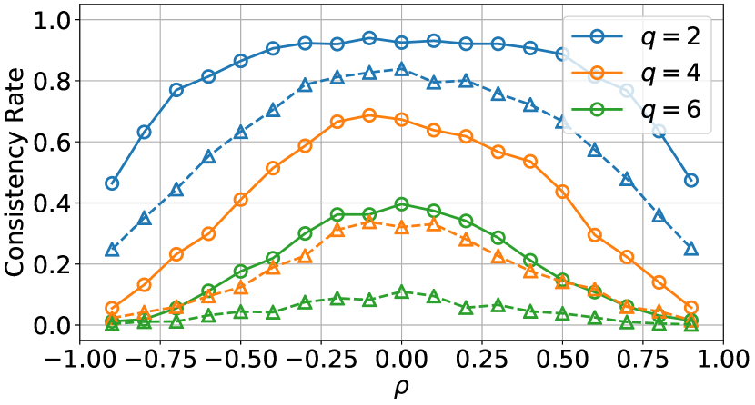
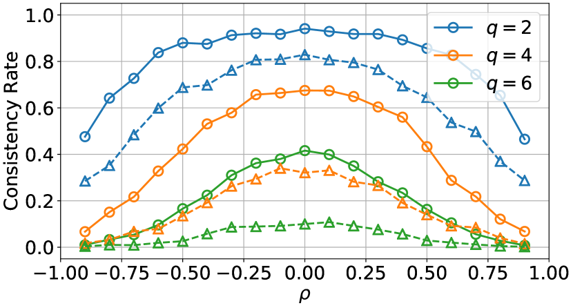
Simulations further confirm this implication.444Appendix C reports more details for the simulations including its computational cost and robustness checks. Consider a two-dimensional (d=2𝑑2d=2) Brownian motion with inter-dimensional correlation ρ𝜌\rho; assume that there are q=#A𝑞#superscript𝐴q=\#A^{*} true predictors in the true model (3), and all of these predictors are signatures of orders no greater than K=4𝐾4K=4. Now, first randomly choose q𝑞q true predictors from all dK+11d1=31superscript𝑑𝐾11𝑑131\frac{d^{K+1}-1}{d-1}=31 signatures; next randomly set each beta coefficient of these true predictors from the standard normal distribution; next generate 100 samples from this true model with error term εnsubscript𝜀𝑛\varepsilon_{n} drawn from a normal distribution with mean zero and standard error 0.01; then run a Lasso regression given by Equation (5) to select predictors based on these 100 samples; and finally check whether the Lasso is sign consistent according to Definition 2. Repeat the above procedure by 1,000 times and calculate the consistency rate, which is defined as the proportion of consistent results among these 1,000 experiments.
Refer to caption
(a) Brownian motion.
Refer to caption
(b) Random walk.
Figure 1: Consistency rates for the Brownian motion and the random walk with different values of inter-dimensional correlation, ρ𝜌\rho, and different numbers of true predictors, q𝑞q. Solid lines correspond to Itô signatures and dashed lines correspond to Stratonovich signatures.

Figure 1 shows the consistency rates for different values of inter-dimensional correlation, ρ𝜌\rho, and different numbers of true predictors, q𝑞q. Figure 1(a) shows the results for the Brownian motion, and Figure 1(b) for its discrete version—the random walk. First, signatures for both Brownian motion and random walk are similar: they both exhibit higher consistency rates when the absolute value of ρ𝜌\rho is small, i.e., when the inter-dimensional correlations of the Brownian motion (random walk) are weak; as the number of true predictors q𝑞q increases, both consistency rates decrease; and finally, consistency rates for Itô signatures are consistently higher than those for Stratonovich signatures, holding other variables constant (ρ𝜌\rho and q𝑞q). All these findings are consistent with our theoretical results.

4.2 Consistency of signatures for OU processes and AR processes

For both the Itô and the Stratonovich signatures of the OU process, we have the following necessary and sufficient condition for the irrepresentable condition. However, it appears difficult to derive the analogue of Proposition 7 for OU processes.

Proposition 8.

For a multi-dimensional OU process given by Equation (11), the irrepresentable condition holds for the correlation matrix of signatures if and only if it holds for both ΨoddsubscriptΨodd\Psi_{\mathrm{odd}} and ΨevensubscriptΨeven\Psi_{\mathrm{even}} given by Equation (10). This result holds for both Itô and Stratonovich signatures.

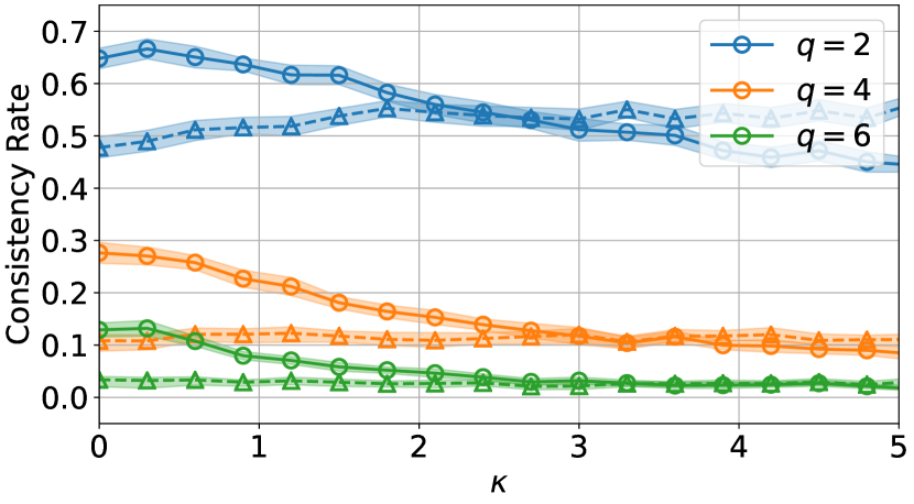
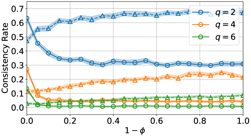
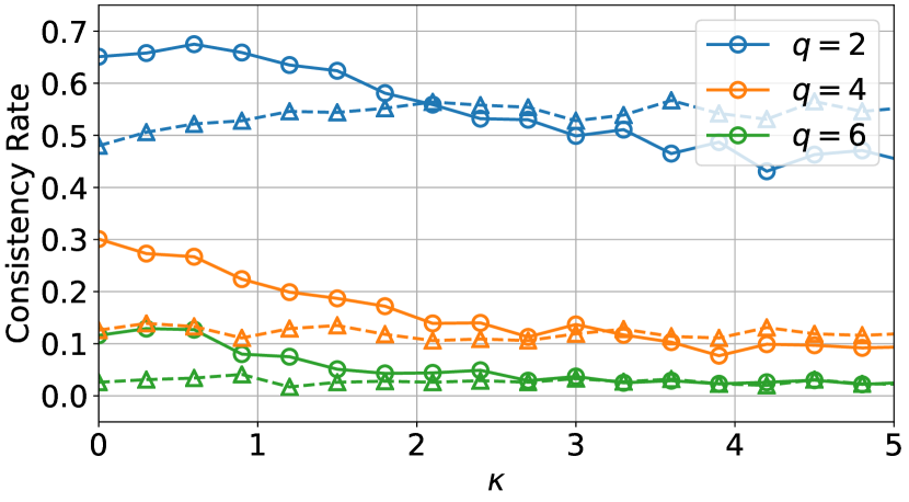
Now we study the impact of different degrees of mean reversion on the consistency of Lasso, for both the OU process and its discrete version—the autoregressive AR(1) model with parameter ϕitalic-ϕ\phi. Recall that higher values of κ𝜅\kappa for the OU process and lower values of ϕitalic-ϕ\phi for the AR(1) model imply stronger levels of mean reversion. We consider two-dimensional OU processes and AR(1) processes, with both dimensions sharing the same parameters (κ𝜅\kappa and ϕitalic-ϕ\phi). The inter-dimensional correlation matrix ΓΓΓsuperscriptΓtop\Gamma\Gamma^{\top} is randomly drawn from the Wishart(2,2)22(2,2) distribution. Other simulation setups are the same as in Section 4.1.
Refer to caption
(a) OU process.
Refer to caption
(b) AR(1) model.
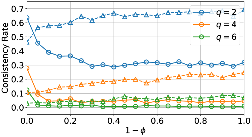
Figure 2: Consistency rates for the OU process and the AR(1) model with different parameters (κ𝜅\kappa and 1ϕ1italic-ϕ1-\phi) and different numbers of true predictors, q𝑞q. Solid lines correspond to Itô signatures and dashed lines correspond to Stratonovich signatures.

Figure 2 shows the simulation results for the consistency rates of both processes. First, the Itô signature reaches the highest consistency rate when κ𝜅\kappa and 1ϕ1italic-ϕ1-\phi approach 00, which correspond respectively to a Brownian motion and a random walk. Second, when the process is sufficiently mean reverting, Stratonovich signatures have higher consistency rates than Itô signatures. Finally, as observed in Section 4.1, Lasso gets less consistent when the number of true predictors q𝑞q increases.

These results suggest that, in practice, for processes that are sufficiently rough or mean reverting [11, 14], using Lasso with Stratonovich signatures will likely lead to higher statistical consistency compared to Itô signatures. More theoretical explanations are provided in Appendix B.

5 Discussion

Consistency and universal nonlinearity.

We have adopted the sign consistency of Lasso [43], defined as whether the Lasso can select all true predictors with correct signs. This restrictive notion of consistency may be relaxed in the context of signatures because the true model is approximated by the linear combination of signatures with some error according to Equation (2). Extensions of the sign consistency for signatures are given in Appendix D. Overall, a lower sign consistency implies poorer performances when using other metrics to measure the performance of feature selections using Lasso, such as the out-of-sample mean squared error. This highlights the significant and practical relevance to study the statistical properties of the signature transform.

Time augmentation.

Time augmentation is a widely used technique in signature-based analysis, which involves adding a time dimension t𝑡t to the original time series, 𝐗tsubscript𝐗𝑡\mathbf{X}_{t} [6, 27]. Time augmentation lowers the consistency rate of Lasso, as presented in Appendix E.

Other feature selection techniques.

While Lasso is a popular feature selection technique, there are also other commonly used techniques, such as the ridge regression [17]. The research on the consistency of signatures using other feature selection techniques is left for further investigation.

6 Conclusion

This paper studies the statistical consistency of Lasso regression for signatures. It finds that consistency is highly dependent on the definition of the signatures and the characteristics of the underlying processes. These findings call for further statistical studies for signature transform before its potential for machine learning can be fully realized.

References

  • [1] Imanol Perez Arribas. Derivatives pricing using signature payoffs. arXiv preprint arXiv:1809.09466, 2018.
  • [2] Peter J Bickel, Ya’acov Ritov, and Alexandre B Tsybakov. Simultaneous analysis of Lasso and Dantzig selector. The Annals of Statistics, pages 1705–1732, 2009.
  • [3] Horatio Boedihardjo, Hao Ni, and Zhongmin Qian. Uniqueness of signature for simple curves. Journal of Functional Analysis, 267(6):1778–1806, 2014.
  • [4] Kuo-Tsai Chen. Iterated integrals and exponential homomorphisms. Proceedings of the London Mathematical Society, 3(1):502–512, 1954.
  • [5] Kuo-Tsai Chen. Integration of paths, geometric invariants and a generalized Baker–Hausdorff formula. Annals of Mathematics, pages 163–178, 1957.
  • [6] Ilya Chevyrev and Andrey Kormilitzin. A primer on the signature method in machine learning. arXiv preprint arXiv:1603.03788, 2016.
  • [7] Ilya Chevyrev and Terry Lyons. Characteristic functions of measures on geometric rough paths. Annals of Probability, 44(6):4049–4082, 2016.
  • [8] Ilya Chevyrev and Harald Oberhauser. Signature moments to characterize laws of stochastic processes. Journal of Machine Learning Research, 23(176):1–42, 2022.
  • [9] Christa Cuchiero, Guido Gazzani, and Sara Svaluto-Ferro. Signature-based models: theory and calibration. arXiv preprint arXiv:2207.13136, 2022.
  • [10] Christa Cuchiero, Francesca Primavera, and Sara Svaluto-Ferro. Universal approximation theorems for continuous functions of càdlàg paths and Lévy-type signature models. arXiv preprint arXiv:2208.02293, 2022.
  • [11] Omar El Euch, Masaaki Fukasawa, and Mathieu Rosenbaum. The microstructural foundations of leverage effect and rough volatility. Finance and Stochastics, 22:241–280, 2018.
  • [12] Adeline Fermanian. Embedding and learning with signatures. Computational Statistics & Data Analysis, 157:107148, 2021.
  • [13] Peter K Friz and Nicolas B Victoir. Multidimensional Stochastic Processes as Rough Paths: Theory and Applications, volume 120. Cambridge University Press, 2010.
  • [14] Jim Gatheral, Thibault Jaisson, and Mathieu Rosenbaum. Volatility is rough. Quantitative Finance, 18(6):933–949, 2018.
  • [15] Lajos Gergely Gyurkó, Terry Lyons, Mark Kontkowski, and Jonathan Field. Extracting information from the signature of a financial data stream. arXiv preprint arXiv:1307.7244, 2013.
  • [16] Ben Hambly and Terry Lyons. Uniqueness for the signature of a path of bounded variation and the reduced path group. Annals of Mathematics, pages 109–167, 2010.
  • [17] Trevor Hastie, Robert Tibshirani, Jerome H Friedman, and Jerome H Friedman. The Elements of Statistical Learning: Data Mining, Inference, and Prediction, volume 2. Springer, 2009.
  • [18] Jasdeep Kalsi, Terry Lyons, and Imanol Perez Arribas. Optimal execution with rough path signatures. SIAM Journal on Financial Mathematics, 11(2):470–493, 2020.
  • [19] Patrick Kidger, Patric Bonnier, Imanol Perez Arribas, Cristopher Salvi, and Terry Lyons. Deep signature transforms. Advances in Neural Information Processing Systems, 32, 2019.
  • [20] Franz J Király and Harald Oberhauser. Kernels for sequentially ordered data. Journal of Machine Learning Research, 20, 2019.
  • [21] Andrey Kormilitzin, Kate EA Saunders, Paul J Harrison, John R Geddes, and Terry Lyons. Detecting early signs of depressive and manic episodes in patients with bipolar disorder using the signature-based model. arXiv preprint arXiv:1708.01206, 2017.
  • [22] Yves Le Jan and Zhongmin Qian. Stratonovich’s signatures of Brownian motion determine Brownian sample paths. Probability Theory and Related Fields, 157(1-2):209–223, 2013.
  • [23] Maud Lemercier, Cristopher Salvi, Theodoros Damoulas, Edwin Bonilla, and Terry Lyons. Distribution regression for sequential data. In International Conference on Artificial Intelligence and Statistics, pages 3754–3762. PMLR, 2021.
  • [24] Daniel Levin, Terry Lyons, and Hao Ni. Learning from the past, predicting the statistics for the future, learning an evolving system. arXiv preprint arXiv:1309.0260, 2016.
  • [25] Chenyang Li, Xin Zhang, and Lianwen Jin. LPSNet: a novel log path signature feature based hand gesture recognition framework. In Proceedings of the IEEE International Conference on Computer Vision Workshops, pages 631–639, 2017.
  • [26] Terry Lyons. Rough paths, signatures and the modelling of functions on streams. arXiv preprint arXiv:1405.4537, 2014.
  • [27] Terry Lyons and Andrew D McLeod. Signature methods in machine learning. arXiv preprint arXiv:2206.14674, 2022.
  • [28] Terry Lyons, Sina Nejad, and Imanol Perez Arribas. Numerical method for model-free pricing of exotic derivatives in discrete time using rough path signatures. Applied Mathematical Finance, 26(6):583–597, 2019.
  • [29] Terry Lyons, Sina Nejad, and Imanol Perez Arribas. Non-parametric pricing and hedging of exotic derivatives. Applied Mathematical Finance, 27(6):457–494, 2020.
  • [30] Terry Lyons, Hao Ni, and Harald Oberhauser. A feature set for streams and an application to high-frequency financial tick data. In Proceedings of the 2014 International Conference on Big Data Science and Computing, pages 1–8, 2014.
  • [31] Terry J Lyons, Michael Caruana, and Thierry Lévy. Differential Equations Driven by Rough Paths. Springer, 2007.
  • [32] James Morrill, Adeline Fermanian, Patrick Kidger, and Terry Lyons. A generalised signature method for multivariate time series feature extraction. arXiv preprint arXiv:2006.00873, 2020.
  • [33] James Morrill, Andrey Kormilitzin, Alejo Nevado-Holgado, Sumanth Swaminathan, Sam Howison, and Terry Lyons. The signature-based model for early detection of sepsis from electronic health records in the intensive care unit. In 2019 Computing in Cardiology (CinC). IEEE, 2019.
  • [34] James H Morrill, Andrey Kormilitzin, Alejo J Nevado-Holgado, Sumanth Swaminathan, Samuel D Howison, and Terry J Lyons. Utilization of the signature method to identify the early onset of sepsis from multivariate physiological time series in critical care monitoring. Critical Care Medicine, 48(10):e976–e981, 2020.
  • [35] Robert Tibshirani. Regression shrinkage and selection via the lasso. Journal of the Royal Statistical Society: Series B (Methodological), 58(1):267–288, 1996.
  • [36] George E Uhlenbeck and Leonard S Ornstein. On the theory of the Brownian motion. Physical Review, 36(5):823, 1930.
  • [37] Martin J Wainwright. Sharp thresholds for high-dimensional and noisy sparsity recovery using l1subscript𝑙1l_{1}-constrained quadratic programming (Lasso). IEEE Transactions on Information Theory, 55(5):2183–2202, 2009.
  • [38] Daniel Wilson-Nunn, Terry Lyons, Anastasia Papavasiliou, and Hao Ni. A path signature approach to online arabic handwriting recognition. In 2018 IEEE 2nd International Workshop on Arabic and Derived Script Analysis and Recognition (ASAR), pages 135–139. IEEE, 2018.
  • [39] Weixin Yang, Lianwen Jin, and Manfei Liu. DeepWriterID: An end-to-end online text-independent writer identification system. IEEE Intelligent Systems, 31(2):45–53, 2016.
  • [40] Weixin Yang, Lianwen Jin, Hao Ni, and Terry Lyons. Rotation-free online handwritten character recognition using dyadic path signature features, hanging normalization, and deep neural network. In 2016 23rd International Conference on Pattern Recognition (ICPR), pages 4083–4088. IEEE, 2016.
  • [41] Weixin Yang, Lianwen Jin, Dacheng Tao, Zecheng Xie, and Ziyong Feng. DropSample: A new training method to enhance deep convolutional neural networks for large-scale unconstrained handwritten Chinese character recognition. Pattern Recognition, 58:190–203, 2016.
  • [42] Weixin Yang, Terry Lyons, Hao Ni, Cordelia Schmid, and Lianwen Jin. Developing the path signature methodology and its application to landmark-based human action recognition. In Stochastic Analysis, Filtering, and Stochastic Optimization: A Commemorative Volume to Honor Mark HA Davis’s Contributions, pages 431–464. Springer, 2022.
  • [43] Peng Zhao and Bin Yu. On model selection consistency of Lasso. The Journal of Machine Learning Research, 7:2541–2563, 2006.

Supplementary Material

Appendix A Technical details for universal nonlinearity of signatures

There are different statements of universal nonlinearity of signatures in the literature, which we summarize in Table 1 in the main paper. The following theorem gives the precise statement of universal nonlinearity proposed in [27].

Theorem 1 (Universal nonlinearity, Theorem 3.1 of [27]).

Let 𝐗tsubscript𝐗𝑡\mathbf{X}_{t} be a dsuperscript𝑑\mathbb{R}^{d}-valued continuous path with p𝑝p-variation, and let 𝒮𝒮\mathcal{S} be a compact subset of signature paths of 𝐗tsubscript𝐗𝑡{\mathbf{X}}_{t} from time 0 to T𝑇T. Assume that f:𝒮:𝑓𝒮f:\mathcal{S}\to\mathbb{R} is a continuous function. Then, for any ε>0𝜀0\varepsilon>0, there exists some linear functional L::𝐿superscriptL:\mathbb{R}^{\infty}\to\mathbb{R} such that for every s𝒮𝑠𝒮s\in\mathcal{S}:

|f(s)L(s)|ε.𝑓𝑠𝐿𝑠𝜀\left|f(s)-L(s)\right|\leq\varepsilon.

The proof of this theorem can be found in [27]. Other versions of universal nonlinearity can be found in, for example, [1, 9, 10, 12, 20, 24, 29].

Appendix B Technical details and examples for the calculation of correlation matrices

This appendix provides details and examples for calculating the correlation structures of signatures. Appendices B.1 and B.2 discuss the Brownian motion and the OU process, respectively.

B.1 Brownian motion

Itô signature.

Propositions 12 in the main paper give explicit formulas for calculating the correlation structure of Itô signatures for Brownian motions. The “recursive order” mentioned in Proposition 2 is defined as follows.

Definition A.1 (Recursive Order).

Consider a d𝑑d-dimensional process 𝐗𝐗\mathbf{X}. We order the indices of all of its 1st order signatures as:

12d.12𝑑1\quad 2\quad\cdots\quad d.

Then, if all k𝑘k-th order signatures are ordered as:

r1r2rdk,subscript𝑟1subscript𝑟2subscript𝑟superscript𝑑𝑘r_{1}\quad r_{2}\quad\cdots\quad r_{d^{k}},

we define the orders of all (k+1)𝑘1(k+1)-th order signatures as:

r1,1r2,1rdk,1r1,2r2,2rdk,2r1,dr2,drdk,d.subscript𝑟11subscript𝑟21subscript𝑟superscript𝑑𝑘1subscript𝑟12subscript𝑟22subscript𝑟superscript𝑑𝑘2subscript𝑟1𝑑subscript𝑟2𝑑subscript𝑟superscript𝑑𝑘𝑑r_{1},1\quad r_{2},1\quad\cdots\quad r_{d^{k}},1\quad r_{1},2\quad r_{2},2\quad\cdots\quad r_{d^{k}},2\quad\cdots\cdots\cdots\quad r_{1},d\quad r_{2},d\quad\cdots\quad r_{d^{k}},d.

For example, for a d=3𝑑3d=3 dimensional process, the recursive order of its signatures is:

  • 1st order: 1231231\quad 2\quad 3

  • 2nd order: 1,12,13,11,22,23,21,32,33,31121311222321323331,1\quad 2,1\quad 3,1\quad 1,2\quad 2,2\quad 3,2\quad 1,3\quad 2,3\quad 3,3

  • 3rd order: 1,1,12,1,13,1,11,2,12,2,13,2,11,3,12,3,13,3,11112113111212213211312313311,1,1\quad 2,1,1\quad 3,1,1\quad 1,2,1\quad 2,2,1\quad 3,2,1\quad 1,3,1\quad 2,3,1\quad 3,3,1
    1,1,22,1,23,1,21,2,22,2,23,2,21,3,22,3,23,3,2112212312122222322132232332~{}~{}~{}~{}~{}~{}~{}~{}~{}~{}~{}~{}~{}~{}~{}~{}~{}~{}1,1,2\quad 2,1,2\quad 3,1,2\quad 1,2,2\quad 2,2,2\quad 3,2,2\quad 1,3,2\quad 2,3,2\quad 3,3,2
    1,1,32,1,33,1,31,2,32,2,33,2,31,3,32,3,33,3,3113213313123223323133233333~{}~{}~{}~{}~{}~{}~{}~{}~{}~{}~{}~{}~{}~{}~{}~{}~{}~{}1,1,3\quad 2,1,3\quad 3,1,3\quad 1,2,3\quad 2,2,3\quad 3,2,3\quad 1,3,3\quad 2,3,3\quad 3,3,3

To provide intuition for Propositions 12 in the main paper, the following two examples show the correlation structures of Itô signatures for 2-dimensional Brownian motions with inter-dimensional correlations ρ=0.6𝜌0.6\rho=0.6 and ρ=0𝜌0\rho=0, respectively.

Example A.1.

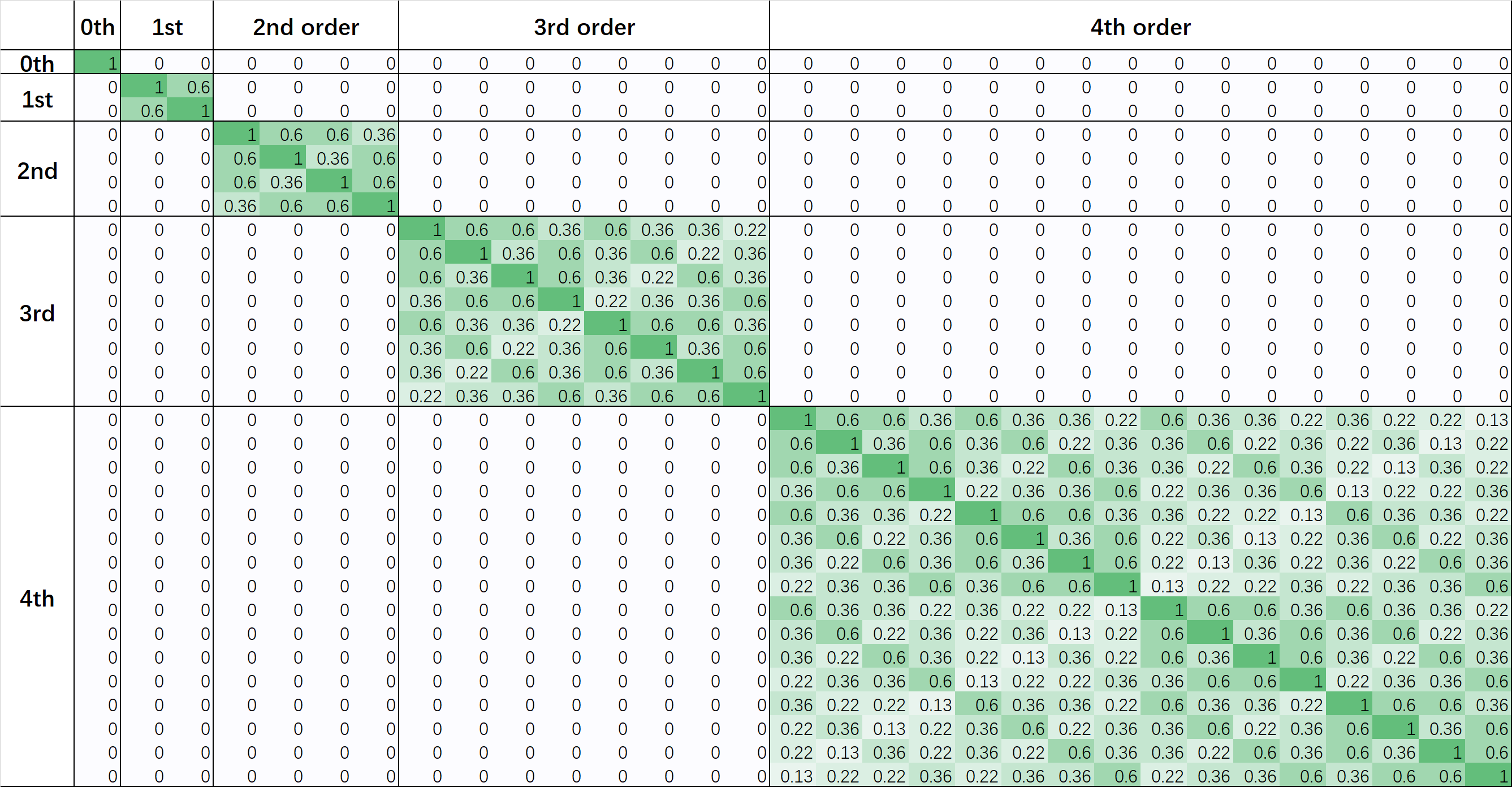
Consider a 2-dimensional Brownian motion given by Equation (6) with inter-dimensional correlation ρ=0.6𝜌0.6\rho=0.6. Figure A.1 shows the correlation matrix of its Itô signatures with orders truncated to 4 calculated using Proposition 1. The figure illustrates Proposition 2—the correlation matrix has a block diagonal structure, and each block of the matrix is the Kronecker product of the inter-dimensional correlation matrix (10.60.61)matrix10.60.61\begin{pmatrix}1&0.6\\ 0.6&1\end{pmatrix}.

Refer to caption
Figure A.1: Correlation matrix of Itô signatures with orders truncated to 4 for a 2-dimensional Brownian motion with inter-dimensional correlation ρ=0.6𝜌0.6\rho=0.6.
Example A.2.

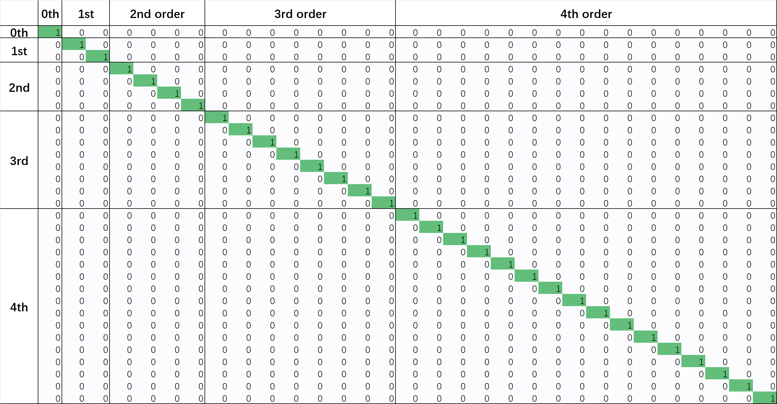
Consider a 2-dimensional Brownian motion given by Equation (6) with inter-dimensional correlation ρ=0𝜌0\rho=0. Figure A.2 shows the correlation matrix of its Itô signatures with orders truncated to 4 calculated using Proposition 1. When ρ=0𝜌0\rho=0, the block diagonal correlation matrix reduces to an identity matrix, indicating that all of its Itô signatures are mutually uncorrelated.
Refer to caption
Figure A.2: Correlation matrix of Itô signatures with orders truncated to 4 for a 2-dimensional Brownian motion with inter-dimensional correlation ρ=0𝜌0\rho=0.
Stratonovich signature.

Propositions 34 in the main paper provide formulas for calculating the correlation structure of Stratonovich signatures for Brownian motions. The following proposition gives recursive formulas for calculating 𝔼[S(𝐗)ti1,,i2n,SS(𝐗)tj1,,j2m,S]𝔼delimited-[]𝑆superscriptsubscript𝐗𝑡subscript𝑖1subscript𝑖2𝑛𝑆𝑆superscriptsubscript𝐗𝑡subscript𝑗1subscript𝑗2𝑚𝑆\mathbb{E}\left[S(\mathbf{X})_{t}^{i_{1},\dots,i_{2n},S}S(\mathbf{X})_{t}^{j_{1},\dots,j_{2m},S}\right] and 𝔼[S(𝐗)ti1,,i2n1,SS(𝐗)tj1,,j2m1,S]𝔼delimited-[]𝑆superscriptsubscript𝐗𝑡subscript𝑖1subscript𝑖2𝑛1𝑆𝑆superscriptsubscript𝐗𝑡subscript𝑗1subscript𝑗2𝑚1𝑆\mathbb{E}\left[S(\mathbf{X})_{t}^{i_{1},\dots,i_{2n-1},S}S(\mathbf{X})_{t}^{j_{1},\dots,j_{2m-1},S}\right], which extends Proposition 3 in the main paper.

Proposition A.1.

Let 𝐗𝐗\mathbf{X} be a d𝑑d-dimensional Brownian motion given by Equation (6). For any l,t0𝑙𝑡0l,t\geq 0 and m,n=1,2,formulae-sequence𝑚𝑛12italic-…m,n=1,2,\dots, define f2n,2m(l,t):=𝔼[S(𝐗)li1,,i2n,SS(𝐗)tj1,,j2m,S]assignsubscript𝑓2𝑛2𝑚𝑙𝑡𝔼delimited-[]𝑆superscriptsubscript𝐗𝑙subscript𝑖1subscript𝑖2𝑛𝑆𝑆superscriptsubscript𝐗𝑡subscript𝑗1subscript𝑗2𝑚𝑆f_{2n,2m}(l,t):=\mathbb{E}\left[S(\mathbf{X})_{l}^{i_{1},\dots,i_{2n},S}S(\mathbf{X})_{t}^{j_{1},\dots,j_{2m},S}\right], we have:

f2n,2m(l,t)subscript𝑓2𝑛2𝑚𝑙𝑡\displaystyle f_{2n,2m}(l,t) =g2n,2m(l,t)+12ρj2m1j2mσj2m1σj2m0tf2n,2m2(l,s)ds,absentsubscript𝑔2𝑛2𝑚𝑙𝑡12subscript𝜌subscript𝑗2𝑚1subscript𝑗2𝑚subscript𝜎subscript𝑗2𝑚1subscript𝜎subscript𝑗2𝑚superscriptsubscript0𝑡subscript𝑓2𝑛2𝑚2𝑙𝑠differential-d𝑠\displaystyle=g_{2n,2m}(l,t)+\frac{1}{2}\rho_{j_{2m-1}j_{2m}}\sigma_{j_{2m-1}}\sigma_{j_{2m}}\int_{0}^{t}f_{2n,2m-2}(l,s)\mathrm{d}s, (A.1)
g2n,2m(l,t)subscript𝑔2𝑛2𝑚𝑙𝑡\displaystyle g_{2n,2m}(l,t) =ρi2nj2mσi2nσj2m0ltf2n1,2m1(s,s)dsabsentsubscript𝜌subscript𝑖2𝑛subscript𝑗2𝑚subscript𝜎subscript𝑖2𝑛subscript𝜎subscript𝑗2𝑚superscriptsubscript0𝑙𝑡subscript𝑓2𝑛12𝑚1𝑠𝑠differential-d𝑠\displaystyle=\rho_{i_{2n}j_{2m}}\sigma_{i_{2n}}\sigma_{j_{2m}}\int_{0}^{l\wedge t}f_{2n-1,2m-1}(s,s)\mathrm{d}s
+12ρi2n1i2nσi2n1σi2n0lg2n2,2m(s,t)ds,12subscript𝜌subscript𝑖2𝑛1subscript𝑖2𝑛subscript𝜎subscript𝑖2𝑛1subscript𝜎subscript𝑖2𝑛superscriptsubscript0𝑙subscript𝑔2𝑛22𝑚𝑠𝑡differential-d𝑠\displaystyle\qquad\qquad+\frac{1}{2}\rho_{i_{2n-1}i_{2n}}\sigma_{i_{2n-1}}\sigma_{i_{2n}}\int_{0}^{l}g_{2n-2,2m}(s,t)\mathrm{d}s, (A.2)

with initial conditions

f0,0(l,t)subscript𝑓00𝑙𝑡\displaystyle f_{0,0}(l,t) =1,absent1\displaystyle=1, (A.3)
g0,2m(l,t)subscript𝑔02𝑚𝑙𝑡\displaystyle g_{0,2m}(l,t) =0.absent0\displaystyle=0. (A.4)

In addition, define f2n1,2m1(l,t):=𝔼[S(𝐗)li1,,i2n1,SS(𝐗)tj1,,j2m1,S]assignsubscript𝑓2𝑛12𝑚1𝑙𝑡𝔼delimited-[]𝑆superscriptsubscript𝐗𝑙subscript𝑖1subscript𝑖2𝑛1𝑆𝑆superscriptsubscript𝐗𝑡subscript𝑗1subscript𝑗2𝑚1𝑆f_{2n-1,2m-1}(l,t):=\mathbb{E}\left[S(\mathbf{X})_{l}^{i_{1},\dots,i_{2n-1},S}S(\mathbf{X})_{t}^{j_{1},\dots,j_{2m-1},S}\right], we have:

f2n1,2m1(l,t)subscript𝑓2𝑛12𝑚1𝑙𝑡\displaystyle f_{2n-1,2m-1}(l,t) =g2n1,2m1(l,t)+12ρj2m2j2m1σj2m2σj2m10tf2n1,2m3(l,s)ds,absentsubscript𝑔2𝑛12𝑚1𝑙𝑡12subscript𝜌subscript𝑗2𝑚2subscript𝑗2𝑚1subscript𝜎subscript𝑗2𝑚2subscript𝜎subscript𝑗2𝑚1superscriptsubscript0𝑡subscript𝑓2𝑛12𝑚3𝑙𝑠differential-d𝑠\displaystyle=g_{2n-1,2m-1}(l,t)+\frac{1}{2}\rho_{j_{2m-2}j_{2m-1}}\sigma_{j_{2m-2}}\sigma_{j_{2m-1}}\int_{0}^{t}f_{2n-1,2m-3}(l,s)\mathrm{d}s, (A.5)
g2n1,2m1(l,t)subscript𝑔2𝑛12𝑚1𝑙𝑡\displaystyle g_{2n-1,2m-1}(l,t) =ρi2n1j2m1σi2n1σj2m10ltf2n2,2m2(s,s)dsabsentsubscript𝜌subscript𝑖2𝑛1subscript𝑗2𝑚1subscript𝜎subscript𝑖2𝑛1subscript𝜎subscript𝑗2𝑚1superscriptsubscript0𝑙𝑡subscript𝑓2𝑛22𝑚2𝑠𝑠differential-d𝑠\displaystyle=\rho_{i_{2n-1}j_{2m-1}}\sigma_{i_{2n-1}}\sigma_{j_{2m-1}}\int_{0}^{l\wedge t}f_{2n-2,2m-2}(s,s)\mathrm{d}s
+12ρi2n2i2n1σi2n2σi2n10lg2n3,2m1(s,t)ds,12subscript𝜌subscript𝑖2𝑛2subscript𝑖2𝑛1subscript𝜎subscript𝑖2𝑛2subscript𝜎subscript𝑖2𝑛1superscriptsubscript0𝑙subscript𝑔2𝑛32𝑚1𝑠𝑡differential-d𝑠\displaystyle\qquad\qquad+\frac{1}{2}\rho_{i_{2n-2}i_{2n-1}}\sigma_{i_{2n-2}}\sigma_{i_{2n-1}}\int_{0}^{l}g_{2n-3,2m-1}(s,t)\mathrm{d}s, (A.6)

with initial conditions

f1,1(l,t)subscript𝑓11𝑙𝑡\displaystyle f_{1,1}(l,t) =ρi1j1σi1σj1(lt),absentsubscript𝜌subscript𝑖1subscript𝑗1subscript𝜎subscript𝑖1subscript𝜎subscript𝑗1𝑙𝑡\displaystyle=\rho_{i_{1}j_{1}}\sigma_{i_{1}}\sigma_{j_{1}}(l\wedge t), (A.7)
g1,2m1(l,t)subscript𝑔12𝑚1𝑙𝑡\displaystyle g_{1,2m-1}(l,t) =ρi1j2m112m1(lt)m1(m1)!σi1k=12m1σjkk=1m1ρj2k1j2k.absentsubscript𝜌subscript𝑖1subscript𝑗2𝑚11superscript2𝑚1superscript𝑙𝑡𝑚1𝑚1subscript𝜎subscript𝑖1superscriptsubscriptproduct𝑘12𝑚1subscript𝜎subscript𝑗𝑘superscriptsubscriptproduct𝑘1𝑚1subscript𝜌subscript𝑗2𝑘1subscript𝑗2𝑘\displaystyle=\rho_{i_{1}j_{2m-1}}\frac{1}{2^{m-1}}\frac{(l\wedge t)^{m-1}}{(m-1)!}\sigma_{i_{1}}\prod_{k=1}^{2m-1}\sigma_{j_{k}}\prod_{k=1}^{m-1}\rho_{j_{2k-1}j_{2k}}. (A.8)

Here, xy𝑥𝑦x\wedge y represents the smaller value between x𝑥x and y𝑦y.

The following two examples show the correlation structures of Stratonovich signatures for 2-dimensional Brownian motions with inter-dimensional correlations ρ=0.6𝜌0.6\rho=0.6 and ρ=0𝜌0\rho=0, respectively, calculated using Propositions 34 in the main paper and Proposition A.1.

Example A.3.

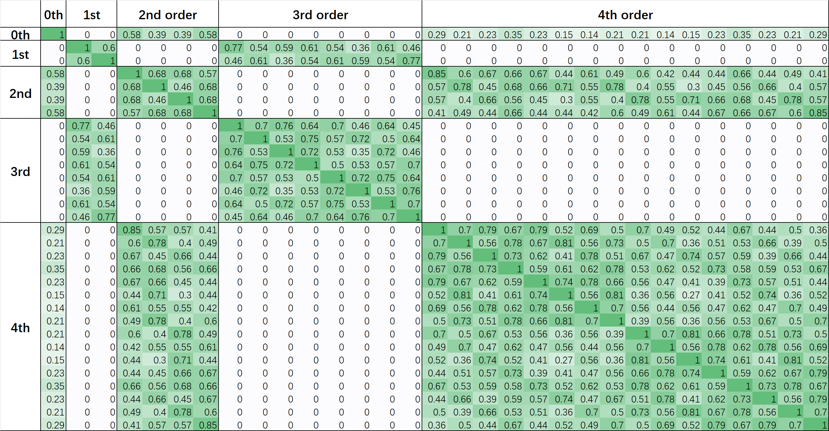
Consider a 2-dimensional Brownian motion given by Equation (6) with inter-dimensional correlation ρ=0.6𝜌0.6\rho=0.6. Figure A.3 shows the correlation matrix of its Stratonovich signatures with orders truncated to 4 calculated using Propositions 3 and A.1. The figure illustrates that the correlation matrix has an odd–even alternating structure.
Refer to caption
Figure A.3: Correlation matrix of Stratonovich signatures with orders truncated to 4 for a 2-dimensional Brownian motion with inter-dimensional correlation ρ=0.6𝜌0.6\rho=0.6.
Example A.4.

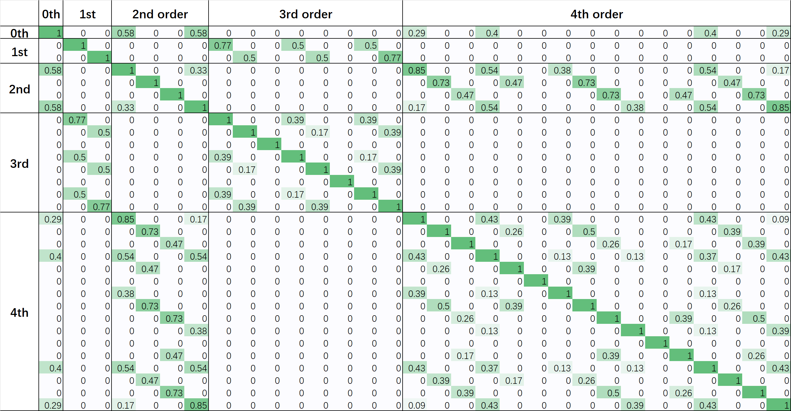
Consider a 2-dimensional Brownian motion given by Equation (6) with inter-dimensional correlation ρ=0𝜌0\rho=0. Figure A.4 shows the correlation matrix of its Stratonovich signatures with orders truncated to 4 calculated using Propositions 3 and A.1. The figure demonstrates that the correlation matrix has an odd–even alternating structure, even though different dimensions of the Brownian motion are mutually independent (ρ=0𝜌0\rho=0). This is different from the result for Itô signatures shown in Example A.2, where all Itô signatures are mutually uncorrelated. Note that this example has the same setup as Example 1 in the main paper.
Refer to caption
Figure A.4: Correlation matrix of Stratonovich signatures with orders truncated to 4 for a 2-dimensional Brownian motion with inter-dimensional correlation ρ=0𝜌0\rho=0.

B.2 OU process

Deriving explicit formulas for calculating the exact correlation between signatures of OU processes (both Itô and Stratonovich) is complicated. Here we provide an example to show the general approach for calculating the correlation. The proof of this example is given in Appendix F, and one can use a similar routine to compute the correlation for other setups of OU processes.

Example A.5.

Consider a 1-dimensional OU process 𝐗t=Ytsubscript𝐗𝑡subscript𝑌𝑡\mathbf{X}_{t}=Y_{t} with a mean reversion speed κ>0𝜅0\kappa>0:

dYt=κYtdt+dWt,Y0=0.formulae-sequencedsubscript𝑌𝑡𝜅subscript𝑌𝑡d𝑡dsubscript𝑊𝑡subscript𝑌00\mathrm{d}Y_{t}=-\kappa Y_{t}\mathrm{d}t+\mathrm{d}W_{t},\quad Y_{0}=0. (A.9)

The correlation coefficients between its 0-th order and 2nd order signatures are

𝔼[S(𝐗)T0,IS(𝐗)T1,1,I]𝔼[S(𝐗)T0,I]2𝔼[S(𝐗)T1,1,I]2𝔼delimited-[]𝑆superscriptsubscript𝐗𝑇0𝐼𝑆superscriptsubscript𝐗𝑇11𝐼𝔼superscriptdelimited-[]𝑆superscriptsubscript𝐗𝑇0𝐼2𝔼superscriptdelimited-[]𝑆superscriptsubscript𝐗𝑇11𝐼2\displaystyle\frac{\mathbb{E}\left[S(\mathbf{X})_{T}^{0,I}S(\mathbf{X})_{T}^{1,1,I}\right]}{\sqrt{\mathbb{E}\left[S(\mathbf{X})_{T}^{0,I}\right]^{2}\mathbb{E}\left[S(\mathbf{X})_{T}^{1,1,I}\right]^{2}}} =2κTe2κT+14κTe2κT+3e4κT6e2κT4κT+3+4κ2T2,absent2𝜅𝑇superscript𝑒2𝜅𝑇14𝜅𝑇superscript𝑒2𝜅𝑇3superscript𝑒4𝜅𝑇6superscript𝑒2𝜅𝑇4𝜅𝑇34superscript𝜅2superscript𝑇2\displaystyle=\frac{-2\kappa T-e^{-2\kappa T}+1}{\sqrt{4\kappa Te^{-2\kappa T}+3e^{-4\kappa T}-6e^{-2\kappa T}-4\kappa T+3+4\kappa^{2}T^{2}}},
𝔼[S(𝐗)T0,SS(𝐗)T1,1,S]𝔼[S(𝐗)T0,S]2𝔼[S(𝐗)T1,1,S]2𝔼delimited-[]𝑆superscriptsubscript𝐗𝑇0𝑆𝑆superscriptsubscript𝐗𝑇11𝑆𝔼superscriptdelimited-[]𝑆superscriptsubscript𝐗𝑇0𝑆2𝔼superscriptdelimited-[]𝑆superscriptsubscript𝐗𝑇11𝑆2\displaystyle\frac{\mathbb{E}\left[S(\mathbf{X})_{T}^{0,S}S(\mathbf{X})_{T}^{1,1,S}\right]}{\sqrt{\mathbb{E}\left[S(\mathbf{X})_{T}^{0,S}\right]^{2}\mathbb{E}\left[S(\mathbf{X})_{T}^{1,1,S}\right]^{2}}} =33,absent33\displaystyle=\frac{\sqrt{3}}{3},

for Itô and Stratonovich signatures, respectively. The proof is provided in Appendix F.

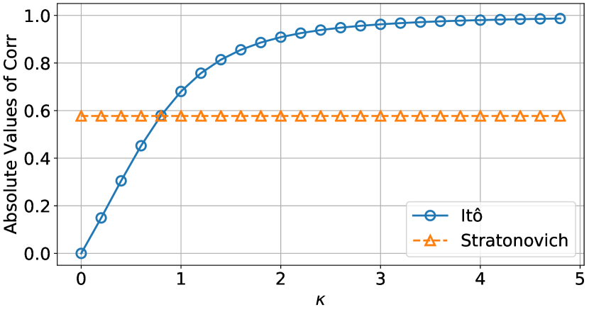
Figure 5(a) shows the absolute values of correlation coefficients between the 0-th order and 2nd order signatures calculated using the formulas above under different values of κ𝜅\kappa. Notably, the correlation for Itô signatures rises with κ𝜅\kappa, while the correlation for Stratonovich signatures remains fixed at 3333\frac{\sqrt{3}}{3}.

Refer to caption
(a) Correlation between the 0-th and the 2nd order signatures.
Refer to caption
(b) Correlation between the first four order signatures.
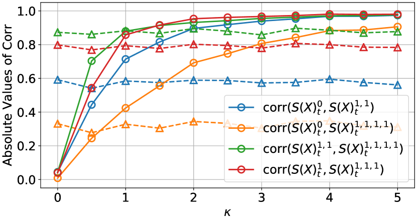
Figure A.5: Absolute values of correlation coefficients between signatures of the 1-dimensional OU process. Solid lines correspond to Itô signatures and dashed lines correspond to Stratonovich signatures.

We further perform simulations to estimate the correlation coefficients for higher-order signatures of the OU process. We generate 10,000 sample paths of the OU process using the methods discussed in Appendix C. For each path, we calculate the corresponding signatures and then estimate the sample correlation matrix based on the 10,000 simulated samples. Figure 5(b) shows the simulation results for the absolute values of correlation coefficients between the first four order signatures under different values of κ𝜅\kappa. Consistent with the observation in Figure 5(a), the correlation for Itô signatures rises with κ𝜅\kappa, while the correlation for Stratonovich signatures remains relatively stable. Notably, the correlations for Itô signatures are zero when κ=0𝜅0\kappa=0, which reduces to a Brownian motion. In addition, when κ𝜅\kappa is sufficiently large, the absolute values of correlation coefficients for Itô signatures exceed those for Stratonovich signatures.

Recall that the irrepresentable condition, as defined in Definition 3, illustrates that a higher correlation generally leads to poorer consistency. Therefore, based on Example A.5, we can expect that the Lasso is more consistent when using Itô signatures for small values of κ𝜅\kappa (weaker mean reversion), and more consistent when using Stratonovich signatures for large values of κ𝜅\kappa (stronger mean reversion). This provides a theoretical explanation for our observations in Section 4.2 of the main paper: When processes are sufficiently rough or mean reverting [11, 14], using Lasso with Stratonovich signatures will likely lead to higher statistical consistency compared to Itô signatures.

Appendix C Details for simulations

This appendix provides additional technical details, computational cost, and robustness checks for the simulations conducted in this paper.

C.1 More technical details

Simulation of processes.

We simulate the i𝑖i-th dimension of the Brownian motion, Wtisuperscriptsubscript𝑊𝑡𝑖W_{t}^{i}, and OU process, Ytisuperscriptsubscript𝑌𝑡𝑖Y_{t}^{i}, by discretizing the stochastic differential equations of the processes using the Euler–Maruyama method:

  • Brownian motion: Wtk+1i=Wtki+Δtεkisuperscriptsubscript𝑊subscript𝑡𝑘1𝑖superscriptsubscript𝑊subscript𝑡𝑘𝑖Δ𝑡superscriptsubscript𝜀𝑘𝑖W_{t_{k+1}}^{i}=W_{t_{k}}^{i}+\sqrt{\Delta t}\varepsilon_{k}^{i}, W0i=0superscriptsubscript𝑊0𝑖0W_{0}^{i}=0;

  • OU process: Ytk+1i=YtkiκiYtkiΔt+Δtεkisuperscriptsubscript𝑌subscript𝑡𝑘1𝑖superscriptsubscript𝑌subscript𝑡𝑘𝑖subscript𝜅𝑖superscriptsubscript𝑌subscript𝑡𝑘𝑖Δ𝑡Δ𝑡superscriptsubscript𝜀𝑘𝑖Y_{t_{k+1}}^{i}=Y_{t_{k}}^{i}-\kappa_{i}Y_{t_{k}}^{i}\Delta t+\sqrt{\Delta t}\varepsilon_{k}^{i}, Y0i=0superscriptsubscript𝑌0𝑖0Y_{0}^{i}=0.

Here, 0=t0<t1<<tN=T0subscript𝑡0subscript𝑡1subscript𝑡𝑁𝑇0=t_{0}<t_{1}<\dots<t_{N}=T, tk+1tk=Δt=T/Nsubscript𝑡𝑘1subscript𝑡𝑘Δ𝑡𝑇𝑁t_{k+1}-t_{k}=\Delta t=T/N for any k𝑘k, and εkisuperscriptsubscript𝜀𝑘𝑖\varepsilon_{k}^{i} are randomly drawn from the standard normal distribution. The number of steps is set to N=100𝑁100N=100.

The i𝑖i-th dimension of the random walk and AR(1) model, both denoted by Ztisuperscriptsubscript𝑍𝑡𝑖Z_{t}^{i}, are simulated using the following formulas:

  • Random walk: Ztk+1i=Ztki+ekisuperscriptsubscript𝑍subscript𝑡𝑘1𝑖superscriptsubscript𝑍subscript𝑡𝑘𝑖superscriptsubscript𝑒𝑘𝑖Z_{t_{k+1}}^{i}=Z_{t_{k}}^{i}+e_{k}^{i}, Z0i=0superscriptsubscript𝑍0𝑖0Z_{0}^{i}=0;

  • AR(1) model: Ztk+1i=ϕiZtki+εkisuperscriptsubscript𝑍subscript𝑡𝑘1𝑖subscriptitalic-ϕ𝑖superscriptsubscript𝑍subscript𝑡𝑘𝑖superscriptsubscript𝜀𝑘𝑖Z_{t_{k+1}}^{i}=\phi_{i}Z_{t_{k}}^{i}+\varepsilon_{k}^{i}, Z0i=0superscriptsubscript𝑍0𝑖0Z_{0}^{i}=0.

Here, 0=t0<t1<<tN=T0subscript𝑡0subscript𝑡1subscript𝑡𝑁𝑇0=t_{0}<t_{1}<\dots<t_{N}=T, tk+1tk=Δt=T/Nsubscript𝑡𝑘1subscript𝑡𝑘Δ𝑡𝑇𝑁t_{k+1}-t_{k}=\Delta t=T/N for any k𝑘k, ekisuperscriptsubscript𝑒𝑘𝑖e_{k}^{i} are randomly drawn from the following distribution:

(eki=+1)=(eki=1)=0.5,superscriptsubscript𝑒𝑘𝑖1superscriptsubscript𝑒𝑘𝑖10.5\mathbb{P}(e_{k}^{i}=+1)=\mathbb{P}(e_{k}^{i}=-1)=0.5,

and εkisuperscriptsubscript𝜀𝑘𝑖\varepsilon_{k}^{i} are randomly drawn from the standard normal distribution. The number of steps is set to N=100𝑁100N=100.

After simulating each dimension of the processes, we simulate the inter-dimensional correlation between different dimensions of the processes using the Cholesky decomposition. Specifically, we set the inter-dimensional correlation matrix ΓΓΓsuperscriptΓtop\Gamma\Gamma^{\top} based on the setups described in the main paper and calculate ΓΓ\Gamma using the Cholesky decomposition. Finally, we generate 𝐗𝐗\mathbf{X} using Equations (6) or (11).

In all of our simulations, we set the length of the processes to T=1𝑇1T=1, and the initial values of the processes to zero. These choices have no impact on the results because the signatures of a path 𝐗𝐗\mathbf{X} are invariant under a time reparametrization and a shift of the starting point of 𝐗𝐗\mathbf{X}, see, for example, [6].

Calculation of integrals.

The calculation of Itô and Stratonovich signatures requires the calculation of Itô and Stratonovich integrals. By definition, these integrals are computed using the following schemes:

  • Itô integral: 0TAtdBtk=0N1Atk(Btk+1Btk)superscriptsubscript0𝑇subscript𝐴𝑡differential-dsubscript𝐵𝑡superscriptsubscript𝑘0𝑁1subscript𝐴subscript𝑡𝑘subscript𝐵subscript𝑡𝑘1subscript𝐵subscript𝑡𝑘\int_{0}^{T}A_{t}\mathrm{d}B_{t}\approx\sum_{k=0}^{N-1}A_{t_{k}}(B_{t_{k+1}}-B_{t_{k}});

  • Stratonovich integral: 0TAtdBtk=0N112(Atk+Atk+1)(Btk+1Btk)superscriptsubscript0𝑇subscript𝐴𝑡differential-dsubscript𝐵𝑡superscriptsubscript𝑘0𝑁112subscript𝐴subscript𝑡𝑘subscript𝐴subscript𝑡𝑘1subscript𝐵subscript𝑡𝑘1subscript𝐵subscript𝑡𝑘\int_{0}^{T}A_{t}\circ\mathrm{d}B_{t}\approx\sum_{k=0}^{N-1}\frac{1}{2}(A_{t_{k}}+A_{t_{k+1}})(B_{t_{k+1}}-B_{t_{k}}).

Here, we set 0=t0<t1<<tN=T0subscript𝑡0subscript𝑡1subscript𝑡𝑁𝑇0=t_{0}<t_{1}<\dots<t_{N}=T and tk+1tk=Δt=T/Nsubscript𝑡𝑘1subscript𝑡𝑘Δ𝑡𝑇𝑁t_{k+1}-t_{k}=\Delta t=T/N for any k𝑘k.

C.2 Computational details

  • The simulations are implemented using Python 3.7.

  • The simulations are run on a laptop with an Intel(R) Core(TM) i7-9750H CPU @ 2.60GHz.

  • The random seed is set to 0 for reproducibility.

  • The Lasso regressions are performed using the sklearn.linear_model.lars_path package.

  • Each individual experiment, including generating 100 paths, calculating their signatures, and performing the Lasso regression, can be completed within one second.

C.3 Robustness checks

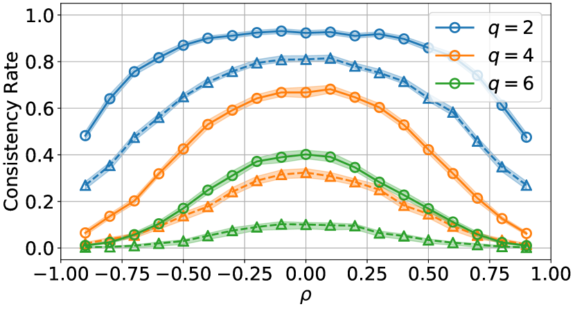
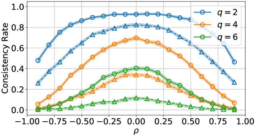
To show the robustness of our simulations shown in Figures 1 and 2 in Section 4 of the main paper, we present Figures A.6 and A.7, which include confidence intervals (shaded regions) for the estimated consistency rates of the Brownian motion/random walk and OU process/AR(1) model, respectively.

In Figures A.6 and A.7, we estimate the consistency rate by repeating the procedure described in Section 4 100 times, and this process is repeated 30 times to obtain the confidence interval for the estimation. Thus, these confidence intervals are based on 30 estimations of the consistency rate, with each estimation calculated using 100 experiments.
Refer to caption
(a) Brownian motion.
Refer to caption
(b) Random walk.
Figure A.6: Consistency rates for the Brownian motion and the random walk with different values of inter-dimensional correlation, ρ𝜌\rho, and different numbers of true predictors, q𝑞q. Solid lines correspond to Itô signatures and dashed lines correspond to Stratonovich signatures. Shaded regions are confidence intervals of the experiments.
Refer to caption
(a) OU process.
Refer to caption
(b) AR(1) model.
Figure A.7: Consistency rates for the OU process and the AR(1) model with different parameters (κ𝜅\kappa and 1ϕ1italic-ϕ1-\phi) and different numbers of true predictors, q𝑞q. Solid lines correspond to Itô signatures and dashed lines correspond to Stratonovich signatures. Shaded regions are confidence intervals of the experiments.

We observe that the confidence intervals of the consistency rates shown in Figures A.6 and A.7 are narrow. Moreover, the observations made in Figures 1 and 2 are consistent with the results presented here, further confirming the robustness of our findings.

Appendix D Extensions of the definition of consistency

As remarked in Section 5 of the main paper, the sign consistency may be too restrictive and can be relaxed in the context of signatures. This appendix provides numerical experiments that explore several extensions of consistency measures for signatures.

D.1 Precision, recall, and F1-score

One possible approach for extending the definition of consistency is to use precision, recall, and the F1-score to evaluate the performance of the Lasso regression in selecting true predictors.

In particular, for a given tuning parameter λ𝜆\lambda in the Lasso regression, Equation (5), let A(λ)𝐴𝜆A(\lambda) denote the set of selected predictors based on the Lasso:

A(λ)=k=0K{(i1,,ik):β~i1,,ik(λ)0},𝐴𝜆superscriptsubscript𝑘0𝐾conditional-setsubscript𝑖1subscript𝑖𝑘subscript~𝛽subscript𝑖1subscript𝑖𝑘𝜆0A(\lambda)=\bigcup_{k=0}^{K}\{(i_{1},\dots,i_{k}):\tilde{\beta}_{i_{1},\dots,i_{k}}(\lambda)\neq 0\},

where β~i1,,ik(λ)subscript~𝛽subscript𝑖1subscript𝑖𝑘𝜆\tilde{\beta}_{i_{1},\dots,i_{k}}(\lambda) are beta coefficients estimated using Equation (5). The true predictor set, Asuperscript𝐴A^{*}, is defined in Equation (4). We can calculate the true positive (TP), false positive (FP), true negative (TN), and false negative (TN) counts as follows:

TP(λ)=#A(λ)A,FP(λ)=#A(λ)Ac,TN(λ)=#A(λ)cAc,FN(λ)=#A(λ)cA,formulae-sequenceTP𝜆#𝐴𝜆superscript𝐴formulae-sequenceFP𝜆#𝐴𝜆superscript𝐴absent𝑐formulae-sequenceTN𝜆#𝐴superscript𝜆𝑐superscript𝐴absent𝑐FN𝜆#𝐴superscript𝜆𝑐superscript𝐴\text{TP}(\lambda)=\#A(\lambda)\cap A^{*},~{}\text{FP}(\lambda)=\#A(\lambda)\cap A^{*c},~{}\text{TN}(\lambda)=\#A(\lambda)^{c}\cap A^{*c},~{}\text{FN}(\lambda)=\#A(\lambda)^{c}\cap A^{*},

where Acsuperscript𝐴absent𝑐A^{*c} and A(λ)c𝐴superscript𝜆𝑐A(\lambda)^{c} represent the complements of Asuperscript𝐴A^{*} and A(λ)𝐴𝜆A(\lambda), respectively. The precision, recall, and F1-score can then be defined as:

precision(λ)precision𝜆\displaystyle\text{precision}(\lambda) =TP(λ)TP(λ)+FP(λ),absentTP𝜆TP𝜆FP𝜆\displaystyle=\frac{\text{TP}(\lambda)}{\text{TP}(\lambda)+\text{FP}(\lambda)},
recall(λ)recall𝜆\displaystyle\text{recall}(\lambda) =TP(λ)TP(λ)+FN(λ),absentTP𝜆TP𝜆FN𝜆\displaystyle=\frac{\text{TP}(\lambda)}{\text{TP}(\lambda)+\text{FN}(\lambda)},
F1-score(λ)F1-score𝜆\displaystyle\text{F1-score}(\lambda) =21/recall(λ)+1/precision(λ).absent21recall𝜆1precision𝜆\displaystyle=\frac{2}{1/\text{recall}(\lambda)+1/\text{precision}(\lambda)}.

We can then examine the maximum values of precision, recall, and F1-score as we vary the tuning parameter λ𝜆\lambda in the Lasso. These maximum values reflect the best performance in terms of feature selection by the Lasso.

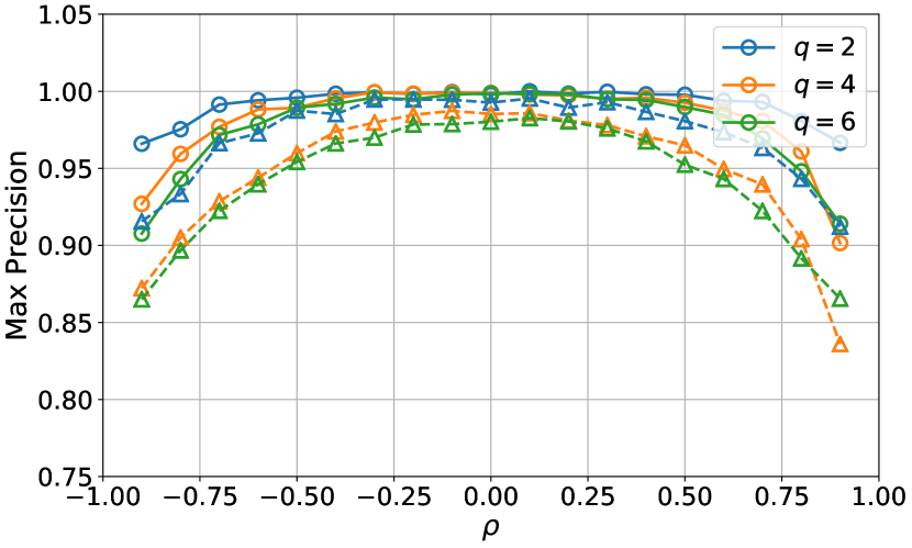
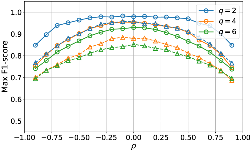
To assess these measures of consistency, we conducted simulations similar to those in Section 4.1 for the Brownian motion. Figure A.8 shows the maximum values of precision, recall, and F1-score for the Brownian motion with different inter-dimensional correlation values (ρ𝜌\rho) and numbers of true predictors (q𝑞q), averaged over 1,000 experiments. The results demonstrate that, similar to the findings in Figure 1, the maximum precision (Figure 8(a)) and F1-score (Figure 8(c)) reach their highest values when ρ=0𝜌0\rho=0, and decrease as the dimensions of the Brownian motion become more correlated. It is also observed that the results for Itô signatures consistently outperform those for Stratonovich signatures. In addition, compared to Figure 1, these alternative measures of consistency exhibit a less pronounced decrease in performance as the absolute value of ρ𝜌\rho increases.

Refer to caption
(a) Maximum precision.
Refer to caption
(b) Maximum recall.
Refer to caption
(c) Maximum F1-score.
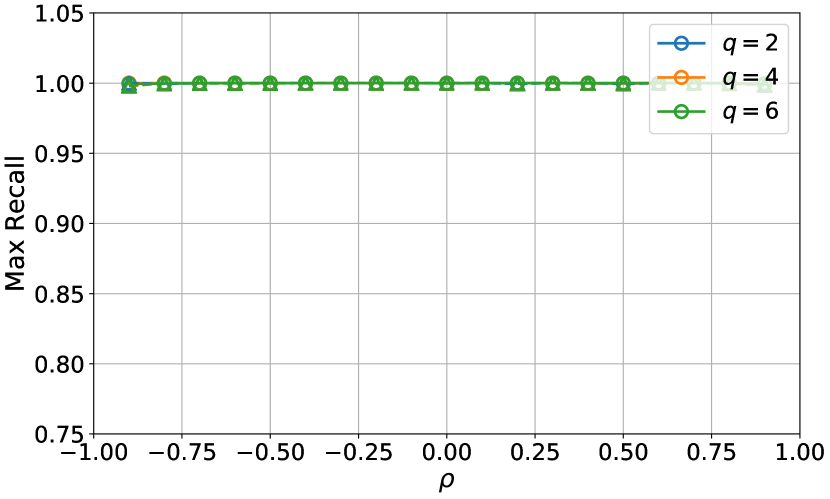
Figure A.8: Maximum values of precision, recall, and F1-score for the Brownian motion with different values of inter-dimensional correlation, ρ𝜌\rho, and different numbers of true predictors, q𝑞q. Solid lines correspond to Itô signatures and dashed lines correspond to Stratonovich signatures.

It is worth noting that the maximum recall rate (Figure 8(b)) remains close to 1 under different parameters. This occurs because none of the predictors are selected by the Lasso when the tuning parameter λ𝜆\lambda is extremely large. As a result, FN(λ)FN𝜆\text{FN}(\lambda) is zero, and recall(λ)recall𝜆\text{recall}(\lambda) is equal to 1. Consequently, the maximum recall rate is not an appropriate measure of consistency in the context of signatures when using the Lasso.

D.2 Out-of-sample R2superscript𝑅2R^{2}

The out-of-sample R2superscript𝑅2R^{2} is a commonly used measure of model performance in machine learning. It generalizes the notion of consistency as it considers the performance of the model on out-of-sample data, rather than solely focusing on the selection of true predictors by the Lasso. This aligns well with practical applications. Furthermore, it is consistent with the concept of universal nonlinearity in signatures, as described by Equation (2). Universal nonlinearity suggests that the true model can be approximated by a linear combination of signatures, without requiring the exact selection of true predictors by the Lasso regression.

We conduct simulations to study the out-of-sample R2superscript𝑅2R^{2} in the context of signatures using Lasso. Consider a two-dimensional (d=2𝑑2d=2) Brownian motion with inter-dimensional correlation ρ𝜌\rho; assume that there are q=#A𝑞#superscript𝐴q=\#A^{*} true predictors in the true model (3), and all of these predictors are signatures of orders no greater than K=4𝐾4K=4. Now, first randomly choose q𝑞q true predictors from all dK+11d1=31superscript𝑑𝐾11𝑑131\frac{d^{K+1}-1}{d-1}=31 signatures; next randomly set each beta coefficient of these true predictors from the standard normal distribution; next generate 200 samples from this true model with error term εnsubscript𝜀𝑛\varepsilon_{n} drawn from a normal distribution with mean zero and standard error 0.0001. We divide the 200 samples into a training set and a test set, with 100 samples assigned to each. Then, we run a Lasso regression given by Equation (5) to select predictors based on the training set. The tuning parameter λ𝜆\lambda is chosen using 5-fold cross-validation. Finally, we calculate the out-of-sample R2superscript𝑅2R^{2} using the chosen λ𝜆\lambda on the test set. We repeat the above procedure by 1,000 times and calculate the average out-of-sample R2superscript𝑅2R^{2}.

Figure A.9 shows the out-of-sample R2superscript𝑅2R^{2} for different values of inter-dimensional correlation, ρ𝜌\rho, and different numbers of true predictors, q𝑞q. We can find that, first, Lasso exhibits lower out-of-sample R2superscript𝑅2R^{2} when the absolute value of ρ𝜌\rho is small, i.e., when the inter-dimensional correlations of the Brownian motion are weak. Second, as the number of true predictors q𝑞q increases, the out-of-sample R2superscript𝑅2R^{2} increases. Finally, Itô signatures have lower out-of-sample R2superscript𝑅2R^{2} than those for Stratonovich signatures, holding other variables constant (ρ𝜌\rho and q𝑞q).

Refer to caption
Figure A.9: Average out-of-sample R2superscript𝑅2R^{2} for the Brownian motion with different values of inter-dimensional correlation, ρ𝜌\rho, and different numbers of true predictors, q𝑞q. Solid lines correspond to Itô signatures and dashed lines correspond to Stratonovich signatures.

All these findings are consistent with our analysis of sign consistency in the main paper. A higher consistency rate corresponds to a higher precision, a higher F1-score, and a lower out-of-sample R2superscript𝑅2R^{2}. This consistency across different metrics reinforces the applicability of our theoretical results when using alternative measures to evaluate the performance of Lasso in the context of signatures. It confirms that the theoretical insights derived from sign consistency extend to other evaluation metrics, demonstrating the robustness and broad applicability of our findings.

Appendix E Time augmentation

Time augmentation is a widely used technique in signature-based analysis, which involves adding a time dimension t𝑡t to the original time series, 𝐗tsubscript𝐗𝑡\mathbf{X}_{t} [6, 27]. In this section, we consider the time-augmented Brownian motion defined as follows:

Definition A.2 (Time-augmented Brownian motion).

𝐗^^𝐗\hat{\mathbf{X}} is a (d+1)𝑑1(d+1)-dimensional time-augmented Brownian motion if it can be expressed as:

𝐗^t=(t,𝐗t)=(t,Xt1,Xt2,,Xtd),subscript^𝐗𝑡superscriptmatrix𝑡superscriptsubscript𝐗𝑡toptopsuperscriptmatrix𝑡superscriptsubscript𝑋𝑡1superscriptsubscript𝑋𝑡2superscriptsubscript𝑋𝑡𝑑top\hat{\mathbf{X}}_{t}=\begin{pmatrix}t,{\mathbf{X}}_{t}^{\top}\end{pmatrix}^{\top}=\begin{pmatrix}t,X_{t}^{1},X_{t}^{2},\dots,X_{t}^{d}\end{pmatrix}^{\top}, (A.10)

where 𝐗t=(Xt1,Xt2,,Xtd)subscript𝐗𝑡superscriptsuperscriptsubscript𝑋𝑡1superscriptsubscript𝑋𝑡2superscriptsubscript𝑋𝑡𝑑top\mathbf{X}_{t}=(X_{t}^{1},X_{t}^{2},\dots,X_{t}^{d})^{\top} is a d𝑑d-dimensional Brownian motion given by Equation (6) in the main paper. For notational simplicity, let Xt0=tsuperscriptsubscript𝑋𝑡0𝑡X_{t}^{0}=t, then

𝐗^t=(Xt0,Xt1,Xt2,,Xtd).subscript^𝐗𝑡superscriptmatrixsuperscriptsubscript𝑋𝑡0superscriptsubscript𝑋𝑡1superscriptsubscript𝑋𝑡2superscriptsubscript𝑋𝑡𝑑top\hat{\mathbf{X}}_{t}=\begin{pmatrix}X_{t}^{0},X_{t}^{1},X_{t}^{2},\dots,X_{t}^{d}\end{pmatrix}^{\top}.

Now we discuss the correlation structure of signatures and the consistency of signatures using Lasso for the time-augmented Brownian motion.

E.1 Correlation structure of signatures for time-augmented Brownian motion

The following proposition shows the moments of Itô signatures for the time-augmented Brownian motion. Note that an index of 0 corresponds to the time dimension, Xt0=tsuperscriptsubscript𝑋𝑡0𝑡X_{t}^{0}=t.

Proposition A.2.

Let 𝐗^^𝐗\hat{\mathbf{X}} be a (d+1)𝑑1(d+1)-dimensional time-augmented Brownian motion given by Equation (A.10). For any l,t0𝑙𝑡0l,t\geq 0 and m,n=1,2,formulae-sequence𝑚𝑛12italic-…m,n=1,2,\dots, fn,m(l,t):=𝔼[S(𝐗^)li1,,in,IS(𝐗^)tj1,,jm,I]assignsubscript𝑓𝑛𝑚𝑙𝑡𝔼delimited-[]𝑆superscriptsubscript^𝐗𝑙subscript𝑖1subscript𝑖𝑛𝐼𝑆superscriptsubscript^𝐗𝑡subscript𝑗1subscript𝑗𝑚𝐼f_{n,m}(l,t):=\mathbb{E}\left[S(\hat{\mathbf{X}})_{l}^{i_{1},\dots,i_{n},I}S(\hat{\mathbf{X}})_{t}^{j_{1},\dots,j_{m},I}\right] can be calculated recursively by:

fn,m(l,t)={0l0tfn1,m1(s,τ)dτds,if in=0,jm=0,0lfn1,m(s,t)ds,if in=0,jm0,0tfn,m1(l,s)ds,if in0,jm=0,ρinjmσinσjm0ltfn1,m1(s,s)ds,if in0,jm0,subscript𝑓𝑛𝑚𝑙𝑡casessuperscriptsubscript0𝑙superscriptsubscript0𝑡subscript𝑓𝑛1𝑚1𝑠𝜏differential-d𝜏differential-d𝑠formulae-sequenceif subscript𝑖𝑛0subscript𝑗𝑚0superscriptsubscript0𝑙subscript𝑓𝑛1𝑚𝑠𝑡differential-d𝑠formulae-sequenceif subscript𝑖𝑛0subscript𝑗𝑚0superscriptsubscript0𝑡subscript𝑓𝑛𝑚1𝑙𝑠differential-d𝑠formulae-sequenceif subscript𝑖𝑛0subscript𝑗𝑚0subscript𝜌subscript𝑖𝑛subscript𝑗𝑚subscript𝜎subscript𝑖𝑛subscript𝜎subscript𝑗𝑚superscriptsubscript0𝑙𝑡subscript𝑓𝑛1𝑚1𝑠𝑠differential-d𝑠formulae-sequenceif subscript𝑖𝑛0subscript𝑗𝑚0f_{n,m}(l,t)=\begin{cases}\int_{0}^{l}\int_{0}^{t}f_{n-1,m-1}(s,\tau)\mathrm{d}\tau\mathrm{d}s,&\text{if }i_{n}=0,j_{m}=0,\\ \int_{0}^{l}f_{n-1,m}(s,t)\mathrm{d}s,&\text{if }i_{n}=0,j_{m}\neq 0,\\ \int_{0}^{t}f_{n,m-1}(l,s)\mathrm{d}s,&\text{if }i_{n}\neq 0,j_{m}=0,\\ \rho_{i_{n}j_{m}}\sigma_{i_{n}}\sigma_{j_{m}}\int_{0}^{l\wedge t}f_{n-1,m-1}(s,s)\mathrm{d}s,&\text{if }i_{n}\neq 0,j_{m}\neq 0,\end{cases}

with initial conditions

f0,m(l,t)subscript𝑓0𝑚𝑙𝑡\displaystyle f_{0,m}(l,t) ={tmm!if j1=j2==jm=0,0,otherwise,absentcasessuperscript𝑡𝑚𝑚if subscript𝑗1subscript𝑗2subscript𝑗𝑚00otherwise\displaystyle=\begin{cases}\frac{t^{m}}{m!}&\text{if }j_{1}=j_{2}=\dots=j_{m}=0,\\ 0,&\text{otherwise},\end{cases}
fn,0(l,t)subscript𝑓𝑛0𝑙𝑡\displaystyle f_{n,0}(l,t) ={tnn!if i1=i2==in=0,0,otherwise.absentcasessuperscript𝑡𝑛𝑛if subscript𝑖1subscript𝑖2subscript𝑖𝑛00otherwise\displaystyle=\begin{cases}\frac{t^{n}}{n!}&\text{if }i_{1}=i_{2}=\dots=i_{n}=0,\\ 0,&\text{otherwise}.\end{cases}

The following proposition shows the moments of Stratonovich signatures for the time-augmented Brownian motion.

Proposition A.3.

Let 𝐗^^𝐗\hat{\mathbf{X}} be a (d+1)𝑑1(d+1)-dimensional time-augmented Brownian motion given by Equation (A.10). For any l,t0𝑙𝑡0l,t\geq 0 and m,n=1,2,formulae-sequence𝑚𝑛12italic-…m,n=1,2,\dots, fn,m(l,t):=𝔼[S(𝐗^)li1,,in,SS(𝐗^)tj1,,jm,S]assignsubscript𝑓𝑛𝑚𝑙𝑡𝔼delimited-[]𝑆superscriptsubscript^𝐗𝑙subscript𝑖1subscript𝑖𝑛𝑆𝑆superscriptsubscript^𝐗𝑡subscript𝑗1subscript𝑗𝑚𝑆f_{n,m}(l,t):=\mathbb{E}\left[S(\hat{\mathbf{X}})_{l}^{i_{1},\dots,i_{n},S}S(\hat{\mathbf{X}})_{t}^{j_{1},\dots,j_{m},S}\right] can be calculated recursively by:

fn,m(l,t)=subscript𝑓𝑛𝑚𝑙𝑡absent\displaystyle f_{n,m}(l,t)=
{0l0tfn1,m1(s,τ)dτds,if in=0,jm=0,0lfn1,m(s,t)ds,if in=0,jm0,ρinjmσinσjm0ltfn1,m1(s,s)ds,if in0,jm0,in1=0,jm1=0,ρinjmσinσjm0ltfn1,m1(s,s)ds+12ρin1inσin1σin0lgn2,m(s,t)ds,if in0,jm0,in10,jm1=0,ρinjmσinσjm0ltfn1,m1(s,s)ds+12ρin1inσin1σin0lgn2,m(s,t)ds+12ρjm1jmσjm1σjm0tg~m2,n(s,l)ds+14ρin1inσin1σinρjm1jmσjm1σjm0l0tfn2,m2(s,τ)dτds,if in0,jm0,in10,jm10,\displaystyle\begin{cases}\int_{0}^{l}\int_{0}^{t}f_{n-1,m-1}(s,\tau)\mathrm{d}\tau\mathrm{d}s,&\text{if }i_{n}=0,j_{m}=0,\\ \int_{0}^{l}f_{n-1,m}(s,t)\mathrm{d}s,&\text{if }i_{n}=0,j_{m}\neq 0,\\ \rho_{i_{n}j_{m}}\sigma_{i_{n}}\sigma_{j_{m}}\int_{0}^{l\wedge t}f_{n-1,m-1}(s,s)\mathrm{d}s,&\text{if }i_{n}\neq 0,j_{m}\neq 0,i_{n-1}=0,j_{m-1}=0,\\ \rho_{i_{n}j_{m}}\sigma_{i_{n}}\sigma_{j_{m}}\int_{0}^{l\wedge t}f_{n-1,m-1}(s,s)\mathrm{d}s&\\ ~{}~{}~{}+\frac{1}{2}\rho_{i_{n-1}i_{n}}\sigma_{i_{n-1}}\sigma_{i_{n}}\int_{0}^{l}g_{n-2,m}(s,t)\mathrm{d}s,&\text{if }i_{n}\neq 0,j_{m}\neq 0,i_{n-1}\neq 0,j_{m-1}=0,\\ \rho_{i_{n}j_{m}}\sigma_{i_{n}}\sigma_{j_{m}}\int_{0}^{l\wedge t}f_{n-1,m-1}(s,s)\mathrm{d}s&\\ ~{}~{}~{}+\frac{1}{2}\rho_{i_{n-1}i_{n}}\sigma_{i_{n-1}}\sigma_{i_{n}}\int_{0}^{l}g_{n-2,m}(s,t)\mathrm{d}s&\\ ~{}~{}~{}+\frac{1}{2}\rho_{j_{m-1}j_{m}}\sigma_{j_{m-1}}\sigma_{j_{m}}\int_{0}^{t}\tilde{g}_{m-2,n}(s,l)\mathrm{d}s&\\ ~{}~{}~{}+\frac{1}{4}\rho_{i_{n-1}i_{n}}\sigma_{i_{n-1}}\sigma_{i_{n}}\rho_{j_{m-1}j_{m}}\sigma_{j_{m-1}}\sigma_{j_{m}}&\\ ~{}~{}~{}~{}~{}~{}~{}~{}~{}~{}~{}~{}~{}~{}~{}~{}~{}~{}~{}~{}~{}~{}~{}~{}~{}~{}~{}~{}~{}~{}~{}~{}~{}\cdot\int_{0}^{l}\int_{0}^{t}f_{n-2,m-2}(s,\tau)\mathrm{d}\tau\mathrm{d}s,&\text{if }i_{n}\neq 0,j_{m}\neq 0,i_{n-1}\neq 0,j_{m-1}\neq 0,\\ \end{cases}
gn,m(l,t)=subscript𝑔𝑛𝑚𝑙𝑡absent\displaystyle g_{n,m}(l,t)=
{0lgn1,m(s,t)ds,if in=0,ρinjmσinσjm0ltfn1,m1(s,s)ds+12ρin1inσin1σin0lgn2,m(s,t)ds,if in0,casessuperscriptsubscript0𝑙subscript𝑔𝑛1𝑚𝑠𝑡differential-d𝑠if subscript𝑖𝑛0subscript𝜌subscript𝑖𝑛subscript𝑗𝑚subscript𝜎subscript𝑖𝑛subscript𝜎subscript𝑗𝑚superscriptsubscript0𝑙𝑡subscript𝑓𝑛1𝑚1𝑠𝑠differential-d𝑠12subscript𝜌subscript𝑖𝑛1subscript𝑖𝑛subscript𝜎subscript𝑖𝑛1subscript𝜎subscript𝑖𝑛superscriptsubscript0𝑙subscript𝑔𝑛2𝑚𝑠𝑡differential-d𝑠if subscript𝑖𝑛0\displaystyle\begin{cases}\int_{0}^{l}g_{n-1,m}(s,t)\mathrm{d}s,&\text{if }i_{n}=0,\\ \rho_{i_{n}j_{m}}\sigma_{i_{n}}\sigma_{j_{m}}\int_{0}^{l\wedge t}f_{n-1,m-1}(s,s)\mathrm{d}s+\frac{1}{2}\rho_{i_{n-1}i_{n}}\sigma_{i_{n-1}}\sigma_{i_{n}}\int_{0}^{l}g_{n-2,m}(s,t)\mathrm{d}s,&\text{if }i_{n}\neq 0,\end{cases}
g~m,n(t,l)=subscript~𝑔𝑚𝑛𝑡𝑙absent\displaystyle\tilde{g}_{m,n}(t,l)=
{0tg~m1,n(s,l)ds,if jm=0,ρinjmσinσjm0ltfn1,m1(s,s)ds+12ρjm1jmσjm1σjm0tg~m2,n(s,l)ds,if jm0,casessuperscriptsubscript0𝑡subscript~𝑔𝑚1𝑛𝑠𝑙differential-d𝑠if subscript𝑗𝑚0subscript𝜌subscript𝑖𝑛subscript𝑗𝑚subscript𝜎subscript𝑖𝑛subscript𝜎subscript𝑗𝑚superscriptsubscript0𝑙𝑡subscript𝑓𝑛1𝑚1𝑠𝑠differential-d𝑠12subscript𝜌subscript𝑗𝑚1subscript𝑗𝑚subscript𝜎subscript𝑗𝑚1subscript𝜎subscript𝑗𝑚superscriptsubscript0𝑡subscript~𝑔𝑚2𝑛𝑠𝑙differential-d𝑠if subscript𝑗𝑚0\displaystyle\begin{cases}\int_{0}^{t}\tilde{g}_{m-1,n}(s,l)\mathrm{d}s,&\text{if }j_{m}=0,\\ \rho_{i_{n}j_{m}}\sigma_{i_{n}}\sigma_{j_{m}}\int_{0}^{l\wedge t}f_{n-1,m-1}(s,s)\mathrm{d}s+\frac{1}{2}\rho_{j_{m-1}j_{m}}\sigma_{j_{m-1}}\sigma_{j_{m}}\int_{0}^{t}\tilde{g}_{m-2,n}(s,l)\mathrm{d}s,&\text{if }j_{m}\neq 0,\end{cases}

with initial conditions

f0,0(l,t)subscript𝑓00𝑙𝑡\displaystyle f_{0,0}(l,t) =1,absent1\displaystyle=1,
g0,m(l,t)subscript𝑔0𝑚𝑙𝑡\displaystyle g_{0,m}(l,t) ={0tf0,m1(l,s)ds,if jm=0,0,if jm0,absentcasessuperscriptsubscript0𝑡subscript𝑓0𝑚1𝑙𝑠differential-d𝑠if subscript𝑗𝑚00if subscript𝑗𝑚0\displaystyle=\begin{cases}\int_{0}^{t}f_{0,m-1}(l,s)\mathrm{d}s,&\text{if }j_{m}=0,\\ 0,&\text{if }j_{m}\neq 0,\end{cases}
g~0,n(l,t)subscript~𝑔0𝑛𝑙𝑡\displaystyle\tilde{g}_{0,n}(l,t) ={0lfn1,0(s,t)ds,if in=0,0,if in0.absentcasessuperscriptsubscript0𝑙subscript𝑓𝑛10𝑠𝑡differential-d𝑠if subscript𝑖𝑛00if subscript𝑖𝑛0\displaystyle=\begin{cases}\int_{0}^{l}f_{n-1,0}(s,t)\mathrm{d}s,&\text{if }i_{n}=0,\\ 0,&\text{if }i_{n}\neq 0.\end{cases}

The following example shows the correlation structures of Itô and Stratonovich signatures for a (1+1)-dimensional time-augmented Brownian motion X^^X\hat{\textbf{X}}.

Example A.6.

Consider a (1+1)-dimensional time-augmented Brownian motion X^^X\hat{\textbf{X}}. Figures A.10 and A.11 show the correlation structures of Itô and Stratonovich signatures of X^^X\hat{\textbf{X}}, respectively, calculated through simulations. In particular, we first simulate 10,000 paths of X^^X\hat{\textbf{X}}, then calculate the signatures of each path, and finally calculate the sample correlation matrix of the signatures.
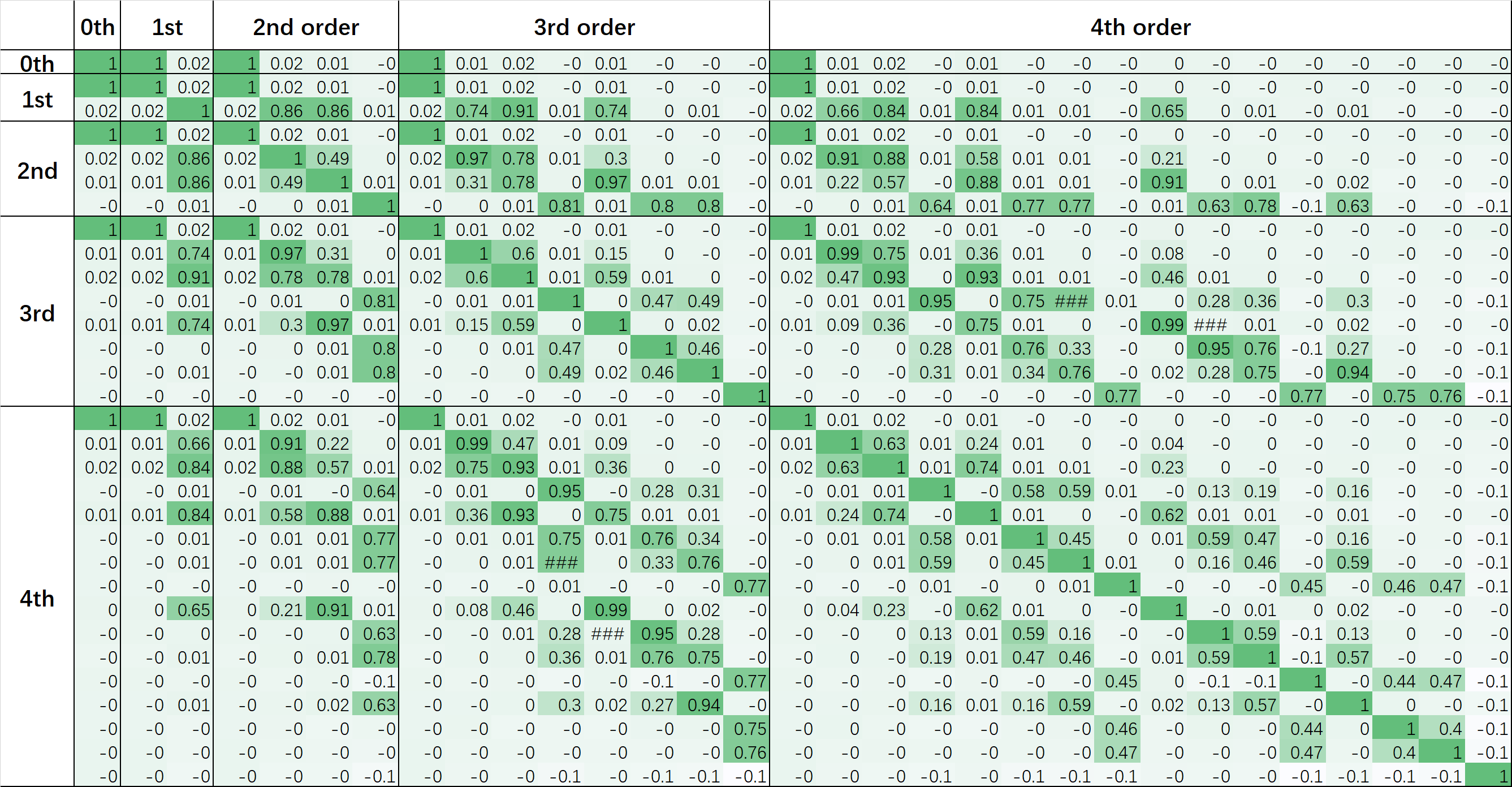
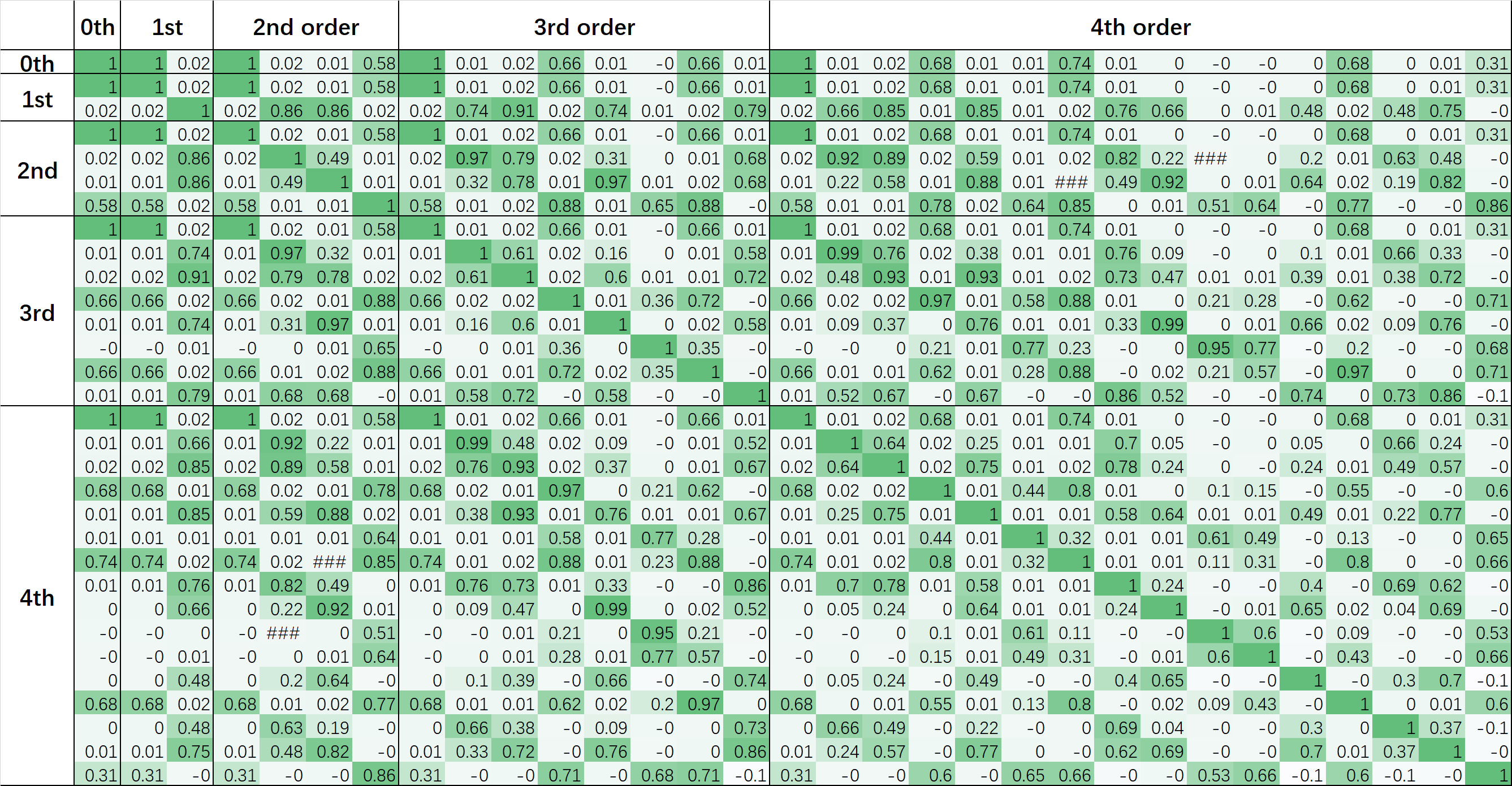
Refer to caption
Figure A.10: Correlation matrix of Itô signatures with orders truncated to 4 for a (1+1)-dimensional time-augmented Brownian motion X^^X\hat{\textbf{X}}.
Refer to caption
Figure A.11: Correlation matrix of Stratonovich signatures with orders truncated to 4 for a (1+1)-dimensional time-augmented Brownian motion X^^X\hat{\textbf{X}}.

From the figures, we can observe that the correlation matrix of the time-augmented Brownian motion does not exhibit the same special structures (block diagonal or odd–even alternating) we observe in the main paper. In addition, the correlation between Stratonovich signatures is generally stronger than that between Itô signatures.

By comparing Figures A.10 and A.11 with Figures A.2 and A.4 in the main paper, we can find that the time augmentation generally increases the correlation between signatures. Therefore, we expect that the time augmentation will lead to a lower consistency rate for Lasso.

E.2 Consistency of signatures for time-augmented Brownian motion

We conduct simulations to study the consistency of signatures using Lasso for the time-augmented Brownian motion.

Consider a (2+1)-dimensional time-augmented Brownian motion X^^X\hat{\textbf{X}}, which is the time-augmented version of a 2-dimensional Brownian motion X. The inter-dimensional correlation of X is ρ𝜌\rho. We perform the same experiment as conducted in Section 4.1 for X^^X\hat{\textbf{X}}.

Figure A.12 shows the consistency rates for different values of inter-dimensional correlation, ρ𝜌\rho, and different numbers of true predictors, q𝑞q. The observations are similar to the results for Brownian motion without time augmentation (Figure 1(a)). In addition, the consistency rates are generally lower when there exists time augmentation (Figure A.12) compared to the case without time augmentation (Figure 1(a)). This is consistent with Example A.6 because time augmentation tends to increase the correlation between signatures, which results in a lower consistency rate.
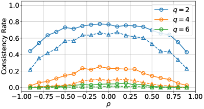
Refer to caption
Figure A.12: Consistency rates for the time-augmented Brownian motion with different values of inter-dimensional correlation, ρ𝜌\rho, and different numbers of true predictors, q𝑞q. Solid lines correspond to Itô signatures and dashed lines correspond to Stratonovich signatures.

In summary, our simulation shows that time augmentation lowers the consistency rate of Lasso.

Appendix F Proofs

This appendix provides the proofs of all theoretical results in this paper.

Proof of Proposition 1.

For the expectation, we have

𝔼[S(𝐗)ti1,,in,I]=𝔼[0tS(𝐗)si1,,in1dXsin]=0𝔼delimited-[]𝑆superscriptsubscript𝐗𝑡subscript𝑖1subscript𝑖𝑛𝐼𝔼delimited-[]superscriptsubscript0𝑡𝑆superscriptsubscript𝐗𝑠subscript𝑖1subscript𝑖𝑛1differential-dsuperscriptsubscript𝑋𝑠subscript𝑖𝑛0\mathbb{E}\left[S(\mathbf{X})_{t}^{i_{1},\dots,i_{n},I}\right]=\mathbb{E}\left[\int_{0}^{t}S(\mathbf{X})_{s}^{i_{1},\dots,i_{n-1}}\mathrm{d}X_{s}^{i_{n}}\right]=0 (A.11)

because the expectation of an Itô integral is zero.

Next we prove 𝔼[S(𝐗)ti1,,in,IS(𝐗)tj1,,jm,I]=0𝔼delimited-[]𝑆superscriptsubscript𝐗𝑡subscript𝑖1subscript𝑖𝑛𝐼𝑆superscriptsubscript𝐗𝑡subscript𝑗1subscript𝑗𝑚𝐼0\mathbb{E}\left[S(\mathbf{X})_{t}^{i_{1},\dots,i_{n},I}S(\mathbf{X})_{t}^{j_{1},\dots,j_{m},I}\right]=0 for mn𝑚𝑛m\neq n by induction. Without loss of generality, we assume that m>n𝑚𝑛m>n. When n=1𝑛1n=1, for any m>1𝑚1m>1, we have

𝔼[S(𝐗)ti1,IS(𝐗)tj1,,jm,I]𝔼delimited-[]𝑆superscriptsubscript𝐗𝑡subscript𝑖1𝐼𝑆superscriptsubscript𝐗𝑡subscript𝑗1subscript𝑗𝑚𝐼\displaystyle\mathbb{E}\left[S(\mathbf{X})_{t}^{i_{1},I}S(\mathbf{X})_{t}^{j_{1},\dots,j_{m},I}\right] =𝔼[(0tdXsi1)(0tS(𝐗)sj1,,jm1dXsjm)]absent𝔼delimited-[]superscriptsubscript0𝑡differential-dsuperscriptsubscript𝑋𝑠subscript𝑖1superscriptsubscript0𝑡𝑆superscriptsubscript𝐗𝑠subscript𝑗1subscript𝑗𝑚1differential-dsuperscriptsubscript𝑋𝑠subscript𝑗𝑚\displaystyle=\mathbb{E}\left[\left(\int_{0}^{t}\mathrm{d}X_{s}^{i_{1}}\right)\left(\int_{0}^{t}S(\mathbf{X})_{s}^{j_{1},\dots,j_{m-1}}\mathrm{d}X_{s}^{j_{m}}\right)\right]
=0t𝔼[S(𝐗)sj1,,jm1,I]ρi1jmσi1σjmds=0,absentsuperscriptsubscript0𝑡𝔼delimited-[]𝑆superscriptsubscript𝐗𝑠subscript𝑗1subscript𝑗𝑚1𝐼subscript𝜌subscript𝑖1subscript𝑗𝑚subscript𝜎subscript𝑖1subscript𝜎subscript𝑗𝑚differential-d𝑠0\displaystyle=\int_{0}^{t}\mathbb{E}\left[S(\mathbf{X})_{s}^{j_{1},\dots,j_{m-1},I}\right]\rho_{i_{1}j_{m}}\sigma_{i_{1}}\sigma_{j_{m}}\mathrm{d}s=0,

where the second equality uses the Itô isometry and the third equality uses Equation (A.11). Now assume that for m>n𝑚𝑛m>n, we have 𝔼[S(𝐗)ti1,,in,IS(𝐗)tj1,,jm,I]=0𝔼delimited-[]𝑆superscriptsubscript𝐗𝑡subscript𝑖1subscript𝑖𝑛𝐼𝑆superscriptsubscript𝐗𝑡subscript𝑗1subscript𝑗𝑚𝐼0\mathbb{E}\left[S(\mathbf{X})_{t}^{i_{1},\dots,i_{n},I}S(\mathbf{X})_{t}^{j_{1},\dots,j_{m},I}\right]=0. Then,

𝔼[S(𝐗)ti1,,in+1,IS(𝐗)tj1,,jm+1,I]𝔼delimited-[]𝑆superscriptsubscript𝐗𝑡subscript𝑖1subscript𝑖𝑛1𝐼𝑆superscriptsubscript𝐗𝑡subscript𝑗1subscript𝑗𝑚1𝐼\displaystyle\mathbb{E}\left[S(\mathbf{X})_{t}^{i_{1},\dots,i_{n+1},I}S(\mathbf{X})_{t}^{j_{1},\dots,j_{m+1},I}\right]
=\displaystyle= 𝔼[(0tS(𝐗)ti1,,in,IdXsin+1)(0tS(𝐗)sj1,,jm,IdXsjm+1)]𝔼delimited-[]superscriptsubscript0𝑡𝑆superscriptsubscript𝐗𝑡subscript𝑖1subscript𝑖𝑛𝐼differential-dsuperscriptsubscript𝑋𝑠subscript𝑖𝑛1superscriptsubscript0𝑡𝑆superscriptsubscript𝐗𝑠subscript𝑗1subscript𝑗𝑚𝐼differential-dsuperscriptsubscript𝑋𝑠subscript𝑗𝑚1\displaystyle\mathbb{E}\left[\left(\int_{0}^{t}S(\mathbf{X})_{t}^{i_{1},\dots,i_{n},I}\mathrm{d}X_{s}^{i_{n+1}}\right)\left(\int_{0}^{t}S(\mathbf{X})_{s}^{j_{1},\dots,j_{m},I}\mathrm{d}X_{s}^{j_{m+1}}\right)\right]
=\displaystyle= 0t𝔼[S(𝐗)ti1,,ik,IS(𝐗)sj1,,jm,I]ρin+1jm+1σin+1σjm+1ds=0.superscriptsubscript0𝑡𝔼delimited-[]𝑆superscriptsubscript𝐗𝑡subscript𝑖1subscript𝑖𝑘𝐼𝑆superscriptsubscript𝐗𝑠subscript𝑗1subscript𝑗𝑚𝐼subscript𝜌subscript𝑖𝑛1subscript𝑗𝑚1subscript𝜎subscript𝑖𝑛1subscript𝜎subscript𝑗𝑚1differential-d𝑠0\displaystyle\int_{0}^{t}\mathbb{E}\left[S(\mathbf{X})_{t}^{i_{1},\dots,i_{k},I}S(\mathbf{X})_{s}^{j_{1},\dots,j_{m},I}\right]\rho_{i_{n+1}j_{m+1}}\sigma_{i_{n+1}}\sigma_{j_{m+1}}\mathrm{d}s=0.

This proves 𝔼[S(𝐗)ti1,,in,IS(𝐗)tj1,,jm,I]=0𝔼delimited-[]𝑆superscriptsubscript𝐗𝑡subscript𝑖1subscript𝑖𝑛𝐼𝑆superscriptsubscript𝐗𝑡subscript𝑗1subscript𝑗𝑚𝐼0\mathbb{E}\left[S(\mathbf{X})_{t}^{i_{1},\dots,i_{n},I}S(\mathbf{X})_{t}^{j_{1},\dots,j_{m},I}\right]=0.

We finally prove 𝔼[S(𝐗)ti1,,in,IS(𝐗)tj1,,jn,I]=tnn!k=1nρikjkσikσjk𝔼delimited-[]𝑆superscriptsubscript𝐗𝑡subscript𝑖1subscript𝑖𝑛𝐼𝑆superscriptsubscript𝐗𝑡subscript𝑗1subscript𝑗𝑛𝐼superscript𝑡𝑛𝑛superscriptsubscriptproduct𝑘1𝑛subscript𝜌subscript𝑖𝑘subscript𝑗𝑘subscript𝜎subscript𝑖𝑘subscript𝜎subscript𝑗𝑘\mathbb{E}\left[S(\mathbf{X})_{t}^{i_{1},\dots,i_{n},I}S(\mathbf{X})_{t}^{j_{1},\dots,j_{n},I}\right]=\frac{t^{n}}{n!}\prod_{k=1}^{n}\rho_{i_{k}j_{k}}\sigma_{i_{k}}\sigma_{j_{k}} by induction. When n=1𝑛1n=1, we have

𝔼[S(𝐗)ti1,IS(𝐗)tj1,I]𝔼delimited-[]𝑆superscriptsubscript𝐗𝑡subscript𝑖1𝐼𝑆superscriptsubscript𝐗𝑡subscript𝑗1𝐼\displaystyle\mathbb{E}\left[S(\mathbf{X})_{t}^{i_{1},I}S(\mathbf{X})_{t}^{j_{1},I}\right]
=\displaystyle= 𝔼[(0tdXsi1)(0tdXsj1)]=0tρi1j1σi1σj1ds=tρi1j1σi1σj1.𝔼delimited-[]superscriptsubscript0𝑡differential-dsuperscriptsubscript𝑋𝑠subscript𝑖1superscriptsubscript0𝑡differential-dsuperscriptsubscript𝑋𝑠subscript𝑗1superscriptsubscript0𝑡subscript𝜌subscript𝑖1subscript𝑗1subscript𝜎subscript𝑖1subscript𝜎subscript𝑗1differential-d𝑠𝑡subscript𝜌subscript𝑖1subscript𝑗1subscript𝜎subscript𝑖1subscript𝜎subscript𝑗1\displaystyle\mathbb{E}\left[\left(\int_{0}^{t}\mathrm{d}X_{s}^{i_{1}}\right)\left(\int_{0}^{t}\mathrm{d}X_{s}^{j_{1}}\right)\right]=\int_{0}^{t}\rho_{i_{1}j_{1}}\sigma_{i_{1}}\sigma_{j_{1}}\mathrm{d}s=t\rho_{i_{1}j_{1}}\sigma_{i_{1}}\sigma_{j_{1}}.

Then, assume that 𝔼[S(𝐗)ti1,,in,IS(𝐗)tj1,,jn,I]=tnn!k=1nρikjkσikσjk𝔼delimited-[]𝑆superscriptsubscript𝐗𝑡subscript𝑖1subscript𝑖𝑛𝐼𝑆superscriptsubscript𝐗𝑡subscript𝑗1subscript𝑗𝑛𝐼superscript𝑡𝑛𝑛superscriptsubscriptproduct𝑘1𝑛subscript𝜌subscript𝑖𝑘subscript𝑗𝑘subscript𝜎subscript𝑖𝑘subscript𝜎subscript𝑗𝑘\mathbb{E}\left[S(\mathbf{X})_{t}^{i_{1},\dots,i_{n},I}S(\mathbf{X})_{t}^{j_{1},\dots,j_{n},I}\right]=\frac{t^{n}}{n!}\prod_{k=1}^{n}\rho_{i_{k}j_{k}}\sigma_{i_{k}}\sigma_{j_{k}}. We have

𝔼[S(𝐗)ti1,,in+1,IS(𝐗)tj1,,jn+1,I]𝔼delimited-[]𝑆superscriptsubscript𝐗𝑡subscript𝑖1subscript𝑖𝑛1𝐼𝑆superscriptsubscript𝐗𝑡subscript𝑗1subscript𝑗𝑛1𝐼\displaystyle\mathbb{E}\left[S(\mathbf{X})_{t}^{i_{1},\dots,i_{n+1},I}S(\mathbf{X})_{t}^{j_{1},\dots,j_{n+1},I}\right]
=\displaystyle= 𝔼[(0tS(𝐗)si1,,in,IdXsin+1)(0tS(𝐗)sj1,,jn,IdXsjn+1)]𝔼delimited-[]superscriptsubscript0𝑡𝑆superscriptsubscript𝐗𝑠subscript𝑖1subscript𝑖𝑛𝐼differential-dsuperscriptsubscript𝑋𝑠subscript𝑖𝑛1superscriptsubscript0𝑡𝑆superscriptsubscript𝐗𝑠subscript𝑗1subscript𝑗𝑛𝐼differential-dsuperscriptsubscript𝑋𝑠subscript𝑗𝑛1\displaystyle\mathbb{E}\left[\left(\int_{0}^{t}S(\mathbf{X})_{s}^{i_{1},\dots,i_{n},I}\mathrm{d}X_{s}^{i_{n+1}}\right)\left(\int_{0}^{t}S(\mathbf{X})_{s}^{j_{1},\dots,j_{n},I}\mathrm{d}X_{s}^{j_{n+1}}\right)\right]
=\displaystyle= 0t𝔼[S(𝐗)si1,,in,IS(𝐗)sj1,,jn,I]ρin+1jn+1σin+1σjn+1dssuperscriptsubscript0𝑡𝔼delimited-[]𝑆superscriptsubscript𝐗𝑠subscript𝑖1subscript𝑖𝑛𝐼𝑆superscriptsubscript𝐗𝑠subscript𝑗1subscript𝑗𝑛𝐼subscript𝜌subscript𝑖𝑛1subscript𝑗𝑛1subscript𝜎subscript𝑖𝑛1subscript𝜎subscript𝑗𝑛1differential-d𝑠\displaystyle\int_{0}^{t}\mathbb{E}\left[S(\mathbf{X})_{s}^{i_{1},\dots,i_{n},I}S(\mathbf{X})_{s}^{j_{1},\dots,j_{n},I}\right]\rho_{i_{n+1}j_{n+1}}\sigma_{i_{n+1}}\sigma_{j_{n+1}}\mathrm{d}s
=\displaystyle= 0t(snn!k=1nρikjkσikσjk)ρin+1jn+1σin+1σjn+1ds=tn+1(n+1)!k=1n+1ρikjkσikσjk.superscriptsubscript0𝑡superscript𝑠𝑛𝑛superscriptsubscriptproduct𝑘1𝑛subscript𝜌subscript𝑖𝑘subscript𝑗𝑘subscript𝜎subscript𝑖𝑘subscript𝜎subscript𝑗𝑘subscript𝜌subscript𝑖𝑛1subscript𝑗𝑛1subscript𝜎subscript𝑖𝑛1subscript𝜎subscript𝑗𝑛1differential-d𝑠superscript𝑡𝑛1𝑛1superscriptsubscriptproduct𝑘1𝑛1subscript𝜌subscript𝑖𝑘subscript𝑗𝑘subscript𝜎subscript𝑖𝑘subscript𝜎subscript𝑗𝑘\displaystyle\int_{0}^{t}\left(\frac{s^{n}}{n!}\prod_{k=1}^{n}\rho_{i_{k}j_{k}}\sigma_{i_{k}}\sigma_{j_{k}}\right)\rho_{i_{n+1}j_{n+1}}\sigma_{i_{n+1}}\sigma_{j_{n+1}}\mathrm{d}s=\frac{t^{n+1}}{(n+1)!}\prod_{k=1}^{n+1}\rho_{i_{k}j_{k}}\sigma_{i_{k}}\sigma_{j_{k}}.

Therefore, 𝔼[S(𝐗)ti1,,in,IS(𝐗)tj1,,jn,I]=tnn!k=1nρikjkσikσjk𝔼delimited-[]𝑆superscriptsubscript𝐗𝑡subscript𝑖1subscript𝑖𝑛𝐼𝑆superscriptsubscript𝐗𝑡subscript𝑗1subscript𝑗𝑛𝐼superscript𝑡𝑛𝑛superscriptsubscriptproduct𝑘1𝑛subscript𝜌subscript𝑖𝑘subscript𝑗𝑘subscript𝜎subscript𝑖𝑘subscript𝜎subscript𝑗𝑘\mathbb{E}\left[S(\mathbf{X})_{t}^{i_{1},\dots,i_{n},I}S(\mathbf{X})_{t}^{j_{1},\dots,j_{n},I}\right]=\frac{t^{n}}{n!}\prod_{k=1}^{n}\rho_{i_{k}j_{k}}\sigma_{i_{k}}\sigma_{j_{k}}. This completes the proof. ∎

Proof of Proposition 2.

By Proposition 1, for any n𝑛n, we have

𝔼[S(𝐗)ti1,,in,IS(𝐗)tj1,,jn,I]𝔼[S(𝐗)ti1,,in,I]2𝔼[S(𝐗)tj1,,jn,I]2=tnn!k=1nρikjkσikσjktnn!k=1nσikσiktnn!k=1nσjkσjk=k=1nρikjk,𝔼delimited-[]𝑆superscriptsubscript𝐗𝑡subscript𝑖1subscript𝑖𝑛𝐼𝑆superscriptsubscript𝐗𝑡subscript𝑗1subscript𝑗𝑛𝐼𝔼superscriptdelimited-[]𝑆superscriptsubscript𝐗𝑡subscript𝑖1subscript𝑖𝑛𝐼2𝔼superscriptdelimited-[]𝑆superscriptsubscript𝐗𝑡subscript𝑗1subscript𝑗𝑛𝐼2superscript𝑡𝑛𝑛superscriptsubscriptproduct𝑘1𝑛subscript𝜌subscript𝑖𝑘subscript𝑗𝑘subscript𝜎subscript𝑖𝑘subscript𝜎subscript𝑗𝑘superscript𝑡𝑛𝑛superscriptsubscriptproduct𝑘1𝑛subscript𝜎subscript𝑖𝑘subscript𝜎subscript𝑖𝑘superscript𝑡𝑛𝑛superscriptsubscriptproduct𝑘1𝑛subscript𝜎subscript𝑗𝑘subscript𝜎subscript𝑗𝑘superscriptsubscriptproduct𝑘1𝑛subscript𝜌subscript𝑖𝑘subscript𝑗𝑘\frac{\mathbb{E}\left[S(\mathbf{X})_{t}^{i_{1},\dots,i_{n},I}S(\mathbf{X})_{t}^{j_{1},\dots,j_{n},I}\right]}{\sqrt{\mathbb{E}\left[S(\mathbf{X})_{t}^{i_{1},\dots,i_{n},I}\right]^{2}\mathbb{E}\left[S(\mathbf{X})_{t}^{j_{1},\dots,j_{n},I}\right]^{2}}}=\frac{\frac{t^{n}}{n!}\prod_{k=1}^{n}\rho_{i_{k}j_{k}}\sigma_{i_{k}}\sigma_{j_{k}}}{\sqrt{\frac{t^{n}}{n!}\prod_{k=1}^{n}\sigma_{i_{k}}\sigma_{i_{k}}\cdot\frac{t^{n}}{n!}\prod_{k=1}^{n}\sigma_{j_{k}}\sigma_{j_{k}}}}=\prod_{k=1}^{n}\rho_{i_{k}j_{k}},

implying that

𝔼[S(𝐗)ti1,IS(𝐗)tj1,I]𝔼[S(𝐗)ti1,I]2𝔼[S(𝐗)tj1,I]2=ρi1j1𝔼delimited-[]𝑆superscriptsubscript𝐗𝑡subscript𝑖1𝐼𝑆superscriptsubscript𝐗𝑡subscript𝑗1𝐼𝔼superscriptdelimited-[]𝑆superscriptsubscript𝐗𝑡subscript𝑖1𝐼2𝔼superscriptdelimited-[]𝑆superscriptsubscript𝐗𝑡subscript𝑗1𝐼2subscript𝜌subscript𝑖1subscript𝑗1\frac{\mathbb{E}\left[S(\mathbf{X})_{t}^{i_{1},I}S(\mathbf{X})_{t}^{j_{1},I}\right]}{\sqrt{\mathbb{E}\left[S(\mathbf{X})_{t}^{i_{1},I}\right]^{2}\mathbb{E}\left[S(\mathbf{X})_{t}^{j_{1},I}\right]^{2}}}=\rho_{i_{1}j_{1}}

and

𝔼[S(𝐗)ti1,,in,IS(𝐗)tj1,,jn,I]𝔼[S(𝐗)ti1,,in,I]2𝔼[S(𝐗)tj1,,jn,I]2=ρinjn𝔼[S(𝐗)ti1,,in1,IS(𝐗)tj1,,jn1,I]𝔼[S(𝐗)ti1,,in1,I]2𝔼[S(𝐗)tj1,,jn1,I]2.𝔼delimited-[]𝑆superscriptsubscript𝐗𝑡subscript𝑖1subscript𝑖𝑛𝐼𝑆superscriptsubscript𝐗𝑡subscript𝑗1subscript𝑗𝑛𝐼𝔼superscriptdelimited-[]𝑆superscriptsubscript𝐗𝑡subscript𝑖1subscript𝑖𝑛𝐼2𝔼superscriptdelimited-[]𝑆superscriptsubscript𝐗𝑡subscript𝑗1subscript𝑗𝑛𝐼2subscript𝜌subscript𝑖𝑛subscript𝑗𝑛𝔼delimited-[]𝑆superscriptsubscript𝐗𝑡subscript𝑖1subscript𝑖𝑛1𝐼𝑆superscriptsubscript𝐗𝑡subscript𝑗1subscript𝑗𝑛1𝐼𝔼superscriptdelimited-[]𝑆superscriptsubscript𝐗𝑡subscript𝑖1subscript𝑖𝑛1𝐼2𝔼superscriptdelimited-[]𝑆superscriptsubscript𝐗𝑡subscript𝑗1subscript𝑗𝑛1𝐼2\frac{\mathbb{E}\left[S(\mathbf{X})_{t}^{i_{1},\dots,i_{n},I}S(\mathbf{X})_{t}^{j_{1},\dots,j_{n},I}\right]}{\sqrt{\mathbb{E}\left[S(\mathbf{X})_{t}^{i_{1},\dots,i_{n},I}\right]^{2}\mathbb{E}\left[S(\mathbf{X})_{t}^{j_{1},\dots,j_{n},I}\right]^{2}}}=\rho_{i_{n}j_{n}}\cdot\frac{\mathbb{E}\left[S(\mathbf{X})_{t}^{i_{1},\dots,i_{n-1},I}S(\mathbf{X})_{t}^{j_{1},\dots,j_{n-1},I}\right]}{\sqrt{\mathbb{E}\left[S(\mathbf{X})_{t}^{i_{1},\dots,i_{n-1},I}\right]^{2}\mathbb{E}\left[S(\mathbf{X})_{t}^{j_{1},\dots,j_{n-1},I}\right]^{2}}}.

This proves the Kronecker product structure given by Equation (8).

Proposition 1 also implies that, for any mn𝑚𝑛m\neq n,

𝔼[S(𝐗)ti1,,in,IS(𝐗)tj1,,jm,I]𝔼[S(𝐗)ti1,,in,I]2𝔼[S(𝐗)tj1,,jm,I]2=0.𝔼delimited-[]𝑆superscriptsubscript𝐗𝑡subscript𝑖1subscript𝑖𝑛𝐼𝑆superscriptsubscript𝐗𝑡subscript𝑗1subscript𝑗𝑚𝐼𝔼superscriptdelimited-[]𝑆superscriptsubscript𝐗𝑡subscript𝑖1subscript𝑖𝑛𝐼2𝔼superscriptdelimited-[]𝑆superscriptsubscript𝐗𝑡subscript𝑗1subscript𝑗𝑚𝐼20\frac{\mathbb{E}\left[S(\mathbf{X})_{t}^{i_{1},\dots,i_{n},I}S(\mathbf{X})_{t}^{j_{1},\dots,j_{m},I}\right]}{\sqrt{\mathbb{E}\left[S(\mathbf{X})_{t}^{i_{1},\dots,i_{n},I}\right]^{2}\mathbb{E}\left[S(\mathbf{X})_{t}^{j_{1},\dots,j_{m},I}\right]^{2}}}=0.

This proves that Itô signatures with different orders are uncorrelated and, therefore, the correlation matrix is block diagonal. This completes the proof. ∎

Proof of Proposition 3.

We omit the proof of Equations

𝔼[S(𝐗)ti1,,i2n1,S]=0𝔼delimited-[]𝑆superscriptsubscript𝐗𝑡subscript𝑖1subscript𝑖2𝑛1𝑆0\mathbb{E}\left[S(\mathbf{X})_{t}^{i_{1},\dots,i_{2n-1},S}\right]=0

and

𝔼[S(𝐗)ti1,,i2n,SS(𝐗)tj1,,j2m1,S]=0𝔼delimited-[]𝑆superscriptsubscript𝐗𝑡subscript𝑖1subscript𝑖2𝑛𝑆𝑆superscriptsubscript𝐗𝑡subscript𝑗1subscript𝑗2𝑚1𝑆0\mathbb{E}\left[S(\mathbf{X})_{t}^{i_{1},\dots,i_{2n},S}S(\mathbf{X})_{t}^{j_{1},\dots,j_{2m-1},S}\right]=0

because they can be proven using a similar approach to the proof Proposition 5. Equation

𝔼[S(𝐗)ti1,,i2n,S]=12ntnn!k=1nρi2k1i2kk=12nσik𝔼delimited-[]𝑆superscriptsubscript𝐗𝑡subscript𝑖1subscript𝑖2𝑛𝑆1superscript2𝑛superscript𝑡𝑛𝑛superscriptsubscriptproduct𝑘1𝑛subscript𝜌subscript𝑖2𝑘1subscript𝑖2𝑘superscriptsubscriptproduct𝑘12𝑛subscript𝜎subscript𝑖𝑘\mathbb{E}\left[S(\mathbf{X})_{t}^{i_{1},\dots,i_{2n},S}\right]=\frac{1}{2^{n}}\frac{t^{n}}{n!}\prod_{k=1}^{n}\rho_{i_{2k-1}i_{2k}}\prod_{k=1}^{2n}\sigma_{i_{k}}

is a corollary of Proposition A.1. ∎

Proof of Proposition 4.

This is a direct corollary of Proposition 3. ∎

Proof of Proposition 5.

We only need to prove that, for an odd number m𝑚m and an even number n𝑛n, we have

𝔼[S(𝐗)ti1,,imS(𝐗)tj1,,jn]=0𝔼delimited-[]𝑆superscriptsubscript𝐗𝑡subscript𝑖1subscript𝑖𝑚𝑆superscriptsubscript𝐗𝑡subscript𝑗1subscript𝑗𝑛0\mathbb{E}\left[S(\mathbf{X})_{t}^{i_{1},\dots,i_{m}}S(\mathbf{X})_{t}^{j_{1},\dots,j_{n}}\right]=0

for any i1,,imsubscript𝑖1subscript𝑖𝑚i_{1},\dots,i_{m} and j1,,jnsubscript𝑗1subscript𝑗𝑛j_{1},\dots,j_{n} taking values in {1,2,,d}12𝑑\{1,2,\dots,d\}. Here the signatures can be defined in the sense of either Itô or Stratonovich.

Consider the reflected OU process, 𝐗~t=𝐗tsubscript~𝐗𝑡subscript𝐗𝑡\tilde{\mathbf{X}}_{t}=-\mathbf{X}_{t}. By definition, 𝐗~tsubscript~𝐗𝑡\tilde{\mathbf{X}}_{t} is also an OU process with the same mean reversion parameter. Therefore, the signatures of 𝐗~tsubscript~𝐗𝑡\tilde{\mathbf{X}}_{t} and 𝐗tsubscript𝐗𝑡{\mathbf{X}}_{t} should have the same distribution. In particular, we have

𝔼[S(𝐗~)ti1,,imS(𝐗~)tj1,,jn]=𝔼[S(𝐗)ti1,,imS(𝐗)tj1,,jn].𝔼delimited-[]𝑆superscriptsubscript~𝐗𝑡subscript𝑖1subscript𝑖𝑚𝑆superscriptsubscript~𝐗𝑡subscript𝑗1subscript𝑗𝑛𝔼delimited-[]𝑆superscriptsubscript𝐗𝑡subscript𝑖1subscript𝑖𝑚𝑆superscriptsubscript𝐗𝑡subscript𝑗1subscript𝑗𝑛\mathbb{E}\left[S(\tilde{\mathbf{X}})_{t}^{i_{1},\dots,i_{m}}S(\tilde{\mathbf{X}})_{t}^{j_{1},\dots,j_{n}}\right]=\mathbb{E}\left[S(\mathbf{X})_{t}^{i_{1},\dots,i_{m}}S({\mathbf{X}})_{t}^{j_{1},\dots,j_{n}}\right]. (A.12)

Now we consider the definition of the signatures:

S(𝐗)ti1,,im=0<t1<<tm<tdXt1i1dXtkim,𝑆superscriptsubscript𝐗𝑡subscript𝑖1subscript𝑖𝑚subscript0subscript𝑡1subscript𝑡𝑚𝑡differential-dsuperscriptsubscript𝑋subscript𝑡1subscript𝑖1differential-dsuperscriptsubscript𝑋subscript𝑡𝑘subscript𝑖𝑚S(\mathbf{X})_{t}^{i_{1},\dots,i_{m}}=\int_{0<t_{1}<\dots<t_{m}<t}\mathrm{d}X_{t_{1}}^{i_{1}}\cdots\mathrm{d}X_{t_{k}}^{i_{m}},

where the integral can be defined in the sense of either Itô or Stratonovich. We therefore have

S(𝐗~)ti1,,im=S(𝐗)ti1,,im𝑆superscriptsubscript~𝐗𝑡subscript𝑖1subscript𝑖𝑚𝑆superscriptsubscript𝐗𝑡subscript𝑖1subscript𝑖𝑚\displaystyle S(\tilde{\mathbf{X}})_{t}^{i_{1},\dots,i_{m}}=S(-{\mathbf{X}})_{t}^{i_{1},\dots,i_{m}} =0<t1<<tm<td(Xt1i1)d(Xtkim)absentsubscript0subscript𝑡1subscript𝑡𝑚𝑡dsuperscriptsubscript𝑋subscript𝑡1subscript𝑖1dsuperscriptsubscript𝑋subscript𝑡𝑘subscript𝑖𝑚\displaystyle=\int_{0<t_{1}<\dots<t_{m}<t}\mathrm{d}(-X_{t_{1}}^{i_{1}})\cdots\mathrm{d}(-X_{t_{k}}^{i_{m}})
=(1)m0<t1<<tm<tdXt1i1dXtkim=(1)mS(𝐗)ti1,,im.absentsuperscript1𝑚subscript0subscript𝑡1subscript𝑡𝑚𝑡differential-dsuperscriptsubscript𝑋subscript𝑡1subscript𝑖1differential-dsuperscriptsubscript𝑋subscript𝑡𝑘subscript𝑖𝑚superscript1𝑚𝑆superscriptsubscript𝐗𝑡subscript𝑖1subscript𝑖𝑚\displaystyle=(-1)^{m}\int_{0<t_{1}<\dots<t_{m}<t}\mathrm{d}X_{t_{1}}^{i_{1}}\cdots\mathrm{d}X_{t_{k}}^{i_{m}}=(-1)^{m}S(\mathbf{X})_{t}^{i_{1},\dots,i_{m}}.

Similarly, we have

S(𝐗~)tj1,,jn=(1)nS(𝐗)tj1,,jn.𝑆superscriptsubscript~𝐗𝑡subscript𝑗1subscript𝑗𝑛superscript1𝑛𝑆superscriptsubscript𝐗𝑡subscript𝑗1subscript𝑗𝑛S(\tilde{\mathbf{X}})_{t}^{j_{1},\dots,j_{n}}=(-1)^{n}S(\mathbf{X})_{t}^{j_{1},\dots,j_{n}}.

Therefore,

𝔼[S(𝐗~)ti1,,imS(𝐗~)tj1,,jn]𝔼delimited-[]𝑆superscriptsubscript~𝐗𝑡subscript𝑖1subscript𝑖𝑚𝑆superscriptsubscript~𝐗𝑡subscript𝑗1subscript𝑗𝑛\displaystyle\mathbb{E}\left[S(\tilde{\mathbf{X}})_{t}^{i_{1},\dots,i_{m}}S(\tilde{\mathbf{X}})_{t}^{j_{1},\dots,j_{n}}\right] =(1)m+n𝔼[S(𝐗)ti1,,imS(𝐗)tj1,,jn]absentsuperscript1𝑚𝑛𝔼delimited-[]𝑆superscriptsubscript𝐗𝑡subscript𝑖1subscript𝑖𝑚𝑆superscriptsubscript𝐗𝑡subscript𝑗1subscript𝑗𝑛\displaystyle=(-1)^{m+n}\mathbb{E}\left[S(\mathbf{X})_{t}^{i_{1},\dots,i_{m}}S({\mathbf{X}})_{t}^{j_{1},\dots,j_{n}}\right]
=𝔼[S(𝐗)ti1,,imS(𝐗)tj1,,jn],absent𝔼delimited-[]𝑆superscriptsubscript𝐗𝑡subscript𝑖1subscript𝑖𝑚𝑆superscriptsubscript𝐗𝑡subscript𝑗1subscript𝑗𝑛\displaystyle=-\mathbb{E}\left[S(\mathbf{X})_{t}^{i_{1},\dots,i_{m}}S({\mathbf{X}})_{t}^{j_{1},\dots,j_{n}}\right],

and combining this with Equation (A.12) leads to the result. ∎

Proof of Proposition 6.

This result holds because of Proposition 2 and [43, Corollary 5]. ∎

Proof of Proposition 7.

This result holds because of Proposition 2, [43, Corollary 2], and [43, Corollary 5]. ∎

Proof of Proposition 8.

This result holds because of Proposition 4 and [43, Corollary 5]. ∎

Proof of Proposition A.1.

By the relationship between the Stratonovich integral and the Itô integral, we have

S(𝐗)tj1,,jm,S𝑆superscriptsubscript𝐗𝑡subscript𝑗1subscript𝑗𝑚𝑆\displaystyle S(\mathbf{X})_{t}^{j_{1},\dots,j_{m},S} =0tS(𝐗)sj1,,jm1,SdXsjmabsentsuperscriptsubscript0𝑡𝑆superscriptsubscript𝐗𝑠subscript𝑗1subscript𝑗𝑚1𝑆differential-dsuperscriptsubscript𝑋𝑠subscript𝑗𝑚\displaystyle=\int_{0}^{t}S(\mathbf{X})_{s}^{j_{1},\dots,j_{m-1},S}\circ\mathrm{d}X_{s}^{j_{m}}
=0tS(𝐗)sj1,,jm1,SdXsjm+12[S(𝐗)j1,,jm1,S,Xjm]t,absentsuperscriptsubscript0𝑡𝑆superscriptsubscript𝐗𝑠subscript𝑗1subscript𝑗𝑚1𝑆differential-dsuperscriptsubscript𝑋𝑠subscript𝑗𝑚12subscript𝑆superscript𝐗subscript𝑗1subscript𝑗𝑚1𝑆superscript𝑋subscript𝑗𝑚𝑡\displaystyle=\int_{0}^{t}S(\mathbf{X})_{s}^{j_{1},\dots,j_{m-1},S}\mathrm{d}X_{s}^{j_{m}}+\frac{1}{2}\left[S(\mathbf{X})^{j_{1},\dots,j_{m-1},S},X^{j_{m}}\right]_{t},

where [A,B]tsubscript𝐴𝐵𝑡[A,B]_{t} represents the quadratic covariation between processes A𝐴A and B𝐵B from time 0 to t𝑡t. Furthermore, by properties of the quadratic covariation,

[S(𝐗)j1,,jm1,S,Xjm]tsubscript𝑆superscript𝐗subscript𝑗1subscript𝑗𝑚1𝑆superscript𝑋subscript𝑗𝑚𝑡\displaystyle\left[S(\mathbf{X})^{j_{1},\dots,j_{m-1},S},X^{j_{m}}\right]_{t} =0tS(𝐗)sj1,,jm2,Sd[Xjm1,Xjm]sabsentsuperscriptsubscript0𝑡𝑆superscriptsubscript𝐗𝑠subscript𝑗1subscript𝑗𝑚2𝑆dsubscriptsuperscript𝑋subscript𝑗𝑚1superscript𝑋subscript𝑗𝑚𝑠\displaystyle=\int_{0}^{t}S(\mathbf{X})_{s}^{j_{1},\dots,j_{m-2},S}\mathrm{d}\left[X^{j_{m-1}},X^{j_{m}}\right]_{s}
=ρjm1jmσjm1σjm0tS(𝐗)sj1,,jm2,Sds.absentsubscript𝜌subscript𝑗𝑚1subscript𝑗𝑚subscript𝜎subscript𝑗𝑚1subscript𝜎subscript𝑗𝑚superscriptsubscript0𝑡𝑆superscriptsubscript𝐗𝑠subscript𝑗1subscript𝑗𝑚2𝑆differential-d𝑠\displaystyle=\rho_{j_{m-1}j_{m}}\sigma_{j_{m-1}}\sigma_{j_{m}}\int_{0}^{t}S(\mathbf{X})_{s}^{j_{1},\dots,j_{m-2},S}\mathrm{d}s.

Therefore,

S(𝐗)tj1,,jm,S=0tS(𝐗)sj1,,jm1,SdXsjm+12ρjm1jmσjm1σjm0tS(𝐗)sj1,,jm2,Sds.𝑆superscriptsubscript𝐗𝑡subscript𝑗1subscript𝑗𝑚𝑆superscriptsubscript0𝑡𝑆superscriptsubscript𝐗𝑠subscript𝑗1subscript𝑗𝑚1𝑆differential-dsuperscriptsubscript𝑋𝑠subscript𝑗𝑚12subscript𝜌subscript𝑗𝑚1subscript𝑗𝑚subscript𝜎subscript𝑗𝑚1subscript𝜎subscript𝑗𝑚superscriptsubscript0𝑡𝑆superscriptsubscript𝐗𝑠subscript𝑗1subscript𝑗𝑚2𝑆differential-d𝑠S(\mathbf{X})_{t}^{j_{1},\dots,j_{m},S}=\int_{0}^{t}S(\mathbf{X})_{s}^{j_{1},\dots,j_{m-1},S}\mathrm{d}X_{s}^{j_{m}}+\frac{1}{2}\rho_{j_{m-1}j_{m}}\sigma_{j_{m-1}}\sigma_{j_{m}}\int_{0}^{t}S(\mathbf{X})_{s}^{j_{1},\dots,j_{m-2},S}\mathrm{d}s.

For any l,t0𝑙𝑡0l,t\geq 0 and m,n=0,1,formulae-sequence𝑚𝑛01m,n=0,1,\dots, define

fn,m(l,t)subscript𝑓𝑛𝑚𝑙𝑡\displaystyle f_{n,m}(l,t) :=𝔼[S(𝐗)li1,,in,SS(𝐗)tj1,,jm,S],assignabsent𝔼delimited-[]𝑆superscriptsubscript𝐗𝑙subscript𝑖1subscript𝑖𝑛𝑆𝑆superscriptsubscript𝐗𝑡subscript𝑗1subscript𝑗𝑚𝑆\displaystyle:=\mathbb{E}\left[S(\mathbf{X})_{l}^{i_{1},\dots,i_{n},S}S(\mathbf{X})_{t}^{j_{1},\dots,j_{m},S}\right],
gn,m(l,t)subscript𝑔𝑛𝑚𝑙𝑡\displaystyle g_{n,m}(l,t) :=𝔼[S(𝐗)li1,,in,S0tS(𝐗)sj1,,jm1,SdXsjm].assignabsent𝔼delimited-[]𝑆superscriptsubscript𝐗𝑙subscript𝑖1subscript𝑖𝑛𝑆superscriptsubscript0𝑡𝑆superscriptsubscript𝐗𝑠subscript𝑗1subscript𝑗𝑚1𝑆differential-dsuperscriptsubscript𝑋𝑠subscript𝑗𝑚\displaystyle:=\mathbb{E}\left[S(\mathbf{X})_{l}^{i_{1},\dots,i_{n},S}\int_{0}^{t}S(\mathbf{X})_{s}^{j_{1},\dots,j_{m-1},S}\mathrm{d}X_{s}^{j_{m}}\right].

Then, by Fubini’s theorem,

fn,m(l,t)=𝔼[S(𝐗)li1,,in,SS(𝐗)tj1,,jm,S]subscript𝑓𝑛𝑚𝑙𝑡𝔼delimited-[]𝑆subscriptsuperscript𝐗subscript𝑖1subscript𝑖𝑛𝑆𝑙𝑆subscriptsuperscript𝐗subscript𝑗1subscript𝑗𝑚𝑆𝑡\displaystyle f_{n,m}(l,t)=\mathbb{E}\left[S(\mathbf{X})^{i_{1},\dots,i_{n},S}_{l}S(\mathbf{X})^{j_{1},\dots,j_{m},S}_{t}\right]
=\displaystyle= 𝔼[S(𝐗)li1,,in,S(0tS(𝐗)sj1,,jm1,SdXsjm+12ρjm1jmσjm1σjm0tS(𝐗)sj1,,jm2,Sds)]𝔼delimited-[]𝑆subscriptsuperscript𝐗subscript𝑖1subscript𝑖𝑛𝑆𝑙superscriptsubscript0𝑡𝑆superscriptsubscript𝐗𝑠subscript𝑗1subscript𝑗𝑚1𝑆differential-dsuperscriptsubscript𝑋𝑠subscript𝑗𝑚12subscript𝜌subscript𝑗𝑚1subscript𝑗𝑚subscript𝜎subscript𝑗𝑚1subscript𝜎subscript𝑗𝑚superscriptsubscript0𝑡𝑆superscriptsubscript𝐗𝑠subscript𝑗1subscript𝑗𝑚2𝑆differential-d𝑠\displaystyle\mathbb{E}\left[S(\mathbf{X})^{i_{1},\dots,i_{n},S}_{l}\left(\int_{0}^{t}S(\mathbf{X})_{s}^{j_{1},\dots,j_{m-1},S}\mathrm{d}X_{s}^{j_{m}}+\frac{1}{2}\rho_{j_{m-1}j_{m}}\sigma_{j_{m-1}}\sigma_{j_{m}}\int_{0}^{t}S(\mathbf{X})_{s}^{j_{1},\dots,j_{m-2},S}\mathrm{d}s\right)\right]
=\displaystyle= gn,m(l,t)+12ρjm1jmσjm1σjm𝔼[S(𝐗)li1,,in,S0tS(𝐗)sj1,,jm2,Sds]subscript𝑔𝑛𝑚𝑙𝑡12subscript𝜌subscript𝑗𝑚1subscript𝑗𝑚subscript𝜎subscript𝑗𝑚1subscript𝜎subscript𝑗𝑚𝔼delimited-[]𝑆subscriptsuperscript𝐗subscript𝑖1subscript𝑖𝑛𝑆𝑙superscriptsubscript0𝑡𝑆superscriptsubscript𝐗𝑠subscript𝑗1subscript𝑗𝑚2𝑆differential-d𝑠\displaystyle g_{n,m}(l,t)+\frac{1}{2}\rho_{j_{m-1}j_{m}}\sigma_{j_{m-1}}\sigma_{j_{m}}\mathbb{E}\left[S(\mathbf{X})^{i_{1},\dots,i_{n},S}_{l}\int_{0}^{t}S(\mathbf{X})_{s}^{j_{1},\dots,j_{m-2},S}\mathrm{d}s\right]
=\displaystyle= gn,m(l,t)+12ρjm1jmσjm1σjm0t𝔼[S(𝐗)li1,,in,SS(𝐗)sj1,,jm2,S]dssubscript𝑔𝑛𝑚𝑙𝑡12subscript𝜌subscript𝑗𝑚1subscript𝑗𝑚subscript𝜎subscript𝑗𝑚1subscript𝜎subscript𝑗𝑚superscriptsubscript0𝑡𝔼delimited-[]𝑆subscriptsuperscript𝐗subscript𝑖1subscript𝑖𝑛𝑆𝑙𝑆superscriptsubscript𝐗𝑠subscript𝑗1subscript𝑗𝑚2𝑆differential-d𝑠\displaystyle g_{n,m}(l,t)+\frac{1}{2}\rho_{j_{m-1}j_{m}}\sigma_{j_{m-1}}\sigma_{j_{m}}\int_{0}^{t}\mathbb{E}\left[S(\mathbf{X})^{i_{1},\dots,i_{n},S}_{l}S(\mathbf{X})_{s}^{j_{1},\dots,j_{m-2},S}\right]\mathrm{d}s
=\displaystyle= gn,m(l,t)+12ρjm1jmσjm1σjm0tfn,m2(l,s)ds.subscript𝑔𝑛𝑚𝑙𝑡12subscript𝜌subscript𝑗𝑚1subscript𝑗𝑚subscript𝜎subscript𝑗𝑚1subscript𝜎subscript𝑗𝑚superscriptsubscript0𝑡subscript𝑓𝑛𝑚2𝑙𝑠differential-d𝑠\displaystyle g_{n,m}(l,t)+\frac{1}{2}\rho_{j_{m-1}j_{m}}\sigma_{j_{m-1}}\sigma_{j_{m}}\int_{0}^{t}f_{n,m-2}(l,s)\mathrm{d}s.

This proves Equations (A.1) and (A.5). In addition, by Itô isometry and Fubini’s theorem,

gn,m(l,t)=𝔼[S(𝐗)li1,,in,S0tS(𝐗)sj1,,jm1,SdXsjm]subscript𝑔𝑛𝑚𝑙𝑡𝔼delimited-[]𝑆superscriptsubscript𝐗𝑙subscript𝑖1subscript𝑖𝑛𝑆superscriptsubscript0𝑡𝑆superscriptsubscript𝐗𝑠subscript𝑗1subscript𝑗𝑚1𝑆differential-dsuperscriptsubscript𝑋𝑠subscript𝑗𝑚\displaystyle g_{n,m}(l,t)=\mathbb{E}\left[S(\mathbf{X})_{l}^{i_{1},\dots,i_{n},S}\int_{0}^{t}S(\mathbf{X})_{s}^{j_{1},\dots,j_{m-1},S}\mathrm{d}X_{s}^{j_{m}}\right]
=\displaystyle= 𝔼[(0lS(𝐗)si1,,in1,SdXsin+12ρin1inσin1σin0lS(𝐗)si1,,in2,Sds)\displaystyle\mathbb{E}\Bigg{[}\left(\int_{0}^{l}S(\mathbf{X})_{s}^{i_{1},\dots,i_{n-1},S}\mathrm{d}X_{s}^{i_{n}}+\frac{1}{2}\rho_{i_{n-1}i_{n}}\sigma_{i_{n-1}}\sigma_{i_{n}}\int_{0}^{l}S(\mathbf{X})_{s}^{i_{1},\dots,i_{n-2},S}\mathrm{d}s\right)
0tS(𝐗)sj1,,jm1,SdXsjm]\displaystyle\qquad\qquad\qquad\qquad\qquad\qquad\qquad\qquad\qquad\qquad\qquad\qquad\qquad\cdot\int_{0}^{t}S(\mathbf{X})_{s}^{j_{1},\dots,j_{m-1},S}\mathrm{d}X_{s}^{j_{m}}\Bigg{]}
=\displaystyle= 𝔼[0lS(𝐗)si1,,in1,SdXsin0tS(𝐗)sj1,,jm1,SdXsjm]𝔼delimited-[]superscriptsubscript0𝑙𝑆superscriptsubscript𝐗𝑠subscript𝑖1subscript𝑖𝑛1𝑆differential-dsuperscriptsubscript𝑋𝑠subscript𝑖𝑛superscriptsubscript0𝑡𝑆superscriptsubscript𝐗𝑠subscript𝑗1subscript𝑗𝑚1𝑆differential-dsuperscriptsubscript𝑋𝑠subscript𝑗𝑚\displaystyle\mathbb{E}\left[\int_{0}^{l}S(\mathbf{X})_{s}^{i_{1},\dots,i_{n-1},S}\mathrm{d}X_{s}^{i_{n}}\int_{0}^{t}S(\mathbf{X})_{s}^{j_{1},\dots,j_{m-1},S}\mathrm{d}X_{s}^{j_{m}}\right]
+12ρin1inσin1σin𝔼[0lS(𝐗)si1,,in2,Sds0tS(𝐗)sj1,,jm1,SdXsjm]12subscript𝜌subscript𝑖𝑛1subscript𝑖𝑛subscript𝜎subscript𝑖𝑛1subscript𝜎subscript𝑖𝑛𝔼delimited-[]superscriptsubscript0𝑙𝑆superscriptsubscript𝐗𝑠subscript𝑖1subscript𝑖𝑛2𝑆differential-d𝑠superscriptsubscript0𝑡𝑆superscriptsubscript𝐗𝑠subscript𝑗1subscript𝑗𝑚1𝑆differential-dsuperscriptsubscript𝑋𝑠subscript𝑗𝑚\displaystyle\qquad\qquad+\frac{1}{2}\rho_{i_{n-1}i_{n}}\sigma_{i_{n-1}}\sigma_{i_{n}}\mathbb{E}\left[\int_{0}^{l}S(\mathbf{X})_{s}^{i_{1},\dots,i_{n-2},S}\mathrm{d}s\int_{0}^{t}S(\mathbf{X})_{s}^{j_{1},\dots,j_{m-1},S}\mathrm{d}X_{s}^{j_{m}}\right]
=\displaystyle= ρinjmσinσjm0lt𝔼[S(𝐗)si1,,in1,SS(𝐗)sj1,,jm1,S]dssubscript𝜌subscript𝑖𝑛subscript𝑗𝑚subscript𝜎subscript𝑖𝑛subscript𝜎subscript𝑗𝑚superscriptsubscript0𝑙𝑡𝔼delimited-[]𝑆superscriptsubscript𝐗𝑠subscript𝑖1subscript𝑖𝑛1𝑆𝑆superscriptsubscript𝐗𝑠subscript𝑗1subscript𝑗𝑚1𝑆differential-d𝑠\displaystyle\rho_{i_{n}j_{m}}\sigma_{i_{n}}\sigma_{j_{m}}\int_{0}^{l\wedge t}\mathbb{E}\left[S(\mathbf{X})_{s}^{i_{1},\dots,i_{n-1},S}S(\mathbf{X})_{s}^{j_{1},\dots,j_{m-1},S}\right]\mathrm{d}s
+12ρin1inσin1σin0l𝔼[S(𝐗)si1,,in2,S0tS(𝐗)uj1,,jm1,SdXujm]ds12subscript𝜌subscript𝑖𝑛1subscript𝑖𝑛subscript𝜎subscript𝑖𝑛1subscript𝜎subscript𝑖𝑛superscriptsubscript0𝑙𝔼delimited-[]𝑆superscriptsubscript𝐗𝑠subscript𝑖1subscript𝑖𝑛2𝑆superscriptsubscript0𝑡𝑆superscriptsubscript𝐗𝑢subscript𝑗1subscript𝑗𝑚1𝑆differential-dsuperscriptsubscript𝑋𝑢subscript𝑗𝑚differential-d𝑠\displaystyle\qquad\qquad+\frac{1}{2}\rho_{i_{n-1}i_{n}}\sigma_{i_{n-1}}\sigma_{i_{n}}\int_{0}^{l}\mathbb{E}\left[S(\mathbf{X})_{s}^{i_{1},\dots,i_{n-2},S}\int_{0}^{t}S(\mathbf{X})_{u}^{j_{1},\dots,j_{m-1},S}\mathrm{d}X_{u}^{j_{m}}\right]\mathrm{d}s
=\displaystyle= ρinjmσinσjm0ltfn1,m1(s,s)ds+12ρin1inσin1σin0lgn2,m(s,t)ds.subscript𝜌subscript𝑖𝑛subscript𝑗𝑚subscript𝜎subscript𝑖𝑛subscript𝜎subscript𝑗𝑚superscriptsubscript0𝑙𝑡subscript𝑓𝑛1𝑚1𝑠𝑠differential-d𝑠12subscript𝜌subscript𝑖𝑛1subscript𝑖𝑛subscript𝜎subscript𝑖𝑛1subscript𝜎subscript𝑖𝑛superscriptsubscript0𝑙subscript𝑔𝑛2𝑚𝑠𝑡differential-d𝑠\displaystyle\rho_{i_{n}j_{m}}\sigma_{i_{n}}\sigma_{j_{m}}\int_{0}^{l\wedge t}f_{n-1,m-1}(s,s)\mathrm{d}s+\frac{1}{2}\rho_{i_{n-1}i_{n}}\sigma_{i_{n-1}}\sigma_{i_{n}}\int_{0}^{l}g_{n-2,m}(s,t)\mathrm{d}s.

This proves Equations (A.2) and (A.6).

Now we prove the initial conditions. First, by the definition of 0-th order signatures, f0,0(l,t)=𝔼[S(𝐗)l0S(𝐗)t0]=1subscript𝑓00𝑙𝑡𝔼delimited-[]𝑆superscriptsubscript𝐗𝑙0𝑆superscriptsubscript𝐗𝑡01f_{0,0}(l,t)=\mathbb{E}[S(\mathbf{X})_{l}^{0}S(\mathbf{X})_{t}^{0}]=1, which proves Equation (A.3). Second,

g0,2m(l,t)=𝔼[0tS(𝐗)sj1,,j2m1,SdXsj2m]=0subscript𝑔02𝑚𝑙𝑡𝔼delimited-[]superscriptsubscript0𝑡𝑆superscriptsubscript𝐗𝑠subscript𝑗1subscript𝑗2𝑚1𝑆differential-dsuperscriptsubscript𝑋𝑠subscript𝑗2𝑚0g_{0,2m}(l,t)=\mathbb{E}\left[\int_{0}^{t}S(\mathbf{X})_{s}^{j_{1},\dots,j_{2m-1},S}\mathrm{d}X_{s}^{j_{2m}}\right]=0

because the expectation of an Itô integral is zero, which proves Equation (A.4). Third,

f1,1(l,t)subscript𝑓11𝑙𝑡\displaystyle f_{1,1}(l,t) =𝔼[S(𝐗)li1,SS(𝐗)tj1,S]=𝔼[0l1dXsi10t1dXsj1]absent𝔼delimited-[]𝑆superscriptsubscript𝐗𝑙subscript𝑖1𝑆𝑆superscriptsubscript𝐗𝑡subscript𝑗1𝑆𝔼delimited-[]superscriptsubscript0𝑙1differential-dsuperscriptsubscript𝑋𝑠subscript𝑖1superscriptsubscript0𝑡1differential-dsuperscriptsubscript𝑋𝑠subscript𝑗1\displaystyle=\mathbb{E}\left[S(\mathbf{X})_{l}^{i_{1},S}S(\mathbf{X})_{t}^{j_{1},S}\right]=\mathbb{E}\left[\int_{0}^{l}1\circ\mathrm{d}X_{s}^{i_{1}}\int_{0}^{t}1\circ\mathrm{d}X_{s}^{j_{1}}\right]
=𝔼[Xli1Xtj1]=ρi1j1σi1σj1(lt),absent𝔼delimited-[]superscriptsubscript𝑋𝑙subscript𝑖1superscriptsubscript𝑋𝑡subscript𝑗1subscript𝜌subscript𝑖1subscript𝑗1subscript𝜎subscript𝑖1subscript𝜎subscript𝑗1𝑙𝑡\displaystyle=\mathbb{E}\left[X_{l}^{i_{1}}X_{t}^{j_{1}}\right]=\rho_{i_{1}j_{1}}\sigma_{i_{1}}\sigma_{j_{1}}(l\wedge t),

which proves Equation (A.7). Fourth, by Itô isometry,

g1,2m1(l,t)subscript𝑔12𝑚1𝑙𝑡\displaystyle g_{1,2m-1}(l,t) =𝔼[S(𝐗)li1,S0tS(𝐗)sj1,,j2m2,SdXsj2m1]absent𝔼delimited-[]𝑆superscriptsubscript𝐗𝑙subscript𝑖1𝑆superscriptsubscript0𝑡𝑆superscriptsubscript𝐗𝑠subscript𝑗1subscript𝑗2𝑚2𝑆differential-dsuperscriptsubscript𝑋𝑠subscript𝑗2𝑚1\displaystyle=\mathbb{E}\left[S(\mathbf{X})_{l}^{i_{1},S}\int_{0}^{t}S(\mathbf{X})_{s}^{j_{1},\dots,j_{2m-2},S}\mathrm{d}X_{s}^{j_{2m-1}}\right]
=𝔼[0l1dXsi10tS(𝐗)sj1,,j2m2,SdXsj2m1]absent𝔼delimited-[]superscriptsubscript0𝑙1differential-dsuperscriptsubscript𝑋𝑠subscript𝑖1superscriptsubscript0𝑡𝑆superscriptsubscript𝐗𝑠subscript𝑗1subscript𝑗2𝑚2𝑆differential-dsuperscriptsubscript𝑋𝑠subscript𝑗2𝑚1\displaystyle=\mathbb{E}\left[\int_{0}^{l}1\circ\mathrm{d}X_{s}^{i_{1}}\int_{0}^{t}S(\mathbf{X})_{s}^{j_{1},\dots,j_{2m-2},S}\mathrm{d}X_{s}^{j_{2m-1}}\right]
=𝔼[0ldXsi10tS(𝐗)sj1,,j2m2,SdXsj2m1]absent𝔼delimited-[]superscriptsubscript0𝑙differential-dsuperscriptsubscript𝑋𝑠subscript𝑖1superscriptsubscript0𝑡𝑆superscriptsubscript𝐗𝑠subscript𝑗1subscript𝑗2𝑚2𝑆differential-dsuperscriptsubscript𝑋𝑠subscript𝑗2𝑚1\displaystyle=\mathbb{E}\left[\int_{0}^{l}\mathrm{d}X_{s}^{i_{1}}\int_{0}^{t}S(\mathbf{X})_{s}^{j_{1},\dots,j_{2m-2},S}\mathrm{d}X_{s}^{j_{2m-1}}\right]
=0lt𝔼[S(𝐗)sj1,,j2m2,S]ρi1j2m1σi1σj2m1dsabsentsuperscriptsubscript0𝑙𝑡𝔼delimited-[]𝑆superscriptsubscript𝐗𝑠subscript𝑗1subscript𝑗2𝑚2𝑆subscript𝜌subscript𝑖1subscript𝑗2𝑚1subscript𝜎subscript𝑖1subscript𝜎subscript𝑗2𝑚1differential-d𝑠\displaystyle=\int_{0}^{l\wedge t}\mathbb{E}\left[S(\mathbf{X})_{s}^{j_{1},\dots,j_{2m-2},S}\right]\rho_{i_{1}j_{2m-1}}\sigma_{i_{1}}\sigma_{j_{2m-1}}\mathrm{d}s
=ρi1j2m1σi1σj2m10ltf0,2m2(s,s)ds.absentsubscript𝜌subscript𝑖1subscript𝑗2𝑚1subscript𝜎subscript𝑖1subscript𝜎subscript𝑗2𝑚1superscriptsubscript0𝑙𝑡subscript𝑓02𝑚2𝑠𝑠differential-d𝑠\displaystyle=\rho_{i_{1}j_{2m-1}}\sigma_{i_{1}}\sigma_{j_{2m-1}}\int_{0}^{l\wedge t}f_{0,2m-2}(s,s)\mathrm{d}s.

In addition, by using Equation (A.1) recursively, we can obtain that

f0,2m2(s,s)=12m1sm1(m1)!k=1m1ρj2k1j2kk=12m2σjk.subscript𝑓02𝑚2𝑠𝑠1superscript2𝑚1superscript𝑠𝑚1𝑚1superscriptsubscriptproduct𝑘1𝑚1subscript𝜌subscript𝑗2𝑘1subscript𝑗2𝑘superscriptsubscriptproduct𝑘12𝑚2subscript𝜎subscript𝑗𝑘f_{0,2m-2}(s,s)=\frac{1}{2^{m-1}}\frac{s^{m-1}}{(m-1)!}\prod_{k=1}^{m-1}\rho_{j_{2k-1}j_{2k}}\prod_{k=1}^{2m-2}\sigma_{j_{k}}.

Therefore,

g1,2m1(l,t)=ρi1j2m112m1(lt)m1(m1)!σi1k=12m1σjkk=1m1ρj2k1j2k,subscript𝑔12𝑚1𝑙𝑡subscript𝜌subscript𝑖1subscript𝑗2𝑚11superscript2𝑚1superscript𝑙𝑡𝑚1𝑚1subscript𝜎subscript𝑖1superscriptsubscriptproduct𝑘12𝑚1subscript𝜎subscript𝑗𝑘superscriptsubscriptproduct𝑘1𝑚1subscript𝜌subscript𝑗2𝑘1subscript𝑗2𝑘g_{1,2m-1}(l,t)=\rho_{i_{1}j_{2m-1}}\frac{1}{2^{m-1}}\frac{(l\wedge t)^{m-1}}{(m-1)!}\sigma_{i_{1}}\prod_{k=1}^{2m-1}\sigma_{j_{k}}\prod_{k=1}^{m-1}\rho_{j_{2k-1}j_{2k}},

which proves Equation (A.8). This completes the proof. ∎

Proof of Proposition A.2.

When in=0subscript𝑖𝑛0i_{n}=0 and jm=0subscript𝑗𝑚0j_{m}=0, by Fubini’s theorem,

fn,m(l,t)subscript𝑓𝑛𝑚𝑙𝑡\displaystyle f_{n,m}(l,t) =𝔼[0lS(𝐗^)si1,,in1,Ids0tS(𝐗^)τj1,,jm1,Idτ]absent𝔼delimited-[]superscriptsubscript0𝑙𝑆superscriptsubscript^𝐗𝑠subscript𝑖1subscript𝑖𝑛1𝐼differential-d𝑠superscriptsubscript0𝑡𝑆superscriptsubscript^𝐗𝜏subscript𝑗1subscript𝑗𝑚1𝐼differential-d𝜏\displaystyle=\mathbb{E}\left[\int_{0}^{l}S(\hat{\mathbf{X}})_{s}^{i_{1},\dots,i_{n-1},I}\mathrm{d}s\int_{0}^{t}S(\hat{\mathbf{X}})_{\tau}^{j_{1},\dots,j_{m-1},I}\mathrm{d}\tau\right]
=𝔼[0l0tS(𝐗^)si1,,in1,IS(𝐗^)τj1,,jm1,Idτds]=0l0tfn1,m1(s,τ)dτds.absent𝔼delimited-[]superscriptsubscript0𝑙superscriptsubscript0𝑡𝑆superscriptsubscript^𝐗𝑠subscript𝑖1subscript𝑖𝑛1𝐼𝑆superscriptsubscript^𝐗𝜏subscript𝑗1subscript𝑗𝑚1𝐼differential-d𝜏differential-d𝑠superscriptsubscript0𝑙superscriptsubscript0𝑡subscript𝑓𝑛1𝑚1𝑠𝜏differential-d𝜏differential-d𝑠\displaystyle=\mathbb{E}\left[\int_{0}^{l}\int_{0}^{t}S(\hat{\mathbf{X}})_{s}^{i_{1},\dots,i_{n-1},I}S(\hat{\mathbf{X}})_{\tau}^{j_{1},\dots,j_{m-1},I}\mathrm{d}\tau\mathrm{d}s\right]=\int_{0}^{l}\int_{0}^{t}f_{n-1,m-1}(s,\tau)\mathrm{d}\tau\mathrm{d}s.

When in=0subscript𝑖𝑛0i_{n}=0 and jm0subscript𝑗𝑚0j_{m}\neq 0, by Fubini’s theorem,

fn,m(l,t)subscript𝑓𝑛𝑚𝑙𝑡\displaystyle f_{n,m}(l,t) =𝔼[0lS(𝐗^)si1,,in1,IdsS(𝐗^)tj1,,jm,I]absent𝔼delimited-[]superscriptsubscript0𝑙𝑆superscriptsubscript^𝐗𝑠subscript𝑖1subscript𝑖𝑛1𝐼differential-d𝑠𝑆superscriptsubscript^𝐗𝑡subscript𝑗1subscript𝑗𝑚𝐼\displaystyle=\mathbb{E}\left[\int_{0}^{l}S(\hat{\mathbf{X}})_{s}^{i_{1},\dots,i_{n-1},I}\mathrm{d}s\cdot S(\hat{\mathbf{X}})_{t}^{j_{1},\dots,j_{m},I}\right]
=𝔼[0lS(𝐗^)si1,,in1,IS(𝐗^)tj1,,jm,Ids]=0lfn1,m(s,t)ds.absent𝔼delimited-[]superscriptsubscript0𝑙𝑆superscriptsubscript^𝐗𝑠subscript𝑖1subscript𝑖𝑛1𝐼𝑆superscriptsubscript^𝐗𝑡subscript𝑗1subscript𝑗𝑚𝐼differential-d𝑠superscriptsubscript0𝑙subscript𝑓𝑛1𝑚𝑠𝑡differential-d𝑠\displaystyle=\mathbb{E}\left[\int_{0}^{l}S(\hat{\mathbf{X}})_{s}^{i_{1},\dots,i_{n-1},I}S(\hat{\mathbf{X}})_{t}^{j_{1},\dots,j_{m},I}\mathrm{d}s\right]=\int_{0}^{l}f_{n-1,m}(s,t)\mathrm{d}s.

When in0subscript𝑖𝑛0i_{n}\neq 0 and jm=0subscript𝑗𝑚0j_{m}=0, we can similarly obtain

fn,m(l,t)=0tfn,m1(l,s)ds.subscript𝑓𝑛𝑚𝑙𝑡superscriptsubscript0𝑡subscript𝑓𝑛𝑚1𝑙𝑠differential-d𝑠f_{n,m}(l,t)=\int_{0}^{t}f_{n,m-1}(l,s)\mathrm{d}s.

When in0subscript𝑖𝑛0i_{n}\neq 0 and jm0subscript𝑗𝑚0j_{m}\neq 0, by Itô isometry,

fn,m(l,t)subscript𝑓𝑛𝑚𝑙𝑡\displaystyle f_{n,m}(l,t) =𝔼[0lS(𝐗^)si1,,in1,IdXsin0tS(𝐗^)sj1,,jm1,IdXsjm]absent𝔼delimited-[]superscriptsubscript0𝑙𝑆superscriptsubscript^𝐗𝑠subscript𝑖1subscript𝑖𝑛1𝐼differential-dsuperscriptsubscript𝑋𝑠subscript𝑖𝑛superscriptsubscript0𝑡𝑆superscriptsubscript^𝐗𝑠subscript𝑗1subscript𝑗𝑚1𝐼differential-dsuperscriptsubscript𝑋𝑠subscript𝑗𝑚\displaystyle=\mathbb{E}\left[\int_{0}^{l}S(\hat{\mathbf{X}})_{s}^{i_{1},\dots,i_{n-1},I}\mathrm{d}X_{s}^{i_{n}}\int_{0}^{t}S(\hat{\mathbf{X}})_{s}^{j_{1},\dots,j_{m-1},I}\mathrm{d}X_{s}^{j_{m}}\right]
=0lt𝔼[S(𝐗^)si1,,in1,IS(𝐗^)sj1,,jm1,I]ρinjmσinσjmdsabsentsuperscriptsubscript0𝑙𝑡𝔼delimited-[]𝑆superscriptsubscript^𝐗𝑠subscript𝑖1subscript𝑖𝑛1𝐼𝑆superscriptsubscript^𝐗𝑠subscript𝑗1subscript𝑗𝑚1𝐼subscript𝜌subscript𝑖𝑛subscript𝑗𝑚subscript𝜎subscript𝑖𝑛subscript𝜎subscript𝑗𝑚differential-d𝑠\displaystyle=\int_{0}^{l\wedge t}\mathbb{E}\left[S(\hat{\mathbf{X}})_{s}^{i_{1},\dots,i_{n-1},I}S(\hat{\mathbf{X}})_{s}^{j_{1},\dots,j_{m-1},I}\right]\rho_{i_{n}j_{m}}\sigma_{i_{n}}\sigma_{j_{m}}\mathrm{d}s
=ρinjmσinσjm0lt0tfn1,m1(s,s)ds.absentsubscript𝜌subscript𝑖𝑛subscript𝑗𝑚subscript𝜎subscript𝑖𝑛subscript𝜎subscript𝑗𝑚superscriptsubscript0𝑙𝑡superscriptsubscript0𝑡subscript𝑓𝑛1𝑚1𝑠𝑠differential-d𝑠\displaystyle=\rho_{i_{n}j_{m}}\sigma_{i_{n}}\sigma_{j_{m}}\int_{0}^{l\wedge t}\int_{0}^{t}f_{n-1,m-1}(s,s)\mathrm{d}s.

The initial conditions can be easily verified using Proposition 1. This completes the proof. ∎

Proof of Proposition A.3.

We omit the proof because one can easily use approaches similar to the proofs of Propositions 3 and A.2 to obtain the result by letting

fn,m(l,t)subscript𝑓𝑛𝑚𝑙𝑡\displaystyle f_{n,m}(l,t) :=𝔼[S(𝐗^)li1,,in,SS(𝐗^)tj1,,jm,S],assignabsent𝔼delimited-[]𝑆superscriptsubscript^𝐗𝑙subscript𝑖1subscript𝑖𝑛𝑆𝑆superscriptsubscript^𝐗𝑡subscript𝑗1subscript𝑗𝑚𝑆\displaystyle:=\mathbb{E}\left[S(\hat{\mathbf{X}})_{l}^{i_{1},\dots,i_{n},S}S(\hat{\mathbf{X}})_{t}^{j_{1},\dots,j_{m},S}\right],
gn,m(l,t)subscript𝑔𝑛𝑚𝑙𝑡\displaystyle g_{n,m}(l,t) :=𝔼[S(𝐗^)li1,,in,S0tS(𝐗^)uj1,,jm1,SdXujm],assignabsent𝔼delimited-[]𝑆superscriptsubscript^𝐗𝑙subscript𝑖1subscript𝑖𝑛𝑆superscriptsubscript0𝑡𝑆superscriptsubscript^𝐗𝑢subscript𝑗1subscript𝑗𝑚1𝑆differential-dsubscriptsuperscript𝑋subscript𝑗𝑚𝑢\displaystyle:=\mathbb{E}\left[S(\hat{\mathbf{X}})_{l}^{i_{1},\dots,i_{n},S}\int_{0}^{t}S(\hat{\mathbf{X}})_{u}^{j_{1},\dots,j_{m-1},S}\mathrm{d}X^{j_{m}}_{u}\right],
g~m,n(t,l)subscript~𝑔𝑚𝑛𝑡𝑙\displaystyle\tilde{g}_{m,n}(t,l) :=𝔼[S(𝐗^)tj1,,jm,S0lS(𝐗^)ui1,,in1,SdXuin].assignabsent𝔼delimited-[]𝑆superscriptsubscript^𝐗𝑡subscript𝑗1subscript𝑗𝑚𝑆superscriptsubscript0𝑙𝑆superscriptsubscript^𝐗𝑢subscript𝑖1subscript𝑖𝑛1𝑆differential-dsubscriptsuperscript𝑋subscript𝑖𝑛𝑢\displaystyle:=\mathbb{E}\left[S(\hat{\mathbf{X}})_{t}^{j_{1},\dots,j_{m},S}\int_{0}^{l}S(\hat{\mathbf{X}})_{u}^{i_{1},\dots,i_{n-1},S}\mathrm{d}X^{i_{n}}_{u}\right].

Proof of Example A.5.

The solution to stochastic differential equation (A.9) can be explicitly expressed as

Yt=0teκ(ts)dWs,t0,formulae-sequencesubscript𝑌𝑡superscriptsubscript0𝑡superscript𝑒𝜅𝑡𝑠differential-dsubscript𝑊𝑠𝑡0Y_{t}=\int_{0}^{t}e^{-\kappa(t-s)}\mathrm{d}W_{s},\quad t\geq 0,

where Wtsubscript𝑊𝑡W_{t} is a standard Brownian motion. Therefore, by Itô isometry, Ytsubscript𝑌𝑡Y_{t} is a Gaussian random variable with mean 0 and variance

Var(Yt)=𝔼[Yt2]=𝔼[0teκ(ts)dWs]2=0t[eκ(ts)]2ds=1e2κt2κ.Varsubscript𝑌𝑡𝔼delimited-[]superscriptsubscript𝑌𝑡2𝔼superscriptdelimited-[]superscriptsubscript0𝑡superscript𝑒𝜅𝑡𝑠differential-dsubscript𝑊𝑠2superscriptsubscript0𝑡superscriptdelimited-[]superscript𝑒𝜅𝑡𝑠2differential-d𝑠1superscript𝑒2𝜅𝑡2𝜅\mathrm{Var}(Y_{t})=\mathbb{E}\left[Y_{t}^{2}\right]=\mathbb{E}\left[\int_{0}^{t}e^{-\kappa(t-s)}\mathrm{d}W_{s}\right]^{2}=\int_{0}^{t}\left[e^{-\kappa(t-s)}\right]^{2}\mathrm{d}s=\frac{1-e^{-2\kappa t}}{2\kappa}.

Now we calculate the correlation coefficient for its Itô and Stratonovich signatures, respectively.

Itô signatures.

By the definition of signatures and Equation (A.9), we have

𝔼[S(𝐗)T1,1,I]=𝔼[0TYtdYt]𝔼delimited-[]𝑆superscriptsubscript𝐗𝑇11𝐼𝔼delimited-[]superscriptsubscript0𝑇subscript𝑌𝑡differential-dsubscript𝑌𝑡\displaystyle\mathbb{E}\left[S(\mathbf{X})_{T}^{1,1,I}\right]=\mathbb{E}\left[\int_{0}^{T}Y_{t}\mathrm{d}Y_{t}\right] =κ𝔼[0TYt2dt]+𝔼[0TYtdWt]=κ0T𝔼[Yt2]dtabsent𝜅𝔼delimited-[]superscriptsubscript0𝑇superscriptsubscript𝑌𝑡2differential-d𝑡𝔼delimited-[]superscriptsubscript0𝑇subscript𝑌𝑡differential-dsubscript𝑊𝑡𝜅superscriptsubscript0𝑇𝔼delimited-[]superscriptsubscript𝑌𝑡2differential-d𝑡\displaystyle=-\kappa\mathbb{E}\left[\int_{0}^{T}Y_{t}^{2}\mathrm{d}t\right]+\mathbb{E}\left[\int_{0}^{T}Y_{t}\mathrm{d}W_{t}\right]=-\kappa\int_{0}^{T}\mathbb{E}\left[Y_{t}^{2}\right]\mathrm{d}t
=κ0T1e2κt2κdt=T2+1e2κT4κ.absent𝜅superscriptsubscript0𝑇1superscript𝑒2𝜅𝑡2𝜅differential-d𝑡𝑇21superscript𝑒2𝜅𝑇4𝜅\displaystyle=-\kappa\int_{0}^{T}\frac{1-e^{-2\kappa t}}{2\kappa}\mathrm{d}t=-\frac{T}{2}+\frac{1-e^{-2\kappa T}}{4\kappa}. (A.13)

For the second moment, by Itô isometry, we have

𝔼[S(𝐗)T1,1,I]2𝔼superscriptdelimited-[]𝑆superscriptsubscript𝐗𝑇11𝐼2\displaystyle\mathbb{E}\left[S(\mathbf{X})_{T}^{1,1,I}\right]^{2} =𝔼[0TYtdYt]2=𝔼[κ0TYt2dt+0TYtdWt]2absent𝔼superscriptdelimited-[]superscriptsubscript0𝑇subscript𝑌𝑡differential-dsubscript𝑌𝑡2𝔼superscriptdelimited-[]𝜅superscriptsubscript0𝑇superscriptsubscript𝑌𝑡2differential-d𝑡superscriptsubscript0𝑇subscript𝑌𝑡differential-dsubscript𝑊𝑡2\displaystyle=\mathbb{E}\left[\int_{0}^{T}Y_{t}\mathrm{d}Y_{t}\right]^{2}=\mathbb{E}\left[-\kappa\int_{0}^{T}Y_{t}^{2}\mathrm{d}t+\int_{0}^{T}Y_{t}\mathrm{d}W_{t}\right]^{2}
=κ20T0T𝔼[Yt2Ys2]dtds2κ𝔼[0TYt2dt0TYtdWt]+0T𝔼[Yt2]dtabsentsuperscript𝜅2superscriptsubscript0𝑇superscriptsubscript0𝑇𝔼delimited-[]superscriptsubscript𝑌𝑡2superscriptsubscript𝑌𝑠2differential-d𝑡differential-d𝑠2𝜅𝔼delimited-[]superscriptsubscript0𝑇superscriptsubscript𝑌𝑡2differential-d𝑡superscriptsubscript0𝑇subscript𝑌𝑡differential-dsubscript𝑊𝑡superscriptsubscript0𝑇𝔼delimited-[]superscriptsubscript𝑌𝑡2differential-d𝑡\displaystyle=\kappa^{2}\int_{0}^{T}\int_{0}^{T}\mathbb{E}\left[Y_{t}^{2}Y_{s}^{2}\right]\mathrm{d}t\mathrm{d}s-2\kappa\mathbb{E}\left[\int_{0}^{T}Y_{t}^{2}\mathrm{d}t\int_{0}^{T}Y_{t}\mathrm{d}W_{t}\right]+\int_{0}^{T}\mathbb{E}\left[Y_{t}^{2}\right]\mathrm{d}t
=:(a)(b)+(c).\displaystyle=:\text{(a)}-\text{(b)}+\text{(c)}.

It is easy to calculate Term (c):

(c)=0T𝔼[Yt2]dt=0T1e2κt2κdt=T2κ+e2κT14κ2.(c)superscriptsubscript0𝑇𝔼delimited-[]superscriptsubscript𝑌𝑡2differential-d𝑡superscriptsubscript0𝑇1superscript𝑒2𝜅𝑡2𝜅differential-d𝑡𝑇2𝜅superscript𝑒2𝜅𝑇14superscript𝜅2\text{(c)}=\int_{0}^{T}\mathbb{E}\left[Y_{t}^{2}\right]\mathrm{d}t=\int_{0}^{T}\frac{1-e^{-2\kappa t}}{2\kappa}\mathrm{d}t=\frac{T}{2\kappa}+\frac{e^{-2\kappa T}-1}{4\kappa^{2}}. (A.14)

To derive Term (a), we need to calculate 𝔼[Yt2Ys2]𝔼delimited-[]superscriptsubscript𝑌𝑡2superscriptsubscript𝑌𝑠2\mathbb{E}\left[Y_{t}^{2}Y_{s}^{2}\right]. Assume that s<t𝑠𝑡s<t and denote Mt=0teκudWusubscript𝑀𝑡superscriptsubscript0𝑡superscript𝑒𝜅𝑢differential-dsubscript𝑊𝑢M_{t}=\int_{0}^{t}e^{\kappa u}\mathrm{d}W_{u}, we have Yt=eκtMtsubscript𝑌𝑡superscript𝑒𝜅𝑡subscript𝑀𝑡Y_{t}=e^{-\kappa t}M_{t}, and therefore

𝔼[Yt2Ys2]𝔼delimited-[]superscriptsubscript𝑌𝑡2superscriptsubscript𝑌𝑠2\displaystyle\mathbb{E}\left[Y_{t}^{2}Y_{s}^{2}\right] =e2κ(t+s)𝔼[Mt2Ms2]=e2κ(t+s)𝔼[(MtMs+Ms)2Ms2]absentsuperscript𝑒2𝜅𝑡𝑠𝔼delimited-[]superscriptsubscript𝑀𝑡2superscriptsubscript𝑀𝑠2superscript𝑒2𝜅𝑡𝑠𝔼delimited-[]superscriptsubscript𝑀𝑡subscript𝑀𝑠subscript𝑀𝑠2superscriptsubscript𝑀𝑠2\displaystyle=e^{-2\kappa(t+s)}\mathbb{E}\left[M_{t}^{2}M_{s}^{2}\right]=e^{-2\kappa(t+s)}\mathbb{E}\left[(M_{t}-M_{s}+M_{s})^{2}M_{s}^{2}\right]
=e2κ(t+s)[𝔼[(MtMs)2Ms2]+2𝔼[(MtMs)Ms3]+𝔼[Ms4]].absentsuperscript𝑒2𝜅𝑡𝑠delimited-[]𝔼delimited-[]superscriptsubscript𝑀𝑡subscript𝑀𝑠2superscriptsubscript𝑀𝑠22𝔼delimited-[]subscript𝑀𝑡subscript𝑀𝑠superscriptsubscript𝑀𝑠3𝔼delimited-[]superscriptsubscript𝑀𝑠4\displaystyle=e^{-2\kappa(t+s)}\left[\mathbb{E}\left[(M_{t}-M_{s})^{2}M_{s}^{2}\right]+2\mathbb{E}\left[(M_{t}-M_{s})M_{s}^{3}\right]+\mathbb{E}\left[M_{s}^{4}\right]\right].

Because MtMs=steκudWusubscript𝑀𝑡subscript𝑀𝑠superscriptsubscript𝑠𝑡superscript𝑒𝜅𝑢differential-dsubscript𝑊𝑢M_{t}-M_{s}=\int_{s}^{t}e^{\kappa u}\mathrm{d}W_{u} is a Gaussian random variable with mean 0 and variance

Var(MtMs)=𝔼[(MtMs)2]=𝔼[steκudWu]2=st[eκu]2du=e2κte2κs2κ,Varsubscript𝑀𝑡subscript𝑀𝑠𝔼delimited-[]superscriptsubscript𝑀𝑡subscript𝑀𝑠2𝔼superscriptdelimited-[]superscriptsubscript𝑠𝑡superscript𝑒𝜅𝑢differential-dsubscript𝑊𝑢2superscriptsubscript𝑠𝑡superscriptdelimited-[]superscript𝑒𝜅𝑢2differential-d𝑢superscript𝑒2𝜅𝑡superscript𝑒2𝜅𝑠2𝜅\mathrm{Var}(M_{t}-M_{s})=\mathbb{E}\left[(M_{t}-M_{s})^{2}\right]=\mathbb{E}\left[\int_{s}^{t}e^{\kappa u}\mathrm{d}W_{u}\right]^{2}=\int_{s}^{t}\left[e^{\kappa u}\right]^{2}\mathrm{d}u=\frac{e^{2\kappa t}-e^{2\kappa s}}{2\kappa},

and Mtsubscript𝑀𝑡M_{t} has independent increments, we further have

𝔼[Yt2Ys2]𝔼delimited-[]superscriptsubscript𝑌𝑡2superscriptsubscript𝑌𝑠2\displaystyle\mathbb{E}\left[Y_{t}^{2}Y_{s}^{2}\right] =e2κ(t+s)[𝔼[(MtMs)2]𝔼[Ms2]+2𝔼[MtMs]𝔼[Ms3]+𝔼[Ms4]]absentsuperscript𝑒2𝜅𝑡𝑠delimited-[]𝔼delimited-[]superscriptsubscript𝑀𝑡subscript𝑀𝑠2𝔼delimited-[]superscriptsubscript𝑀𝑠22𝔼delimited-[]subscript𝑀𝑡subscript𝑀𝑠𝔼delimited-[]superscriptsubscript𝑀𝑠3𝔼delimited-[]superscriptsubscript𝑀𝑠4\displaystyle=e^{-2\kappa(t+s)}\left[\mathbb{E}\left[(M_{t}-M_{s})^{2}\right]\mathbb{E}\left[M_{s}^{2}\right]+2\mathbb{E}\left[M_{t}-M_{s}\right]\mathbb{E}\left[M_{s}^{3}\right]+\mathbb{E}\left[M_{s}^{4}\right]\right]
=e2κ(t+s)[e2κte2κs2κe2κs12κ+0+3(e2κs12κ)2]absentsuperscript𝑒2𝜅𝑡𝑠delimited-[]superscript𝑒2𝜅𝑡superscript𝑒2𝜅𝑠2𝜅superscript𝑒2𝜅𝑠12𝜅03superscriptsuperscript𝑒2𝜅𝑠12𝜅2\displaystyle=e^{-2\kappa(t+s)}\left[\frac{e^{2\kappa t}-e^{2\kappa s}}{2\kappa}\cdot\frac{e^{2\kappa s}-1}{2\kappa}+0+3\left(\frac{e^{2\kappa s}-1}{2\kappa}\right)^{2}\right]
=1+2e2κt+2κse2κs5e2κt+3e2κt2κs4κ2absent12superscript𝑒2𝜅𝑡2𝜅𝑠superscript𝑒2𝜅𝑠5superscript𝑒2𝜅𝑡3superscript𝑒2𝜅𝑡2𝜅𝑠4superscript𝜅2\displaystyle=\frac{1+2e^{-2\kappa t+2\kappa s}-e^{-2\kappa s}-5e^{-2\kappa t}+3e^{-2\kappa t-2\kappa s}}{4\kappa^{2}}

when s<t𝑠𝑡s<t. One can similarly write the corresponding formula for the case of s>t𝑠𝑡s>t and therefore obtain that

(a) =κ20T0T𝔼[Yt2Ys2]dtdsabsentsuperscript𝜅2superscriptsubscript0𝑇superscriptsubscript0𝑇𝔼delimited-[]superscriptsubscript𝑌𝑡2superscriptsubscript𝑌𝑠2differential-d𝑡differential-d𝑠\displaystyle=\kappa^{2}\int_{0}^{T}\int_{0}^{T}\mathbb{E}\left[Y_{t}^{2}Y_{s}^{2}\right]\mathrm{d}t\mathrm{d}s
=14(T2+Tκ+10Te2κT2κ+3e4κT4κ294κ2+3e2κT2κ2).absent14superscript𝑇2𝑇𝜅10𝑇superscript𝑒2𝜅𝑇2𝜅3superscript𝑒4𝜅𝑇4superscript𝜅294superscript𝜅23superscript𝑒2𝜅𝑇2superscript𝜅2\displaystyle=\frac{1}{4}\left(T^{2}+\frac{T}{\kappa}+\frac{10Te^{-2\kappa T}}{2\kappa}+\frac{3e^{-4\kappa T}}{4\kappa^{2}}-\frac{9}{4\kappa^{2}}+\frac{3e^{-2\kappa T}}{2\kappa^{2}}\right).

For Term (b), note that

2κ𝔼[0TYt2dt0TYtdWt]=2κ0T𝔼[Ys20TYtdWt]ds,2𝜅𝔼delimited-[]superscriptsubscript0𝑇superscriptsubscript𝑌𝑡2differential-d𝑡superscriptsubscript0𝑇subscript𝑌𝑡differential-dsubscript𝑊𝑡2𝜅superscriptsubscript0𝑇𝔼delimited-[]superscriptsubscript𝑌𝑠2superscriptsubscript0𝑇subscript𝑌𝑡differential-dsubscript𝑊𝑡differential-d𝑠2\kappa\mathbb{E}\left[\int_{0}^{T}Y_{t}^{2}\mathrm{d}t\int_{0}^{T}Y_{t}\mathrm{d}W_{t}\right]=2\kappa\int_{0}^{T}\mathbb{E}\left[Y_{s}^{2}\int_{0}^{T}Y_{t}\mathrm{d}W_{t}\right]\mathrm{d}s,

we therefore need to calculate f(s):=𝔼[Ys20TYtdWt]assign𝑓𝑠𝔼delimited-[]superscriptsubscript𝑌𝑠2superscriptsubscript0𝑇subscript𝑌𝑡differential-dsubscript𝑊𝑡f(s):=\mathbb{E}\left[Y_{s}^{2}\int_{0}^{T}Y_{t}\mathrm{d}W_{t}\right] for s<T𝑠𝑇s<T. To do this, by Itô’s Lemma, we have

dYs2=2YsdYs+d[Y,Y]s=2κYs2ds+2YsdWs+ds,dsuperscriptsubscript𝑌𝑠22subscript𝑌𝑠dsubscript𝑌𝑠dsubscript𝑌𝑌𝑠2𝜅superscriptsubscript𝑌𝑠2d𝑠2subscript𝑌𝑠dsubscript𝑊𝑠d𝑠\mathrm{d}Y_{s}^{2}=2Y_{s}\mathrm{d}Y_{s}+\mathrm{d}[Y,Y]_{s}=-2\kappa Y_{s}^{2}\mathrm{d}s+2Y_{s}\mathrm{d}W_{s}+\mathrm{d}s,

which implies that

Ys2=2κ0sYu2du+20sYudWu+0sdu.superscriptsubscript𝑌𝑠22𝜅superscriptsubscript0𝑠superscriptsubscript𝑌𝑢2differential-d𝑢2superscriptsubscript0𝑠subscript𝑌𝑢differential-dsubscript𝑊𝑢superscriptsubscript0𝑠differential-d𝑢Y_{s}^{2}=-2\kappa\int_{0}^{s}Y_{u}^{2}\mathrm{d}u+2\int_{0}^{s}Y_{u}\mathrm{d}W_{u}+\int_{0}^{s}\mathrm{d}u.

Therefore, for s<T𝑠𝑇s<T, with the help of Itô isometry and Equation (A.14), we have

f(s)𝑓𝑠\displaystyle f(s) =𝔼[Ys20TYtdWt]absent𝔼delimited-[]superscriptsubscript𝑌𝑠2superscriptsubscript0𝑇subscript𝑌𝑡differential-dsubscript𝑊𝑡\displaystyle=\mathbb{E}\left[Y_{s}^{2}\int_{0}^{T}Y_{t}\mathrm{d}W_{t}\right]
=𝔼[(2κ0sYu2du+20sYudWu+0sdu)0TYtdWt]absent𝔼delimited-[]2𝜅superscriptsubscript0𝑠superscriptsubscript𝑌𝑢2differential-d𝑢2superscriptsubscript0𝑠subscript𝑌𝑢differential-dsubscript𝑊𝑢superscriptsubscript0𝑠differential-d𝑢superscriptsubscript0𝑇subscript𝑌𝑡differential-dsubscript𝑊𝑡\displaystyle=\mathbb{E}\left[\left(-2\kappa\int_{0}^{s}Y_{u}^{2}\mathrm{d}u+2\int_{0}^{s}Y_{u}\mathrm{d}W_{u}+\int_{0}^{s}\mathrm{d}u\right)\int_{0}^{T}Y_{t}\mathrm{d}W_{t}\right]
=2κ0s𝔼(Yu20TYtdWt)du+20s𝔼[Yt2]dt+0absent2𝜅superscriptsubscript0𝑠𝔼superscriptsubscript𝑌𝑢2superscriptsubscript0𝑇subscript𝑌𝑡differential-dsubscript𝑊𝑡differential-d𝑢2superscriptsubscript0𝑠𝔼delimited-[]superscriptsubscript𝑌𝑡2differential-d𝑡0\displaystyle=-2\kappa\int_{0}^{s}\mathbb{E}\left(Y_{u}^{2}\int_{0}^{T}Y_{t}\mathrm{d}W_{t}\right)\mathrm{d}u+2\int_{0}^{s}\mathbb{E}\left[Y_{t}^{2}\right]\mathrm{d}t+0
=2κ0sf(u)du+sκ+e2κs12κ2,absent2𝜅superscriptsubscript0𝑠𝑓𝑢differential-d𝑢𝑠𝜅superscript𝑒2𝜅𝑠12superscript𝜅2\displaystyle=-2\kappa\int_{0}^{s}f(u)\mathrm{d}u+\frac{s}{\kappa}+\frac{e^{-2\kappa s}-1}{2\kappa^{2}},

and taking derivatives of both sides leads to

dfds=2κf(s)+1κe2κsκ.d𝑓d𝑠2𝜅𝑓𝑠1𝜅superscript𝑒2𝜅𝑠𝜅\frac{\mathrm{d}f}{\mathrm{d}s}=-2\kappa f(s)+\frac{1}{\kappa}-\frac{e^{-2\kappa s}}{\kappa}.

By solving this ordinary differential equation with respect to f𝑓f with initial condition f(0)=0𝑓00f(0)=0, we obtain that

f(s)=12κ2se2κsκe2κs2κ2.𝑓𝑠12superscript𝜅2𝑠superscript𝑒2𝜅𝑠𝜅superscript𝑒2𝜅𝑠2superscript𝜅2f(s)=\frac{1}{2\kappa^{2}}-\frac{se^{-2\kappa s}}{\kappa}-\frac{e^{-2\kappa s}}{2\kappa^{2}}.

Therefore,

(b)=2κ0Tf(s)ds=Tκ+Te2κTκ+e2κT1κ2.(b)2𝜅superscriptsubscript0𝑇𝑓𝑠differential-d𝑠𝑇𝜅𝑇superscript𝑒2𝜅𝑇𝜅superscript𝑒2𝜅𝑇1superscript𝜅2\text{(b)}=2\kappa\int_{0}^{T}f(s)\mathrm{d}s=\frac{T}{\kappa}+\frac{Te^{-2\kappa T}}{\kappa}+\frac{e^{-2\kappa T}-1}{\kappa^{2}}.

Finally, we obtain that

𝔼[S(𝐗)T1,1,I]2=(a)(b)+(c)=Te2κT4κ+3e4κT16κ23e2κT8κ2T4κ+316κ2+T24.𝔼superscriptdelimited-[]𝑆superscriptsubscript𝐗𝑇11𝐼2(a)(b)(c)𝑇superscript𝑒2𝜅𝑇4𝜅3superscript𝑒4𝜅𝑇16superscript𝜅23superscript𝑒2𝜅𝑇8superscript𝜅2𝑇4𝜅316superscript𝜅2superscript𝑇24\mathbb{E}\left[S(\mathbf{X})_{T}^{1,1,I}\right]^{2}=\text{(a)}-\text{(b)}+\text{(c)}=\frac{Te^{-2\kappa T}}{4\kappa}+\frac{3e^{-4\kappa T}}{16\kappa^{2}}-\frac{3e^{-2\kappa T}}{8\kappa^{2}}-\frac{T}{4\kappa}+\frac{3}{16\kappa^{2}}+\frac{T^{2}}{4}. (A.15)

Therefore, for Itô signature, we have

𝔼[S(𝐗)T0,IS(𝐗)T1,1,I]𝔼[S(𝐗)T0,I]2𝔼[S(𝐗)T1,1,I]2𝔼delimited-[]𝑆superscriptsubscript𝐗𝑇0𝐼𝑆superscriptsubscript𝐗𝑇11𝐼𝔼superscriptdelimited-[]𝑆superscriptsubscript𝐗𝑇0𝐼2𝔼superscriptdelimited-[]𝑆superscriptsubscript𝐗𝑇11𝐼2\displaystyle\frac{\mathbb{E}\left[S(\mathbf{X})_{T}^{0,I}S(\mathbf{X})_{T}^{1,1,I}\right]}{\sqrt{\mathbb{E}\left[S(\mathbf{X})_{T}^{0,I}\right]^{2}\mathbb{E}\left[S(\mathbf{X})_{T}^{1,1,I}\right]^{2}}} =𝔼[S(𝐗)T1,1,I]𝔼[S(𝐗)T1,1,I]2absent𝔼delimited-[]𝑆superscriptsubscript𝐗𝑇11𝐼𝔼superscriptdelimited-[]𝑆superscriptsubscript𝐗𝑇11𝐼2\displaystyle=\frac{\mathbb{E}\left[S(\mathbf{X})_{T}^{1,1,I}\right]}{\sqrt{\mathbb{E}\left[S(\mathbf{X})_{T}^{1,1,I}\right]^{2}}}
=2κTe2κT+14κTe2κT+3e4κT6e2κT4κT+3+4κ2T2,absent2𝜅𝑇superscript𝑒2𝜅𝑇14𝜅𝑇superscript𝑒2𝜅𝑇3superscript𝑒4𝜅𝑇6superscript𝑒2𝜅𝑇4𝜅𝑇34superscript𝜅2superscript𝑇2\displaystyle=\frac{-2\kappa T-e^{-2\kappa T}+1}{\sqrt{4\kappa Te^{-2\kappa T}+3e^{-4\kappa T}-6e^{-2\kappa T}-4\kappa T+3+4\kappa^{2}T^{2}}},

where we use the fact that the 0-th order signature is defined as 1.

Stratonovich signatures.

The Stratonovich integral and the Itô integral are related by

0tAsdBs=0tAsdBs+12[A,B]t.superscriptsubscript0𝑡subscript𝐴𝑠differential-dsubscript𝐵𝑠superscriptsubscript0𝑡subscript𝐴𝑠differential-dsubscript𝐵𝑠12subscript𝐴𝐵𝑡\int_{0}^{t}A_{s}\circ\mathrm{d}B_{s}=\int_{0}^{t}A_{s}\mathrm{d}B_{s}+\frac{1}{2}[A,B]_{t}.

Therefore, for Stratonovich signatures, we have

S(𝐗)T1,S=0T1dYt=0T1dYt+12[1,Y]T=0T1dYt=S(𝐗)T1,I=YT,𝑆superscriptsubscript𝐗𝑇1𝑆superscriptsubscript0𝑇1differential-dsubscript𝑌𝑡superscriptsubscript0𝑇1differential-dsubscript𝑌𝑡12subscript1𝑌𝑇superscriptsubscript0𝑇1differential-dsubscript𝑌𝑡𝑆superscriptsubscript𝐗𝑇1𝐼subscript𝑌𝑇S(\mathbf{X})_{T}^{1,S}=\int_{0}^{T}1\circ\mathrm{d}Y_{t}=\int_{0}^{T}1\mathrm{d}Y_{t}+\frac{1}{2}[1,Y]_{T}=\int_{0}^{T}1\mathrm{d}Y_{t}=S(\mathbf{X})_{T}^{1,I}=Y_{T},

and

S(𝐗)T1,1,S=0TS(𝐗)T1,SdYt=0TYtdYt=0TYtdYt+12[Y,Y]T=S(𝐗)T1,1,I+T2,𝑆superscriptsubscript𝐗𝑇11𝑆superscriptsubscript0𝑇𝑆superscriptsubscript𝐗𝑇1𝑆differential-dsubscript𝑌𝑡superscriptsubscript0𝑇subscript𝑌𝑡differential-dsubscript𝑌𝑡superscriptsubscript0𝑇subscript𝑌𝑡differential-dsubscript𝑌𝑡12subscript𝑌𝑌𝑇𝑆superscriptsubscript𝐗𝑇11𝐼𝑇2S(\mathbf{X})_{T}^{1,1,S}=\int_{0}^{T}S(\mathbf{X})_{T}^{1,S}\circ\mathrm{d}Y_{t}=\int_{0}^{T}Y_{t}\circ\mathrm{d}Y_{t}=\int_{0}^{T}Y_{t}\mathrm{d}Y_{t}+\frac{1}{2}[Y,Y]_{T}=S(\mathbf{X})_{T}^{1,1,I}+\frac{T}{2},

where we use the fact that [1,Y]T=0subscript1𝑌𝑇0[1,Y]_{T}=0 and [Y,Y]T=Tsubscript𝑌𝑌𝑇𝑇[Y,Y]_{T}=T. Now we can use our results for the Itô signatures, Equations (A.13) and (A.15), to obtain that

𝔼[S(𝐗)T1,1,S]=𝔼[S(𝐗)T1,1,I]+T2=1e2κT4κ,𝔼delimited-[]𝑆superscriptsubscript𝐗𝑇11𝑆𝔼delimited-[]𝑆superscriptsubscript𝐗𝑇11𝐼𝑇21superscript𝑒2𝜅𝑇4𝜅\mathbb{E}\left[S(\mathbf{X})_{T}^{1,1,S}\right]=\mathbb{E}\left[S(\mathbf{X})_{T}^{1,1,I}\right]+\frac{T}{2}=\frac{1-e^{-2\kappa T}}{4\kappa},

and

𝔼[S(𝐗)T1,1,S]2𝔼superscriptdelimited-[]𝑆superscriptsubscript𝐗𝑇11𝑆2\displaystyle\mathbb{E}\left[S(\mathbf{X})_{T}^{1,1,S}\right]^{2} =𝔼[S(𝐗)T1,1,I+T2]2absent𝔼superscriptdelimited-[]𝑆superscriptsubscript𝐗𝑇11𝐼𝑇22\displaystyle=\mathbb{E}\left[S(\mathbf{X})_{T}^{1,1,I}+\frac{T}{2}\right]^{2}
=𝔼[S(𝐗)T1,1,I]2+T𝔼[S(𝐗)T1,1,I]+T24=3(1e2κT)216κ2.absent𝔼superscriptdelimited-[]𝑆superscriptsubscript𝐗𝑇11𝐼2𝑇𝔼delimited-[]𝑆superscriptsubscript𝐗𝑇11𝐼superscript𝑇243superscript1superscript𝑒2𝜅𝑇216superscript𝜅2\displaystyle=\mathbb{E}\left[S(\mathbf{X})_{T}^{1,1,I}\right]^{2}+T\mathbb{E}\left[S(\mathbf{X})_{T}^{1,1,I}\right]+\frac{T^{2}}{4}=\frac{3(1-e^{-2\kappa T})^{2}}{16\kappa^{2}}.

Therefore, for the Stratonovich signature, we have

𝔼[S(𝐗)T0,SS(𝐗)T1,1,S]𝔼[S(𝐗)T0,S]2𝔼[S(𝐗)T1,1,S]2=33.𝔼delimited-[]𝑆superscriptsubscript𝐗𝑇0𝑆𝑆superscriptsubscript𝐗𝑇11𝑆𝔼superscriptdelimited-[]𝑆superscriptsubscript𝐗𝑇0𝑆2𝔼superscriptdelimited-[]𝑆superscriptsubscript𝐗𝑇11𝑆233\frac{\mathbb{E}\left[S(\mathbf{X})_{T}^{0,S}S(\mathbf{X})_{T}^{1,1,S}\right]}{\sqrt{\mathbb{E}\left[S(\mathbf{X})_{T}^{0,S}\right]^{2}\mathbb{E}\left[S(\mathbf{X})_{T}^{1,1,S}\right]^{2}}}=\frac{\sqrt{3}}{3}.

This completes the proof. ∎