RelationMatch: Matching In-batch Relationships for
Semi-supervised Learning

Abstract

Semi-supervised learning has achieved notable success by leveraging very few labeled data and exploiting the wealth of information derived from unlabeled data. However, existing algorithms usually focus on aligning predictions on paired data points augmented from an identical source, and overlook the inter-point relationships within each batch. This paper introduces a novel method, RelationMatch, which exploits in-batch relationships with a matrix cross-entropy (MCE) loss function. Through the application of MCE, our proposed method consistently surpasses the performance of established state-of-the-art methods, such as FixMatch and FlexMatch, across a variety of vision datasets. Notably, we observed a substantial enhancement of 15.21% in accuracy over FlexMatch on the STL-10 dataset using only 40 labels. Moreover, we apply MCE to supervised learning scenarios, and observe consistent improvements as well.

1 Introduction

Semi-supervised learning lives at the intersection of supervised learning and self-supervised learning (Tian et al., 2020; Chen et al., 2020a), as it has access to a small set of labeled data and a huge set of unlabeled data. In order to fully harness the potential of these two data types, techniques from both realms are employed: it fits the labels using the labeled data and propagates the labels on the unlabeled data with prior knowledge on the data manifold. With this idea, semi-supervised learning has achieved outstanding performance with very few labeled data, compared with the supervised learning counterparts (Sohn et al., 2020; Zhang et al., 2021; Wang et al., 2022c).

The state-of-the-art semi-supervised learning algorithms are mostly based on a notion called pseudo label (Lee et al., 2013; Tschannen et al., 2019; Berthelot et al., 2019b; Xie et al., 2020; Sohn et al., 2020; Gong et al., 2021), generated on the fly for the unlabeled data by the neural network $f$ during training. Such ideas can be traced back to self-training in Yarowsky (1995). Specifically, in each iteration, both labeled and unlabeled data points are sampled. For the unlabeled data points, weak augmentations are applied, followed by evaluating the confidence of network $f$ in labeling these inputs. If high confidence is established, the predicted labels are recognized as pseudo labels for the unlabeled data points. We subsequently train $f$ to predict the same label for their strongly augmented counterparts.

Essentially, two key steps facilitate the exploitation of the unlabeled dataset. First, if $f$ exhibits confidence in the weakly augmented data point, we record the prediction as pseudo labels. Secondly, we expect that $f$ upholds consistency between weak and strong augmentations for each (pseudo) labeled data point, based on the prior that they convey the same (albeit possibly distorted) semantic meaning. For instance, given an image $x$ and its weak/strong augmentations $x^{w},x^{s}$, if $f$ asserts $x^{w}$ to be a cat with high probability, then $f$ should also recognize $x^{s}$ as a cat, not a different animal. However, is the consistency between each pair of weak and strong augmentations the only information that we can use for semi-supervised learning?

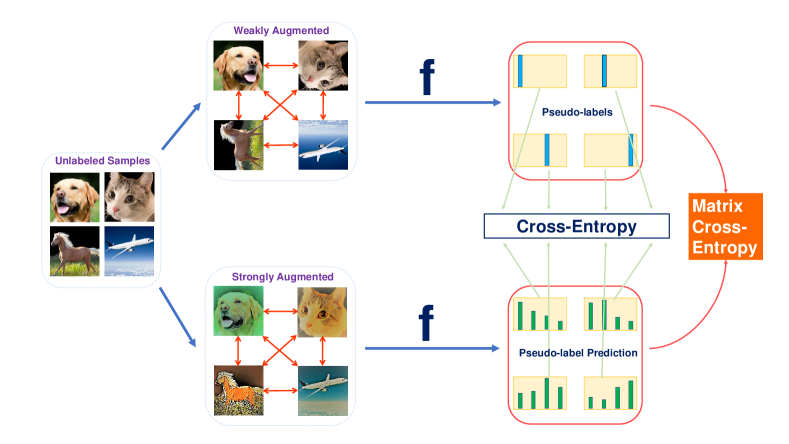
Figure 1: An illustration of the RelationMatch method for Semi-supervised Learning.

In this paper, we propose to additionally enforce the consistency between the in-batch relationships of weak/strong augmentations in each batch. See Figure 1. In the upper row, the four images are only weakly augmented, and assume that $f$ gives the correct pseudo-labels for them. For the strongly augmented images in the lower row, the existing algorithms only consider pairwise consistency using cross-entropy, which means the prediction of the strongly augmented dog shall be close to the one-hot vector for dog, and the strongly augmented cat shall be close to the one-hot vector for cat, etc. In addition to this regularization, we propose RelationMatch, which uses the matrix cross-entropy loss (MCE) to capture the in-batch relationships between the images. Therefore, we hope $f$ believes the relationship between the weakly augmented dog and weakly augmented cat, shall be close to the relationship between the strongly augmented dog and strongly augmented cat:

$$\mathrm{Relation}(\text{WeaklyAug dog},\text{WeaklyAug cat})\approx\mathrm{Relation}(\text{StronglyAug dog},\text{StronglyAug cat})$$

Formally, we represent each image $x$ with the prediction vector $f(x)\in\mathbb{R}^{k}$. We use the inner products between images to represent their relationship. Notice that such relationships are always computed for the same type of augmentations, e.g., between weakly augmented dog and weakly augmented cat, but never between weakly augmented dog and strongly augmented cat. For each mini-batch of samples of $b$ images, consider their weak (or strong) augmentations. Using $f$ to represent these images, we get a relationship matrix $A\in\mathbb{R}^{b\times k}$, where each row of $A$ represents the prediction vector of an image. By computing $R(A)\triangleq AA^{\top}$, we get a $b\times b$ matrix, which stores all the relationships between any two images in the batch. Notice that we will compute different relationship matrices for weak/strong augmentations, denoted as $R(A^{w})$ and $R(A^{s})$, respectively.

To define the loss for matching $R(A^{w})$ and $R(A^{s})$, we adopt two distinct theoretical perspectives to generalize the cross-entropy loss of vectors to MCE, deriving from both matrix analysis and information geometry. Intriguingly, our MCE loss emerges as the natural choice from both aspects and possesses numerous desirable properties. In our experiments, we observe RelationMatch incurs a significant performance uplift for STL-10, and consistent improvements for CIFAR-10 as well. Interestingly, we find that it also proves effective for supervised learning scenarios.

Our contributions can be summarized in three folds:

• We introduce RelationMatch, a new semi-supervised learning algorithm that exploits the in-batch relationship consistency during training.

• We propose the matrix cross-entropy (MCE) loss through two different theoretical perspectives, which enjoyes many nice properties.

• We test RelationMatch on CIFAR-10, CIFAR-100 and STL-10, which consistently outperforms the state-of-the-art semi-supervised learning methods, especially for the STL-10 40 labels setting, outperform the well-known method Flexmatch (Zhang et al., 2021) by 15.21%. It also has consistent improvements for supervised learning scenarios.

2 Related Work

Semi-supervised learning aims to improve model performance by leveraging substantial amounts of unlabeled data and has garnered significant interest in recent years (Chen et al., 2020b; Assran et al., 2021; Wang et al., 2021). The invariance principle forms the basis for most effective semi-supervised algorithms. At its core, this principle asserts that two semantically similar images should produce similar representations when processed by the same backbone.

Consistency regularization

A prevalent method for implementing the invariance principle is through consistency regularization, initially introduced in the $\Pi$-Model (Rasmus et al., 2015b). This technique has been widely adopted in later research (Tarvainen & Valpola, 2017; Laine & Aila, 2016; Berthelot et al., 2019b). Consistency regularization generally involves generating pseudo-labels and applying suitable data augmentation (Tschannen et al., 2019; Berthelot et al., 2019b; Xie et al., 2020; Sohn et al., 2020; Gong et al., 2021). Pseudo-labels can be created for unlabeled data and used in subsequent training iterations (Lee et al., 2013). The conventional approach employs an entropy minimization objective to fit the generated pseudo-labels (Rasmus et al., 2015b; Laine & Aila, 2016; Tarvainen & Valpola, 2017). Specifically, it aligns the predicted pseudo-labels of two distorted images (typically obtained through data augmentation). Furthermore, several studies have investigated the generation of efficient and valuable pseudo-labels that consider numerous practical factors (Hu et al., 2021; Nassar et al., 2021; Xu et al., 2021; Zhang et al., 2021; Li et al., 2022; Wang et al., 2022b). Consistency regularization has proven to be a simple and effective approach, serving as a foundational component in many state-of-the-art semi-supervised learning algorithms(Sohn et al., 2020; Zhang et al., 2021).

Improving pseudo-label quality

Existing discussions on consistency regularization mainly center around enhancing the quality of pseudo-labels. For instance, SimPLE (Hu et al., 2021) introduces paired loss, which minimizes the statistical distance between confident and similar pseudo-labels. Dash (Xu et al., 2021) and FlexMatch (Zhang et al., 2021) propose dynamic and adaptive pseudo-label filtering, which is more suited for the training process. CoMatch (Li et al., 2021) suggests incorporating contrastive learning into the semi-supervised learning framework, jointly learning two representations of the training data. SemCo (Nassar et al., 2021) accounts for external label semantics to prevent pseudo-label quality degradation for visually similar classes in a co-training approach. FreeMatch (Wang et al., 2022c) recommends a self-adaptive adjustment of the confidence threshold, taking into consideration the learning status of the models. MaxMatch (Li et al., 2022) presents a worst-case consistency regularization technique that minimizes the largest inconsistency between an original unlabeled sample and its multiple augmented versions, with theoretical guarantees. NP-Match (Wang et al., 2022a) employs neural processes to enhance pseudo-label quality. SEAL (Tan et al., 2023) proposes simultaneously learning a data-driven label hierarchy and performing semi-supervised learning. SoftMatch (Chen et al., 2023) identifies the inherent quantity-quality trade-off issue of pseudo-labels with thresholding, which may hinder learning, and proposes using a truncated Gaussian function to weight samples based on their confidence.

In this study, we pursue an alternative approach other than improving pseudo-label quality. Our method, Matrix Cross-Entropy (MCE), serves as a universal generalization of classical cross-entropy and can be easily integrated into any supervised and semi-supervised methods with minimal computational overhead.

3 RelationMatch: Matrix Cross-Entropy for Semi-supervised Learning

3.1 Warm-up example

To better illustrate how we capture the relationships for both types of augmentations, we first present a simple warm-up example. Consider $b=4,k=3$, and three of the four images belong to the first class, while the second one belongs to the last class. Assume $f$ gets all the pseudo labels correctly for the weak augmentations, which means $R(A^{w})$ is defined as (recall $R(A)\triangleq AA^{\top}$):

$$R\left(\begin{bmatrix}1&0&0\\ 0&0&1\\ 1&0&0\\ 1&0&0\end{bmatrix}\right)=\begin{bmatrix}1&0&1&1\\ 0&1&0&0\\ 1&0&1&1\\ 1&0&1&1\end{bmatrix}$$ (1)

Since the pseudo labels for weak augmentations are always one-hot vectors, $R(A^{w})$ is well structured. Specifically, for rows that are same in $A^{w}$, they are also same in $R(A^{w})$, with value representing the corresponding row indices. In other words, $R(A^{w})$ represents $k$ distinct clusters of one-hot vectors in the mini-batch.

If $f$ can generate exactly the same prediction matrix $A^{s}$ for the strongly augmented images, our algorithm will not incur any additional loss compared with the previous cross-entropy based algorithms. However, $A^{s}$ and $A^{w}$ are generally different, where our algorithm becomes useful. For example, given a pair of prediction vectors $(p,q)$, if we know $p=(1,0,0)$, then cross-entropy loss is simply $p_{i}\log q_{i}=\log q_{i}$. Therefore, we will get the same loss for $q=(0.5,0.5,0)$, $q=(0.5,0.25,0.25)$, or $q=(0.5,0,0.5)$. Consider the following two possible cases of $R(A^{s})$ generated by $f$ during training:

$$R\left(\begin{bmatrix}0.5&0.5&0\\ 0&0&1\\ 0.5&0.5&0\\ 0.5&0.5&0\end{bmatrix}\right)=\begin{bmatrix}0.5&0&0.5&0.5\\ 0&1&0&0\\ 0.5&0&0.5&0.5\\ 0.5&0&0.5&0.5\end{bmatrix}$$

$$R\left(\begin{bmatrix}0.5&0.5&0\\ 0&0&1\\ 0.5&0.25&0.25\\ 0.5&0&0.5\end{bmatrix}\right)=\begin{bmatrix}0.5&0&0.375&0.25\\ 0&1&0.25&0.5\\ 0.375&0.25&0.375&0.375\\ 0.25&0.5&0.375&0.5\end{bmatrix}$$

If we only use cross-entropy loss, these two cases will give us the same gradient information. However, by considering the in-batch relationships, it becomes clear that these two cases are different: the first case always makes mistakes on the second class, while the second case makes relatively random mistakes. Therefore, by comparing $R(A^{s})$ with $R(A^{w})$ defined in Eqn. (1), we can get additional training signals. In our example, the first case will not give additional gradient information for the second row (and the second column due to symmetry), but the second case will.

3.2 Matrix cross-entropy

Since $R(A)\triangleq AA^{\top}$, we know that both $R(A^{w})$ and $R(A^{s})$ are positive semi-definite. We use the matrix cross-entropy (MCE) loss for measuring their distance, defined below.

Definition 3.1 (Matrix cross-entropy for positive semi-definite matrices).

Let $\bm{P},\bm{Q}$ be positive semi-definite matrices. The matrix cross-entropy of $\bm{P}$ with respect to $\bm{Q}$ is defined as:

$$\mathrm{MCE}(\bm{P},\bm{Q})\triangleq\operatorname{tr}(-\bm{P}\log\bm{Q}+\bm{Q}).$$ (2)

Here $\operatorname{tr}$ denotes the matrix trace, $\log$ denotes the principal matrix logarithm defined in Appendix A.

At the first glance, the MCE loss looks like a complicated and random expression. However, as we will discuss in Section 5, it can be naturally derived from both matrix analysis (Section 5.1) and information geometry (Section 5.2). Moreover, it has a nice interpretation from matrix eigen-decomposition (Appendix A.3). In Section 6, we further demonstrate that the standard cross-entropy loss can be seen as a special case of MCE, as well as some of its nice properties.

3.3 RelationMatch: Applying MCE for Semi-supervised Learning

We consider a general scheme (Lee et al., 2013; Gong et al., 2021) that unifies many prior semi-supervised algorithms (including FixMatch and FlexMatch):

$$\theta_{n+1}\leftarrow\underset{\theta}{\arg\min}\left\{\mathcal{L}_{s}\left(\theta\right)+\mu_{u}\mathcal{L}_{u}\left(\theta;\theta_{n}\right)\right\},$$ (3)

where $\theta_{n}$ denotes the model parameters at the $n$-th iteration, $\mathcal{L}_{s}(\theta)$ is a supervised loss. The unsupervised loss term $\mathcal{L}_{u}(\theta;\theta_{n})$ acts as a consistency regularization (based on the $n$-th step backbone) that operates on the unlabeled data, and $\mu_{u}$ is a loss balancing hyperparameter.

During training, we always have access to some labeled data and unlabeled data. Assume there are $b_{s}$ labeled images and $b_{u}$ unlabeled images. For labeled data, the loss is the classical cross-entropy loss combined with matrix cross-entropy loss. For those $b_{u}^{\prime}$ unlabeled data that are pseudo-labeled, we also have CE combined with MCE (where we use pseudo labels provided by weakly augmented images, denoted as $\tilde{Y}$). In summary, we have:

$$\mathcal{L}_{\text{RelationMatch}}(Y,X)=\mathcal{L}_{s}(Y_{s},X_{s})+\mu_{u}\mathcal{L}_{u}(X_{u})$$ (4)

$$=\sum_{i=1}^{b_{s}}\operatorname{CE}(y_{i},x_{i})+\operatorname{MCE}(Y_{s},X_{s})+\mu_{u}\left(\sum_{i=1}^{b_{u}}\operatorname{CE}(\tilde{y}_{i},\tilde{x}_{i})+\operatorname{MCE}(\tilde{Y}_{s},\tilde{X}_{s})\right)$$

We remark that Section 5 and Section 6 are purely theoretical and require the readers to have very strong mathematical background. Skipping these two sections does not affect understanding and implementing our RelationMatch method. Therefore, we choose to present our experimental results first, and curious readers may read Section 5 and Section 6 afterwards.

4 Experiments

4.1 Dataset

CIFAR-10/100

CIFAR-10 (Krizhevsky et al., 2009) is a widely-used classical image classification dataset. It consists of 60,000 images from 10 different classes, with 50,000 designated for training and 10,000 for testing. Each class has 5,000 training and 1,000 test images. All images in CIFAR-10 are $3\times 32\times 32$ pixels. CIFAR-100 (Krizhevsky et al., 2009) is similar to CIFAR-10 but contains 100 classes, each with 600 images, 500 for training and 100 for testing.

STL-10

STL-10 (Coates et al., 2011) is a semi-supervised benchmark dataset derived from ImageNet (Deng et al., 2009). STL-10 contains 10 labeled classes, providing 500 training images and 800 test images per class, as well as 100,000 unlabeled images for semi-supervised learning. Some unlabeled images originate from classes other than the 10 labeled ones. All images in STL-10 are $3\times 96\times 96$ color images.

4.2 Experiment Details

Implementation

Our algorithm is implemented using TorchSSL (Zhang et al., 2021), the official implementation of FlexMatch (Zhang et al., 2021), which is also a PyTorch-based toolbox for semi-supervised learning (Paszke et al., 2019). We modify the code so that when TorchSSL calculates the unsupervised cross-entropy loss, we concurrently compute the MCE loss and add it to the final loss (for more on implementation details, please refer to Appendix B).

Hyperparameters

For a fair comparison, we use the same hyperparameters as FixMatch (Sohn et al., 2020). We employ an SGD optimizer with 0.9 momentum and $5\times 10^{-4}$ weight decay. The learning rate is scheduled using a cosine scheduler and initialized at $0.03$. The batch size is set to 64, and the ratio of unlabeled data to labeled data is 7 during training. The threshold, $\tau$, is set to 0.95. For CIFAR-10, we use WideResNet-28-2 (Zagoruyko & Komodakis, 2016) as the backbone, and WideResNetVar-28-2 for STL-10. We train each model for $2^{20}$ training steps, with each step sampling an equal number of labeled images from all classes. To stabilize numerical calculations, we add $\lambda\mathbf{I}$ regularization to the matrices $\mathbf{P}$ and $\mathbf{Q}$ in MCE.

Baselines

We consider prior semi-supervised learning methods similar to FixMatch, including $\Pi$-Model, Pseudo-Label (Lee et al., 2013), VAT (Miyato et al., 2018), MeanTeacher (Tarvainen & Valpola, 2017), MixMatch (Berthelot et al., 2019b), ReMixMatch (Berthelot et al., 2019a), UDA (Xie et al., 2020), Dash (Xu et al., 2021), MPL (Pham et al., 2021), FixMatch (Sohn et al., 2020), and FlexMatch (Zhang et al., 2021). Most baseline results are directly obtained from TorchSSL. For recent and future works on improving pseudo-label quality such as CPL introduced in Flexmatch, our method can be easily incorporated with them.

4.3 Experimental results on supervised learning

First, we report our evaluation results using WideResNet-28-2, ResNet18, and ResNet50 in the fully-supervised setting. We train the models for 200 epochs using a cosine learning rate scheduler with a batch size of 64, and the results are shown in Table 1.

Label smoothing was first introduced by Szegedy et al. (2016) and has been widely used to improve supervised learning generalization across various tasks, such as image classification, language translation, and speech recognition. However, Müller et al. (2019) argue that label smoothing may erase information (using mutual information measurement) and lead to inferior performance when applied to knowledge distillation. Interestingly, Lemmas A.9 demonstrates that MCE retains one-hot properties without losing information.

Table 1: Accuracy results of our method compared to baselines (including label smoothing) under supervised settings. WRN means WideResNet.

Dataset	CIFAR-10
# Backbone	WRN-28-2	ResNet18	ResNet50
only cross-entropy	94.45$\pm$0.19	95.08$\pm$0.09	95.32$\pm$0.18
w/ label-smoothing	94.72$\pm$0.05	95.25$\pm$0.13	95.10$\pm$0.32
w/ matrix cross-entropy	94.79$\pm$0.05	95.31$\pm$0.08	95.46$\pm$0.16

4.4 Experimental results on semi-supervised learning

We report our evaluation results for different models on benchmark datasets in Table 2.

Better performance

It is evident that RelationMatch outperforms the baselines in most cases, and significantly improves over the baselines for the STL-10 dataset with 40 labels. It is important to note that in both CIFAR-10 cases, Flexmatch has already achieved at least 95% accuracy, making it difficult for RelationMatch with CPL (Zhang et al., 2021) to demonstrate significant improvement. However, in the case of STL-10, we observe a 15.21% accuracy gain with 40 labels.

Universal generalization of cross-entropy with minimal computation overhead

Matrix cross-entropy can be incorporated wherever cross-entropy is used, and the computational overhead is less than 2%. For example, in the CIFAR-10 experiments using NVIDIA A10, the runtime per epoch is 31.5s for the original method and 32.1s when using MCE.

Table 2: Error rates (100% - accuracy) on CIFAR-10, CIFAR-100, and STL-10 dataset for state-of-the-art methods for semi-supervised learning, bold means the best, underline means the second.

Dataset	CIFAR-10			CIFAR-100			STL-10
# Label	40	250	4000	400	2500	10000	40	250	1000
$\Pi$ Model (Rasmus et al., 2015a)	74.34$\pm$1.76	46.24$\pm$1.29	13.13$\pm$0.59	86.96$\pm$0.80	58.80$\pm$0.66	36.65$\pm$0.00	74.31$\pm$0.85	55.13$\pm$1.50	32.78$\pm$0.40
Pseudo Label (Lee et al., 2013)	74.61$\pm$0.26	46.49$\pm$2.20	15.08$\pm$0.19	87.45$\pm$0.85	57.74$\pm$0.28	36.55$\pm$0.24	74.68$\pm$0.99	55.45$\pm$2.43	32.64$\pm$0.71
VAT (Miyato et al., 2018)	74.66$\pm$2.12	41.03$\pm$1.79	10.51$\pm$0.12	85.20$\pm$1.40	46.84$\pm$0.79	32.14$\pm$0.19	74.74$\pm$0.38	56.42$\pm$1.97	37.95$\pm$1.12
MeanTeacher (Tarvainen & Valpola, 2017)	70.09$\pm$1.60	37.46$\pm$3.30	8.10$\pm$0.21	81.11$\pm$1.44	45.17$\pm$1.06	31.75$\pm$0.23	71.72$\pm$1.45	56.49$\pm$2.75	33.90$\pm$1.37
MixMatch (Berthelot et al., 2019b)	36.19$\pm$6.48	13.63$\pm$0.59	6.66$\pm$0.26	67.59$\pm$0.66	39.76$\pm$0.48	27.78$\pm$0.29	54.93$\pm$0.96	34.52$\pm$0.32	21.70$\pm$0.68
ReMixMatch (Berthelot et al., 2019a)	9.88$\pm$1.03	6.30$\pm$0.05	4.84$\pm$0.01	42.75$\pm$1.05	26.03$\pm$0.35	20.02$\pm$0.27	32.12$\pm$6.24	12.49$\pm$1.28	6.74$\pm$0.14
UDA (Xie et al., 2020)	10.62$\pm$3.75	5.16$\pm$0.06	4.29$\pm$0.07	46.39$\pm$1.59	27.73$\pm$0.21	22.49$\pm$0.23	37.42$\pm$8.44	9.72$\pm$1.15	6.64$\pm$0.17
Dash (Xu et al., 2021)	8.93$\pm$3.11	5.16$\pm$0.23	4.36$\pm$0.11	44.82$\pm$0.96	27.15$\pm$0.22	21.88$\pm$0.07	34.52$\pm$4.30	-	6.39$\pm$0.56
MPL (Pham et al., 2021)	6.93$\pm$0.17	5.76$\pm$0.24	4.55$\pm$0.04	46.26$\pm$1.84	27.71$\pm$0.19	21.74$\pm$0.09	35.76$\pm$4.83	9.90$\pm$0.96	6.66$\pm$0.00
FixMatch (Sohn et al., 2020)	7.47$\pm$0.28	5.07$\pm$0.05	4.21$\pm$0.08	46.42$\pm$0.82	28.03$\pm$0.16	22.20$\pm$0.12	35.97$\pm$4.14	9.81$\pm$1.04	6.25$\pm$0.33
FlexMatch (Zhang et al., 2021)	4.97$\pm$0.06	4.98$\pm$0.09	4.19$\pm$0.01	39.94$\pm$1.62	26.49$\pm$0.20	21.90$\pm$0.15	29.15$\pm$4.16	8.23$\pm$0.39	5.77$\pm$0.18
RelationMatch	6.87$\pm$0.12	4.85$\pm$0.04	4.22$\pm$0.06	45.79$\pm$0.59	27.90$\pm$0.15	22.18$\pm$0.13	33.42$\pm$3.92	9.55$\pm$0.87	6.08$\pm$0.29
RelationMatch (w/ CPL)	4.96$\pm$0.05	4.88$\pm$0.05	4.17$\pm$0.04	39.89$\pm$1.43	26.48$\pm$0.18	21.88$\pm$0.16	13.94$\pm$3.76	8.16$\pm$0.34	5.68$\pm$0.19
Fully-Supervised	4.62$\pm$0.05			19.30$\pm$0.09			-
Fully-Supervised w/ MCE	4.38$\pm$0.07			19.25$\pm$0.10			-

5 Matrix Cross-Entropy: Derivations and Interpretations

In this section, we present different derivations of MCE, from matrix analysis and information geometry. Afterward, we also give an interpretation of MCE based on matrix eigen-decomposition in Appendix A.3.

5.1 Matrix analysis perspective

Definition 5.1 (Density matrix on $\mathbb{R}^{n\times n}$).

A matrix $\mathbf{A}\in\mathbb{R}^{n\times n}$ is called a density matrix if it is symmetric, positive semi-definite, and has a trace equal to $1$.

We can view the density matrix as a natural generalization of classical probability theory. For any symmetric positive semi-definite matrix, its eigenvalues are non-negative real numbers, similar to probabilities being non-negative. Additionally, the trace of a matrix $A$ equals the sum of its eigenvalues, and unit trace constraints coincide with probability constraints that should sum up to 1.

As density matrices serve the role of probability in matrix theory, we first define some matrix functions based on their probability counterpart. We introduce the definition of matrix logarithm for ease of exposition; it is a matrix version of the classical logarithm function.

Definition 5.2 (Matrix logarithm).

The exponential of a matrix $\mathbf{A}$ is defined by

$$e^{\mathbf{A}}:=\sum_{i=0}^{\infty}\frac{\mathbf{A}^{n}}{n!}$$

Matrix $\mathbf{B}$ is called the matrix logarithm of the matrix $\mathbf{A}$ if it satisfies $e^{\mathbf{A}}=\mathbf{B}$.

There may be infinitely many possible matrix logarithms for a given $\mathbf{A}$, but the principal matrix logarithm provides a unique definition of the matrix logarithm for the density matrix $\mathbf{A}$ (refer to Theorem A.1 in Appendix A).

Proposition 5.3.

For the density matrix $\mathbf{A}\in\mathbb{R}^{n\times n}$, suppose it has spectral decomposition $\mathbf{A}=\mathbf{U}\mathbf{\Lambda}\mathbf{U}^{\top}$, then its (principal) logarithm can be expressed as:

$$\log\mathbf{A}=\mathbf{U}\operatorname{diag}(\log(\lambda_{i}))\mathbf{U}^{\top}.$$

Here we define $0\log(0)\triangleq 0$, and we define $\operatorname{diag}$ operator in Appendix A.

Lemma 5.4.

For density matrix $\mathbf{A}$, its von Neumann entropy equals to Shannon entropy defined on its eigenvalues:

$$-\operatorname{tr}(\mathbf{A}\log\mathbf{A})=-\sum_{i}\lambda_{i}\log(\lambda_{i}).$$

The main reason for introducing classical cross-entropy is for the simplicity of its optimization compared to classical KL divergence (relative entropy). Similarly, we introduce the matrix cross-entropy, which can be seen as a reduced form of matrix (von Neumann) divergence. Inspired by classical cross-entropy:

$$H(p,q)=H(p)+D_{\text{KL}}(p\|q)$$

For density matrices $\bm{P}$ and $\bm{Q}$, we define the density matrix cross-entropy as

$$\operatorname{MCE}_{\text{density-matrix}}(\bm{P},\bm{Q})\triangleq H(\bm{P})+\mathrm{MRE}(\bm{P},\bm{Q}),$$ (5)

where $H(\bm{P})$ is the matrix (von Neumann) entropy, and the matrix relative entropy is defined as follows (For more properties of matrix relative entropy, please see Appendix A.2).

Definition 5.5 (Matrix relative entropy for density matrices).

Let $\mathbf{P},\mathbf{Q}\in\mathbb{R}^{n\times n}$ be density matrices. The matrix relative entropy of $\mathbf{P}$ with respect to $\mathbf{Q}$ is defined as

$$\mathrm{MRE}(\mathbf{P},\mathbf{Q})\triangleq\operatorname{tr}(\mathbf{P}\log\mathbf{P}-\mathbf{P}\log\mathbf{Q}).$$ (6)

5.2 Information geometry perspective

Information geometry provides a viewpoint for extending matrix cross-entropy from the density matrix with unit trace to general positive semi-definite matrices. Amari (2014) demonstrates that the Bregman divergence, determined by a convex function $\phi$, can induce a dually flat structure on the positive semi-definite matrix cone. The matrix Bregman divergence is defined as follows:

$$\operatorname{D}[\mathbf{P}:\mathbf{Q}]=\phi(\mathbf{P})-\phi(\mathbf{Q})-\nabla\phi(\mathbf{P})\cdot(\mathbf{P}-\mathbf{Q}).$$

If we choose $\phi(\mathbf{P})$ as the negative matrix entropy, we obtain:

$$\operatorname{MD}[\mathbf{P}:\mathbf{Q}]=\operatorname{tr}(\mathbf{P}\log\mathbf{P}-\mathbf{P}\log\mathbf{Q}-\mathbf{P}+\mathbf{Q}).$$ (7)

As $\bm{P}$ usually be seen as a reference term that can hold fixed, taking the Bregman divergence with variable $\bm{Q}$ gives MCE in Definition 3.1. Note that MCE is simply $H(\bm{P},\bm{Q})$ with an added penalty term $\operatorname{tr}(\mathbf{Q})$. It can be seen as the Lagrange multiplier method for the $\operatorname{tr}(\mathbf{Q})=1$ density matrix constraint. Thus, our proposed MCE benefits from both density matrix and information geometry theories.

Theorem 5.6 (Projection Theorem (Amari, 2014)).

Given a smooth submanifold, $S$, let $\mathbf{P}_{S}$ be the minimizer of divergence from $\mathbf{P}$ to $\mathbf{S}$,

$$\mathbf{P}_{S}=\min_{\mathbf{Q}\in S}\operatorname{D}[\mathbf{P}:\mathbf{Q}].$$

Then, $P_{S}$ is the $\bm{\eta}$-geodesic projection of $\mathbf{P}$ to $\mathbf{S}$, that is the $\bm{\eta}$-geodesic connecting $\mathbf{P}$ and $\mathbf{P}_{S}$ is orthogonal to $\mathbf{S}$.

The projection theorem gives the minimization property for MCE:

Proposition 5.7 (Minimization property).

$$\operatorname{argmin}_{\mathbf{Q}\succ 0}\mathrm{MCE}(\mathbf{P},\mathbf{Q})=\mathbf{P}.$$ (8)

Proof.

Use Theorem 5.6. ∎

6 Matrix Cross-Entropy: Properties

6.1 What is the scalar cross-entropy?

We show below that the traditional scalar cross-entropy loss is a special case of our MCE loss.

Suppose we have $b$ pairs of $k$ dimensional probability vectors pairs $\{(\mu_{i},\nu_{i})\}^{b}_{i=1}$. Denote $\mu_{i}=(\mu^{(1)}_{i},\cdots,\mu^{(k)}_{i})$ and $\nu_{i}=(\nu^{(1)}_{i},\cdots,\nu^{(k)}_{i})$.

Then from the definition of scalar cross-entropy and MCE loss, we shall have $H(\mu_{i},\nu_{i})=-\sum^{k}_{j=1}\mu^{(j)}_{i}\log\nu^{(j)}_{i}=-\operatorname{tr}(\operatorname{diag}(\mu_{i})\log\operatorname{diag}(\nu_{i}))$.

The above shows one of the important concerns of density matrices, i.e. it cares about the spectral.

When the labels are represented by one hot encoding, there exists another formulation involves the correlation. It cares only about self-correlation and neglects cross-correlation. Let $\mathbf{M}\in\mathbb{R}^{k\times b}$ be concatenations of one-hot distributions $\mu_{i}$, with $i$-th column as $\mu_{i}$. Let $\mathbf{N}\in\mathbb{R}^{k\times b}$ be concatenations of distributions $\nu_{i}$, with $i$-th column as $\nu_{i}$.

Define

$$\mathbf{P}=\frac{1}{b}\mathbf{I}_{b},\mathbf{Q}=\mathbf{I}_{b}\circ(\mathbf{M}^{\top}\mathbf{N}),$$

where $\circ$ is the Hardmard product. Then $\operatorname{tr}(-\mathbf{P}\log\mathbf{Q})$ gives the (averaged) cross-entropy loss.

6.2 Properties of MCE

In this subsection, we demonstrate a few nice properties of MCE, indicating that it is an ideal candidate for being a loss function.

Lemma 6.1.

Let $\mathbf{A}\in\mathbb{R}^{m\times n}\setminus\{\mathbf{0}\}$ so that $\operatorname{tr}(\mathbf{A}\mathbf{A}^{\top})=\operatorname{tr}(\mathbf{A}^{\top}\mathbf{A})>0$. then $\frac{\mathbf{A}\mathbf{A}^{\top}}{\operatorname{tr}(\mathbf{A}\mathbf{A}^{\top})}$ and $\frac{\mathbf{A}^{\top}\mathbf{A}}{\operatorname{tr}(\mathbf{A}^{\top}\mathbf{A})}$ are density matrices.

Proof.

Use the singular value decomposition of $\mathbf{A}$. ∎

From Lemma 6.1, we know that during training, relation matrix $R(A^{w})$ and $R(A^{s})$ always satisfy the density matrix constraints, which give us many satisfying properties as below.

Proposition 6.2 (Linearity).

$$\mathrm{MCE}\left(\sum_{i}a_{i}\bm{P}_{i},\bm{Q}\right)=\sum_{i}a_{i}\mathrm{MCE}(\bm{P}_{i},\bm{Q}).$$

Proposition 6.3 (Convexity).

For any convex combination $b_{j}$, we have

$$\mathrm{MCE}\left(\bm{P},\sum_{j}b_{j}\bm{Q}_{j}\right)\leq\sum_{j}b_{j}\mathrm{MCE}\left(\bm{P},\bm{Q}_{j}\right).$$

Proof.

From the joint convexity of matrix relative entropy, which is stated in Proposition A.8. ∎

Kornblith et al. (2019) suggests that a good measuring similarity of neural network representations should be invariance to orthogonal (unitary) transformation.

Lemma 6.4.

Suppose $\mathbf{A}\in\mathbb{R}^{n\times n}$ is a density matrix, $\mathbf{U}\in\mathbb{R}^{m\times n}$ is a unitary matrix, then $\mathbf{U}\mathbf{A}\mathbf{U}^{\top}$ is a density matrix.

Proposition 6.5 (Invariance property).

$\mathrm{MCE}(\mathbf{P},\mathbf{Q})$ is invariant under simultaneous unitary transformation on both $\mathbf{P}$ and $\mathbf{Q}$ :

$$\mathrm{MCE}(\mathbf{P},\mathbf{Q})=\mathrm{MCE}\left(\mathbf{U}\mathbf{P}\mathbf{U}^{\top},\mathbf{U}\mathbf{Q}\mathbf{U}^{\top}\right)$$

Proof.

Use Lemma 6.4 and spectral decomposition of $\mathbf{P}$ and $\mathbf{Q}$. ∎

The following lower bounded property shows the advantage of MCE being a loss function, such that we can directly opt for off-the-shelf (stochastic) gradient descent optimizers.

Proposition 6.6 (Lower bounded property).

$\mathrm{MCE}(\mathbf{P},\mathbf{Q})$ has the following lower bound when $\mathbf{P}$ is a density matrix:

$$\mathrm{MCE}(\mathbf{P},\mathbf{Q})\geq-\log\operatorname{tr}(\mathbf{P}\mathbf{Q})+\operatorname{tr}(\mathbf{Q})$$

Proof.

Use spectral decomposition of $\mathbf{P}$ and $\mathbf{Q}$ and trace inequalities. ∎

7 Conclusion

In this paper, we pursue an alternative approach other than improving pseudo-label quality, introducing RelationMatch, a new semi-supervised learning algorithm that exploits the in-batch relationship consistency during training. To capture the in-batch relationships, we introduce a novel loss function called matrix cross-entropy (MCE). We derive this loss function from two perspectives: matrix analysis and information geometry. We also explore its theoretical properties and experimentally evaluate its effectiveness on several vision datasets. Our experiments demonstrate that MCE consistently outperforms state-of-the-art methods and offers a universal generalization of cross-entropy with minimal computational overhead. This work not only contributes to the understanding of semi-supervised learning but also provides a promising direction for incorporating the MCE loss in future research.

Acknowledgments

This work is supported by the Ministry of Science and Technology of the People’s Republic of China, the 2030 Innovation Megaprojects “Program on New Generation Artificial Intelligence” (Grant No. 2021AAA0150000).

Author Contributions

Yifan Zhang proposed the matrix cross-entropy loss, as well as the derivations from the density matrix and information geometry perspectives. Jingqin Yang implemented most of the experiments and wrote the experimental section. Zhiquan Tan used trace normalization to show the relationship between MRE and MCE. He also provided the PCA viewpoint of MCE, and proved most of the theorems. Yang Yuan wrote the introduction, and provided the warm-up example.

Appendix A More on Proofs

Theorem A.1 (Principal matrix logarithm (Higham, 2008)).

Let $\mathbf{A}\in\mathbb{C}^{n\times n}$ have no eigenvalues on $\mathbb{R}^{-}$. There is a unique logarithm $\mathbf{X}$ of $\mathbf{A}$ of whose all eigenvalues lie in the strip $\{z$ : $-\pi<\operatorname{Im}(z)<\pi\}$. We refer to $\mathbf{X}$ as the principal logarithm of $\mathbf{A}$ and write $\mathbf{X}=\log(\mathbf{A})$. If $\mathbf{A}$ is real then its principal logarithm is real.

Not otherwise specified, we use the principal matrix logarithm as default in the following sections.

A.1 Density matrices

Here we give more discussions on density matrices. One can easily convert a density matrix into a probability distribution by the following proposition.

Proposition A.2.

Suppose we have $X=\{x_{i}|i=1,2,\cdots,n\}$ as an othornormal basis for $\mathbb{R}^{n}$, then any density matrix $\mathbf{A}\in\mathbb{R}^{n\times n}$ induce a probability distribution on $X$: $P(x=x_{i})=x_{i}^{\top}\mathbf{A}x_{i}$.

For ease of exposition, we introduce the diag operator from $\mathbb{R}^{n}$ to $\mathbb{R}^{n\times n}$. It is defined as:

$$\operatorname{diag}(a):=\begin{pmatrix}{}a_{1}&0&\cdots&0\\ 0&a_{2}&\cdots&0\\ \vdots&\vdots&\ddots&0\\ 0&0&\cdots&a_{n}\\ \end{pmatrix}.$$

Given a probability distribution, we can easily convert it to a density matrix as well, either as a diagonal matrix in Proposition A.3 or as the orthogonal projection in Proposition A.4.

Proposition A.3.

For any probability distribution $\sum_{i}P(x=x_{i})=1$, we can construct a diagonal density matrix as follow:

$$\mathbf{A}_{\text{diag }}=\left[\begin{array}[]{llll}P(x=x_{1})&&&\\ &P(x=x_{2})&&\\ &&\ddots&\\ &&&P(x=x_{n})\end{array}\right]$$

Proposition A.4.

Suppose we have $X=\{x_{i}|i=1,2,\cdots,n\}$ as an orthonormal basis for $\mathbb{R}^{n}$, for any probability distribution $\sum_{i}P(x=x_{i})=1$, we can construct an orthogonal projection density matrix as follow:

$$\psi=\sum_{i}\sqrt{P(x=x_{i})}x_{i}$$

$$\mathbf{A}_{\text{op}}=\psi\psi^{\top}=\sum_{i,j}\sqrt{P(x_{i})P(x_{j})}x_{i}x_{j}^{\top}$$

One can verify that $P(x=x_{i})=x_{i}^{\top}\mathbf{A}_{\text{diag}}x_{i}=x_{i}^{\top}\mathbf{A}_{\text{op}}x_{i}$. However, $\mathbf{A}_{\text{diag}}$ is mixed state, while $\mathbf{A}_{\text{op}}$ is pure state, according to the definition below. This is because $\mathbf{A}_{\text{diag}}$ has maximal rank while $\mathbf{A}_{\text{op}}$ has rank $1$.

Definition A.5 (Pure state and mixed state).

A density matrix $A$ is called a pure state if its rank equals to $1$ and is called a mixed state otherwise.

Interestingly, one can define the following entropy which can be seen as the generalization of entropy to the matrix form.

Definition A.6 (Matrix (von Neumman) entropy).

The mixedness of a density matrix can be quantified by matrix (von Neumann) entropy: $-\operatorname{tr}(\mathbf{A}\log\mathbf{A})$.

A.2 Matrix relative entropy for density matrices

In addition, we have matrix relative entropy for density matrices, satisfying non-negative and convex properties.

Proposition A.7.

The matrix relative entropy is non-negative:

$$\mathrm{MRE}(\mathbf{X};\mathbf{Y})\geq 0.$$

Equality holds if and only if $\mathbf{X}=\mathbf{Y}$.

Proof.

Use Klein’s inequality (Ruskai, 2002). ∎

The matrix relative entropy has nice convex properties proved by Lindblad (1974):

Proposition A.8 (Joint convexity (Lindblad, 1974)).

The matrix relative entropy is a jointly convex function:

$$\mathrm{MRE}\left(t\bm{X}_{1}+(1-t)\bm{X}_{2};t\bm{Y}_{1}+(1-t)\bm{Y}_{2}\right)\leq$$

$$\quad t\cdot\mathrm{MRE}\left(\bm{X}_{1};\bm{Y}_{1}\right)+(1-t)\cdot\mathrm{MRE}\left(\bm{X}_{2};\bm{Y}_{2}\right)$$

for $t\in[0,1]$, where $\bm{X}_{i}$ and $\bm{Y}_{i}$ are density matrices.

A.3 PCA-inspired interpretation

Given positive semi-definite matrices $\mathbf{P}$ and $\mathbf{Q}$, let their eigen decompositions be $\mathbf{P}=\mathbf{V}\mathbf{\Lambda}\mathbf{V}^{\top}$ and $\mathbf{Q}=\mathbf{U}\Theta\mathbf{U}^{\top}$. From the definition of the matrix logarithm, it is clear that $\log\mathbf{Q}=\mathbf{U}\log\mathbf{\Theta}\mathbf{U}^{\top}$. Next, we simplify the expression of $\operatorname{tr}(-\mathbf{P}\log\mathbf{Q})$ as follows:

$$\operatorname{tr}(-\mathbf{P}\log\mathbf{Q})= \operatorname{tr}(-\mathbf{V}\mathbf{\Lambda}\mathbf{V}^{\top}\mathbf{U}\log\mathbf{\Theta}\mathbf{U}^{\top})$$

$$= \operatorname{tr}(-\mathbf{\Lambda}\mathbf{V}^{\top}\mathbf{U}\log\mathbf{\Theta}\mathbf{U}^{\top}\mathbf{V})$$

$$= -\operatorname{tr}((\mathbf{\Lambda}\mathbf{V}^{\top}\mathbf{U})(\mathbf{V}^{\top}\mathbf{U}\log\mathbf{\Theta})^{\top})$$

Let the $i$-th column of $\mathbf{U}$ and $\mathbf{V}$ be $\mathbf{u}_{i}$ and $\mathbf{v}i$, respectively. Since the trace is related to the matrix inner product, we can derive that $\operatorname{tr}(-\mathbf{P}\log\mathbf{Q})=-\sum_{i,j}(\mathbf{v}_{i}^{\top}\mathbf{u}_{j})^{2}\lambda_{i}\log\theta_{j}$.

Ultimately, we obtain:

$$\operatorname{tr}(-\mathbf{P}\log\mathbf{Q}+\mathbf{Q})=-\sum_{i,j}\left(\mathbf{v}_{i}^{\top}\mathbf{u}_{j}\right)^{2}\lambda_{i}\log\theta_{j}+\sum_{j}\theta_{j}.$$ (9)

From this simplification, it is evident that $\sum_{j}\theta_{j}$ serves as a regularization term that penalizes $\theta_{j}$. The expression of the loss function also highlights the involvement of the correlation between eigenvectors and eigenvalues. When $\mathbf{P}$ and $\mathbf{Q}$ are covariance matrices or correlation matrices, their eigenvectors and eigenvalues are closely related to PCA.

A.4 Analysis the optimal point

What do we get if we achieves the optimal point of MCE loss? The next lemma gives a nice characterization.

Lemma A.9 (One-hot property).

Let $\mathbf{Z}_{1}\in\mathbb{R}^{b\times k}$ be the one hot probability encoding of a batch of images and $\mathbf{Z}_{2}\in\mathbb{R}^{b\times k}$ be the predicted probability distribution of a batch of images. If $\mathbf{Z}_{1}\mathbf{Z}_{1}^{\top}=\mathbf{Z}_{2}\mathbf{Z}_{2}^{\top}$, then every row of $\mathbf{Z}_{2}$ will be one hot and every two samples that belong to the same class in $\mathbf{Z}_{1}$ shall also belong to some same class in $\mathbf{Z}_{2}$.

Proof.

Note a vector lying on probability has its $l_{2}$ norm equal to $1$ iff it is one hot. By analyzing each diagonal entry of $\mathbf{Z}_{2}\mathbf{Z}_{2}^{\top}$, it is clear that each row of $\mathbf{Z}_{2}$ will be one hot. The rest of the argument is clear by analyzing each off-diagonal entry of $\mathbf{Z}^{\top}_{2}\mathbf{Z}_{2}$. ∎

Lemma A.9 says MCE describes the seconder order equivalence. That is, $\mathbf{Z}_{1}\mathbf{Z}_{1}^{\top}=\mathbf{Z}_{2}\mathbf{Z}_{2}^{\top}$ ensures that the rows of $\mathbf{Z}_{1}$ and $\mathbf{Z}_{2}$ have the same clustering pattern. However, it does not mean $\mathbf{Z}_{1}=\mathbf{Z}_{2}$. For example, consider the following $R(\mathbf{A})$, which gives the same output as Eqn. (1), but the input matrices are different.

$$R\left(\begin{bmatrix}0&0&1\\ 1&0&0\\ 0&0&1\\ 0&0&1\end{bmatrix}\right)=\begin{bmatrix}1&0&1&1\\ 0&1&0&0\\ 1&0&1&1\\ 1&0&1&1\end{bmatrix}$$

Interestingly, we can directly obtain the singular value decomposition for one-hot encoded data. Consider a (pseudo) labeled dataset ${(x_{i},y_{i})}^{B}_{i=1}$. Define the supporting (column) vectors $\mathbf{m}_{i}\in\mathbb{R}^{B}$ for class $i$ as follows:

$${m}_{i,j}=\left\{\begin{aligned} 1,&\text{ if }y_{j}=i.\\ 0,&\text{ otherwise. }\end{aligned}\right.$$

Denote $\mathbf{\hat{m}}_{i}=\frac{\mathbf{m}_{i}}{\lVert\mathbf{m}_{i}\rVert_{2}}$ and $\mathbf{e}_{i}\in\mathbb{R}^{K}$ as the $i$-th coordinate (column) vector. Then, $\sum^{K}_{i=1}\lVert\mathbf{m}_{i}\rVert_{2}\mathbf{e_{i}}\mathbf{\hat{m}}^{\top}_{i}$ yields the singular value decomposition for the one-hot encoded dataset. Since eigendecomposition is closely linked to singular value decomposition, we can obtain similar results for the correlation matrix.

Appendix B Details on Experiments

B.1 Implementing differentiable matrix logarithm

Theorem B.1 (Taylor series expansion (Hall, 2013)).

The function

$$\log\mathbf{A}=\sum_{m=1}^{\infty}(-1)^{m+1}\frac{(\mathbf{A}-\mathbf{I})^{m}}{m}$$

is defined and continuous on the set of all $n\times n$ complex matrices $\mathbf{A}$ with $\|\mathbf{A}-\mathbf{I}\|<1$. For all $\mathbf{A}$ with $\|\mathbf{A}-\mathbf{I}\|<1$,

$$e^{\log\mathbf{A}}=\mathbf{A}$$

For all $\mathbf{X}$ with $\|\mathbf{X}\|_{F}<\log 2,\left\|e^{\mathbf{X}}-\mathbf{I}\right\|<1$ and

$$\log e^{\mathbf{X}}=\mathbf{X}.$$

We have two different methods:

1. Using Taylor expansion of matrix logarithm.

2. Using element-wise logarithm as a surrogate. (For theoretical properties, please see previous sections about connections between cross-entropy and matrix cross-entropy).

During experiments, $\mathbf{P}$ and $\mathbf{Q}$ can add a $\lambda\mathbf{I}$ as a regularizer for more stable convergence. We compare the above two methods on STL-10 using RelationMatch with CPL, and results are summarized in Table 3. Taylor expansion performs much better than element-wise logarithm.

Interestingly, in the self-supervised learning regime, Balestriero & LeCun (2022) reinterpret SimCLR (Chen et al., 2020a) as doing element-wise matrix cross-entropy between relation matrices. Therefore, we left the utilization of matrix cross-entropy in self-supervised learning for future work.

Method	STL-10
	40 labels	250 labels
Element-wise	$80.39\pm 4.05$	$89.98\pm 0.47$
Taylor expansion to order $3$	$\mathbf{86.06}\pm 3.76$	$\mathbf{91.84}\pm 0.34$

Table 3: RelationMatch (CPL) with different matrix logarithm implementations

References

- Amari (2014) Amari, S.-i. Information geometry of positive measures and positive-definite matrices: Decomposable dually flat structure. Entropy, 16(4):2131–2145, 2014.
- Assran et al. (2021) Assran, M., Caron, M., Misra, I., Bojanowski, P., Joulin, A., Ballas, N., and Rabbat, M. Semi-supervised learning of visual features by non-parametrically predicting view assignments with support samples. In Proceedings of the IEEE/CVF International Conference on Computer Vision, pp. 8443–8452, 2021.
- Balestriero & LeCun (2022) Balestriero, R. and LeCun, Y. Contrastive and non-contrastive self-supervised learning recover global and local spectral embedding methods. arXiv preprint arXiv:2205.11508, 2022.
- Berthelot et al. (2019a) Berthelot, D., Carlini, N., Cubuk, E. D., Kurakin, A., Sohn, K., Zhang, H., and Raffel, C. Remixmatch: Semi-supervised learning with distribution alignment and augmentation anchoring. arXiv preprint arXiv:1911.09785, 2019a.
- Berthelot et al. (2019b) Berthelot, D., Carlini, N., Goodfellow, I., Papernot, N., Oliver, A., and Raffel, C. A. Mixmatch: A holistic approach to semi-supervised learning. Advances in neural information processing systems, 32, 2019b.
- Chen et al. (2023) Chen, H., Tao, R., Fan, Y., Wang, Y., Wang, J., Schiele, B., Xie, X., Raj, B., and Savvides, M. Softmatch: Addressing the quantity-quality trade-off in semi-supervised learning. International Conference on Learning Representations (ICLR), 2023.
- Chen et al. (2020a) Chen, T., Kornblith, S., Norouzi, M., and Hinton, G. A simple framework for contrastive learning of visual representations. arXiv preprint arXiv:2002.05709, 2020a.
- Chen et al. (2020b) Chen, T., Kornblith, S., Swersky, K., Norouzi, M., and Hinton, G. E. Big self-supervised models are strong semi-supervised learners. Advances in neural information processing systems, 33:22243–22255, 2020b.
- Coates et al. (2011) Coates, A., Ng, A., and Lee, H. An analysis of single-layer networks in unsupervised feature learning. In Proceedings of the fourteenth international conference on artificial intelligence and statistics, pp. 215–223, 2011.
- Deng et al. (2009) Deng, J., Dong, W., Socher, R., Li, L.-J., Li, K., and Fei-Fei, L. Imagenet: A large-scale hierarchical image database. In 2009 IEEE conference on computer vision and pattern recognition, pp. 248–255. Ieee, 2009.
- Gong et al. (2021) Gong, C., Wang, D., and Liu, Q. Alphamatch: Improving consistency for semi-supervised learning with alpha-divergence. In Proceedings of the IEEE/CVF Conference on Computer Vision and Pattern Recognition, pp. 13683–13692, 2021.
- Hall (2013) Hall, B. C. Lie groups, Lie algebras, and representations. Springer, 2013.
- Higham (2008) Higham, N. J. Functions of matrices: theory and computation. SIAM, 2008.
- Hu et al. (2021) Hu, Z., Yang, Z., Hu, X., and Nevatia, R. Simple: similar pseudo label exploitation for semi-supervised classification. In Proceedings of the IEEE/CVF Conference on Computer Vision and Pattern Recognition, pp. 15099–15108, 2021.
- Kornblith et al. (2019) Kornblith, S., Norouzi, M., Lee, H., and Hinton, G. Similarity of neural network representations revisited. In International Conference on Machine Learning, pp. 3519–3529. PMLR, 2019.
- Krizhevsky et al. (2009) Krizhevsky, A., Hinton, G., et al. Learning multiple layers of features from tiny images. Citeseer, 2009.
- Laine & Aila (2016) Laine, S. and Aila, T. Temporal ensembling for semi-supervised learning. arXiv preprint arXiv:1610.02242, 2016.
- Lee et al. (2013) Lee, D.-H. et al. Pseudo-label: The simple and efficient semi-supervised learning method for deep neural networks. In Workshop on challenges in representation learning, ICML, volume 3, pp. 896, 2013.
- Li et al. (2021) Li, J., Xiong, C., and Hoi, S. C. Comatch: Semi-supervised learning with contrastive graph regularization. In Proceedings of the IEEE/CVF International Conference on Computer Vision, pp. 9475–9484, 2021.
- Li et al. (2022) Li, Y. J. X., Chen, Y., He, Y., Xu, Q., Yang, Z., Cao, X., and Huang, Q. Maxmatch: Semi-supervised learning with worst-case consistency. IEEE Transactions on Pattern Analysis and Machine Intelligence, 2022.
- Lindblad (1974) Lindblad, G. Expectations and entropy inequalities for finite quantum systems. Communications in Mathematical Physics, 39:111–119, 1974.
- Miyato et al. (2018) Miyato, T., Maeda, S.-i., Koyama, M., and Ishii, S. Virtual adversarial training: a regularization method for supervised and semi-supervised learning. IEEE transactions on pattern analysis and machine intelligence, 41(8):1979–1993, 2018.
- Müller et al. (2019) Müller, R., Kornblith, S., and Hinton, G. E. When does label smoothing help? Advances in neural information processing systems, 32, 2019.
- Nassar et al. (2021) Nassar, I., Herath, S., Abbasnejad, E., Buntine, W., and Haffari, G. All labels are not created equal: Enhancing semi-supervision via label grouping and co-training. In Proceedings of the IEEE/CVF Conference on Computer Vision and Pattern Recognition, pp. 7241–7250, 2021.
- Paszke et al. (2019) Paszke, A., Gross, S., Massa, F., Lerer, A., Bradbury, J., Chanan, G., Killeen, T., Lin, Z., Gimelshein, N., Antiga, L., Desmaison, A., Kopf, A., Yang, E., DeVito, Z., Raison, M., Tejani, A., Chilamkurthy, S., Steiner, B., Fang, L., Bai, J., and Chintala, S. Pytorch: An imperative style, high-performance deep learning library. In Wallach, H., Larochelle, H., Beygelzimer, A., d'Alché-Buc, F., Fox, E., and Garnett, R. (eds.), Advances in Neural Information Processing Systems 32, pp. 8026–8037, 2019.
- Pham et al. (2021) Pham, H., Dai, Z., Xie, Q., and Le, Q. V. Meta pseudo labels. In Proceedings of the IEEE/CVF Conference on Computer Vision and Pattern Recognition, pp. 11557–11568, 2021.
- Rasmus et al. (2015a) Rasmus, A., Berglund, M., Honkala, M., Valpola, H., and Raiko, T. Semi-supervised learning with ladder networks. Advances in Neural Information Processing Systems, 28:3546–3554, 2015a.
- Rasmus et al. (2015b) Rasmus, A., Valpola, H., Honkala, M., Berglund, M., and Raiko, T. Semi-supervised learning with ladder network. ArXiv, abs/1507.02672, 2015b.
- Ruskai (2002) Ruskai, M. B. Inequalities for quantum entropy: A review with conditions for equality. Journal of Mathematical Physics, 43(9):4358–4375, 2002.
- Sohn et al. (2020) Sohn, K., Berthelot, D., Carlini, N., Zhang, Z., Zhang, H., Raffel, C. A., Cubuk, E. D., Kurakin, A., and Li, C.-L. Fixmatch: Simplifying semi-supervised learning with consistency and confidence. Advances in neural information processing systems, 33:596–608, 2020.
- Szegedy et al. (2016) Szegedy, C., Vanhoucke, V., Ioffe, S., Shlens, J., and Wojna, Z. Rethinking the inception architecture for computer vision. In Proceedings of the IEEE conference on computer vision and pattern recognition, pp. 2818–2826, 2016.
- Tan et al. (2023) Tan, Z., Wang, Z., and Zhang, Y. Seal: Simultaneous label hierarchy exploration and learning. arXiv preprint arXiv:2304.13374, 2023.
- Tarvainen & Valpola (2017) Tarvainen, A. and Valpola, H. Mean teachers are better role models: Weight-averaged consistency targets improve semi-supervised deep learning results. Advances in neural information processing systems, 30, 2017.
- Tian et al. (2020) Tian, Y., Krishnan, D., and Isola, P. Contrastive multiview coding. In Computer Vision–ECCV 2020: 16th European Conference, Glasgow, UK, August 23–28, 2020, Proceedings, Part XI 16, pp. 776–794. Springer, 2020.
- Tschannen et al. (2019) Tschannen, M., Djolonga, J., Rubenstein, P. K., Gelly, S., and Lucic, M. On mutual information maximization for representation learning. arXiv preprint arXiv:1907.13625, 2019.
- Wang et al. (2022a) Wang, J., Lukasiewicz, T., Massiceti, D., Hu, X., Pavlovic, V., and Neophytou, A. Np-match: When neural processes meet semi-supervised learning. In International Conference on Machine Learning, pp. 22919–22934. PMLR, 2022a.
- Wang et al. (2021) Wang, X., Lian, L., and Yu, S. X. Data-centric semi-supervised learning. arXiv preprint arXiv:2110.03006, 2021.
- Wang et al. (2022b) Wang, X., Wu, Z., Lian, L., and Yu, S. X. Debiased learning from naturally imbalanced pseudo-labels. In Proceedings of the IEEE/CVF Conference on Computer Vision and Pattern Recognition, pp. 14647–14657, 2022b.
- Wang et al. (2022c) Wang, Y., Chen, H., Heng, Q., Hou, W., Savvides, M., Shinozaki, T., Raj, B., Wu, Z., and Wang, J. Freematch: Self-adaptive thresholding for semi-supervised learning. arXiv preprint arXiv:2205.07246, 2022c.
- Xie et al. (2020) Xie, Q., Dai, Z., Hovy, E., Luong, T., and Le, Q. Unsupervised data augmentation for consistency training. Advances in Neural Information Processing Systems, 33:6256–6268, 2020.
- Xu et al. (2021) Xu, Y., Shang, L., Ye, J., Qian, Q., Li, Y.-F., Sun, B., Li, H., and Jin, R. Dash: Semi-supervised learning with dynamic thresholding. In International Conference on Machine Learning, pp. 11525–11536. PMLR, 2021.
- Yarowsky (1995) Yarowsky, D. Unsupervised word sense disambiguation rivaling supervised methods. In 33rd annual meeting of the association for computational linguistics, pp. 189–196, 1995.
- Zagoruyko & Komodakis (2016) Zagoruyko, S. and Komodakis, N. Wide residual networks. arXiv preprint arXiv:1605.07146, 2016.
- Zhang et al. (2021) Zhang, B., Wang, Y., Hou, W., Wu, H., Wang, J., Okumura, M., and Shinozaki, T. Flexmatch: Boosting semi-supervised learning with curriculum pseudo labeling. Advances in Neural Information Processing Systems, 34:18408–18419, 2021.