Universal fragility of spin-glass ground-states under single bond changes

Abstract

We consider the effect of perturbing a single bond on ground-states of nearest-neighbor Ising spin-glasses, with a Gaussian distribution of the coupling constants, across various two and three-dimensional lattices and regular random graphs. Our results reveal that the ground-states are strikingly susceptible to such changes. Altering the strength of only a single bond beyond a critical threshold value leads to a new ground-state that differs from the original one by a droplet of flipped spins whose boundary and volume diverge with the system size — an effect that is reminiscent of the more familiar phenomenon of disorder chaos. These elementary fractal-boundary zero-energy droplets and their composites feature robust characteristics and provide the lowest-energy macroscopic spin-glass excitations. Remarkably, within numerical accuracy, the size of such droplets conforms to a nearly universal power-law distribution with exponents dependent on the spatial dimension of the system. Furthermore, the critical coupling strengths adhere to a stretched Gaussian distribution that is predominantly determined by the local coordination number.

Introduction. Complex systems harboring a plethora of competing low-energy states lie at the forefront of intense investigation across diverse fields in physics, computation, biology, and network science (including longstanding foundational quests associated with the basic character of both real and artificial neural networks and protein-folding) [1, 2, 3, 4, 5]. Spin-glasses are one of the oldest known realizations of the venerable challenges posed by these systems. Indeed, decades after their discovery, fundamental aspects of spin-glasses [6, 1, 2, 7] still remain ill-understood. Excluding the fully-connected Sherrington-Kirkpatrick mean-field model [8] and other soluble theories, e.g.,  [9, 10, 11], debates concerning the nature of real finite-dimensional spin-glasses persist to this day. The quintessential character of these systems is commonly assumed to be captured by the nearest-neighbor Edwards-Anderson (EA) model [12]. In this work, we take the physically pertinent (and subtle) continuous real number limit [13] of the EA coupling constants prior to the thermodynamic limit . Here, with unit probability , up to a trivial sign flip of all spins (a degeneracy henceforth implicit), the system provably has a unique ground-state [13]. While some consensus emerged regarding the existence and character of the spin-glass phase-transition [16, 17], at least in Ising systems, with a lower critical dimension between 2 and 3 [18], important questions remain regarding the spin-glass phase itself: e.g., whether there are asymptotically non-trivial overlap distributions and hierarchical structures of metastable states. A central engima is to what extent the alluring structure of the replica-symmetry breaking (RSB) solution of the mean-field model survives in systems of finite dimensions $d$. Among all proposals, four descriptions received most attention: (1) the full RSB framework extended to finite dimensions [19], (2) the droplet scaling theory [20, 21, 22], (3) the trivial-non-trivial (TNT) picture [23, 24, 25], and (4) the chaotic-pairs (CP) scenario [26]. The most distinctive features of these pictures relate to the relevant low-energy excitations. In the RSB phase, such excitations have, asymptotically, an energy of order $O(1)$, independent of system size, and space-filling domain-walls appear between pure-state regions. By contrast, the conventional droplet scaling predicts energies $\sim\ell^{\theta}$ for excitations on scale $\ell$ with a fractal structure of dimension $d_{\mathrm{f}}<d$ [20, 21, 22]. The somewhat less prominent TNT and CP scenarios feature $O(1)$, $d_{\mathrm{f}}<d$ (TNT) and high-energy, $d_{\mathrm{f}}=d$ excitations (CP), respectively. In numerical studies, such excitations are usually injected via a change of boundary conditions of a system of linear size $L$ [27]. The corresponding ground-state energy changes scale as $L^{\theta}$ with $\theta$ being negative in $d=2$ and positive when $d\geq 3$ [28, 29, 30]. However, since this setup requires a non-local change in the couplings, the resulting excitations might not represent low-temperature behaviors. Several studies investigated local excitations [23, 25, 31, 32] but their results with respect to the behavior for short-range continuous spin-glasses remained somewhat inconclusive.

Zero-energy droplets. We consider the Gaussian EA Ising model [12] with $N$ spins $\sigma_{i}=\pm 1$ and Hamiltonian

$$\mathcal{H}_{J}=-\sum\limits_{\langle ij\rangle}J_{ij}\sigma_{i}\sigma_{j},$$ (1)

where the coupling configuration $\mathcal{J}=\{J_{ij}\}$ is drawn from a normal distribution ${\mathcal{P}}_{J}(J_{ij})=(1/\sqrt{2\pi})\exp(-J_{ij}^{2}/2)$. Starting from a ground-state of a given sample, we vary a single coupling constant $J_{i_{0}j_{0}}$ of a bond $(i_{0},j_{0})$ located, e.g., at the system center, from its initial strength $J_{0}$ until it reaches a critical value $J_{\mathrm{c}}$ at which a new ground-state appears. For an illustration see Fig. 1. Some properties of such droplets involving single bond changes in the hypercubic EA Ising model [31] were studied analytically in Ref. [33] yet specific results for the physically relevant cases in $d=2$ and $d=3$ were not provided. On tuning $J_{i_{0},j_{0}}$, ground-states become degenerate at $J_{i_{0}j_{0}}=J_{\mathrm{c}}$, differing by an associated domain of flipped spins whose boundary is a contour of zero-energy. Previous work referred to the so-formed zero-energy droplet (ZED) as a critical droplet [33]. In the current work, we will largely designate such droplets as ZEDs in order to underscore their defining zero-energy nature. Generally, spins flipped in any domain $D$ (with $D$ not necessarily being a ZED) relative to those in the ground-state are associated with a boundary $(\partial D)$ excitation energy ,

$$\Delta E=-2\sum\limits_{\partial D}J_{ij}\sigma_{i}\sigma_{j}\geq 0,\partial D=\{\langle ij\rangle|i\notin D,j\in D\}.$$ (2)

The following properties can be proven [35] (i) If $\Delta E=0$ (i.e., the particular case of a ZED), the set of flipped spins will contain exactly one of the two endpoints of the central bond. (ii) As $J_{i_{0}j_{0}}$ is continuously varied from $-\infty$ (where the central bond connects two oppositely oriented Ising spins) to $\infty$ (when the two spins are parallel), there will only be a single ground-state transition at the critical coupling $J_{i_{0}j_{0}}=J_{\mathrm{c}}$. Thus, if perturbing $J_{i_{0}j_{0}}$ to an arbitrary new value generates a new ground-state ${\cal{C}}^{\prime}$ then this state must differ from the original ground-state ${\cal{C}}$ by the very same spins in the ZED appearing when $J_{i_{0}j_{0}}=J_{\mathrm{c}}$. Furthermore, (iii) the energy associated with a ground-state change (even if the number of flipped spins diverges) incurred by altering a local exchange constant is asymptotically independent of system size if the distribution of the associated critical couplings at which a transition occurs is well defined in the thermodynamic limit. Our numerical results indeed suggest such a limiting distribution. As we demonstrate [35], if the distribution of $J_{\mathrm{c}}$ values does not scale with system size then neither will the distribution of the energy changes.

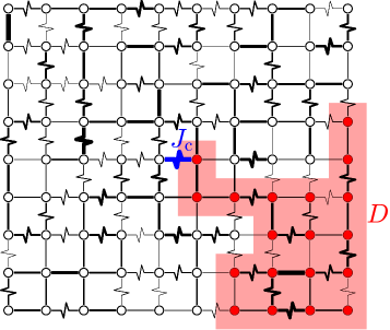
Figure 1: (Color online.) Illustration of our numerical experiments for the square lattice. The straight-line and crossed bonds represent ferromagnetic ($J_{ij}>0$) and anti-ferromagnetic ($J_{ij}<0$) bonds, respectively. The thickness of the bonds increases with $|J_{ij}|$. On the two sides of a critical value $J_{\mathrm{c}}$ of the coupling of the central bond $(i_{0},j_{0})$ (highlighted in blue), two different ground-states occur which differ by a domain $D$ of flipped spins (red region). The boundary links in $\partial D$ are the bisected orthogonal edges.

Multi-droplet excitations. We may vary couplings $J_{ij}$ on general (non-central) bonds and examine their respective ZEDs and, by doing so, study general multi-droplet excitations for arbitrary ${\mathcal{J}}$. From (2), for general couplings, $\Delta E$ vanishes at “criticality” for non-trivial domains when degeneracy appears and is linear in deviations of the coupling constants from their critical values. In the thermodynamic limit, for the continuous distribution $\mathcal{P}_{J}$, any finite number of coupling constants on disjoint bonds will approach their critical values arbitrarily closely. Thus, in that limit, the critical boundary excitations that we examine and their hybrids may be of the lowest possible energy. A related result holds for arbitrary energy excitations [35].

Numerical calculations. We studied ZEDs by computing ground-states of the EA Ising model on (free boundary condition) square, triangular, and honeycomb lattices of linear size $L=16,\ldots,128$, cubic lattices with $L=5,6,7$, the body-centered cubic system with $L=5$, and $z$-regular random graphs (RRGs) of coordination number $z=3$, $4$ and $6$ with $N=128$ nodes. For each specific lattice or graph, we used $\sim 10^{5}$ bond configurations (disorder samples) for averaging [35]. For all planar spin-glasses, we use the polynomial-time minimum-weight perfect matching method [36, 37] with Blossom V [38] to determine exact ground-states. For non-planar systems, an exact branch-and-cut approach (implemented with Gurobi [39]) executes a brute force search tree examination of all possible spin configurations. All of the code that we used for this work is publicly available .

Droplet energies and critical couplings. When the central coupling $J_{i_{0}j_{0}}$ varies from an initial strength of $J_{0}$ across $J_{\mathrm{c}}$ to a new value, the corresponding ground-state of (1) transitions from ${\cal{C}}$ to ${\cal{C}}^{\prime}$. As seen from the perspective of the original system with the initial coupling $J_{i_{0}j_{0}}=J_{0}$, the configuration ${\cal{C}^{\prime}}$ constitutes an excitation of energy $\Delta E=2|J_{0}-J_{\mathrm{c}}|$ above that of the ground-state ${\cal{C}}$. Using the latter relation for $\Delta E$, we inferred $J_{\mathrm{c}}$ by comparing the ground-states found for $J_{i_{0}j_{0}}\ll 0$ and $J_{i_{0}j_{0}}\gg 0$ respectively. In Fig. 2(a), we present excitation energies $\Delta E$ for the $d=2$ and $d=3$ lattices as well as the RRGs. The distributions are unimodal peaking close to $\Delta E=0$, with the energy changes increasing with the lattice (or graph) coordination number $z$. As the inset shows for the example of the square lattice, the distributions are almost perfectly independent of the lattice or graph size. Hence there is no scaling of the excitation energies with system size. To better understand these distributions, we examined the behavior of the critical couplings $J_{\mathrm{c}}$. As their probability density is even [35], in Fig. 2(b) we show the distribution of the modulus $|J_{\mathrm{c}}|$. These distributions are well described by a stretched exponential (or stretched Gaussian) [35]

Table 1: Parameters of the stretched exponential (3), as well as values of the scaling exponents $\kappa_{\mathrm{v}}$ of Eq. (4) for the droplet volume and $\kappa_{\mathrm{s}}$ of (5) for the droplet boundary, for the different lattices considered listed in ascending order of their coordination number.

Lattice	$a_{\mathrm{c}}$	$\beta_{\mathrm{c}}$	$\kappa_{\mathrm{v}}$	$\kappa_{\mathrm{s}}$
honeycomb	$2.76(1)$	$1.59(1)$	$0.212(1)$	$0.34(2)$
square	$1.204(9)$	$1.68(1)$	$0.214(1)$	$0.334(1)$
triangular	$0.532(9)$	$1.78(1)$	$0.21(1)$	$0.327(2)$
simple cubic	$0.61(1)$	$1.74(2)$	$0.127(1)$	$0.163(2)$
bcc	$0.212(5)$	$1.79(1)$	$0.103(1)$	$0.131(1)$

$$P(|J_{\mathrm{c}}|)=k_{\mathrm{c}}\exp(-a_{\mathrm{c}}|J_{\mathrm{c}}|^{\beta_{\mathrm{c}}}),$$ (3)

with $1<\beta_{\mathrm{c}}<2$. The lines in Fig. 2(b) show fits of this form with the parameters collected in Table 1. The typical values for $J_{\mathrm{c}}$ are mostly determined by the lattice/graph coordination number $z$; the distributions almost collapse if plotted as a function of $|J_{\mathrm{c}}|/z$, cf. the inset of Fig. 2(b). For instance, data for the ($z=6$) cubic lattice nearly collapse onto those of the ($z=6$) triangular lattice. Similarly, the $P(|J_{\mathrm{c}}|)$ distributions for RRGs of fixed coordination $z=3$, $4$, $6$ but having, otherwise, random structure match with their counterparts of the honeycomb, square, and triangular lattices respectively. Deviations are most pronounced for small $z$. This is most apparent for the one-dimensional chain ($z=2$) for which $P(|J_{\mathrm{c}}|)=\delta(|J_{\mathrm{c}}|)$ (since any sign change of the central coupling $J_{i_{0}j_{0}}$ generates a new ground-state in which all spins on one side of the central bond are flipped with degenerate ground-states at $J_{i_{0}j_{0}}=0$). Asymptotically, $P(|J_{\mathrm{c}}|)$ is independent of boundary conditions, although finite-size corrections might be strong [35]. In addition to tuning the central coupling $J_{i_{0}j_{0}}$ to its critical value $J_{\mathrm{c}}$ at which degenerate ground-states appear, we observed that the probability that the ground-state does not change when the initial central coupling is flipped ($J_{i_{0}j_{0}}\to-J_{i_{0}j_{0}}$) increases with the density of closed loops [35].

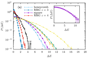
Figure 2: (Color online.) The color legends apply to both panels. (a) Probability densities for the excitation energies $\Delta E$ for the different lattices and graphs considered. The inset shows the distributions for square lattices of sizes $L=16$, $32$, $64$ and $128$ (darker shades for larger systems), illustrating that they are almost perfectly independent of system size. (b) Probability densities of the modulus of the critical coupling, $|J_{\mathrm{c}}|$, together with fits of the stretched exponential form (3) to the data. Curves for lattices/graphs of the same coordination number $z$ are nearly indistinguishable. The inset shows the distributions as a function of $|J_{\mathrm{c}}|/z$.

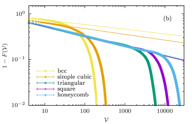
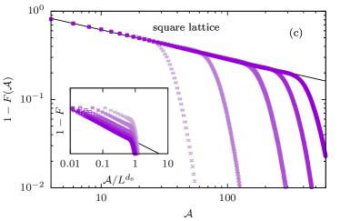
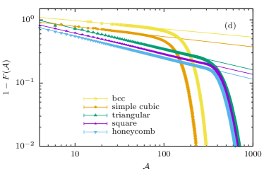
Figure 3: (Color online.) ZED volume $\mathcal{V}$ and surface area $\mathcal{A}$ distributions. (a) Distribution of ZED volumes for square lattices of sizes $L=16$, $32$, $64$, $96$ and $128$ (darker shades correspond to larger systems). The inset shows the tails with the ordinate rescaled by $L^{d_{\mathrm{v}}}$ with the volume fractal dimension $d_{\mathrm{v}}=2$. (b) Volume distributions for the different lattice types with fits of the power-law form (4). (c) Tails of the ZED surface areas for square lattices. The inset shows a rescaling of the ordinate with $L^{d_{\mathrm{s}}}$ for $d_{\mathrm{s}}=1.273$. (d) Surface area distribution for different lattices with fits (5).

Droplet volumes and boundary areas. Having established the non-scaling or $O(1)$ nature of the energies, we next study the ZED geometries. In Fig. 3(a), we show the tail distribution of the number of sites $|D|$ in these droplets (or volume) for square lattices of sizes $L=16$, $32$, $64$, $96$ and $128$. All tails follow a power-law successively extending to larger droplet volumes $\mathcal{V}$,

$$P(|D|\geq\mathcal{V})=1-F(\mathcal{V})=k_{\mathrm{v}}\mathcal{V}^{-\kappa_{\mathrm{v}}},$$ (4)

where $F$ is the cumulative distribution function. Once the ZEDs become too large, $\mathcal{V}\gtrsim\mathcal{V}_{0}(L)$, the finite size of the system becomes manifest and the probability plummets far more rapidly with the ZED size. As illustrated in Fig. 3(b), we find similar power-laws for all considered $d=2$ and $d=3$ lattices. The decay exponent $\kappa_{\mathrm{v}}$ predominantly depends only on the lattice dimension and no other geometrical details. Thus, we find the compatible $\kappa_{\mathrm{v}}\approx 0.33$ for the square, triangular, and honeycomb lattices, and $\kappa_{\mathrm{v}}\approx 1.3-1.6$ for the simple cubic, and bcc lattices, respectively. The individual fit values appear in Table 1. By comparison to their planar counterparts, the more notable differences between the simple cubic and bcc lattices may be a consequence of the smaller size of the $d=3$ lattices that we were able to examine.

The ZED surface areas $|\partial D|$ exhibit a similar power-law distribution

$$P(|\partial D|\geq\mathcal{A})=1-F(\mathcal{A})=k_{\mathrm{s}}\mathcal{A}^{-\kappa_{\mathrm{s}}}.$$ (5)

As seen in Fig. 3(c), deviations from the power-law behavior occur for $\mathcal{A}\gtrsim\mathcal{A}_{0}(L)$ with $\mathcal{A}_{0}(L)$ monotonically increasing in $L$ . As apparent from Fig. 3(d), the exponents $\kappa_{\mathrm{s}}$ are again universal, depending only on the lattice dimension, cf. the fit parameters collected in Table 1. For RRGs with sparse closed loops, $P(|\partial D|\leq\mathcal{A})$ becomes very sharp. For tree-like graphs (no closed loops), an entire branch of spins attached to the central bond flips when $J_{i_{0}j_{0}}$ changes sign. Here, the boundary separating the ground-states for positive and negative $J_{i_{0}j_{0}}$ is comprised of only one ($|\partial D|=1$) bond and $P(|\partial D|\leq\mathcal{A})$ increases sharply (a step function). Similarly, a higher exponent $\kappa_{\mathrm{s}}$ (sharper $P(|\partial D|\leq\mathcal{A}$) appears for lattices of lower spatial dimension $d$ having fewer closed loops (see Table 1). The analysis of the $d=1$ lattice is identical to the tree-like graphs leading to a step function $P(|\partial D|\leq\mathcal{A})$.

Fractal dimension. Analyzing, for the square lattice, the scaling of the ZED volume and surface areas with their linear extent, we deduce a volume fractal dimension $d_{\mathrm{v}}=1.954(8)$ and a surface fractal dimension $d_{\mathrm{s}}=1.24(2)$ [35]. To avoid large error bars, we restricted fits to $\ell\geq\ell_{\min}=40$, where $\ell$ denotes the linear ZED size [35]. When allowing for additional power-law (in $\ell$) corrections to the ZED volumes and surface areas, the leading terms (yielding the above fractal dimensions) did not change significantly. ZEDs are hence (at least very nearly) space-filling with fractal surfaces of Hausdorff dimension compatible with that of domain-walls induced by changes of the boundary conditions, $d_{\mathrm{s,DW}}=1.2732(5)$ [43]. This similarity of fractal dimensions is intuitive as the flipping of boundary couplings involved in transitioning from periodic to antiperiodic boundary conditions is akin to a sequence of ZED flips . Indeed, the injection of a domain-wall can be viewed as sequentially flipping the bonds, one after the other, along a system boundary. The ground-state changes in a similar way following any of the individual bond flips so a similarity amongst the two Hausdorff dimensions might be natural [35].

Given the cumulative power-law tail distributions of (4) and (5), it is clear that the probability densities of volumes and surface areas decay algebraically (with exponents $\kappa_{\mathrm{v}}+1$ and $\kappa_{\mathrm{s}}+1$, respectively) implying that the average volume $\langle\mathcal{V}\rangle$ and surface area $\langle\mathcal{A}\rangle$ diverge with $L$. Specifically, the power-law ($\propto\mathcal{V}^{-(\kappa_{\mathrm{v}}+1)}$) regime of the ZED volume distribution implies the lower bound $\langle\mathcal{V}\rangle>\int_{0}^{\mathcal{V}_{0}}d\mathcal{V}\,\mathcal{V}^{-\kappa_{\mathrm{v}}}/\int_{0}^{\mathcal{V}_{0}}d\mathcal{V}\,\mathcal{V}^{-(\kappa_{\mathrm{v}}+1)}\propto\mathcal{V}_{0}$. There are additional $\mathcal{V}>\mathcal{V}_{0}$ contributions not following the power-law form (4). The scaling collapse in the inset of Fig. 3(a) illustrates that $\mathcal{V}_{0}\sim L^{d_{\mathrm{v}}}$ such that the average volume diverges rapidly with $L$. Likewise, $\langle\mathcal{A}\rangle\sim L^{d_{\mathrm{s}}}$. Hence critical ZEDs are excitations of divergent length scales with fractal boundaries.

Discussion. The ground-states of the Gaussian EA Ising model are exceedingly fragile and respond with (ZED) excitations of unbounded size to perturbations of single exchange couplings. We find universal exponents governing the geometrical size of these excitations, the distribution of (“critical”) single bond coupling constants at which ground-state degeneracies occur, and energies. In the thermodynamic limit, many couplings are inevitably arbitrarily close to being critical such that an infinitesimal amount of energy suffices to create macroscopic system spanning excitations. All possible excitations (domain-wall or other) may be associated with ZEDs that appear as exchange constants are sequentially tuned to values that they assume when these excitations arise [35]. The energies of system spanning $d=2$ domain-wall excitations of length $\ell$ vanish as $\ell^{\theta}$ with $\theta=-0.2793(3)<0$ [43] thus asymptotically approaching, for large $\ell$, those of ZEDs. When keeping the couplings fixed, spin configurations associated with (generally system spanning) single bond ZEDs constitute excitations of energies that do not scale with $L$. In $d=3$ or whenever $\theta>0$, domain-wall excitation energies diverge with increasing $L$ and are thus less relevant for the physics at low temperatures.

In $d=2$ and $d=3$ lattices, the ZED volume and surface area distributions follow universal power-laws with finite lattice cutoffs. ZEDs have compact volumes with Hausdorff dimensions consistent with those of the lattice yet with fractal boundaries of a dimension consistent with that of domain-wall excitations in $d=2$.

Our setup for investigating ZEDs is complementary to that for “disorder chaos” wherein randomness is introduced globally by perturbing all couplings in the system [45, 46, 47, 48, 49, 50]. This leads to an energy contribution proportional to $\ell^{d_{\mathrm{s}}/2}$. According to droplet theory, the relevant energy scale is $\Delta E\propto\ell^{\theta}$, suggesting disorder chaos whenever $d_{\mathrm{s}}/2>\theta$. By their very nature, ZED perturbations (whose existence is guaranteed in the thermodynamic limit) are always relevant low-energy excitations.

Since vanishing energy excitations are composites of ZEDs, our findings carry important consequences. Notably, the features of these elementary spin-glass excitations are at odds with prevailing theories. The energies of macroscopic ZEDs are inconsistent with the droplet and chaotic-pairs pictures. Although finite-size corrections can be strong for spin-glasses, the power-law exponents in Table 1 clearly indicate divergent droplet sizes in $d=2$ and $d=3$. In the regime accessible to our simulations, ZEDs clearly do not feature space-filling boundaries stipulated by RSB. The search for theories of the spin-glass phase that are consistent with these observations hence seems a rewarding target for further research.

Acknowledgements. We wish to thank Gilles Tarjus for a discussion. ZN is grateful to the visiting Leverhulme-Peierls Professorship at Oxford University. Part of this work was performed at the Aspen Center for Physics, which is supported by National Science Foundation grant PHY-2210452.

Supplemental Material

I Numerical Settings

In Table 2 we provide the size and number of samples of each kind of lattice investigated.

Table 2: The system linear size $L$ (or number of nodes for RRGs) for each lattice and the corresponding number of samples are listed here.

Lattice	$L$	$N_{\text{sample}}$
honeycomb	$[16,32,64,96,128]$	$[10^{5},10^{5},10^{5},85395,10^{5}]$
square	$[16,32,64,96,128]$	$[10^{5},10^{5},10^{5},10^{5},10^{5}]$
triangular	$[16,32,64,96,128]$	$[10^{5},10^{5},10^{5},10^{5},101318]$
simple cubic	$[5,6,7]$	$[40792,32297,32205]$
bcc	$5$	$55744$
RRG $z=4$	$128$	$10^{5}$
RRG $z=6$	$128$	$10432$
RRG $z=10$	$128$	$2817$

All of our numerically provided distributions (such as those of the critical couplings and ZED volumes and areas) and their associated averages (e.g., average ZED volumes and areas and their fractal dimension scaling) were computed over the sample realizations of the spin-glass Hamiltonian of Eq. (1). As discussed in the main text, in these sample realizations, couplings $J_{ij}$ were drawn with probability density ${\mathcal{P}}_{J}(J_{ij})=(1/\sqrt{2\pi})\exp(-J_{ij}^{2}/2)$.

II Proofs of finite energy changes and other properties

We now briefly prove properties (i)- (iii) of the main text. A violation of (i) implies that flipping all spins in $D$ (that does have the central bond as part of its boundary) creates a degenerate ground state at the critical coupling $J_{i_{0}j_{0}}=J_{\mathrm{c}}$. If $\partial D$ does not involve the central bond, this indicates that the original configuration with the unaltered $J_{i_{0}j_{0}}=J_{0}$ was degenerate with another ground state. However, apart from a set of vanishing measure in the coupling constants, the Gaussian EA Ising system is non-degenerate [13]. Statement (ii) may be similarly proven by contradiction. Indeed, if additional transitions (apart from the one at $J_{i_{0}j_{0}}=J_{\mathrm{c}}$) between other degenerate ground states appeared in either of the two regimes in which both spins belonging to the central bond were either of the same or opposite relative orientation then these would only involve a change of other spins that do not belong to the central bond (thus violating (i)). To establish (iii), we recognize that although the ground state exhibits a change from a global spin configuration ${\cal{C}}^{-}$ at $J_{i_{0}j_{0}}<J_{\mathrm{c}}$ to a configuration ${\cal{C}}^{+}$ at $J_{i_{0}j_{0}}>J_{\mathrm{c}}$ (possibly involving a divergent number of spins having different assignments in the two respective ground states), the energy of any of the $2^{N}$ Ising spin configurations is, as a function of the coupling constants $\{J_{ij}\}$, linear. Thus, the minimum energy amongst these states is a continuous function of the coupling constants. Therefore, regardless of whether ${\cal{C}}^{-}$ and ${\cal{C}}^{+}$ differ by an extensive number of flipped spins (numerically, we find that the number of such flipped spins is indeed extensive), the ground-state energy is a trivial linear function of $J_{i_{0}j_{0}}$ as seen in (2).

(A) If the initial and final values of the central coupling constant are both larger than $J_{\mathrm{c}}$ or if both are smaller than $J_{\mathrm{c}}$ then varying the central coupling constant between these initial and final values will not change the ground-state and thus the energy, as evaluated with the original value $J_{0}$ of the central coupling constant, will identically correspond to a vanishing energy change: $\Delta E=0$.

(B) We next briefly consider what transpires if the initial and final values of the central coupling constant lie on different sides of $J_{\mathrm{c}}$ (one being smaller than $J_{\mathrm{c}}$ and the other being larger than $J_{\mathrm{c}}$). The energy change can be readily computed with the aid of (2) where now $D$ is the domain (ZED) of spins that differ in ${\cal{C}}^{-}$ and ${\cal{C}}^{+}$. By definition, precisely at criticality, the states ${\cal{C}}^{-}$ are ${\cal{C}}^{+}$ are degenerate and (2) vanishes. As we vary the central coupling from $J_{c}$ to the value $J_{0}$ that it assumes in the initial Hamiltonian, only the term involving the central bond will change in the sum of (2). That is, $\Delta E$ will increase from its vanishing value at criticality as $\Delta E=2|J_{0}-J_{c}|$.

Thus, if distribution of $J_{c}$ values ($P(J_{c})$) tends to well defined (system size independent) form in the thermodynamic limit (which numerically it indeed is (see the inset of Fig. 2 (a)) then so is that of the associated energy changes ($P(\Delta E)$). As described in the main text, (B) was used to determine $J_{\mathrm{c}}$. While the statistical properties of $J_{\mathrm{c}}$ may depend on the system size for small systems, the latter energy change will always be of order unity (i.e., not increase with the system size since the coupling constants do not diverge with the lattice size). Similarly, as we further detail in this Supplementary Material, for the “Repulsive Boundary Conditions” there is a weak correlation between $J_{\mathrm{c}}$ and the associated ZED boundary area $|\partial D|$. We numerically find that the distribution $P(J_{\mathrm{c}})$ of critical coupling constants approaches a well-defined limit for large $L$. Given such a $P(J_{\mathrm{c}})$, both energy changes (A) (which does not depend on $J_{\mathrm{c}}$) and (B) will veer towards system size independent values for large $L$. That is, the distribution of the energy changes will tend to a unique form in the thermodynamic limit.

III Flipping the Sign of Central Bond and Probability of Changing the Ground State

We now ask what will transpire if we flip the sign of the central bond $J_{i_{0}j_{0}}$ in the initial state (sampled from the Gaussian distribution of ${\cal{P}}_{J}$) rather than tune its value to the critical coupling value $J_{\mathrm{c}}$ at which the ground-state transition appears. Let us explicitly write the associated CDF as $F(J_{\mathrm{c}})\equiv\int_{0}^{|J_{\mathrm{c}}|}P(|J^{\prime}_{\mathrm{c}}|)dJ^{\prime}_{\mathrm{c}}$. By construction, $F(J_{\mathrm{c}})$ is the probability that the critical coupling $J^{\prime}_{\mathrm{c}}$ lies within the interval $[-|J_{\mathrm{c}}|,|J_{\mathrm{c}}|]$. We may express the probability of changing the ground-state (G.S.) as

$$P ({\text{G.S. Change}})=\int^{\infty}_{0}\mathcal{P}_{J}(J_{i_{0}j_{0}})~{}F(J_{i_{0}j_{0}})~{}dJ_{i_{0}j_{0}}$$ (6)

$$=\int^{\infty}_{0}dJ_{i_{0}j_{0}}\frac{1}{\sqrt{2\pi}}e^{-\frac{J_{i_{0}j_{0}}^{2}}{2}}\int_{0}^{|J_{i_{0}j_{0}}|}dJ_{\mathrm{c}}~{}~{}2P(|J_{\mathrm{c}}|).$$

Eq. (6) relates the $J_{\mathrm{c}}$ distributions to the probabilities of changing the ground-states when we flip the central bond. In Table 3, we list the such probabilities for different types of lattices and different system sizes. Note the system sizes are different from what we have in Table 2; this is another computation in which we forcefully flip the bond, rather than tune it to $J_{\mathrm{c}}$.

	8	28	48
$d=2$ honeycomb	0.2506	0.2525	0.2534
$d=2$ square	0.3795	0.3744	0.3781
$d=2$ triangular	0.5110	0.5133	0.5104
	3	5	7
$d=3$ simple cubic	0.4748	0.4887	0.4904
	2	3	4
$d=3$ bcc	0.6218	0.6604	0.6685

Table 3: The probability of changing the ground state $P({\text{G.S. Change}})$ following a flip of the sign of the initial random value of the central bond ($J_{i_{0}j_{0}}\to-J_{i_{0}j_{0}})$.

IV The distribution $P(|J_{\mathrm{c}}|)$ of critical couplings for decoupled loops

In what follows, we motivate a function that is very similar (when $|J_{c}|\lesssim 1$) to that of Eq. (3) for the particular (exactly solvable) case of decoupled loops of uniform fixed length. Towards this end, we define the conditional probability $Q(J)\equiv P(\sigma_{i}\sigma_{j}=+1|J_{ij}=J)$. Namely, $Q(J)$ is the probability that $\sigma_{i}\sigma_{j}$ assumes the value of $+1$ given that the link strength between the two spins is equal to $J$. Note that $Q(J)$ is, in fact, the cumulative distribution function of $J_{\mathrm{c}}$. That is, $Q(J)$ allows us to infer the probability that $J_{\mathrm{c}}<J$. That is,

$$P(J_{\mathrm{c}})=Q^{\prime}(J_{\mathrm{c}}).$$ (7)

At the critical coupling strength $J_{\mathrm{c}}$, the product $\sigma_{i}\sigma_{j}$ changes sign.

We next investigate individual closed loops formed of $M$ individual bonds (e.g., $M=3$ for a single triangular plaquette, $M=4$ for a minimal square plaquette, etc.). Without loss of generality, for a particle bond $(ij)$, we consider $J_{ij}=J>0$. Whether closed loops are “unfrustrated” (i.e., all bonds in Eq. (1) can be simultaneously minimized) or “frustated” (when they cannot) depends on whether they respectively have an even or odd number of negatively valued couplings $J_{ab}$. For an unfrustrated closed loop, every single bond can be satisfied and thus for the specific link at hand, $\sigma_{i}\sigma_{j}=+1$. Within the ground-state of a frustrated closed loop, the link of the smallest absolute value $|J_{\min}|\equiv|J_{a^{*}b^{*}}|\equiv\min_{ab\in{\sf{loop}}}\{|J_{ab}|\}$ will be unsatisfied (that is for that link the product $J_{a^{*}b^{*}}\sigma_{a^{*}}\sigma_{b^{*}}<0$). Therefore, $\sigma_{i}\sigma_{j}=+1$ if and only if $|J_{ij}|$ is not the smallest bond among the $M$ bonds forming the closed loop, $|J|>|J_{\min}|$. Given that each of the $M$ links are drawn from the normal distribution ${\mathcal{P}}_{J}(J_{ab})=(1/\sqrt{2\pi})\exp(-J_{ab}^{2}/2)$, the probability that $J_{ij}$ is not the smallest coupling in absolute value amongst the $M$ coupling in the loop is, trivially, $1-(1-\frac{1}{\sqrt{2\pi}}\int_{-J}^{J}dJ^{\prime}e^{-(J^{\prime})^{2}/2})^{M-1}$. Thus, for a single loop of length $M$,

$$Q(J)=1-(\mathrm{erfc}(J))^{M-1},$$ (8)

with $\mathrm{erfc}(J)$ the complementary error function. Eq. (7) then enables us to determine the probability distribution $P(J_{c})$ of critical couplings. Numerically, when constrained to the interval $|J_{c}|\leq 0.8$, except for exceedingly small arguments, the derivative of Eq. (8) (i.e., $P(J_{c})$ for decoupled loops) can be made to match exceptionally well the empirical stretched exponential (or stretched Gaussian) distribution (Eq. (3) of the main text), see Fig. 4 (a). The difference between our exact result for decoupled loops with the fitted (for measurable probability densities) empirical general lattice and graph form of Eq. (3) becomes far more acute when the $|J_{c}|$ interval is an order of magnitude larger. Indeed, as seen in panel (b) of Fig. 4, the critical probabilities predicted by Eq. (3) where the latter are fitted to Eqs. (7, 8) when $P(J_{c})$ is finite and measurable) become exceedingly small for very large $|J_{c}|$.

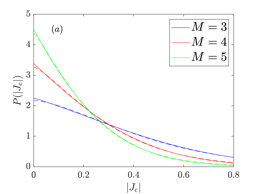
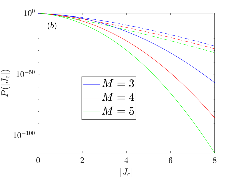
Figure 4: (Color online.) The exact critical coupling distribution of Eqs. (7, 8) (solid lines) for decoupled closed loops of length $M$ fitted by Eq. (3) (dashed lines). (a) When $|J_{c}|<0.8$ and the probability density $P(|J_{c}|)$ is of order unity, one sees an exceptional agreement between the exact result of Eqs. (7,8) for decoupled loops (dashed lines) and the more general numerical fit of Eq. (3) (solid lines). This agreement is evident for all but the smallest values of $|J_{c}|$. (b) When examined over the far broader range $|J_{c}|<8$, there are very notable differences (on a logarithmic scale) between the exact result for decoupled loops and the numerical fit (of Eq. (3)) to that result. Note that the deviation shown is on a logarithmic scale. In terms of absolute size, both Eqs. (7, 8) and well as the continuation of the empirical form of Eq. (3) (when the latter is fitted in (a) to the exact result (Eqs. (7, 8)) for decoupled loops for $|J_{c}|<0.8$) to larger $|J_{c}|$ values are, literally, exponentially close to zero and should be completely unobservable. Empirically, however, the numerically measurable $P(J_{c})$ is not nearly as small (see Fig. 2(b)). This discrepancy illustrates that the exact result for decoupled closed loops (Eqs. (7, 8) misses essential features of the full lattice (and graph) systems that are correctly captured by Eq. (3).

This disparity is not surprising. We must indeed underscore that the above derivation of Eq. (8) applies for a single closed loop and thus, by extension, only to decoupled loops of uniform length $M$. Clearly, the full problem on the lattice/graph in the thermodynamic limit is not that of the limiting case of decoupled loops of fixed length for which Eq. (8) is exact. Thus, the scaling collapse of the $P(J_{c})$ curves in the inset of Fig. 2(b) highlighting the lattice/graph coordination number and the success of Eq. (3) in describing RRGs for which only non-uniform sparse loops may appear does not, at all, follow from the above exact result for decoupled loops. It is for all of these reasons that we employed, in the main text, the more generic stretched exponential (or stretched Gaussian) fit of Eq. (3) that numerically works well over the entire very broad numerically tested spectrum of $|J_{c}|$ values (see Fig. 2(b)) and captures the coordination number dependence of $P(J_{c})$ (Fig. 2(b) and its inset).

V The Fractal Dimension of Critical Droplets

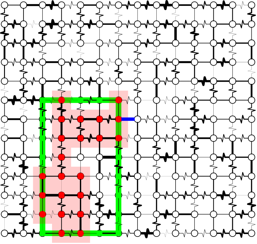
(a) Minimal Rectangle Cover (green rectangle). In this approach for determining the fractal dimension of the ZED (red) generated by the flip of the central bond (blue), the longer edge of this rectangle is defined as the linear size.

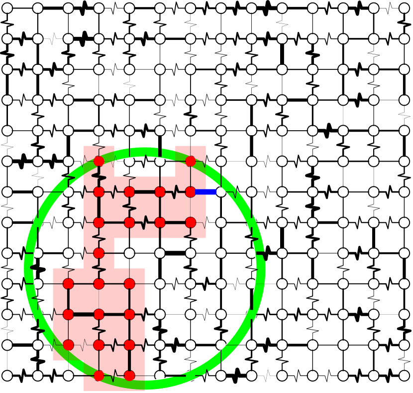
(b) Minimal Circle Cover (green circle). In a second approach for determining the fractal dimension of the ZED (red), the radius of this circle is defined as the linear ZED size.

Figure 5: (Color online.) Two different ways for defining the linear size of the ZED. Both ways led to numerically similar results for the deduced fractal dimension.

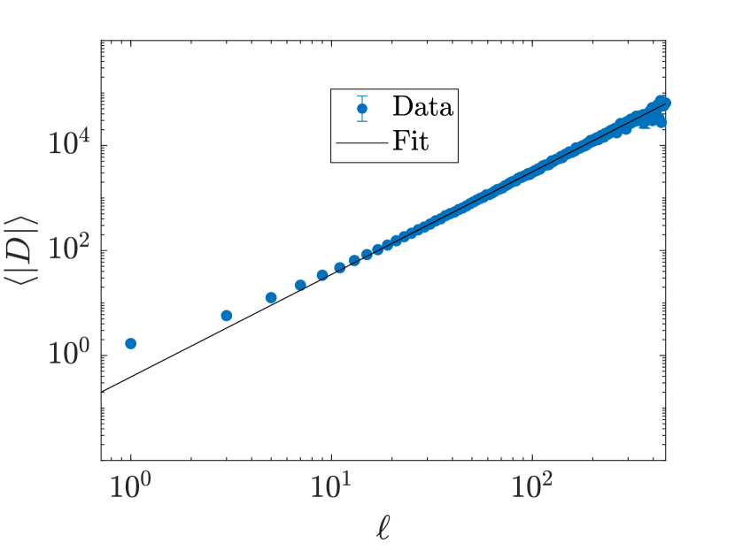
(a) Average ZED volume size as a function of its linear size.

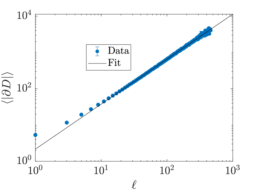
(b) Average ZED boundary area as a function of the ZED linear dimension.

Figure 6: (Color online.) Fractal dimensions fits. We binned data for different linear sizes (see definitions in Fig. 5) and computed the associated average volume/boundary areas. A power-law fit (linear fit on the shown log-log scale) for the dependence of the volume/boundary area on the linear size $L$ (allowing for a determination of the respective volume and area fractal dimensions) was then applied. The smallest possible $\ell$ is that of one bond. Examining the slope of best fit to the data in an interval $[\ell_{\min},L]$ in the above log-log plots led to the fractal dimensions displayed in Fig. 7.

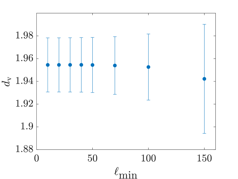
(a) The dependence of the numerically determined volume fractal dimension on the linear sizes of the ZEDs that are examined.

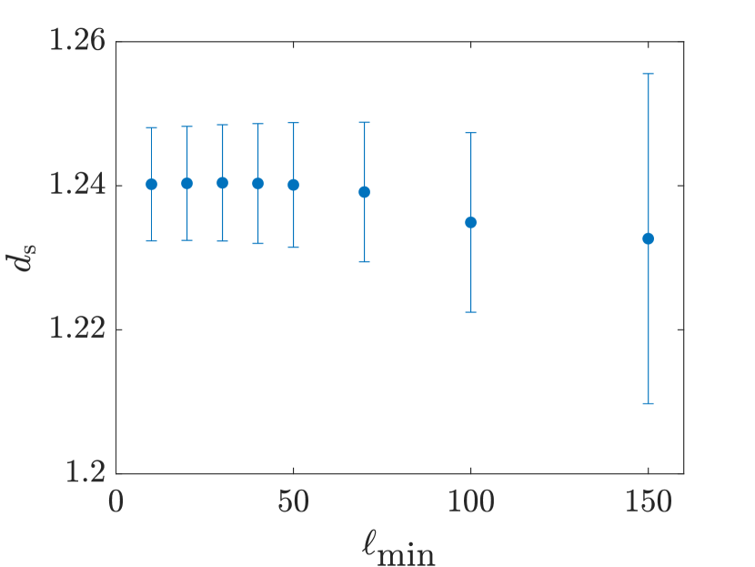
(b) The dependence of the numerically determined boundary area fractal dimension on the ZED linear sizes employed.

Figure 7: (Color online.) The numerically obtained fractal dimensions (see also Fig. 6) for an illustration of the power law fits enabling the determination of the fractal dimensions) when fitted for ZEDs of linear size $[\ell_{\min},L]$. The larger error bars that appear as $\ell_{\min}$ grows are a consequence of concomitantly having smaller data sets containing ZEDs of linear size $\ell_{\min}\leq\ell\leq L$ as $\ell_{\min}$ is increased.

The fractal dimension of the critical droplets describes how the extension of the critical droplets, e.g., the boundary length or the volume, could depend on its linear size.

For a single droplet, there might be multiple ways to define its linear size $l$. For the shown square systems, we comprehensively analyzed two different settings, see Fig. 5:

• Minimal Rectangular Cover. A minimal rectangle(green) that covers the droplet is found. Then, we take the longer edge as the linear size of the droplet.

• Minimal Circle Cover. A minimal circle(green) that covers the droplet is found. In other words, in this case the linear size is defined as the longest Euclidean distance between all the possible pairs of spins in the droplet.

For both the rectangular and circle covering settings, we found similar fractal dimensions, see text. In the current work, we adopted the second setting to define the linear size.

We consider the droplets of a $512\times 512$ square lattice with $84,524$ samples. In this analysis, we adopted the Kasteleyn cities algorithm [37] that enabled us to examine large systems. The fractal dimensions were then extracted from the dependence of the average ZED volume and surface area on its linear extent (see Fig. 6, 7). In computing the fractal dimension of the ZEDs, one should be aware of numerical details may influence the final result:

• The binning size $\ell_{\text{bin}}$. We have to bin the linear size so we can compute the corresponding average droplet size. We set it to be $\ell_{\text{bin}}=2.0$.

• The fitting range $\ell\geq\ell_{\min}$. In [43], to compute the fractal dimension of $d=2$ domain-walls, the authors used the domain-walls with $L\geq 40$, which could reduce the finite-size effect. Here, we adopted the similar setting. The linear size is restricted to $\ell\geq\ell_{\min}=40$. To see how different $\ell_{\min}$ may influence the numerically extracted fractal dimension, in Fig. 7, we show the so-determined fractal dimensions as a function of $\ell_{\min}$.

Employing such a numerical procedure, we show the deduced fractal dimensions in Fig. 7. In the main text and below, we provide the results obtained when fitting all ZEDs having a linear dimension $40=\ell_{\min}\leq\ell\leq L=256$. For a circular covering, the volume (i.e., number of sites in the square lattice ZEDs) and area (i.e., perimeter or number of bonds for ZED boundary on the square lattice) fractal dimensions are, respectively, $1.954(8)$ and $1.24(2)$. Form the rectangular coverings, these values are $1.96(1)$ and $1.25(1)$. (We recall, for comparison, that the domain-wall boundary area fractal dimension is $1.2732(5)$ [43].) In the main text, we quote the values obtained for a circular covering. We further tested what occurs when allowing for sub-leading corrections to the ZED volume or area power law fits on their linear size. We find that the fractal dimensions associated with such sub-leading terms fluctuate greatly leading to $d_{\mathrm{v}}=-0.7$ and $d_{\mathrm{s}}=-0.9$ with unacceptably large error bars ($22.3$ and $4.9$, respectively). These results suggest that sub-leading corrections are spurious and that the size of the ZED volume and surface area is indeed captured by the respective volume and area fractal dimensions.

VI Repulsive and half periodic boundary conditions

We now discuss the role of boundary conditions in some detail. In the results that we reported on in the main text, we used open boundary conditions. For comparison with earlier work, however, [31], we also employed what we call ‘repulsive boundary conditions’. Herein, the boundary spins are kept fixed so that, by construction, the droplets cannot reach (and are effectively repelled by) the boundary. Our analysis reveals that the divergent (in size) ZEDs and the exponents that we find might be more readily missed, due to finite size effects, by the use of these boundary conditions. Perusing ours and earlier numerical results with these boundary conditions [31], one finds that if only the largest system sizes are employed with droplets lying well within in the system bulk, then these will agree with those using open boundary conditions. The value of the critical coupling $J_{\mathrm{c}}$ exhibits a weak correlation with the droplet size. To elucidate this weak effect, we investigated three different settings: (a) free, (b) half-periodic, and (c) repulsive boundary conditions on various quantities. In Fig. 8, we plot, for square lattices of varying size, the difference between the original system and that arrived at by tuning the central bond $J_{i_{0}j_{0}}$ to the critical value $J_{\mathrm{c}}$. The energy difference between the initial and final ground states is computed with the same initial set of coupling constants (that with $J_{0}$). As seen in Fig. 8, for the largest system, there is no effect of the boundary conditions and all curves tend to a constant. However, if one tries to fit the data for the repulsive boundary conditions over all (including small) system sizes then it may seem that there is a non-trivial drop. For the open boundary condition square, honeycomb, triangular, cubic, and bcc lattices, the average single bond excitation energies are, respectively, 1.9463, 1.7452, 2.3375, 2.2531, and 3.2386 (with standard deviations of 0.0047, 0.0042, 0.0056, 0.0096, and 0.0106). As we explained earlier, when the value of $J_{i_{0}j_{0}}$ is varied, the associated change of the ground-state energy (as evaluated with the original coupling) is either (A) $\Delta E=0$ or (B) $\Delta E=2|J_{0}-J_{\mathrm{c}}|$.

Thus, the only way in which a dependence on system size can arise is if $J_{\mathrm{c}}$ depends on the system size. In Table 4, we provide, for different lattices of varying size, the Spearman correlation coefficients between the ZED boundary size $|\partial D|$ and the excitation energy $\Delta E$. As seen therein, the correlation between the two (and thus also between $J_{\mathrm{c}}$ and the droplet size) is weak and does not naturally suggest a power-law nor other types of scaling.

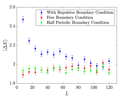
Figure 8: (Color online.) The average single bond average excitation energy $\langle\Delta E\rangle$ on $L\times L$ square lattices for (a) free boundary conditions, (b) half-periodic boundary condition and, (c) the repulsive boundary conditions (see text). For both the free boundary condition and half-periodic boundary condition, the average energy does not change systematically with the system size. For the repulsive boundary conditions, there is a nontrivial dependence of the energy on system size for small lattices before the energy difference appears to saturate (within numerical accuracy) to the very same value ($\langle\Delta E\rangle\simeq 2$) obtained with open and half-periodic boundary conditions. Note that this particular approximate limiting average value for the square lattice assumes other values for other lattices or graphs (see Fig. 2 (a) for the full distributions).

	$L$	$N_{\text{sample}}$	Correlation
honeycomb	16	$10^{5}$	-0.0050
honeycomb	96	$85395$	0.0027
square	16	$10^{5}$	-0.0010
square	96	$10^{5}$	-0.0019
square (HPBC)	16	$10^{5}$	0.0003
square (HPBC)	96	$10^{5}$	-0.003
square (RBC)	8	$10^{5}$	0.0363
square (RBC)	16	$10^{5}$	0.0263
square (RBC)	96	$10^{5}$	0.0075
triangular	16	$10^{5}$	-0.0064
triangular	96	$10^{5}$	-0.0019
simple cubic	7	$32205$	-0.013
bcc	5	$55744$	-0.018

Table 4: The Spearman correlation coefficients between the ZED boundary area $|\partial D|$ and associated critical value of the coupling $J_{\mathrm{c}}$ at which a transition between ground states appears. We list the correlations for different types of lattices. Included are also two additional boundary conditions for the square lattice: the HPBC (Half-Periodic Boundary Condition) and the RBC (Repulsive boundary condition, see text). Note the correlation coefficient is significantly larger with RBC on small $d=2$ systems.

VII Gauge symmetry and its implications

In what follows, we illustrate two simple corollaries that stem from the well-known gauge symmetry that Ising spin-glass systems possess. In particular, we will demonstrate that any spin configuration (and thus any excitation of arbitrary energy) can be generated by applying a sequence of (generally non-critical and overlapping) ZEDs.

VII.1 The even nature of the probability distribution of coupling constants

The probability distribution of the critical coupling strengths at which a ground-state transition occurs must be even. The proof of this assertion is immediate. With $i$ and $j$ denoting arbitrary nearest-neighbor sites and $t_{i}=\pm 1$, the gauge transformation

$$J_{ij}\to J^{\prime}_{ij}=J_{ij}t_{i}t_{j},~{}~{}\sigma_{i}\to\sigma^{\prime}_{i}=\sigma_{i}t_{i}$$ (9)

leaves the general spin-glass Hamiltonian of Eq. (1) invariant.

We may set $t_{i_{0}}=-1$ (with the site “$i_{0}$” marking one of the two endpoints of the central bond) leaving $t_{r\neq i_{0}}=+1$ at all other sites $r$. One can partition the space $\mathcal{J}$ of the coupling constants over the entire lattice into two: $\mathcal{J}_{>}$ and $\mathcal{J}_{<}$, depending on whether the central bond is positive or negative. We may then establish a one-to-one mapping between these two spaces, as obviously the gauge transformation of Eq. (9) is invertible. Additionally, an instance in $\mathcal{J}_{<}$, along with its ‘gauge mirror’ in $\mathcal{J}_{>}$, must have the opposite signs of $J_{\mathrm{c}}$, according to the nature of the gauge transformation. Since $\mathcal{J}=\mathcal{J_{<}}+\mathcal{J_{>}}$, the distribution of critical couplings is even $P(J_{\mathrm{c}})=P(-J_{\mathrm{c}})$. In the main text, we employed the shorthand $P(|J_{\mathrm{c}}|)\equiv P(J_{\mathrm{c}})+P(-J_{\mathrm{c}})=2P(J_{\mathrm{c}})$.

VII.2 Excitations of arbitrary energy as composites of ZEDs

The gauge symmetry of Eq. (9) implies that any Ising spin configuration ${\cal{C^{\prime}}}$ (which differs from the ground state ${\cal{C}}_{0}$ of the Hamiltonian $H$ of Eq. (1) by, say, “$s$” spin flips) can be cast as a ground state of spin-glass Hamiltonians $H^{\prime}$ for some set of coupling constants. This fact is highly significant, as it allows us to construct any spin excitation of $H$ (of either finite or vanishing energy) as a geometric composite of ZEDs appearing in a sequence of Hamiltonians,

$$H\to H^{(1)}\to H^{(2)}\to\cdots\to H^{(f-1)}\to H^{\prime}.$$ (10)

As we will explain, here, “$f$” denotes the total number of bonds that are flipped in sign in $H^{\prime}$ relative to those in $H$. (For domain-wall excitations, this number of flipped bonds is the domain-wall surface area discussed in the main text.)

To illustrate the claim embodied in (10), we may, e.g., start with the ground state ${\cal{C}}$ of Eq. (1). We then employ the gauge transformation of Eq. (9) for a single site. Taking an arbitrary site “$1$” and setting its respective gauge variable to $t_{1}=(-1)$ (with $t_{r}=1$ at all other lattice sites $r\neq\mbox{``}1\mbox{''}$) transforms the initial Hamiltonian $H\to H^{(1)}$. By comparison to $H$, the couplings $J_{1p}$ (with $p$ denoting all nearest neighbor sites of “$1$”) now change sign, $J_{1p}\to-J_{1p}$ in $H^{(1)}$. The ground state configuration of this new Hamiltonian differs from ${\cal{C}}$ by this single flipped spin (at site number “$1$”). We may then iteratively proceed in such a manner to flip another Ising spin at an arbitrary site number “$2$” and then flip another spin, etc., so as to ultimately flip any set of spins in ${\cal{C}}$. Following any such gauge transformation at the $s^{\prime}$-th step ($s^{\prime}\leq s$) in which in (9) only one single site field $t_{s^{\prime}}$ is set equal to $(-1)$ with all others being one, the $z$ links (with $z$ denoting the lattice/graph coordination number) that are attached to site $s^{\prime}$ flip their sign with all other links remaining untouched. The sign change of the former $z$ individual links may be further carried out sequentially in any order. Some of these links may be inverted multiple times as this gauge transformation is carried out site by site. Any even number of flips of a given link yields no change. In the final analysis, there is some number ($f$) of bonds that are flipped an odd number of times as the system evolves from ${\cal{C}}\to{\cal{C}^{\prime}}$; the full set of these flips realizes the gauge transformation between the two global spin configurations of ${\cal{C}}\to{\cal{C}^{\prime}}$ (Eq. (10)). Any individual flip of sign of a single link (say the $n-$th in (10) (with $n\leq(f-1)$)) generates a transformation $H^{(n)}\to H^{(n+1)}$. This single bond transformation is precisely of the form that we investigated in the current work. As the Hamiltonians evolve according to (10) (yielding the full multi-spin and link gauge transformation of (9)), the respective ground-states of change as

$${\cal{C}}\to{\cal{C}}_{1}\to{\cal{C}}_{2}\cdots\to{\cal{C}}_{f-1}\to{\cal{C^{\prime}}}.$$ (11)

We next recall our previously established property (ii). This property implied that whenever ground-state spins change when an exchange-constant $J_{ij}$ on a given bond is varied to a new value $J^{\prime}_{ij}$, these spins must belong to the ZED of the bond $(ij)$. Combining this with the fact that any spin configuration ${\cal{C^{\prime}}}$ can be cast as the ground state of some spin-glass Hamiltonian $H^{\prime}$, it follows as we will describe, a “composition” of the ZEDs appearing when individual exchange-constants $J_{ij}$ are sequentially changed will yield ${\cal{C^{\prime}}}$. That is, after the completion of this process described by (10) for all altered links $J_{ij}$, the set of spins that have been overturned a total odd number of times in the chain of Eq. (11) will form the spin excitation ${\cal{C}}^{\prime}$ of the original system $H$. We now discuss any individual part ${\cal{C}}^{(n)}\to{\cal{C}}^{(n+1)}$ of the transformation chain of Eq. (11) that is associated with the change of the $n$-th link. Here, we note that similar to our earlier discussion of property (iii), the ground-state spin configuration ${\cal{C}}^{(n+1)}$ of $H^{(n+1)}$ is either
(A) Equal to the ground-state ${\cal{C}}^{(n)}$ of $H^{(n)}$ (when the single exchange-coupling that is varied is not made to cross its critical value) or
(B) Forms a new ground state configuration which differs from ${\cal{C}}^{(n)}$ by the ZED of link $n$ (with the latter ZED delineated as it appears for the system defined by $H^{(n)}$). This arises when a critical coupling crossing does occur as the single bond flips sign.
If overlaps exist between the sets of overturned spins (i.e., the ZEDs) between any of the $f$ individual steps of the transformation of Eq. (11) then no general statements may be made regarding the energies of general excitations ${\cal{C}^{\prime}}$ (as evaluated with $H$) and their typical geometries for a given energy. However, it is worth noting that, statistically, independent of any of the Hamiltonians of (10), following each individual bond change, the geometrical characteristics of the flipped spins following each step adhere to the universal scaling relations and fractal dimensions for the volumes and surface areas that we reported on in this work. As noted in the main text, for the systems that we examined, our found fractal dimensions for single bond change ZEDs are very close to and statistically consistent with the fractal dimension of domain-walls that were generated by flipping a divergent number ($f={\cal{O}}(L)$) of links at the system boundary. In the thermodynamic limit, such asymptotically large domain-walls are composites of $f\to\infty$ (generally overlapping) individual ZEDs following the recipe of (11). We must underscore that in determining the ZED fractal dimension, we investigated (inasmuch as possible numerically) the volume and surface area scaling of the asymptotically largest ZEDs (including any such ZEDs that might be present during individual steps in sequences such as that of (11), a sequence whose length diverges for asymptotically large domain-walls).

Statistically, if the $f$ flipped bonds are far separated from one another with weak correlations amongst their respective individual ZEDs then each of the individual single bond excitation energies may be added. The latter follow the earlier discussed distribution $P(\Delta E^{\prime})$ (see Fig. 2 (a) with, for the square lattice, the average energy change $\langle\Delta E\rangle$ per bond of Fig. 8). For, e.g., such $f$ far separated bonds on a square lattice, the total mean excitation energy relative to the ground state of $H$ will be given by $f$ times the average square lattice excitation energy $\langle\Delta E\rangle$ of Fig. 8 for a single bond (i.e., by $\sim 2f$ for the square lattice).

References

- [1] M. Mezard, G. Parisi, and M. A. Virasoro, Spin glass theory and beyond. Singapore: World Scientific, 1987.
- [2] D. L. Stein and C. M. Newman, Spin Glasses and Complexity. Princeton University Press, 2013.
- [3] F. Menczer, S. Fortunato, and C. A. Davis, A First Course in Network Science. Cambridge University Press, 2020.
- [4] M. Newman, Networks: An Introduction (second Edition). Oxford University Press, 2018.
- [5] J. D. Bryngelson and P. G. Wolynes, “Spin glasses and the statistical mechanics of protein folding,” Proceedings of the National Academy of Sciences (USA), vol. 84, p. 7425, 1987.
- [6] J. A. Mydosh, Spin Glasses: An Experimental Introduction. Taylor and Francis, London, Washington D.C., 1993.
- [7] K. Binder and A. P. Young, “Spin glasses: Experimental facts, theoretical concepts, and open questions,” Reviews of Modern Physics, vol. 58, p. 801, 1986.
- [8] D. Sherrington and S. Kirkpatrick, “Solvable model of a spin-glass,” Physical Review Letters, vol. 35, p. 1792, 1975.
- [9] B. Derrida, “Random-energy model: Limit of a family of disordered systems,” Physical Review Letters, vol. 45, p. 79, 1980.
- [10] B. Derrida, “Random-energy model: An exactly solvable model of disordered systems,” Physical Review B, vol. 24, p. 2613, 1981.
- [11] D. J. Gross and M. Mezard, “The simplest spin-glass,” Nuclear Physics B, vol. 240, p. 431, 1984.
- [12] S. Edwards and P. W. Anderson, “Theory of spin glasses,” J. Phys. F, vol. 5, p. 965, 1975.
- [13] M.-S. Vaezi, G. Ortiz, M. Weigel, and Z. Nussinov, “The binomial spin glass,” Physical Review Letters, vol. 121, p. 080601, 2018.
- [14] A delicate interplay exists between the latter two (continuum coupling and thermodynamic system size) limits. These two limits do not commute with one another [13].
- [15] Degeneracies arise for special values of the coupling constants (a set of measure zero).
- [16] H. G. Katzgraber, M. Körner, and A. P. Young, “Universality in three-dimensional Ising spin glasses: A Monte Carlo study,” Phys. Rev. B, vol. 73, no. 22, p. 224432, 2006.
- [17] M. Hasenbusch, A. Pelissetto, and E. Vicari, “The critical behavior of 3D Ising glass models: universality and scaling corrections,” J. Stat. Mech.: Theory and Exp., vol. 2008, p. L02001, 2008.
- [18] S. Boettcher, “Stiffness of the Edwards-Anderson model in all dimensions,” Phys. Rev. Lett., vol. 95, p. 197205, 2006.
- [19] G. Parisi, “Infinite Number of Order Parameters for Spin-Glasses,” Physical Review Letters, vol. 43, pp. 1754–1756, Dec. 1979. Publisher: American Physical Society.
- [20] W. L. McMillan, “Scaling theory of Ising spin glasses,” Journal of Physics C: Solid State Physics, vol. 17, no. 18, pp. 3179–3187, 1984. Publisher: IOP Publishing.
- [21] D. S. Fisher and D. A. Huse, “Equilibrium behavior of the spin-glass ordered phase,” Physical Review Letters, vol. 38, p. 386, 1988.
- [22] A. J. Bray and M. A. Moore Heidelberg Colloquium in Glassy Dynamics, edited by J. L. van Hemmen and I. Morgenstern, Lecture Notes in Physics, vol. 275, 1986.
- [23] F. Krzakala and O. C. Martin, “Spin and link overlaps in three-dimensional spin glasses,” Physical Review Letters, vol. 85, p. 3013, 2000.
- [24] M. Palassini and A. P. Young, “Nature of the Spin Glass State,” Physical Review Letters, vol. 85, pp. 3017–3020, Oct. 2000. Publisher: American Physical Society.
- [25] F. Houdayer, J. Krzakala and O. C. Martin, “Large-scale low-energy excitations in 3-d spin glasses,” The European Physical Journal B, vol. 18, p. 467, 2000.
- [26] C. M. Newman and D. L. Stein, “Metastate approach to thermodynamic chaos,” Physical Review E, vol. 55, pp. 5194–5211, May 1997. Publisher: American Physical Society.
- [27] M. Cieplak and J. R. Banavar, “Sensitivity to boundary conditions of ising spin-glasses,” Physical Review B, vol. 27, p. 293, 1983.
- [28] A. J. Bray and M. A. Moore, “Lower critical dimension of ising spin glasses: a numerical study,” J. Phys. C: Solid State Phys., vol. 17, p. L463, 1984.
- [29] A. K. Hartmann and A. P. Young, “Lower critical dimension of ising spin glasses,” Physical Review B, vol. 64, p. 180404, 2001.
- [30] S. Boetthcer, “Stiffness exponents for lattice spin glasses in dimensions ,” The European Physics Journal B, vol. 38, p. 83, 2004.
- [31] A. K. Hartmann and M. A. Moore, “Generating droplets in two-dimensional Ising spin glasses using matching algorithms,” Physical Review B, vol. 69, p. 104409, Mar. 2004. Publisher: American Physical Society.
- [32] V. Mohanty and A. A. Louis, “Robustness and stability of spin-glass ground states to perturbed interactions,” Phys. Rev. E, vol. 107, p. 014126, 2023.
- [33] C. M. Newman and D. L. Stein, “Ground State Stability and the Nature of the Spin Glass Phase,” Physical Review E, vol. 105, p. 044132, 2022.
- [34] The prefactor of two is a consequence of the sign inversion of following the spin flip in .
- [35] See Supplemental Material:.
- [36] I. Bieche, R. Maynard, R. Rammal, and J. P. Uhry, “On the ground-states of the frustration model of a spin-glass by a matching method of graph-theory,” J. Phys. A, vol. 13, p. 2553, 1980.
- [37] C. K. Thomas and A. A. Middleton, “Matching kasteleyn cities for spin glass ground states,” Phys. Rev. B., vol. 76, p. 220406, 2007.
- [38] V. Kolmogorov, “Blossom V: a new implementation of a minimum cost perfect matching algorithm,” Mathematical Programming Computation, vol. 1, pp. 43–67, July 2009.
- [39] Gurobi Optimization, LLC, “Gurobi Optimizer Reference Manual,” 2022.
- [40] https://github.com/renesmt/ZED.
- [41] This follows from Eq. (2) and property (ii).
- [42] We further monitor boundary effects and the cutoff when using open boundary conditions; on a square lattice, ZED perimeters of odd integer lengths are possible only for (when ZEDs touch the boundary).
- [43] H. Khoshbakht and M. Weigel, “Domain-wall excitations in the two-dimensional ising spin glass,” Physical Review B, vol. 97, p. 064410, 2018.
- [44] As noted, property (ii) following Eq. (2), implies that (a) any non-empty domain of overturned ground-state spins in a new ground-state generated by changing a single bond, e.g., , is identically the same as that of the ZED appearing when (b) is tuned to criticality.
- [45] A. J. Bray and M. A. Moore, “Chaotic nature of the spin-glass phase,” Physical Review Letters, vol. 58, p. 57, 1987.
- [46] A. A. Middleton, “Energetics and geometry of excitations in random systems,” Physical Review E, vol. 63, p. 060202(R), 2001.
- [47] F. Krzakala and J.-P. Bouchaud, “Disorder chaos in spin glasses,” Europhysics Letters (EPL), vol. 72, pp. 472–478, Nov. 2005. arXiv: cond-mat/0507555.
- [48] H. G. Katzgraber and F. Krzakala, “Temperature and Disorder Chaos in Three-Dimensional Ising Spin Glasses,” Physical Review Letters, vol. 98, p. 017201, Jan. 2007.
- [49] D. Hu, P. Ronhovde, and Z. Nussinov, “Phase transitions in random potts systems and the community detection problem: spin-glass type and dynamic perspectives,” Philosophical Magazine, vol. 92, p. 406, 2012.
- [50] L.-P. Arguin, C. M. Newman, and D. L. Stein, “A relation between disorder chaos and incongruent states in spin glasses on ,” Communications in Mathematical Physics, vol. 367, p. 1019, 2019.
- [51] J. Owen, M. Browne, W. D. Knight, and C. Kittel, “Electron and nuclear spin resonance and magnetic susceptibility experiments on dilute alloys of mn in cu,” Physical Review, vol. 102, p. 1501, 1956.
- [52] W. Wang, J. Machta, and H. G. Katzgraber, “Evidence against a mean field description of short-range spin glasses revealed through thermal boundary conditions,” Physical Review B, vol. 90, p. 184412, Nov. 2014. arXiv: 1408.0438.
- [53] W. Wang, J. Machta, and H. G. Katzgraber, “Bond chaos in spin glasses revealed through thermal boundary conditions,” Physical Review B, vol. 93, p. 224414, June 2016.
- [54] M. Baity-Jesi, E. Calore, A. Cruz, L. A. Fernandez, J. M. Gil-Narvion, I. Gonzalez-Adalid Pemartin, A. Gordillo-Guerrero, D. Iñiguez, A. Maiorano, E. Marinari, V. Martin-Mayor, J. Moreno-Gordo, A. Muñoz-Sudupe, D. Navarro, I. Paga, G. Parisi, S. Perez-Gaviro, F. Ricci-Tersenghi, J. J. Ruiz-Lorenzo, S. F. Schifano, B. Seoane, A. Tarancon, R. Tripiccione, and D. Yllanes, “Temperature chaos is present in off-equilibrium spin-glass dynamics,” Communications Physics, vol. 4, pp. 1–7, Apr. 2021. Bandiera_abtest: a Cc_license_type: cc_by Cg_type: Nature Research Journals Number: 1 Primary_atype: Research Publisher: Nature Publishing Group Subject_term: Magnetic properties and materials;Statistical physics Subject_term_id: magnetic-properties-and-materials;statistical-physics.
- [55] P. Young, “Phase Transitions in Spin Glasses,” p. 39.
- [56] P. Schober, C. Boer, and L. A. Schwarte, “Correlation Coefficients: Appropriate Use and Interpretation,” Anesthesia & Analgesia, vol. 126, pp. 1763–1768, May 2018.