Resilient Infinite Randomness Criticality for a Disordered Chain of Interacting Majorana Fermions

Abstract

The quantum critical properties of interacting fermions in the presence of disorder are still not fully understood. While it is well known that for Dirac fermions, interactions are irrelevant to the non-interacting infinite randomness fixed point (IRFP), the problem remains largely open in the case of Majorana fermions which further display a much richer disorder-free phase diagram. Here, pushing the limits of DMRG simulations, we carefully examine the ground-state of a Majorana chain with both disorder and interactions. Building on appropriate boundary conditions and key observables such as entanglement, energy gap, and correlations, we strikingly find that the non-interacting Majorana IRFP is very stable against finite interactions, in contrast with previous claims.

I Introduction

The interplay of disorder and interactions in low dimensional systems is one of the most fascinating problem of condensed matter physics, with highly non-trivial open questions, the many-body localization (MBL) being a remarkable example Alet and Laflorencie (2018); Abanin et al. (2019). One of the key points of MBL physics concerns the stability of a non-interacting Anderson insulator against interactions at (in)finite temperature, a question already raised in the pioneering works Fleishman and Anderson (1980); Gornyi et al. (2005); Basko et al. (2006). Since then, a significant and flourishing activity has continued to explore these questions, but with controversial predictions Sierant et al. (2020); Abanin et al. (2021); Brighi et al. (2022); Sierant and Zakrzewski (2022); Sels (2022); Morningstar et al. (2022).

In this work, we propose to take a small detour by focusing on the different but closely related problem of the low-energy properties of the interacting Majorana chain (IMC) model Rahmani et al. (2015a, b); Milsted et al. (2015); Karcher et al. (2019); Chepiga and Laflorencie in the presence of disorder. It is governed by the following one-dimensional (1D) Hamiltonian

$${\cal{H}}=-\sum_{j}\left({\rm{i}}t_{j}\gamma_{j}\gamma_{j+1}+g\gamma_{j}\gamma_{j+1}\gamma_{j+2}\gamma_{j+3}\right),$$ (1)

with random couplings $t_{j}$ and constant interaction $g$. The operators $\gamma_{j}$ are Majorana (real) fermions ($\gamma_{j}^{\vphantom{\dagger}}=\gamma_{j}^{\dagger}$ and $\{\gamma_{i},\gamma_{j}\}=2\delta_{ij}$) from which Dirac (complex) fermions can be constructed as pairs of Majoranas such that $2c_{j}=\gamma_{2j-1}+{\rm{i}}\gamma_{2j}$, yielding the Dirac fermions version of the IMC model Eq. (1) which can also be seen as the interacting counterpart of the Kitaev chain model Kitaev (2001); sm . There is a third possible formulation in terms of Pauli matrices sm

$${\cal{H}}=\sum_{\ell}\left[J_{\ell}\sigma_{\ell}^{x}\sigma_{\ell+1}^{x}+h_{\ell}\sigma^{z}_{\ell}+g\left(\sigma_{\ell}^{z}\sigma_{\ell+1}^{z}+\sigma_{\ell}^{x}\sigma_{\ell+2}^{x}\right)\right],$$ (2)

with $J_{\ell}=t_{2j}$ and $h_{\ell}=t_{2j-1}$. In the absence of interactions ($g=0$), this problem simply boils down to the celebrated transverse field Ising chain (TFI) model Pfeuty (1970). In the random case, if couplings and fields are such that ${\overline{\ln J}}={\overline{\ln h}}$ (where ${\overline{[\cdots]}}$ stands for disorder averaging), the so-called infinite-randomness fixed point (IRFP) Fisher (1992, 1995); Igloi and Monthus (2005) describes the physics, as carefully checked numerically both for ground-state Young and Rieger (1996); Henelius and Girvin (1998) and excited states Huang and Moore (2014); Laflorencie (2022).

II Infinite-randomness hallmarks

To fix the context, we first list some key properties of the 1D IRFP. (i) Time and space are related in a strongly anisotropic way, with a dynamical critical exponent $z=\infty$. As a result the lowest energy gap $\Delta$ does not self-average, is broadly distributed, and exponentially suppressed with the chain length $N$, such that

$${\overline{\ln\Delta}}\sim-\sqrt{N}.$$ (3)

(ii) There is also lack of self-averaging for the spin-spin correlations: the average decays algebraically, while the typical vanishes much faster, as a stretched exponential

$${\overline{\langle\sigma_{\ell}^{x}\sigma_{\ell+r}^{x}\rangle}}\sim{r^{\left({\sqrt{5}-3}\right)/{2}}}\quad{\rm{and}}\quad{\overline{\ln\,\langle\sigma_{\ell}^{x}\sigma_{\ell+r}^{x}\rangle}}\sim-\sqrt{r}.$$ (4)

(iii) Despite the absence of conformal invariance, the Rényi entanglement entropy (EE) grows logarithmically with the sub-system length $n$, as in the clean case Holzhey et al. (1994); Vidal et al. (2003); Calabrese and Cardy (2004), following

$${\overline{S_{q}(n)}}=\frac{c_{\rm eff}}{6}\ln(n)+s_{q},$$ (5)

for open boundaries, $s_{q}$ being a non-universal constant. The key object here is the so-called "effective central charge" $c_{\rm eff}$, which for the IRFP is given by $c_{\rm eff}^{\rm IRFP}=c\ln 2$ Refael and Moore (2004, 2009); Laflorencie (2005); Hoyos et al. (2007); Fagotti et al. (2011), where $c$ is the central charge of the underlying clean fixed point.

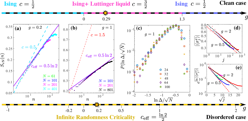
Figure 1: Overview of the interacting Majorana chain model Eq. (1). Top and bottom arrows present the phase diagrams for both clean and disordered models. The clean case (see Ref. Chepiga and Laflorencie ) displays three critical phases with central charges $c=1/2$ and $3/2$. Instead, the random case displays a unique Infinite Randomness Criticality, as demonstrated by representative cases in the various panels. (a-b) show the von-Neumann entanglement entropy $S_{\rm{vN}}(n)$ scaling as a function of subsystem length $n$, for $g=0.2$ and $g=1$ for which the clean scalings (with $c=0.5$ and $c=1.5$) are compared with the disorder-average EE for various lengths $N$, which exhibit the IRFP scaling with $c_{\rm eff}=0.5\,{\ln 2}$ (see also Fig. 2 below). Panel (c) presents another smoking gun of IRFP with the universal collapse for the distribution of the lowest gap $P\left(\frac{\ln\Delta}{\sqrt{N}}\right)$, displayed for $g=1$ and various system sizes $N$, see also Fig. 3. Panels (d-e) show the decay of the average and typical magnetizations, away form the boundary, for two representative cases $g=0.5$ and $g=2$ showing perfect agreement with IRFP criticality, see also Fig. 4 for more details and results. The yellow stars on top and bottom arrows denote the onset of incommensurability, further discussed in Fig. 5.

Such an unbounded entanglement growth Eq. (5) strongly contrasts with MBL or Anderson insulators for which a strict area law is observed, even at infinite temperature, with an EE bounded by the finite localization length Bauer and Nayak (2013); Laflorencie (2022). Here, the IRFP is only marginally localized, i.e., that all single-particle states have a finite localization length, except in the band center where the localization is stretched exponential Eggarter and Riedinger (1978); Fisher (1994); Nandkishore and Potter (2014).

III IRFP and interactions

Two historical examples of non-interacting IRFPs are the 1D disordered TFI model Fisher (1992, 1995), and the random-bond XX chain Fisher (1994). Interestingly, both models can be seen as the opposite sides of the same coin: non-interacting Majorana (real) vs. Dirac (complex) fermions with random hoppings. Although the effect of interactions was quickly understood as irrelevant in a Renormalization Group (RG) sense Doty and Fisher (1992); Fisher (1994) for free Dirac fermions, the story turned out to be quite different in the case of Majoranas. In his seminal work, Fisher first suggested that interactions should also be irrelevant at the IRFP in the Ising/Majorana case Fisher (1995), but this issue remained essentially unexplored for many years, before re-emerging only recently in the MBL context Pekker et al. (2014); Slagle et al. (2016); You et al. (2016); Monthus (2018); Sahay et al. (2021); Moudgalya et al. (2020); Laflorencie et al. (2022); Wahl et al. (2022). There at high energy, the IRFP was found to be destablized by weak interactions towards a delocalized ergodic phase Sahay et al. (2021); Moudgalya et al. (2020); Laflorencie et al. (2022).

Despite these progress made at high energy, the status of the ground-state of the disordered IMC model Eq. (1) is still controversial, with rather intriguing recent conclusions Milsted et al. (2015); Karcher et al. (2019) contrasting with previous claims Fisher (1995). Building on DMRG simulations Milsted et al. Milsted et al. (2015) observed a saturation of the EE for repulsive interaction $g>0$, in agreement with Karcher et al. Karcher et al. (2019) who further concluded that the system gets localized and spontaneously breaks the duality symmetry of the IMC Hamiltonian, for any $g>0$. Results in the attractive regime $g<0$, again based on EE scaling, are more ambiguous: Ref. Milsted et al. (2015) concludes that IRFP is stable, while Ref. Karcher et al. (2019) states on the contrary that disorder becomes irrelevant and that the clean fixed point physics is recovered.

IV Main results and phase diagram

Our work falls within this puzzling and stimulating context. By pushing the limits of DMRG simulations for disordered quantum systems note_dmrg , we carefully and deeply explore the ground-state properties of the IMC model Eq. (1) in the presence of both interactions and randomness. Our main result, summarized in Fig. 1, is that the IRFP is robust and stable to finite interactions. While in the clean case Rahmani et al. (2015b); Chepiga and Laflorencie , a succession of critical phases is observed upon varying $g$, with central charges $c=1/2,\,3/2$, adding disorder to the Majorana hopping terms is a relevant perturbation. For the range of interactions considered in this work, the non-interacting IRFP appears to be the unique attractive fixed point, thus reinforcing the original expectation Fisher (1995) that interactions are therefore irrelevant to the free Majorana IRFP.

Our conclusions are based on the complementarity of key observables used to probe the various aforementioned properties of the IRFP. This is exemplified in Fig. 1 where the von-Neumann EE (a-b), the low-energy gap (c), and the average and typical order parameters (d-e) are displayed across the various regimes of interaction strength, all panels showing one of the smoking gun feature characteristic of the IRFP.

In the rest of the work, we present and discuss very carefully our numerical results building on these three pivotal observables, several technical aspects being detailed in the supplementary material sm . Let us however mention that we simulate the IMC model Eq. (1) in its "magnetic" version Eq. (2), and mostly focus on the repulsive $g>0$ regime. Although interesting effects are certainly expected away from it, we stick to the self-dual line ${\overline{\ln J}}={\overline{\ln h}}$, independently drawing $J_{i}$ and $h_{i}$ from a box $[1-W,1+W]$ with $W=0.9$ noteW . A very important issue, sometimes overlooked, concerns the number of random samples which we take as large as possible (typically between $3000$ and $8000$). This is particularly meaningful at IRFPs where rare events play a pivotal role, and broad distributions are crucially important to describe the physics.

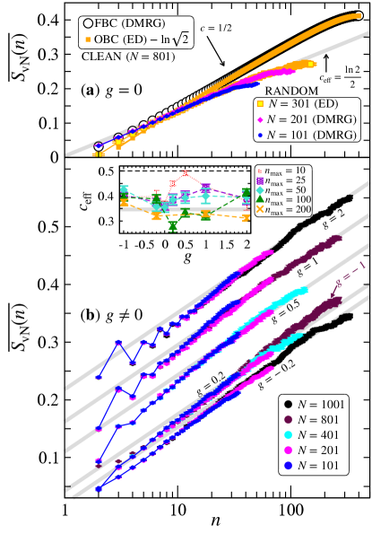
Figure 2: DMRG and ED results for the von-Neumann entropy scaling as a function of sub-system size $n$ for (a) non-interacting, and (b) interacting Majorana fermions, Eq. (1). (a) $g=0$, clean chain results (upper data) illustrate how OBC ED data match with FBC DMRG (after subtracting the boundary entropy $\ln\sqrt{2}$). In the random case, a similar agreement is observed for the disorder-average (after the same subtraction), the dominant scaling being now controlled by Eq. (5) with an "effective central charge" $c_{\rm eff}=\frac{\ln 2}{2}$ (grey line), a finite-size bending down is observed when half-chain is approached. (b) $g\neq 0$ DMRG results shown for subsystems $2\leq n\leq N/3$, various interaction strengths (indicated on the plot), and different chain lengths (colored symbols). The agreement with the IFRP scaling (grey line Eq. (5) with $c_{\rm eff}=\frac{\ln 2}{2}$) is excellent in all cases, once the asymptotic regime is reached beyond a finite crossover length scale Laflorencie et al. (2004); Laflorencie (2022). Inset: $g$-dependence of $c_{\rm eff}$ extracted from fits to the form Eq. (5) over successive sliding windows ending at $n_{\rm max}$. All data agree with the asymptotic log scaling controlled by the prefactor $c_{\rm eff}=\frac{\ln 2}{2}$.

V Entanglement entropy

Before getting to the EE itself, we start with a brief discussion of the boundary conditions, illustrated for the non-interacting case in Fig. 2 (a). Instead of open boundary conditions (OBC), most commonly used in the DMRG realm, here we shall use the so-called fixed boundary conditions (FBC), obtained by locally pinning the boundary spins with a strong longitudinal field Zhou et al. (2006); Affleck et al. (2009), thus artificially breaking the parity symmetry of the IMC Hamiltonian. As a result, the FBC entropy is reduced from its OBC value by the Affleck-Ludwig boundary term Affleck and Ludwig (1991), such that $S_{\rm vN}^{\rm FBC}=S_{\rm vN}^{\rm OBC}-\ln\sqrt{2}$, but does not loose its universal logarithmic scaling. This becomes clear in Fig. 2 (a) for free fermions ($g=0$) where DMRG and exact diagonalization (ED) data are successfully compared in the clean case. Interestingly, we further observe that such a boundary entropy also shows up for the free-fermion IRFP, as evidenced in the same panel (a) of Fig. 2 where OBC ED data match with FBC DMRG after a subtraction of the similar $\ln\sqrt{2}$ term.

Let us now present the most important result of the paper, displayed in Fig. 2 (b) where for finite interaction strengths $g\neq 0$, the disorder-average EEs show excellent agreement with the non-interacting IFRP logarithmic growth Eq. (5), with $c_{\rm eff}=\frac{\ln 2}{2}$. Remarkably, this remains true for the entire regime of study $-1\leq g\leq 2$. This is even more clear from the inset where the $g$-dependence of $c_{\rm eff}$ is extracted from fits to the form Eq. (5) over successive sliding windows. This result deeply contrasts with previous works Milsted et al. (2015); Karcher et al. (2019) where a saturation of EE was observed and interpreted as a consequence of localization. There are two main causes for this disagreement, both due to numerical limitations that most probably led to a misinterpretation of earlier DMRG data. The first reason is the number of kept DMRG states, which can be a major obstacle note_dmrg . The second, perhaps more interesting, comes from the boundary conditions and our choice of FBC, which leads to a significant reduction in EE, giving a decisive advantage to our DMRG simulations sm .

It is furthermore noteworthy that all finite interaction results show the same tendency to flow to the non-interacting IRFP scaling, with a unique effective central charge fully compatible with $c_{\rm eff}=\frac{\ln 2}{2}$, even in the repulsive regime where the clean case displays $c=3/2$ for $0.29\leq g\leq 1.3$, as clearly visible in Fig. 1 (b) for a comparison between clean and disordered cases at $g=1$.

VI Low-energy gap

In order to double-check the IRFP hypothesis over the broad regime of interaction strengths, we also focus on the lowest energy gap $\Delta$ above the ground-state, and in particular we aim to check the very peculiar exponentially activated scaling law defined by Eq. (3), which signals a dynamical exponent $z=\infty$. In addition, the probability distribution of these gaps is expected to display broadening and a universal scaling form, as shown for free fermions Young and Rieger (1996); Fisher and Young (1998).

Here for the interacting model, we also observe, see Fig. 3 (a) for $g=0.5$, a very clear broadening of the distributions $P(\ln\Delta)$ upon increasing the system size, which is a strong evidence that $z=\infty$, as predicted for the IRFP. Furthermore, the same data show an excellent collapse in Fig. 3 (b) when histogrammized against $({\ln\Delta})/{\sqrt{N}}$, without any adjustable parameter. We have checked that this remains true for other values of the interaction strength (in the range of study), as shown for a few values of $g$ in the inset of Fig. 3 (b). There, one sees that the typical gap $e^{\overline{\ln\Delta}}$ perfectly obeys the activated scaling law Eq. (3). The non-interacting case (ED data for $g=0$) is also displayed for comparison.

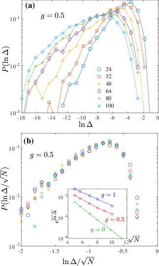
Figure 3: DMRG results for the lowest energy gap $\Delta$. (a) Distribution $P(\ln\Delta)$ collected at $g=0.5$ from $4000$ samples for various system sizes, as indicated on the plot. The broadening upon increasing $N$ is an IRFP signature, best seen in (b) where the distributions of rescaled gaps $P\left({\ln\Delta}/{\sqrt{N}}\right)$ show very good collapse. Inset: the typical gap plotted vs. $\sqrt{N}$ for $g=0,\,0.5,\,1$, shows perfect agreement with the activated IRFP scaling Eq. (3).

VII Correlations

The last evidence for infinite randomness physics is captured by the spin correlations, as given by Eq. (4). The absence of self-averaging is again reflected here in the clear qualitative difference between mean and typical decays of pairwise correlations: power-law with a universal exponent $\eta={\frac{3-\sqrt{5}}{2}}\approx 0.382$ vs. stretched exponential. This IRFP feature can also be nicely captured with FBC. Indeed, when the edge spins are fixed, the following decrease of the order parameter is expected away from the boundary

$${\overline{|\langle\sigma_{j}^{x}\rangle|}}\sim{j^{-\eta/2}}\quad{\rm{and}}\quad{\overline{\ln\,|\langle\sigma_{j}^{x}\rangle|}}\sim-\sqrt{j}.$$ (6)

This behavior is readily observed in Fig. 4 where panels (a) and (b) show a comparison between average and typical decays for a few representative values of the interaction strength. The extracted exponent governing the average is fully consistent with the universal IRFP value $\eta=2-\phi$ Fisher (1992), where $\phi$ is the golden mean. The typical decay, while suffering from finite size effects, also appears to be in good agreement with a stretched exponential vanishing.

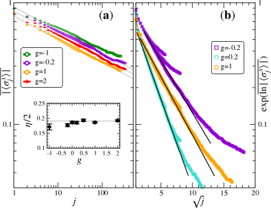
Figure 4: DMRG results for the decrease of the order parameter away from the boundary $j$, see Eq. (6). (a) Power-law decay of the disorder-average ${\overline{|\langle\sigma_{j}^{x}\rangle|}}$ shown for 4 different values of the interaction $g$, all in excellent agreement with the IRFP prediction $\eta/2=1-\phi/2\approx 0.191$ (grey line). Inset: estimated exponent $\eta/2$ plotted against $g$. (b) The stretched exponential vanishing of the typical value $\exp({{\overline{\ln\,|\langle\sigma_{j}^{x}\rangle|}}})$ is fully compatible with the IRFP scaling (black lines).

VIII Incommensurability

So far we have focused on the absolute value of the magnetization, ignoring possible commensurate or incommensurate (IC) modulations. However, while the mean of the absolute value ${\overline{|\langle\sigma_{j}^{x}\rangle|}}$ does decay algebraically, the mean magnetization vanishes much faster ${\overline{\langle\sigma_{j}^{x}\rangle}}\propto\exp\left(-j/\xi\right)\cos(qj)$, with antiferromagnetic correlations ($q=\pi$) for $g\leq g^{\star}$, which then turns IC ($\pi/2<q<\pi$) beyond $g^{\star}\approx 0.18$, see Fig. 5. It is noteworthy that the IC behavior induced by the frustrating nature of the interaction is not pinned by the disorder, as previously suggested Milsted et al. (2015), but actually seems to be enhanced compared to the clean case for which $g^{\star}_{\rm clean}\approx 0.29$ Chepiga and Laflorencie . Nevertheless, IC is only short-range because the Luttinger liquid is localized by the disorder.

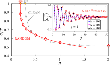
Figure 5: IC wave-vector $q$ extracted from exponential scaling of average magnetization away from the polarized boundary ($g^{\star}\approx 0.18$, red symbols), compared to the clean case Chepiga and Laflorencie ($g^{\star}_{\rm clean}\approx 0.29$, grey symbols). Inset: Average magnetization decay away from the boundary shown at $g=1$ for various lengths $N$ and compared to the fit.

IX Discussions and conclusions

In the strong-disorder RG (SDRG) framework Fisher (1992, 1995); Igloi and Monthus (2005), adding (moderate) interactions to the random-bond XX chain only brings negligible modifications to the RG recursion relations, and the IRFP has the very same form as in the non-interacting XX case, notably for the Heisenberg chain Fisher (1994). However, this is less obvious for the interacting version of the TFIM, as recently discussed by Monthus Monthus (2018) who showed that the SDRG treatment of disordered interacting Majorana fermions generates higher-order couplings, which prevents direct conclusions about the effects of interactions, a situation also encountered for more general random XYZ models Roberts and Motrunich (2021) as well as for MBL Pekker et al. (2014); Slagle et al. (2016); You et al. (2016).

In such a puzzling context, our numerical work substantially clarifies the problem, providing a simple picture which contrast with previous works Milsted et al. (2015); Karcher et al. (2019). Building on state-of-the-art DMRG simulations, appropriate boundary conditions, and a very large number of samples, we demonstrate that the non-interacting IRFP is stable against attractive and repulsive interactions between Majorana fermions. This solves a relatively old problem, and open interesting questions regarding the stability of the marginally localized Nandkishore and Potter (2014) IRFP far from the ground-state where instead, weak interactions are expected to delocalize and restore ergodicity, at least in the infinite-temperature limit Sahay et al. (2021); Moudgalya et al. (2020); Laflorencie et al. (2022), thus suggesting a possible critical point at finite energy density above the ground-state.

X Acknowledgments

We thank J. Hoyos and I. C. Fulga for comments. NC acknowledges LPT Toulouse (CNRS) for hospitality. This work has been supported by Delft Technology Fellowship, by the EUR grant NanoX No. ANR-17-EURE-0009 in the framework of the ”Programme des Investissements d’Avenir”. Numerical simulations have been performed at the DelftBlue High Performance Computing Centre (tudelft.nl/dhpc) and CALMIP (grants 2022-P0677).

Supplemental material

XI Models and useful transformations

The interacting Majorana chain model studied in the main text is governed by the one-dimensional Hamiltonian

$${\cal{H}}=-\sum_{j}\left({\rm{i}}t_{j}\gamma_{j}\gamma_{j+1}+g\gamma_{j}\gamma_{j+1}\gamma_{j+2}\gamma_{j+3}\right),$$ (S1)

with random couplings $t_{j}$ and constant interaction $g$. It is more convenient to introduce odd and even Majorana operators $\gamma_{2j-1}=a_{\ell}\quad{\rm{and}}\quad\gamma_{2j}=b_{\ell}$, These new operators are connected to the real space lattice sites $\ell$ where live Dirac fermions and Pauli matrices operators. We use the Jordan-Wigner mapping

$$a_{\ell} = c_{\ell}^{\dagger}+c_{\ell}^{\vphantom{\dagger}}=K_{\ell}\sigma^{x}_{\ell}$$ (S2)

$$b_{\ell} = {\rm{i}}(c_{\ell}^{\dagger}-c_{\ell}^{\vphantom{\dagger}})=K_{\ell}\sigma^{y}_{\ell}$$ (S3)

$$a_{\ell}b_{\ell} = {\rm{i}}(1-2c_{\ell}^{\dagger}c_{\ell}^{\vphantom{\dagger}})={\rm{i}}\sigma_{\ell}^{z}$$ (S4)

$${\rm{with}}\quad K_{\ell} = \prod_{k=1}^{\ell-1}\sigma_{k}^{z},$$ (S5)

such that the above interacting Majorana chain can be expressed in three languages: Pauli, Majorana, and Dirac, as sketched in Fig. S1. It is also instructive to inroduce the possibility for asymmetric interactions $g_{x,z}$, such that Eq. (S1) reads

$${\cal{H}}_{\rm Majorana} = -{\rm{i}}\sum_{\ell}\left(J_{\ell}b_{\ell}a_{\ell+1}-h_{\ell}a_{\ell}b_{\ell}\right)$$

$$- \sum_{\ell}\left(g_{z}a_{\ell}b_{\ell}a_{\ell+1}b_{\ell+1}+g_{x}b_{\ell}a_{\ell+1}b_{\ell+1}a_{\ell+2}\right),$$

with $J_{\ell}=t_{2j}$ and $h_{\ell}=t_{2j-1}$, as sketched in Fig. S1 (b). In the Pauli (spin) language, the same model becomes

$${\cal{H}}_{\rm Pauli} = \sum_{\ell}\left(J_{\ell}\sigma^{x}_{\ell}\sigma^{x}_{\ell+1}-h_{\ell}\sigma^{z}_{\ell}\right)$$ (S7)

$$+ \sum_{\ell}\left(g_{z}\sigma^{z}_{\ell}\sigma^{z}_{\ell+1}+g_{x}\sigma^{x}_{\ell}\sigma^{x}_{\ell+2}\right)$$

where $\sigma^{x,z}_{\ell}$ are Pauli matrices at site $\ell$, see Fig. S1 (a). Finally, in terms of Dirac fermions, we have the interacting version of the Kitaev chain model Kitaev (2001), illustrated in Fig. S1 (c)

$${\cal{H}}_{\rm Dirac} = \sum_{\ell}\Bigl{[}J_{\ell}\left(c_{\ell}^{\dagger}c_{\ell+1}^{\vphantom{\dagger}}+c_{\ell}^{\dagger}c_{\ell+1}^{{\dagger}}+{\rm{h.c.}}\right)+2h_{\ell}n_{\ell}\Bigr{]}$$

$$+ g_{z}\sum_{\ell}\left(1-2n_{\ell}\right)\left(1-2n_{\ell+1}\right)$$

$$+ g_{x}\sum_{\ell}\left(c_{\ell}^{\dagger}-c_{\ell}^{\vphantom{\dagger}}\right)\left(1-2n_{\ell+1}\right)\left(c_{\ell+2}^{\dagger}+c_{\ell+2}^{\vphantom{\dagger}}\right).$$

The $g_{z}$ coupling is a simple density-density interaction term at distance 1: $\sim g_{z}n_{\ell}n_{\ell+1}$. Instead, the $g_{x}$ coupling brings frustration to the problem and displays the very interesting density-assisted hopping $\sim g_{x}c_{\ell}^{\vphantom{\dagger}}n_{\ell+1}c_{\ell+2}^{\dagger}$ and pairing $\sim g_{x}c_{\ell}^{{\dagger}}n_{\ell+1}c_{\ell+2}^{\dagger}$ terms at distance 2.

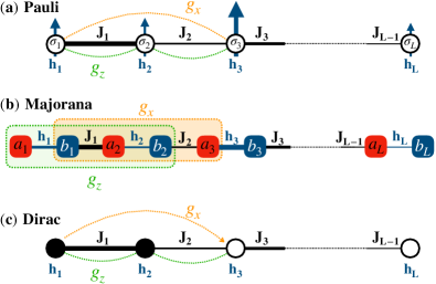
Figure S1: Schematic picture for the same interacting Majorana chain model. (a) Spin Hamiltonian Eq. (S7), (b) Majorana fermion representation Eq. (XI), (c) Dirac fermions Eq. (XI).

XII Entanglement entropy distribution

Here we show several examples of middle-chain entanglement entropy distributions in Fig. S2 for various interaction strengths and system sizes. Upon increasing $N$, one sees a slow crossover towards IRFP physics signalled by a peak at $S_{\rm vN}\approx\ln 2$ Refael and Moore (2004); Laflorencie (2005). Interestingly, for $g=-0.2$ and $g=0.2$ there is also a peak at zero entropy, but it slowly decreases with growing $N$ while its weight is transferred to $\ln 2$. This is not observed for $g=1,\,2$ due to this large coupling strength, which prevents zero entanglement (see e.g. Fig. S1 (a) with $g_{x}=g_{z}$).

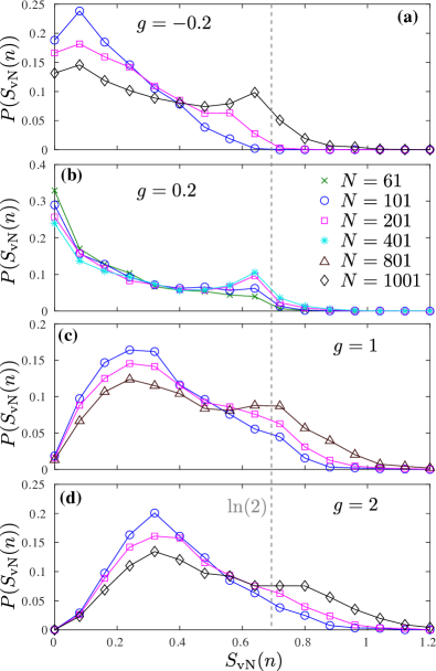
Figure S2: Entanglement entropy distribution for four different coupling contants $g$ and various system sizes. The probability develops a peak at $\ln(2)$ typical for infinite randomness critical point. The peak at zero for weak interaction is gradually depleted with increasing $N$ (a-b), while it is already quasi-absent at large $g$ (c-d) because the disorder-free interaction terms prevent to have cut with $S_{\rm vN}=0$.

XIII Additional results on incommensurate correlations

In Fig.S3 we provide additional numerical results for incommensurate Friedel oscillations that appear as a response to a boundary spin polarized in $x$-direction. We show results for five different values of the coupling constant ranging from $g=0.2$ that in the clean case is located below the Lifshitz point (i.e. in the region where the correlations are still commensurate) to the strongly-interacting case $g=2$, where the extracted wave-vector $q\approx 0.515\pi$ fully agrees (the difference is less than $1\%$) with the value of $q$ in the clean case.

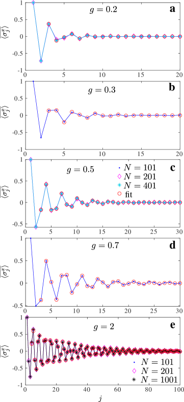
Figure S3: Disorder-average magnetization in the vicinity of the polarized edge spin for $N=101$ (blue), $N=201$ (magenta), $N=401$ (cyan) and $N=1001$ (black) for various values of the coupling contant $g$. Red open circles are fit with $\propto e^{-j/\xi}\cos(q\cdot j+\phi_{0})$. The extracted values of $q$ are summarized in Fig. 5 of the main text.

XIV Extracting energy gaps with DMRG

In order to extract the energy gap, we target several low-lying eigenstates of the effective Hamiltonian at every DMRG iteration and keep track of the energy as a function of iteration. Following Ref. Chepiga and Mila (2017) we associate reliable energy levels with energies that remains flat for several DMRG iterations. In practice, the flat intervals span over almost the entire chain length except very close to the edges, where the effective basis is known to be too small to properly capture an excited state. Such an excellent convergence of the excitation energy for disordered systems is quite surprising but systematically good from sample to sample. Probably the reason behind it is an infinite correlation length, for this the used method is known to be extremely accurateChepiga and Mila (2017); Chepiga (2022). The approach is troublesome for very small gaps (of the order of $10^{-8}$ and below), however considered values of $g$ this has a noticeable contribution on a disordered chains with length above $80-100$ sites.

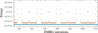
Figure S4: Example of a DMRG convergence of the two lowest energy levels for a selected sample with $N=80$, $g=0.5$ as a function of DMRG iterations. Regions where the first excitation energy (red dots) is flat as a function of DMRG iterations corresponds to a reliable value of the excitation energy. Periodic increase of the energy of the first excited state takes place close to the edges of the chain and is a typical artifact of the method. In the presented case the energy gap is $\Delta\approx 2\cdot 10^{-5}$.

References

- Alet and Laflorencie (2018) F. Alet and N. Laflorencie, C. R. Phys. 19, 498 (2018).
- Abanin et al. (2019) D. A. Abanin, E. Altman, I. Bloch, and M. Serbyn, Rev. Mod. Phys. 91, 021001 (2019).
- Fleishman and Anderson (1980) L. Fleishman and P. W. Anderson, Phys. Rev. B 21, 2366 (1980).
- Gornyi et al. (2005) I. V. Gornyi, A. D. Mirlin, and D. G. Polyakov, Phys. Rev. Lett. 95, 206603 (2005).
- Basko et al. (2006) D. M. Basko, I. L. Aleiner, and B. L. Altshuler, Annals of Physics 321, 1126 (2006).
- Sierant et al. (2020) P. Sierant, D. Delande, and J. Zakrzewski, Phys. Rev. Lett. 124, 186601 (2020).
- Abanin et al. (2021) D. A. Abanin, J. H. Bardarson, G. De Tomasi, S. Gopalakrishnan, V. Khemani, S. A. Parameswaran, F. Pollmann, A. C. Potter, M. Serbyn, and R. Vasseur, Annals of Physics 427, 168415 (2021).
- Brighi et al. (2022) P. Brighi, A. A. Michailidis, D. A. Abanin, and M. Serbyn, Phys. Rev. B 105, L220203 (2022).
- Sierant and Zakrzewski (2022) P. Sierant and J. Zakrzewski, Phys. Rev. B 105, 224203 (2022).
- Sels (2022) D. Sels, Phys. Rev. B 106, L020202 (2022).
- Morningstar et al. (2022) A. Morningstar, L. Colmenarez, V. Khemani, D. J. Luitz, and D. A. Huse, Phys. Rev. B 105, 174205 (2022).
- Rahmani et al. (2015a) A. Rahmani, X. Zhu, M. Franz, and I. Affleck, Phys. Rev. Lett. 115, 166401 (2015a).
- Rahmani et al. (2015b) A. Rahmani, X. Zhu, M. Franz, and I. Affleck, Phys. Rev. B 92, 235123 (2015b).
- Milsted et al. (2015) A. Milsted, L. Seabra, I. C. Fulga, C. W. J. Beenakker, and E. Cobanera, Phys. Rev. B 92, 085139 (2015).
- Karcher et al. (2019) J. F. Karcher, M. Sonner, and A. Mirlin, Phys. Rev. B 100, 134207 (2019).
- (16) N. Chepiga and N. Laflorencie, arXiv:2211.15598 (SciPost Phys. 2023, in press).
- Kitaev (2001) A. Y. Kitaev, Phys.-Usp. 44, 131 (2001).
- (18) See the supplemental material for details and additional results.
- Pfeuty (1970) P. Pfeuty, Annals of Physics 57, 79 (1970).
- Fisher (1992) D. S. Fisher, Phys. Rev. Lett. 69, 534 (1992).
- Fisher (1995) D. S. Fisher, Phys. Rev. B 51, 6411 (1995).
- Igloi and Monthus (2005) F. Igloi and C. Monthus, Phys. Rep. 412, 277 (2005).
- Young and Rieger (1996) A. P. Young and H. Rieger, Phys. Rev. B 53, 8486 (1996).
- Henelius and Girvin (1998) P. Henelius and S. M. Girvin, Phys. Rev. B 57, 11457 (1998).
- Huang and Moore (2014) Y. Huang and J. E. Moore, Phys. Rev. B 90, 220202 (2014).
- Laflorencie (2022) N. Laflorencie, in Quantum Science and Technology (Springer International Publishing, 2022) pp. 61–87.
- Holzhey et al. (1994) C. Holzhey, F. Larsen, and F. Wilczek, Nucl. Phys. B 424, 443 (1994).
- Vidal et al. (2003) G. Vidal, J. I. Latorre, E. Rico, and A. Kitaev, Phys. Rev. Lett. 90, 227902 (2003).
- Calabrese and Cardy (2004) P. Calabrese and J. Cardy, J. Stat. Mech. 06, P06002 (2004).
- Refael and Moore (2004) G. Refael and J. E. Moore, Phys. Rev. Lett. 93, 260602 (2004).
- Refael and Moore (2009) G. Refael and J. E. Moore, J. Phys. A 42, 504010 (2009).
- Laflorencie (2005) N. Laflorencie, Phys. Rev. B 72, 140408 (2005).
- Hoyos et al. (2007) J. A. Hoyos, A. P. Vieira, N. Laflorencie, and E. Miranda, Phys. Rev. B 76, 174425 (2007).
- Fagotti et al. (2011) M. Fagotti, P. Calabrese, and J. E. Moore, Phys. Rev. B 83, 045110 (2011).
- Bauer and Nayak (2013) B. Bauer and C. Nayak, J. Stat. Mech. 2013, P09005 (2013).
- Eggarter and Riedinger (1978) T. P. Eggarter and R. Riedinger, Phys. Rev. B 18, 569 (1978).
- Fisher (1994) D. S. Fisher, Phys. Rev. B 50, 3799 (1994).
- Nandkishore and Potter (2014) R. Nandkishore and A. Potter, Phys. Rev. B 90, 195115 (2014).
- Doty and Fisher (1992) C. A. Doty and D. S. Fisher, Phys. Rev. B 45, 2167 (1992).
- Pekker et al. (2014) D. Pekker, G. Refael, E. Altman, E. Demler, and V. Oganesyan, Phys. Rev. X 4, 011052 (2014).
- Slagle et al. (2016) K. Slagle, Y.-Z. You, and C. Xu, Phys. Rev. B 94, 014205 (2016).
- You et al. (2016) Y.-Z. You, X.-L. Qi, and C. Xu, Phys. Rev. B 93, 104205 (2016).
- Monthus (2018) C. Monthus, J. Phys. A: Math. Theor. 51, 115304 (2018).
- Sahay et al. (2021) R. Sahay, F. Machado, B. Ye, C. R. Laumann, and N. Y. Yao, Phys. Rev. Lett. 126, 100604 (2021).
- Moudgalya et al. (2020) S. Moudgalya, D. A. Huse, and V. Khemani, arXiv:2008.09113 (2020).
- Laflorencie et al. (2022) N. Laflorencie, G. Lemarié, and N. Macé, Phys. Rev. Research 4, L032016 (2022).
- Wahl et al. (2022) T. B. Wahl, F. Venn, and B. Béri, Phys. Rev. B 105, 144205 (2022).
- (48) In our DMRG simulations we keep up to states, perform from 4 to 8 sweeps and discard singular values lower than . In order to avoid convergence to a stable local minima at the low interactions () we target multiple states in the Lanczos subroutine that prevents the system from being stacked at the low-lying excited state.
- (49) We explicitly chose close to but in order to avoid numerical limitations of the DMRG when . It is interesting to note that Refs. Milsted et al. (2015); Karcher et al. (2019) also took box disorder, but with a weaker randomness , which may increase crossover effects Laflorencie et al. (2004) that hinder the establishment of the asymptotic IRFP regime.
- Laflorencie et al. (2004) N. Laflorencie, H. Rieger, A. W. Sandvik, and P. Henelius, Phys. Rev. B 70, 054430 (2004).
- Zhou et al. (2006) H.-Q. Zhou, T. Barthel, J. O. Fj\a erestad, and U. Schollwöck, Phys. Rev. A 74, 050305 (2006).
- Affleck et al. (2009) I. Affleck, N. Laflorencie, and E. S. Sørensen, J. Phys. A 42, 504009 (2009).
- Affleck and Ludwig (1991) I. Affleck and A. W. W. Ludwig, Phys. Rev. Lett. 67, 161 (1991).
- Fisher and Young (1998) D. S. Fisher and A. P. Young, Phys. Rev. B 58, 9131 (1998).
- Roberts and Motrunich (2021) B. Roberts and O. I. Motrunich, Phys. Rev. B 104, 214208 (2021).
- Chepiga and Mila (2017) N. Chepiga and F. Mila, Phys. Rev. B 96, 054425 (2017).
- Chepiga (2022) N. Chepiga, SciPost Phys. Core 5, 031 (2022).